Local-time representation of path integrals

Abstract

Abstract

We derive a local-time path-integral representation for a generic one-dimensional time-independent system. In particular, we show how to rephrase the matrix elements of the Bloch density matrix as a path integral over $x$-dependent local-time profiles. The latter quantify the time that the sample paths $x(t)$ in the Feynman path integral spend in the vicinity of an arbitrary point $x$. Generalization of the local-time representation that includes arbitrary functionals of the local time is also provided. We argue that the results obtained represent a powerful alternative to the traditional Feynman–Kac formula, particularly in the high and low temperature regimes. To illustrate this point, we apply our local-time representation to analyze the asymptotic behavior of the Bloch density matrix at low temperatures. Further salient issues, such as connections with the Sturm–Liouville theory and the Rayleigh–Ritz variational principle are also discussed.

I Introduction

The path integral (PI) has been used in quantum physics since the revolutionary work of Feynman Feynman1948 , although the basic observation goes back to Dirac Dirac33 ; Dirac35 who appreciated the rôle of the Lagrangian in short-time evolution of the wave function, and even suggested the time-slicing procedure for finite, i.e., non-infinitesimal, time lags. Since then the PI approach yielded invaluable insights into the structure of quantum theory FeynmanHibbs and provided a viable alternative to the traditional operator-formalism-based canonical quantization. During the second half of the 20th century, the PI became a standard tool in quantum field theory Ramond and statistical physics Zinn , often providing the easiest route to derivation of perturbative expansions and serving as an excellent framework for (both numerical and analytical) non-perturbative analysis Kleinert .

Feynman PI has its counterpart in pure mathematics, namely, in the theory of continuous-time stochastic processes RevuzYor . There the concept of integration over a space of continuous functions (so-called fluctuating paths or sample paths) had been introduced by Wiener Wiener1923 already in 1920’s in order to represent and quantify the Brownian motion. Interestingly enough, this so-called Wiener integral (or integral with respect to Wiener measure) was formulated 2 years before the discovery of the Schrödinger equation and 25 years before Feynman’s PI formulation.

The local time for a Brownian particle (in some literature also called sojourn time) has been of interest to physicists and mathematicians, since the seminal work of Paul Lévy in 1930’s Levy1939 . In its essence, the local time characterizes the time that a sample trajectory $x(t)$ of a given stochastic process spends in the vicinity of an arbitrary point $X$. This in turn defines a sample trajectory $L^{X}$ of a new stochastic process. A rich theory has been developed for local-time processes that stem from diffusion processes (see, e.g., Ref. Marcus and citations therein). For later convenience, we should particularly highlight the Ray–Knight theorem which states that the local time of the Wiener process can be expressed in terms of the squared Bessel process Borodin ; Ray ; Knight . In contrast to mathematics, the concept of the local time is not uniquely settled in physics literature. Various authors define essentially the same quantity under different names (local time, occupation time, traversal time, etc.), and with different applications in mind. For example, in Ref. Sokolovski the traversal time is used to study quantum scattering and tunneling processes, in Paulin the small-temperature behavior of the equilibrium density matrix is analyzed with a help of the occupation time, while in Ref. Luttinger1982 the large-time behavior of path integrals that contain functionals of the local time is discussed.

The aim of this paper is to derive a local-time PI representation of the Bloch density matrix, i.e., the matrix elements $\left\langle x_{b}\right|e^{-\beta\hat{H}}\left|x_{a}\right\rangle$ of the Gibbs operator. This can serve not only as a viable alternative to the commonly used Feynman–Kac representation but also as a powerful tool for extracting both large and small-temperature behavior. Apart from the general theoretical outline, our primary focus here will be on the low-temperature behavior which is technically more challenging than the large-temperature regime. In fact, the large-temperature expansion was already treated in some detail in our previous paper JizbaZatl . Last but not least, we also wish to promote the concept of the local time which is not yet sufficiently well known among the path-integral practitioners.

The structure of the paper is as follows. To set the stage we recall in the next section some fundamentals from the Feynman PI which will be needed in later sections. In Section III we provide motivation for the introduction of a local time, and construct a heuristic version of the local-time representation of PI’s. The key technical part of the article is contained in Section IV, where we derive by means of the replica trick the local-time representation of the Bloch density matrix. Relation to the Sturm–Liouville theory is also highlighted in this context. A local-time analog of the Feynman–Matthews–Salam formula LvW ; BJV is presented in Section V and its usage is illustrated with a computation of the one-point distribution of the local time. Since a natural arena for local-time PI’s is in thermally extremal regimes, we confine our attention in Section VI on large- and small-$\beta$ asymptotic behavior of the Bloch density matrix. There we also derive an explicit leading-order behavior in large-$\beta$ (i.e., low-temperature) expansion. The analysis is substantially streamlined by using the Rayleigh–Ritz variational principle. Finally, Section VII summarizes our results and discusses possible extensions, applications, and future developments of the present work. For the reader’s convenience the paper is supplemented with appendix which clarifies some finer technical details.

II Path-integral representation of the Bloch density matrix

Consider a non-relativistic one-dimensional quantum-mechanical system described by a time-independent Hamiltonian $\hat{H}=\frac{\hat{p}^{2}}{2M}+V(\hat{x})$ where $\hat{p}\left|x\right\rangle=-i\hbar\partial_{x}\left|x\right\rangle$. Throughout this paper we will study the matrix elements

$$\rho(x_{a},x_{b},\beta)\ \equiv\ \left\langle x_{b}\right|e^{-\beta\hat{H}}\left|x_{a}\right\rangle\,,$$ (1)

of the Gibbs operator $e^{-\beta\hat{H}}$, where $\beta=1/(k_{B}T)$ is the inverse temperature and $k_{B}$ is the Boltzmann constant. The matrix $\rho(x_{a},x_{b},\beta)$, known also as the Bloch density matrix, is a fundamental object in quantum statistical physics, as the expectation value of an operator $\hat{O}$ at the temperature $T$ can be written in the form

$$\langle\hat{O}\rangle\ =\ \frac{1}{Z}\int_{\mathbb{R}}\int_{\mathbb{R}}dx_{a}dx_{b}\ \!\ \!\rho(x_{a},x_{b},\beta)\ \!\langle x_{b}|\hat{O}|x_{a}\rangle\,,$$ (2)

where $Z=\int_{\mathbb{R}}dx\ \!\rho(x,x,\beta)$ is the partition function of the system. In case of need, ensuing quantum mechanical transition amplitudes can be obtained from (1) via a Wick rotation which formally amounts to the substitution $\beta\rightarrow it/\hbar$, converting thus the Gibbs operator $e^{-\beta\hat{H}}$ to the quantum evolution operator $e^{-it\hat{H}/\hbar}$.

The matrix elements in Eq.(1) can be represented via the path integral as FeynmanHibbs ; Kleinert

$$\rho(x_{a},x_{b},\beta)\ =\ \int_{x(0)=x_{a}}^{x(\beta\hbar)=x_{b}}\!\!\!\mathcal{D}x(\tau)\exp\left\{-\frac{1}{\hbar}\int_{0}^{\beta\hbar}\!\!\!d\tau\left[\frac{M}{2}\dot{x}^{2}+V(x)\right]\right\}\,.$$ (3)

This represents a “sum” over all continuous trajectories $x(\tau)$, $\tau\in[0,\beta\hbar]$, connecting the initial point $x(0)=x_{a}$ with the final point $x(\beta\hbar)=x_{b}$. It should be noted that the integral $\int_{0}^{\beta\hbar}\!\!\!d\tau\left[\frac{M}{2}\dot{x}^{2}+V(x)\right]$ is the classical Euclidean action integral along the path $x(\tau)$ with $0<\tau\leq\beta\hbar$. In the following we will denote the Euclidean action as $\mathcal{A}$. The integrand in $\mathcal{A}$, i.e., $(M/2)\dot{x}^{2}(\tau)+V(x(\tau))$, can be identified with the classical Hamiltonian function, in which the momentum $p$ is substituted for $M\dot{x}$. One can also regard (3) as an expectation value of the functional $\exp[-\int_{0}^{\beta\hbar}\!d\tau\ \!V(x(\tau))/\hbar]$ over the (driftless) Brownian motion with the diffusion coefficient $M/2\hbar$, and duration $\beta\hbar$, that starts at point $x_{a}$, and terminates at $x_{b}$. The latter stochastic process is also known as Brownian bridge.

III Local-time representation of path integrals: heuristic approach

The purpose of this section is twofold. Firstly, we would like to motivate a need for reformulation of PI’s in the language of local-time stochastic process. In particular, we point out when such a reformulation can be more pertinent than the conventional “sum over histories” prescription. Secondly, we wish to outline a heuristic construction of the local-time representation of PI’s. More rigorous and explicit (but less intuitive) formulation of PI’s over ensemble of local times will be presented in the subsequent Section.

To provide a physically sound motivation for the local-time representation of PI’s we follow exposition of Paulin et al. in Ref. Paulin . To this end we first consider the diagonal elements of the Bloch density matrix, i.e., $\rho(x_{a},x_{a},\beta)$ (often referred to as the Boltzmann density). Upon shifting $x\rightarrow x+x_{a}$, and setting $x=\lambda\xi$, $\tau=s\beta\hbar$ ($\lambda\equiv\sqrt{\beta\hbar^{2}/M}$ is the thermal de Broglie wavelength), the PI (3) can be reformulated in terms of dimensionless quantities $s$ and $\xi(s)$ as

$$\rho(x_{a},x_{a},\beta)\ =\ \frac{1}{\lambda}\int_{x(0)=0}^{x(1)=0}\!\!\mathcal{D}\xi(s)\ \!\exp\left\{-\int_{0}^{1}\!\!\!ds\left[\frac{1}{2}\dot{\xi}^{2}+\beta V(x_{a}+\lambda\xi)\right]\right\}.$$ (4)

Note in particular, that in contrast to $\mathcal{D}x(\tau)$ the measure $\mathcal{D}\xi(s)$ does not explicitly depend on $\beta$, and thus $\beta$-dependent parts in the PI are under better control. Such a rescaled representation is particularly useful when discussing large- and/or small-$\beta$ behavior of the path integral in question. Path fluctuations in the potential are controlled by $\lambda\propto\sqrt{\beta}$, and the factor $\beta$ quantifies the significance of the potential $V$ with respect to the kinetic term.

For small $\beta$ (i.e., high temperature), typical paths $x(s\beta\hbar)=x_{a}+\lambda\xi(s)$ stay in the vicinity of the point $x_{a}$, as depicted in Fig. 1,

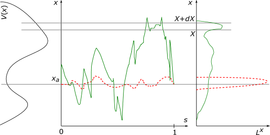
Figure 1: In the middle, two typical paths $x(s\beta\hbar)=x_{a}+\lambda\xi(s)$ are plotted as functions of the dimensionless time $s$. The solid green path, representing a typical trajectory with a high value of $\beta$, exhibits large fluctuations, whereas the dashed red path, corresponding to small $\beta$, stays in the vicinity of the initial and final point $x_{a}$. On the right, two local-time profiles $L(x)$ are shown. The broad one (solid green) arises from the violently fluctuating path $x(s\beta\hbar)$, whereas the narrow one (dashed red) corresponds to the path with small fluctuations. On the left, we depict a generic potential $V(x)$.

and therefore a systematic Wigner–Kirkwood expansion can be readily developed by Taylor-expanding the potential part of the action JizbaZatl .

When $\beta$ is large (i.e., low temperature), the trajectories $x(s\beta\hbar)$ fluctuate heavily around the value $x_{a}$, and the potential term $V$ dominates over the kinetic one. From the statistical physics point of view, the most important contribution to the low temperature behavior of the path integral (4) should come from those paths that spend a sizable amount of time near the global minimum of the potential $V(x)$. For this reason, it is important to be able to keep track of the time which a given path spends in an infinitesimal neighborhood of an arbitrary point $x$.

Let us define, for each Wiener trajectory $x(\tau)$ present in the Feynman path integral (3) the ensuing local time as

$$L^{X}(\tau)\ =\ \int_{0}^{\tau}\!d\tau^{\prime}\ \!\delta\!\left(X-x(\tau^{\prime})\right)\,.$$ (5)

Since the local time $L^{X}(\tau)$ is a functional of the random trajectory $x(\tau^{\prime})$ for $0<\tau^{\prime}<\tau$, it represents a random variable. From the definition (5) we can immediately see that $L^{X}\geq 0$ for all $X\in\mathbb{R}$, $\int_{\mathbb{R}}dX\ \!L^{X}(\tau)=\tau$ and that $L^{X}$ has a compact support. In addition, it can be proved RevuzYor ; Marcus that local-time trajectories $L^{X}$ are, with probability one, continuous curves which (similarly as trajectories in the underlying Wiener process) are nowhere differentiable. In Fig. 1 we depict two examples of representative local-time trajectories. An extensive mathematical discussion of properties of the local time can be found, e.g. in Refs. Marcus ; Borodin .

With the definition (5) the potential part of the Euclidean action can be recast into form $\int_{\mathbb{R}}dX\ \!L^{X}(\beta\hbar)V(X)$. A local-time representation of the Bloch density matrix $\rho(x_{a},x_{b},\beta)$ is then given by

$$\rho(x_{a},x_{b},\beta)\ =\ \int\mathcal{D}L^{x}\ \!\mathcal{W}[L;\beta,x_{a},x_{b}]\ \!\delta\!\left(\int_{\mathbb{R}}dX\ \!L^{X}-\beta\hbar\right)\exp\left[-\frac{1}{\hbar}\int_{\mathbb{R}}dX\ \!L^{X}V(X)\right],$$ (6)

where the PI “sum” is taken over all local-time trajectories $L^{x}$, with $x$ being the independent variable (not to be mistaken with the Wiener trajectory $x(\tau)$). The $\delta$-function enforces the normalization constraint mentioned above. Basically, transition to the local-time description represents a change (or a functional substitution) of stochastic variables $x(\tau)\rightarrow L^{x}(\beta\hbar)$. The weight factor $\mathcal{W}$ appearing in (6) can be formally written in the form

$$\mathcal{W}[L;\beta,x_{a},x_{b}]\ =\ \exp\left[-\frac{1}{\hbar}\int_{0}^{\beta\hbar}\!\!d\tau\ \!\frac{M}{2}\dot{x}^{2}\right]\ \!\det\left(\frac{\delta L^{x}(\beta\hbar)}{\delta x(\tau)}\right)^{-1}\,.$$ (7)

It is a function of $x_{a}$, $x_{b}$ (which are implicitly present in $L^{x}(\beta\hbar)$) and $\beta$, and a functional of the local time $L^{x}$. Of course, these cavalier manipulations do not have more than a heuristic nature, and it is, indeed, a non-trivial task to determine $\mathcal{W}$ directly from (7). For this reason, we will in the following Section tackle this problem indirectly.

IV Local-time representation of path integrals: derivation

In this Section, we present a derivation of the local-time representation of the Bloch density matrix (1). Initially, we limit ourselves to considering the case of the diagonal part, $x_{b}=x_{a}$, and arrive at the key result (16), which expresses the matrix elements in the ensuing Laplace picture with respect to $\beta$. This intermediate outcome is shown to agree with the Sturm–Liouville theory. In the next step, we generalize the latter result to the off-diagonal elements ($x_{b}\neq x_{a}$). The inverse Laplace transform will then yield the sought local-time representation of PI [cf. Eq. (28)].

IV.1 Field-theoretic representation

It follows from the definition (1) that the function $\rho(x_{a},x_{b},\beta)$ satisfies the heat equation

$$\left[\frac{\partial}{\partial\beta}-\frac{\hbar^{2}}{2M}\frac{\partial^{2}}{\partial x_{b}^{2}}+V(x_{b})\right]\rho(x_{a},x_{b},\beta)\ =\ 0\,,$$ (8)

with the initial condition $\rho(x_{a},x_{b},0_{+})=\delta(x_{a}-x_{b})$. This is merely a Wick-rotated ($t\rightarrow-i\hbar\beta$) analogue of the Schrödinger equation. The Feynman–Kac formula Kac1949 ; Feynman1948 ; Friedlin:85 then ensures that the PI (3) can be calculated by solving corresponding parabolic differential equation (8).

In the Laplace picture Eq. (8) takes the form

$$\left[E-\frac{\hbar^{2}}{2M}\frac{\partial^{2}}{\partial x_{b}^{2}}+V(x_{b})\right]\widetilde{\rho}(x_{a},x_{b},E)\ =\ \delta(x_{a}-x_{b})\,,$$ (9)

with $\widetilde{\rho}(x_{a},x_{b},E)=\int_{0}^{\infty}d\beta e^{-\beta E}\rho(x_{a},x_{b},\beta)$. Eq. (9) implies that $\widetilde{\rho}$ is nothing but the Green function of the operator $E+\hat{H}$. With the benefit of hindsight, we represent the Green function $\widetilde{\rho}$ as a path integral over fluctuating fields — so-called functional integral Ramond . This is rather standard strategy in Quantum Field Theory Zinn ; BJV , and in our case it yields

$$\widetilde{\rho}(x_{a},x_{b},E)\ =\ \frac{\int_{\psi(X_{-})=0}^{\psi(X_{+})=0}\mathcal{D}\psi(x)\ \!\psi(x_{a})\psi(x_{b})\ \!e^{-\frac{1}{2}\mathcal{A}^{E}[\psi]}}{\int_{\psi(X_{-})=0}^{\psi(X_{+})=0}\mathcal{D}\psi(x)\ \!e^{-\frac{1}{2}\mathcal{A}^{E}[\psi]}}\,,$$ (10)

where

$$\mathcal{A}^{E}[\psi] \ \equiv\ \int_{X_{-}}^{X_{+}}\!\!\!dx\ \!\psi(x)\left[-\frac{\hbar^{2}}{2M}\frac{d^{2}}{dx^{2}}+V(x)+E\right]\psi(x)$$

$$\ =\ \int_{X_{-}}^{X_{+}}\!\!\!dx\left[\frac{\hbar^{2}}{2M}\psi^{\prime}(x)^{2}+(V(x)+E)\psi(x)^{2}\right],$$ (11)

is the Euclidean action functional of the field-theoretic path integral. The super-index “$E$” in $\mathcal{A}$ indicates the shift in the potential $V(x)$ by the amount $E$. Here, we have confined our quantum-mechanical system within a finite box $[X_{-},X_{+}]$, with $X_{-}\ll\min\{x_{a},x_{b}\}$ and $X_{+}\gg\max\{x_{a},x_{b}\}$. A real scalar field $\psi(x)$ satisfies Dirichlet boundary conditions $\psi(X_{-})=\psi(X_{+})=0$ so as to ensure the validity of the operations being performed.

IV.2 Replica trick

Since we will ultimately want to invert the Laplace transform to regain from $\widetilde{\rho}(x_{a},x_{b},E)$ the original Bloch density matrix $\rho(x_{a},x_{b},\beta)$, we cannot treat the denominator in (10) as an irrelevant normalization constant (which is the usual practice in Quantum Field Theory) but we have to take care of its $E$-dependence. To this end we take advantage of the formula

$$\frac{a}{b}\ =\ \lim_{D\rightarrow 0}ab^{D-1}\,,$$ (12)

which is a simple version of the so-called replica trick. [The usual replica-trick formula (cf. e.g., Ref. Parisi:87 ) can be obtained from (12) by integrating both sides with respect to $b$ and subsequently dividing by $a$.] With the help of (12) we can rewrite (10) as a multidimensional functional integral

$$\widetilde{\rho}(x_{a},x_{b},E)\ =\ \lim_{D\rightarrow 0}\frac{2}{D}\int_{\bm{\psi}(X_{-})=\bm{0}}^{\bm{\psi}(X_{+})=\bm{0}}\!\!\mathcal{D}\bm{\psi}(x)\ \!\bm{\psi}(x_{a})\cdot\bm{\psi}(x_{b})\ \!e^{-\sum_{\sigma=1}^{D}\mathcal{A}^{E}[\psi_{\sigma}]}\,,$$ (13)

where the multiplet ${\bm{\psi}}=(\psi_{1},\ldots,\psi_{D})$ is a $D$-component “replica” field in $1+0$ dimensions, $\bm{\psi}(x_{a})\cdot\bm{\psi}(x_{b})$ denotes the scalar product $\sum_{\sigma=1}^{D}\psi_{\sigma}(x_{a})\psi_{\sigma}(x_{b})$, and we have rescaled the fields by a factor of $\sqrt{2}$ in passing. The factor $1/D$ results from a PI generalization of the well know mean-value identity $\langle x_{i}\ \!y_{i}\rangle=\langle{\bf{x}}\cdot{\bf{y}}\rangle/D$ valid for any two vectors in $D$-dimensional statistically isotropic environments.

As a side remark, note that we may now invert the Laplace transform, using the trivial identity

$$\int_{0}^{\infty}d\beta\ \!e^{-\beta E}\delta(\beta-c)\ =\ e^{-cE}\;\;\;\,\,\,\,\mbox{for}\;\;\;\;c\ >\ 0\,,$$ (14)

to obtain the representation

$$\rho(x_{a},x_{b},\beta)\ =\ \lim_{D\rightarrow 0}\frac{2}{D}\int_{\bm{\psi}(X_{-})=\bm{0}}^{\bm{\psi}(X_{+})=\bm{0}}\!\!\mathcal{D}\bm{\psi}\ \!\ \!\bm{\psi}(x_{a})\cdot\bm{\psi}(x_{b})\ \!\ \!\delta\!\left(\int_{X_{-}}^{X_{+}}\!\!\!\bm{\psi}(x)^{2}dx-\beta\right)e^{-\sum_{\sigma=1}^{D}\mathcal{A}^{E=0}[\psi_{\sigma}]}\,.$$ (15)

Upon scaling $\bm{\psi}\rightarrow\sqrt{\beta}\bm{\psi}$, this agrees with the formula (2.9) in Ref. Luttinger1982 . Though the result (15) generalizes to arbitrary number of dimensions of the $x$-space, i.e., $x\in\mathbb{R}^{d}$, our further development will be illustrated (for simplicity’s sake) only on the one-dimensional case.

IV.3 Connection with radial harmonic oscillator

In order to derive the weight factor $\mathcal{W}$ (cf. Eq. (7)) we have arrived at the representation (15) with $D$ replica fields. This form is still not very transparent, and a further simplification step is needed to get rid of an explicit dependence of the measure on $D$. To this end, we note that $\sum_{\sigma=1}^{D}\mathcal{A}^{E}[\psi]$ is in fact the action of a $D$-dimensional harmonic oscillator with the “time” variable $x$, “position” variable $\psi$, mass $\hbar^{2}/M$, and time-dependent “frequency” $V(x)+E$. Considering for a moment only diagonal matrix elements, $x_{b}=x_{a}$, spherical symmetry in the replica field space allows to reduce the path integral (13) to its radial part. Due to the boundary conditions, $\bm{\psi}(X_{-})=\bm{\psi}(X_{+})=\bm{0}$, only the zero-angular-momentum ($s$-wave) contribution is non-vanishing (generally a weighted sum over radial PI’s with different angular momenta would be required). This will be rigorously justified at the end of this Section. The corresponding radial PI representation for (13) reads Grosche ; Zinn ; Kleinert

$$\widetilde{\rho}(x_{a},x_{a},E)\ =\ \lim_{D\rightarrow 0}\frac{2}{D\Omega(D)}\lim_{\eta_{\pm}\rightarrow 0}(\eta_{-}\eta_{+})^{\frac{1-D}{2}}\int_{\eta(X_{-})=\eta_{-}}^{\eta(X_{+})=\eta_{+}}\!\!\mathcal{D}\eta(x)\ \!\eta^{2}(x_{a})\ \!e^{-A_{D}^{E}[\eta]}\,.$$ (16)

Here, the radial part $\eta\equiv\sqrt{\bm{\psi}^{2}}$ of the $D$-dimensional replica field $\bm{\psi}$ is always non-negative, i.e., $\eta(x)\geq 0$; the area of a unit sphere in $D$ dimensions, $\Omega(D)=2\pi^{D/2}/\Gamma(D/2)$, may be replaced by its small-$D$ asymptotic form $\Omega(D)\sim D$; and $\eta_{\pm}$ have been introduced to regularize the origin of the $\bm{\psi}$-space. The new action functional

$$\mathcal{A}_{D}^{E}[\eta]\ \equiv\ \mathcal{A}^{E}[\eta]\ +\ \int_{X_{-}}^{X_{+}}\!\!dx\ \!\frac{M}{\hbar^{2}}\frac{(D\!-\!1)(D\!-\!3)}{8\eta^{2}(x)}\,,$$ (17)

is the Euclidean action functional of the radial harmonic oscillator Kleinert ; Grosche ; Steiner . It contains an additional centrifugal potential term (Edwards–Gulyaev or Langer term E-G-64 ; Kleinert ; Inomata:66 ), which emerges from Bessel function $I_{D/2-1}$ present in the finite sliced form of the radial PI (16). At this point we should stress that in contrast to the quantum-mechanical radial PI, one can use safely the asymptotic expansion for the Bessel function $I_{D/2-1}$ (see, e.g. Ref. Gradshteyn ):

$$I_{\mu}(y_{j})\ \sim\ \frac{1}{\sqrt{2\pi y_{j}}}\ \!e^{y_{j}-(\mu^{2}-1/4)/2y_{j}},\;\;\;\;\;\;\;\;\;(|y_{j}|\gg 1,\;\mbox{Re}[y_{j}]>0)\,,$$

$$y_{j}\ =\ (m/\varepsilon\hbar)r_{j}r_{{j-1}}\,,$$ (18)

in the Euclidean PI sliced form. Here the infinitesimal “time” slice $\varepsilon$ is related to the number of slices $N$ via the relation $\varepsilon=\hbar\beta/N$. In quantum mechanic this is a problematic step because (18) requires $\mbox{Re}[y_{j}]>0$ while there $\mbox{Re}[y_{j}]=\mbox{Re}[(m/i\varepsilon\hbar)r_{j}r_{{j-1}}]=0$.

Fortunately, the PI for radial harmonic oscillator is exactly solvable even in the case of $x$-dependent oscillator frequency. The solution reads Grosche

$$(\eta_{2}x_{2}|\eta_{1}x_{1})_{D}\ \equiv \int_{\eta(x_{1})=\eta_{1}}^{\eta(x_{2})=\eta_{2}}\!\!\!\mathcal{D}\eta(x)\exp\left\{-\int_{x_{1}}^{x_{2}}\!\!\!dx\left[\frac{\hbar^{2}}{2M}\eta^{\prime 2}+(V(x)+E)\eta^{2}+\frac{M}{\hbar^{2}}\frac{(D\!-\!1)(D\!-\!3)}{8\eta^{2}}\right]\right\}$$ (19)

$$= \ \frac{\hbar^{2}}{M}\frac{\sqrt{\eta_{1}\eta_{2}}}{G(x_{1})}I_{D/2-1}\left(\frac{\hbar^{2}}{M}\frac{\eta_{1}\eta_{2}}{G(x_{1})}\right)\exp\left[-\frac{\hbar^{2}}{2M}\left(\frac{F^{\prime}(x_{2})}{F(x_{2})}\eta_{2}^{2}-\frac{G^{\prime}(x_{1})}{G(x_{1})}\eta_{1}^{2}\right)\right].$$

The functions $F(x)$ and $G(x)$ are two independent solutions of the differential equation

$$\left[\hat{H}+E\right]y(x)\ =\ \left[-\frac{\hbar^{2}}{2M}\frac{d^{2}}{dx^{2}}+V(x)+E\right]y(x)\ =\ 0\,,$$ (20)

with the initial conditions $F(x_{1})=0$ and $F^{\prime}(x_{1})=1$, and $G(x_{2})=0$ and $G^{\prime}(x_{2})=-1$. In addition, the Wronskian $W(F,G)\equiv F(x)G^{\prime}(x)-F^{\prime}(x)G(x)$ is independent of $x$, as can be proved by differentiation and by using the fact that $F$ and $G$ both satisfy Eq. (20). By equating the values of $W(F,G)$ at points $x_{1}$ and $x_{2}$, and taking into account the initial conditions for $F$ and $G$, we find a useful identity $F(x_{2})=G(x_{1})$.

Now, the PI in (16) can be sliced at point $x_{a}$, and expressed as

$$\widetilde{\rho}(x_{a},x_{a},E)\ =\ \int_{0}^{\infty}\!d\eta_{a}\ \!(\eta_{+}X_{+}|\eta_{a}x_{a})_{D}\ \!\eta_{a}^{2}\ \!(\eta_{a}x_{a}|\eta_{-}X_{-})_{D}\,.$$ (21)

The limits in Eq. (16) are readily carried out with the help of the asymptotic formulas $I_{D/2-1}(z)~{}\approx~{}(z/2)^{D/2-1}/\Gamma(D/2)$, and $\Gamma(z)~{}\approx~{}1/z$, valid for $z\rightarrow 0_{+}$. Subsequent integration over $\eta_{a}$ brings (16) to form

$$\widetilde{\rho}(x_{a},x_{a},E)\ =\ -\frac{2M}{\hbar^{2}}\frac{F_{1}(x_{a})G_{2}(x_{a})}{F_{1}(x_{a})G^{\prime}_{2}(x_{a})-F^{\prime}_{1}(x_{a})G_{2}(x_{a})}\,,$$ (22)

where $F_{1}(x)$ solves Eq. (20) with initial conditions $F_{1}(X_{-})=0$ and $F_{1}^{\prime}(X_{-})=1$, and $G_{2}(x)$ solves the same equation with $G_{2}(X_{+})=0$ and $G_{2}^{\prime}(X_{+})=-1$. The denominator in (22) is the Wronskian $W(F_{1},G_{2})$. The full derivation is given in Appendix A.

Although rather explicit, Eq. (22) is not well suited for the Laplace transform inversion, since functions $F(x)$ and $G(x)$ contain $E$ in a non-trivial way, which, in addition, significantly hinges on the actual form of $V(x)$. For formal manipulations it is still better the employ the PI representation (16). For instance, using Eq. (14) we can easily invert the Laplace transform to return from $E$ back to the $\beta$-variable, namely

$$\mbox{}\rho(x_{a},x_{a},\beta)=\lim_{D\rightarrow 0}\frac{2}{D^{2}}\lim_{\eta_{\pm}\rightarrow 0}(\eta_{-}\eta_{+})^{\frac{1-D}{2}}\!\!\int_{\eta(X_{-})=\eta_{-}}^{\eta(X_{+})=\eta_{+}}\!\!\!\mathcal{D}\eta(x)\ \!\eta^{2}(x_{a})\ \!\delta\!\left(\int_{X_{-}}^{X_{+}}\!\!\!\!\!\eta^{2}dx-\beta\right)\!e^{-A_{D}^{E=0}[\eta]}\,.$$ (23)

Note that we have utilized the asymptotic form $\Omega(D)\sim D$ which holds for $D\ll 1$. We shall see shortly that (23) can be straightforwardly related to the local-time PI representation of the Boltzmann density matrix.

Let us finally comment on the higher-angular-momentum terms which, as claimed, should not contribute to the expression (16). For arbitrary angular momentum $\ell\geq 0$, we employ formula (19) with a slight modification $D\rightarrow D+2\ell$. Now, for example, in the limit $\eta_{-}\rightarrow 0$, this goes like $(\eta_{a}x_{a}|\eta_{-}X_{-})_{D+2\ell}\propto\eta_{-}^{\ell+D/2-1/2}$, which, multiplied by the prefactor $\eta_{-}^{1/2-D/2}$, implies the behavior $\sim\eta_{-}^{\ell}$. That is, only the ($\ell=0$)-term can give a non-vanishing contribution.

IV.4 Connection with the Sturm–Liouville problem

Consider again Eq. (9) and a finite interval $x\in[X_{-},X_{+}]$. The corresponding Green function of the operator $\hat{H}+E$ can be easily constructed (at least formally) with the help of the Sturm–Liouville theory Vladimirov ; Zettl . An immediate consequence of the latter is that for $x_{a}<x_{b}$ the Green function has the form

$$\widetilde{\rho}(x_{a},x_{b},E)\ =\ -\frac{2M}{\hbar^{2}}\frac{F(x_{a})G(x_{b})}{W(F,G)}\,,$$ (24)

where the functions $F(x)$ and $G(x)$ satisfy Eq. (20) with the initial conditions $F(X_{-})=0$ and $F^{\prime}(X_{-})=1$, and $G(X_{+})=0$ and $G^{\prime}(X_{+})=-1$, respectively. In addition, the above Green function should be symmetric due to the Hermitian nature of $\hat{H}$.

The Sturm–Liouville theory ensures that the solution to the second-order differential equation (20) is unique, when specifying the values of $y(x_{0})$ and $y^{\prime}(x_{0})$ at some point $x_{0}$. Therefore, the functions $F$ and $G$ must coincide with $F_{1}$ and $G_{2}$ of Eq. (22), and the diagonal part of (24), i.e. $\widetilde{\rho}(x_{a},x_{a},E)$, reduces to expression (22). This is an important consistency check of our representation (16).

IV.5 Extension to off-diagonal matrix elements

Let us now generalize the PI representation (16) to the full Bloch density matrix, i.e., we wish to include also the off-diagonal matrix elements, $x_{b}\neq x_{a}$. If we go back to the replica representation (13), we realize that the requirement $x_{b}\neq x_{a}$ spoils rotational symmetry in the replica field space, and thus precludes straightforward reduction to a radial path integral. Instead of refining the reduction procedure, we simply make a guess, which, as we prove in Appendix A, coincides with the well-established Sturm–Liouville Formula (24). Our guess is based on mathematical results presented in Borodin . In particular, we claim that the extension of the representation (16) to off-diagonal matrix elements should read

$$\widetilde{\rho}(x_{a},x_{b},E)=\lim_{D\rightarrow 0}\frac{2}{D^{2}}\lim_{\eta_{\pm}\rightarrow 0}(\eta_{-}\eta_{+})^{\frac{1-D}{2}}\int_{\eta(X_{-})=\eta_{-}}^{\eta(X_{+})=\eta_{+}}\!\!\!\mathcal{D}\eta(x)\ \!\eta(x_{a})\eta(x_{b})\ \!e^{-\mathcal{A}^{E}_{\Delta}[\eta]}\,,$$ (25)

with the action functional

$$\mathcal{A}^{E}_{\Delta}[\eta]\ \equiv\ \mathcal{A}^{E}[\eta]\ +\ \int_{X_{-}}^{X_{+}}\!\!dx\ \!\frac{M}{\hbar^{2}}\frac{\Delta(x)}{8\eta^{2}(x)}\,,$$ (26)

where $\mathcal{A}^{E}[\eta]$ is defined in Eq. (IV.1), and $\Delta(x)$ is a piecewise constant function

$$\Delta(x)=\begin{cases}-1&{\rm for~{}}x\in[x_{a},x_{b}]\\ (D-1)(D-3)&{\rm otherwise}.\end{cases}$$ (27)

At this point we can invert the Laplace transform with the help of Eq. (14). As a result, we obtain the sought local-time PI representation of the Bloch density matrix (1), namely

$$\rho(x_{a},x_{b},\beta)=\lim_{D\rightarrow 0}\frac{2}{D^{2}}\lim_{\eta_{\pm}\rightarrow 0}(\eta_{-}\eta_{+})^{\frac{1-D}{2}}\int_{\eta(X_{-})=\eta_{-}}^{\eta(X_{+})=\eta_{+}}\!\!\!\mathcal{D}\eta\ \!\ \!\eta(x_{a})\eta(x_{b})\ \!\delta\!\left(\int_{X_{-}}^{X_{+}}\!\!\!\!\!\eta^{2}dx-\beta\right)e^{-\mathcal{A}^{E=0}_{\Delta}[\eta]}\,.$$ (28)

Here, integrations over $\eta(x)$ run from $0$ to $+\infty$, i.e., the paths $\eta(x)$ are non-negative. Comparing this result with the anticipated heuristic form (6), we can identify $\eta^{2}(x)=L^{X}(\beta\hbar)/\hbar$. Representation (28) allows us to identify the weight factor (7) with

$$\mathcal{W}_{D}[\eta;\beta,x_{a},x_{b}]\ =\ \frac{2}{D^{2}}(\eta_{-}\eta_{+})^{\frac{1-D}{2}}\eta(x_{a})\eta(x_{b})\exp\left\{-\int_{X_{-}}^{X_{+}}\!\!\!dx\left[\frac{\hbar^{2}}{2M}{\eta^{\prime}}^{2}+\frac{M}{\hbar^{2}}\frac{\Delta(x)}{8\eta^{2}}\right]\right\}.$$ (29)

Contrary to expectation, the right-hand-side of this expression does not depend on $\beta$. Sub-index $D$ in $\mathcal{W}_{D}$ indicates that the weight factor must be regularized when we pull it out of the PI (28). By analogy with quantum mechanics one can represent (28) in the discretized time-sliced form. In such a case the weight $\mathcal{W}_{D}$ would be a product of terms involving the Bessel functions $I_{D/2-1}$, if $\Delta(x)=(D-1)(D-3)$, or $I_{0}$, if $\Delta(x)=-1$ (see Ref. Grosche ).

Last but not least, expressions (28)-(29) indicate that the square root of $L^{X}$ is (at least from physicist’s point of view) more convenient variable to describe local-time trajectories than $L^{X}$ alone.

V Functionals of the local time

Formula (28) provides a way of rewriting the PI (3) in terms of the local time. In this Section, we consider more general scenario, in which the initial path integral is of the form

$$\bar{F}(x_{a},x_{b},\beta)\ \equiv\ \int_{x(0)=x_{a}}^{x(\beta\hbar)=x_{b}}\!\!\!\mathcal{D}x(\tau)\ \!F[L]\ \!\exp\left\{-\frac{1}{\hbar}\int_{0}^{\beta\hbar}\!\!\!d\tau\left[\frac{M}{2}\dot{x}^{2}+V(x)\right]\right\},$$ (30)

where $F$ is an arbitrary functional of the local time $L^{X}(\beta\hbar)$, which itself is (as seen in Section III) a functional of the paths $x(\tau)$. Relation (30) represents a local-time analog of the Feynman–Matthews–Salam formula LvW ; BJV .

To bring it into more manageable form, we may observe that for any $X$, the action of $L^{X}$ in the PI (30) can be taken over by the functional derivative $-\hbar\delta/\delta V(X)$, acting on the exponential. This becomes transparent after rewriting the potential part as $\int_{0}^{\beta\hbar}\!d\tau\ \!V(x(\tau))=\int_{\mathbb{R}}dX\ \!V(X)L(X)$. The entire functional $F[L]$ can be therefore pulled out of the path integral, which then allows to write

$$\bar{F}(x_{a},x_{b},\beta)\ =\ F\left[-\hbar\frac{\delta}{\delta V}\right]\rho(x_{a},x_{b},\beta)\,.$$ (31)

When we employ the local-time representation of PI for $\rho(x_{a},x_{b},\beta)$ (cf. Eq. (28)), each functional derivative $-\hbar\delta/\delta V(x)$ will produce the term $\hbar\eta^{2}(x)$. In such a way $\bar{F}$ can be written as

$$\mbox{}\bar{F}(x_{a},x_{b},\beta)$$

$$\mbox{}=\ \lim_{D\rightarrow 0}\frac{2}{D^{2}}\lim_{\eta_{\pm}\rightarrow 0}(\eta_{-}\eta_{+})^{\frac{1-D}{2}}\int_{\eta(X_{-})=\eta_{-}}^{\eta(X_{+})=\eta_{+}}\!\!\!\!\!\mathcal{D}\eta\ \!\ \!\eta(x_{a})\eta(x_{b})\ \!\delta\!\left(\int_{X_{-}}^{X_{+}}\!\!\!\!\!\eta^{2}dx-\beta\right)F[\hbar\eta^{2}]e^{-\mathcal{A}^{E=0}_{\Delta}[\eta]}\,,$$ (32)

where, strictly speaking, the functional $F[\cdots]$ is regularized in such a way that it depends on $L^{X}$ only for $X\in[X_{-},X_{+}]$, and $X_{\pm}$ are sent to $\pm\infty$ only at the end of the calculation.

First, let us make the simple observation that the formula (32) reduces to (28) for the choice $F[L]=1$. One of the most important mean values of a local-time functional, as evaluated with Eq. (32), is the mean of $\exp(-\int_{\mathbb{R}}{dXL^{X}j(X)})$ which gives the moment-generating functional. The local-time moment structure is particularly pertinent in various perturbative expansions, including low- and high-temperature expansions (see Section VI). Another important example, namely the case of a one-point distribution function will be discussed in the following subsection.

In passing we should note, that should we have started from (15) and repeated the above procedure, an analog of Eq. (32) for higher-dimensional spaces, $x\in\mathbb{R}^{d}$, could be easily obtained. This would include the $D$-dimensional replica field $\bm{\psi}$ in the $d$-dimensional Euclidean configuration space.

V.1 Example: One-point distribution function at the origin

Simple, though quite important consequence of Eq. (32) is that it readily provides the $N$-point distribution functions of the local time. This is achieved when we set $F[L]=\prod_{n=1}^{N}\delta(L^{X_{n}}-L_{n})$. In order to see what is involved let us now illustrate the calculation for $N=1$ (with $L_{1}\equiv L$). Our discussion will be greatly simplified by considering only a free particle (i.e., $V(x)=0$) that starts and ends at the origin, i.e., $x_{a}=x_{b}=0$. This corresponds to a stochastic process known as Brownian bridge. Our goal is to derive the one-point distribution function, denoted $p(L;\beta)$, of the local time at $X=0$. We define $p(L;\beta)$ by Eq. (30) with $F[L]=\delta(L^{0}-L)$, and calculate it from the representation (32) as follows.

In the Laplace picture, $\widetilde{p}(L;E)=\int_{0}^{\infty}\!d\beta e^{-\beta E}p(L;\beta)$, the path integral (32) can be sliced at $x_{a}=x_{b}=0$ so that

$$\widetilde{p}(L;E)=\lim_{D\rightarrow 0}\frac{2}{D^{2}}\lim_{\eta_{\pm}\rightarrow 0}(\eta_{-}\eta_{+})^{\frac{1-D}{2}}\int_{0}^{\infty}\!\!\!d\eta_{0}\ \!\eta_{0}^{2}\ \!\delta(\hbar\eta_{0}^{2}-L)(\eta_{+}X_{+}|\eta_{0}~{}0)_{D}(\eta_{0}~{}0|\eta_{-}X_{-})_{D}\,.$$ (33)

The $\eta_{0}$-integration can be done easily by realizing that $\delta(\hbar\eta_{0}^{2}-L)=\delta(\eta_{0}-\sqrt{L/\hbar})/2\sqrt{\hbar L}$. Furthermore, the limits in $\eta_{\pm}$ and $D$ can be carried out with the help of formulas (59) and (60) from Appendix A. Consequently, we obtain

$$\widetilde{p}(L;E)=\exp\left[-\frac{L\hbar^{2}}{2M}\left(\frac{F^{\prime}_{1}(0)}{F_{1}(0)}-\frac{G^{\prime}_{3}(0)}{G_{3}(0)}\right)\right],$$ (34)

where, for the free-particle case, $F_{1}(x)=\sinh[\sqrt{2ME/\hbar^{2}}(x-X_{-})]/\sqrt{2ME/\hbar^{2}}$, and $G_{3}(x)=\sinh[\sqrt{2ME/\hbar^{2}}(X_{+}-x)]/\sqrt{2ME/\hbar^{2}}$, as one can straightforwardly verify. In the limit $X_{\pm}\rightarrow\pm\infty$, Eq. (34) reduces to

$$\widetilde{p}(L;E)=e^{-\sqrt{2\hbar^{2}E/M}L},$$ (35)

and its inverse-Laplace transform yields

$$p(L;\beta)=\frac{L\exp\left(-\frac{L^{2}\hbar^{2}}{2\beta M}\right)}{\sqrt{2\pi M\beta^{3}/\hbar^{2}}}\,.$$ (36)

We stress that $p(L;\beta)$ thus obtained is, in fact, the (unnormalized ) joint probability density for stochastic events “$x(0)=0\rightsquigarrow x(\beta\hbar)=0$” and “$L^{0}=L$”. By Bayes’ theorem of the probability calculus, the desired conditional probability density $p[L^{0}\!=\!L|x(0)\!=\!0\!\rightsquigarrow\!x(\beta\hbar)\!=\!0]$ is obtained from (36) by dividing $p(L;\beta)$ by the Brownian-bridge probability density $p[x(0)\!=\!0\!\rightsquigarrow\!x(\beta\hbar)\!=\!0]$, which is (omitting again normalization) $(2\pi\beta\hbar^{2}/M)^{-1/2}$ (see, e.g., Ref. FeynmanHibbs ). Normalization factors mutually cancel in the fraction and we arrive at

$$p[L^{0}\!=\!L|x(0)\!=\!0\!\rightsquigarrow\!x(\beta\hbar)\!=\!0]\ =\ \frac{\hbar^{2}L\exp\left(-\frac{L^{2}\hbar^{2}}{2\beta M}\right)}{{\beta M}}\,,$$ (37)

which is clearly normalized to $1$. One can proceed along the same lines also in more complicated higher-dimensional ($N>1$) cases. Our result agrees with the one found through other means in Ref. Borodin .

VI Asymptotic behavior of the Bloch density matrix

A compelling feature of the local-time representation (28) is that it naturally captures both small- and large-$\beta$ asymptotic regimes. This should be compared with the Feynman–Kac PI representation (3), which is typically suitable only for the small-$\beta$ (i.e., large-temperature) analysis. The latter is epitomized either by WKB approximation Zinn ; Kleinert or Wigner–Kirkwood expansion JizbaZatl . In the large-$\beta$ (small-temperature) limit, the spectral representation of the Gibbs operator, $e^{-\beta\hat{H}}=\sum_{n}e^{-\beta E_{n}}\left|\phi_{n}\right\rangle\left\langle\phi_{n}\right|$, reduces the Bloch density matrix to the ground-state contribution

$$\rho(x_{a},x_{b},\beta)\ \overset{\beta\rightarrow\infty}{\sim}\ e^{-\beta E_{gs}}\ \!\psi_{gs}^{*}(x_{a})\psi_{gs}(x_{b})\,,$$ (38)

that is not evident from the Feynman–Kac PI representation Note-1 . In connection with Eq. (38) it is useful to remind that in $d=1$ the discrete bound states can all be chosen to be real Messiah , so that the Bloch density matrix is real and symmetric and can be written in the form

$$\rho(x_{a},x_{b},\beta)\ =\ \sum_{n=0}e^{-\beta E_{n}}\psi_{n}(x_{a})\psi_{n}(x_{b})\ \overset{\beta\rightarrow\infty}{\sim}\ e^{-\beta E_{gs}}\ \!\psi_{gs}(x_{a})\psi_{gs}(x_{b})\,.$$ (39)

Let us first comment on the small-$\beta$ regime of the local-time representation, assuming $x_{b}=x_{a}$ for simplicity. This case was discussed in detail in our previous article JizbaZatl . There one should first Taylor-expand the potential $V(x)$ around the point $x_{a}$, and then expand the exponential part containing the structure $\int\eta^{2}(x)O(x-x_{a})dx$, where

$$O(x-x_{a})\ =\ \beta\sum_{m\neq 0}\frac{V^{(m)}(x_{a})}{m!}[\lambda(x-x_{a})]^{m}\,.$$ (40)

After the term $e^{-\beta V(x_{a})}/\lambda$ is factored out of the integral, the individual summands of the ensuing series are of the form (32) with the potential $V(x)=0$, and functional $F[L]\propto\prod_{n}L^{x_{n}}/\hbar$. The latter can be related to the power expansion in $\beta$ presented in JizbaZatl through the equality of representations (30) and (32). The whole Bloch density matrix (containing also off-diagonal elements) can be treated similarly in a full analogy with Ref. JizbaZatl .

The large-$\beta$ expansion of Eq. (28) can be conveniently studied after rescaling $\eta\rightarrow\sqrt{\beta}\eta$, in which case we can write

$$\rho(x_{a},x_{b},\beta) = \ \lim_{D\rightarrow 0}\frac{2}{D^{2}}\lim_{\eta_{\pm}\rightarrow 0}(\eta_{-}\eta_{+})^{\frac{1-D}{2}}\int_{\eta(X_{-})=\eta_{-}}^{\eta(X_{+})=\eta_{+}}\mathcal{D}\eta(x)\ \!\ \!\eta(x_{a})\eta(x_{b})$$ (41)

$$\times \ \delta\!\left(\int_{X_{-}}^{X_{+}}\!\!\!\eta^{2}dx-1\right)\exp\left\{-\int_{X_{-}}^{X_{+}}\!\!\!dx\left[\frac{\beta\hbar^{2}}{2M}{\eta^{\prime}}^{2}+\beta V(x)\eta^{2}+\frac{M}{\beta\hbar^{2}}\frac{\Delta(x)}{8\eta^{2}}\right]\right\}$$

$$= \ \lim_{D\rightarrow 0}\frac{2}{D^{2}}\lim_{\eta_{\pm}\rightarrow 0}(\eta_{-}\eta_{+})^{\frac{1-D}{2}}\frac{\beta\delta^{2}}{\delta J(x_{a})\delta J(x_{b})}\int_{c-i\infty}^{c+i\infty}\frac{d\kappa}{2\pi i}\int_{\eta(X_{-})=\eta_{-}}^{\eta(X_{+})=\eta_{+}}\mathcal{D}\eta(x)$$

$$\times \ \exp\left\{-\beta\left[\int_{X_{-}}^{X_{+}}\!\!\!dx\left(\frac{\hbar^{2}}{2M}{\eta^{\prime}}^{2}+V(x)\eta^{2}-\kappa\eta^{2}\right)+\kappa\right]\right\}$$

$$\times \ \left.\exp\left\{-\int_{X_{-}}^{X_{+}}\!\!\!dx\left[\frac{M}{\beta\hbar^{2}}\frac{\Delta(x)}{8\eta^{2}}+J\eta\right]\right\}\right|_{J=0},$$

where $c$ is an arbitrary real number. With the method of images Kleinert ; Grosche ; Schulman:97 we can rewrite the radial PI involved as a superposition of two genuine one-dimensional PI’s Steiner

$$\mbox{}\int_{\eta(X_{-})=\eta_{-}}^{\eta(X_{+})=\eta_{+}}\mathcal{D}^{R}\eta(x)\exp\left\{-\beta\left[\langle\eta|\hat{H}|\eta\rangle-\kappa\left(\langle\eta|\eta\rangle-1\right)\right]-\langle J|\eta\rangle\right\}\exp\left[-\int_{X_{-}}^{X_{+}}dx\ \!\frac{M}{\beta\hbar^{2}}\frac{\Delta(x)}{8\eta^{2}}\right]_{\!R}$$

$$\mbox{\hskip 28.45274pt}=\ \int_{\eta(X_{-})=\eta_{-}}^{\eta(X_{+})=\eta_{+}}\mathcal{D}\eta(x)\exp\left\{-\beta\left[\langle\eta|\hat{H}|\eta\rangle-\kappa\left(\langle\eta|\eta\rangle-1\right)\right]-\langle J||\eta|\rangle\right\}$$

$$\mbox{\hskip 39.83385pt}\times\ \exp\left[-\int_{X_{-}}^{X_{+}}dx\ \!\frac{M}{\beta\hbar^{2}}\frac{\Delta(x)}{8\eta^{2}}\right]$$

$$\mbox{\hskip 28.45274pt}-\ \cos(\pi D/2)\int_{\eta(X_{-})=-\eta_{-}}^{\eta(X_{+})=\eta_{+}}\mathcal{D}\eta(x)\exp\left\{-\beta\left[\langle\eta|\hat{H}|\eta\rangle-\kappa\left(\langle\eta|\eta\rangle-1\right)\right]-\langle J||\eta|\rangle\right\}$$

$$\mbox{\hskip 39.83385pt}\times\ \exp\left[-\int_{X_{-}}^{X_{+}}dx\ \!\frac{M}{\beta\hbar^{2}}\frac{\Delta(x)}{8\eta^{2}}\right],$$ (42)

where Dirac’s notation was employed. A few comments are in order about the right-hand-side of the above relation. First, it should be noticed the presence of the parity-even terms $\langle J||\eta|\rangle$ in PI’s. Second, PI’s differ by their respective Dirichlet boundary conditions. Third, the super-index “$R$” was used to stress the restricted nature of the fluctuations in the radial PI measure while the measure without “$R$” represents a usual one-dimensional PI measure, i.e.

$$\mathcal{D}^{R}\eta(x)\ \dot{=}\ \lim_{N\rightarrow\infty}\left(\frac{\beta\hbar^{2}}{2\pi\varepsilon M}\right)^{\!\!N/2}\prod_{k=1}^{N-1}\int_{0}^{\infty}d\eta_{k},\;\;\;\;\mathcal{D}\eta(x)\ \dot{=}\ \lim_{N\rightarrow\infty}\left(\frac{\beta\hbar^{2}}{2\pi\varepsilon M}\right)^{\!\!N/2}\prod_{k=1}^{N-1}\int_{-\infty}^{\infty}d\eta_{k}\,.$$ (43)

Here “$\dot{=}$” denotes De Witt’s “equivalence” symbol DeWitt . Finally, the correct time-sliced form of the exponential with the centrifugal potential is (cf. e.g., Refs. Kleinert ; Steiner )

$$\exp\left[-\int_{X_{-}}^{X_{+}}dx\ \!\frac{M}{\beta\hbar^{2}}\frac{\Delta(x)}{8\eta^{2}}\right]_{\!R}\ \dot{=}\ \lim_{N\rightarrow\infty}\prod_{k=1}^{N}\sqrt{2\pi\frac{\beta\hbar^{2}}{M}\frac{\eta_{k}\eta_{k-1}}{\varepsilon}\tilde{\Delta}_{k}}\ \!\exp\left(-\frac{\beta\hbar^{2}}{M}\frac{\eta_{k}\eta_{k-1}}{\varepsilon}\tilde{\Delta}_{k}\right)I_{\frac{D-2}{2}}\left(\frac{\beta\hbar^{2}}{M}\frac{\eta_{k}\eta_{k-1}}{\varepsilon}\tilde{\Delta}_{k}\right),$$

$$\exp\left[-\int_{X_{-}}^{X_{+}}dx\ \!\frac{M}{\beta\hbar^{2}}\frac{\Delta(x)}{8\eta^{2}}\right]\ \dot{=}\ \lim_{N\rightarrow\infty}\prod_{k=1}^{N}\psi_{\frac{D-2}{2}}\left(-\frac{\beta\hbar^{2}}{M}\frac{|\eta_{k}\eta_{k-1}|}{\varepsilon}\tilde{\Delta}_{k}\right),$$ (44)

with

$$\tilde{\Delta}_{k}\ \equiv\ \tilde{\Delta}(x_{k})\ =\ \begin{cases}-(D-1)(D-3)&{\rm for~{}}x_{k}\in[x_{a},x_{b}]\\ 1&{\rm otherwise},\end{cases}$$ (45)

and (see, e.g., Refs. Steiner ; Dinge )

$$\psi_{p}(x)\ =\ \frac{e^{x}}{\sin(\pi p)}\sqrt{\frac{\pi x}{2}}\left[I_{-p}(x)-I_{p}(x)\right]\ =\ e^{x}\sqrt{\frac{2x}{\pi}}K_{p}(x)\,.$$ (46)

[$I_{p}$ and $K_{p}$ are the modified Bessel functions of the first and the second kind, respectively.] In cases when $x\gg 1$ meaning that $|\eta_{k}\eta_{k-1}|\gg\varepsilon$ (e.g., “typical situation” for very fine time slicings) the asymptotic form of $\psi_{p}(-x)\sim 1+(1-4p^{2})/8x+{\mathcal{O}}(1/x^{2})$ holds. With help of the preceding asymptotic behavior one obtains

$$\prod_{k=1}^{N}\psi_{\frac{D-2}{2}}\left(-\frac{\beta\hbar^{2}}{M}\frac{|\eta_{k}\eta_{k-1}|}{\varepsilon}\tilde{\Delta}_{k}\right)\ \sim \ \prod_{k=1}^{N}\left[1-\frac{M}{\beta\hbar^{2}}\frac{(D-3)(D-1)}{8|\eta_{k}\eta_{k-1}|\tilde{\Delta}_{k}}\ \!\varepsilon+{\mathcal{O}}(\varepsilon^{2})\right]$$ (47)

$$\sim \ \prod_{k=1}^{N}\exp\left[-\frac{M}{\beta\hbar^{2}}\frac{\Delta_{k}}{8|\eta_{k}\eta_{k-1}|}\ \!\varepsilon+{\mathcal{O}}(\varepsilon^{2})\right]$$

$$\sim \ \exp\left[-\int_{X_{-}}^{X_{+}}dx\ \!\frac{M}{\beta\hbar^{2}}\frac{\Delta(x)}{8\eta^{2}}\right].$$

Potential singularities of the integral at $\eta=0$ can be regularized, e.g., by a principal value prescription. Unfortunately, the formula (47) cannot be directly used in our case because the boundary values $\eta_{-}$ and $\eta_{+}$ are arbitrarily close to zero, and hence the assumed asymptotic behavior for $\psi_{p}$ is not fulfilled. This situation can be rectified by factorizing out the problematic boundary points as

$$\prod_{k=1}^{N}\psi_{\frac{D-2}{2}}\left(-\frac{\beta\hbar^{2}}{M}\frac{|\eta_{k}\eta_{k-1}|}{\varepsilon}\tilde{\Delta}_{k}\right)$$

$$\sim\ \frac{1}{\pi}\left(\frac{\beta\hbar^{2}}{2M\varepsilon}\right)^{D-1}\left(|\eta_{-}\eta_{1}||\eta_{+}\eta_{{}_{N-1}}|\right)^{(D-1)/2}\ \!\prod_{k=2}^{N-1}\exp\left[-\frac{M}{\beta\hbar^{2}}\frac{\Delta_{k}}{8|\eta_{k}\eta_{k-1}|}\ \!\varepsilon+{\mathcal{O}}(\varepsilon^{2})\right].$$ (48)

Here we have utilized the asymptotic form $\psi_{p}(-x)\sim(-x/2)^{p+1/2}\ \!\Gamma(-p)/\sqrt{\pi}+\mathcal{O}(x^{p+3/2})$ valid for $x\ll 1$ and $p<0$ ($p\notin\mathbb{Z}^{-}$).

The passage from the radial PI (41) to the ordinary (1-dimensional) PI brings about an important advantage, namely, one can perform the WKB approximation. In particular, one can use the Laplace’s formula of the asymptotic calculus Bleistein ; Erdelyi

$$\int_{-\infty}^{\infty}dt\ \!f(t)\exp\left[-\beta g(t)\right]\ =\ \sqrt{\frac{2\pi}{\beta g^{\prime\prime}(t_{0})}}\ \!f(t_{0})\ \!\exp\left[-\beta g(t_{0})\right]\ +\ {\mathcal{O}}\left(\frac{\exp\left[-\beta g(t_{0})\right]}{\beta^{3/2}}\right),$$ (49)

with $t_{0}$ being a solution of $g^{\prime}(t)=0$ (provided $g(t)$ has a smooth absolute minimum at the interior point $t=t_{0}~{}(\neq\pm\infty)$). In case of need, the full asymptotic expansion can be found, e.g., in Ref. Erdelyi . In our case the customary PI substitution

$$\sqrt{\frac{2\pi}{\beta g^{\prime\prime}(t_{0})}}\,\mapsto\,\lim_{N\rightarrow\infty}\sqrt{\frac{\beta\hbar^{2}}{2\pi\varepsilon M}}\ \!\left[{\det}_{{}_{N}}\!\left(-\varepsilon^{2}\nabla\overline{\nabla}+\varepsilon^{2}\frac{2M}{\hbar^{2}}(V(x)-E_{0})\right)\right]^{-1/2}\,,$$ (50)

should be employed Zinn ; Kleinert ; Grosche . Here $E_{0}$ is the ground state energy and the difference operators (lattice derivatives) are defined as Kleinert

$$\nabla\eta(x)\ =\ \frac{1}{\varepsilon}\left[\eta(x+\varepsilon)\ -\ \eta(x)\right]\,,\;\;\;\;\;\overline{\nabla}\eta(x)\ =\ \frac{1}{\varepsilon}\left[\eta(x)\ -\ \eta(x-\varepsilon)\right]\,,$$ (51)

with $\nabla\overline{\nabla}=\overline{\nabla}\nabla$ being the Hermitian operator on the space of “time-sliced” functions with vanishing end points, i.e., $\eta(x_{N})=\eta(x_{0})=0$. The ensuing determinant ${\det}_{{}_{N}}(\cdots)$ in (50) can be conveniently computed by means of the Gelfand–Yaglom method G-Y (or shifting method Zinn ). There the determinant ${\det}_{{}_{N}}(\cdots)=D(x_{N})/\varepsilon$ where $D(x)$ is finite in the $\varepsilon\rightarrow 0$ limit and fulfills the differential equation

$$\left[\frac{d^{2}}{dx^{2}}\ -\ \frac{2M}{\hbar^{2}}(V(x)-E_{0})\right]D(x)\ =\ 0\,,$$ (52)

with the Cauchy conditions $D(X_{-})=0$ and $D^{\prime}(X_{-})=1$. The solution $D(x)$ can be written as a linear combination of two independent solutions of (52). One is immediate, namely the WKB solution $\eta_{0}(x)$. A second solution can be constructed with the help of d’Alambert’s formula directly from $\eta_{0}(x)$ in the form (cf. e.g., Ref. Zettl )

$$\eta_{0}(x)\int^{x}_{X_{-}}\frac{d\xi}{\eta_{0}^{2}(\xi)}\,.$$ (53)

It is simple to verify that (53) is again a solution of (52). The Cauchy conditions in the Gelfand–Yaglom method uniquely fix the constants in front of the two independent solutions so that the full solution $D(x)$ acquires the form

$$D(x)\ =\ \eta_{0}(x)\eta_{0}(X_{-})\int^{x}_{X_{-}}\frac{d\xi}{\eta_{0}^{2}(\xi)}\ =\ \eta_{0}(x)\eta_{-}\int^{x}_{X_{-}}\frac{d\xi}{\eta_{0}^{2}(\xi)}\,.$$ (54)

As a result we obtain in the large $N$ (i.e., small $\varepsilon$) limit

$${\det}_{{}_{N}}\!\left[-\varepsilon^{2}\nabla\overline{\nabla}+\varepsilon^{2}\frac{2M}{\hbar^{2}}(V(x)-E_{0})\right]\ \stackrel{{\scriptstyle\varepsilon\rightarrow 0}}{{\longrightarrow}}\ \frac{\eta_{+}\eta_{-}}{\varepsilon}\int^{X_{+}}_{X_{-}}\frac{dx}{\eta_{0}^{2}(x)}\,.$$ (55)

The great advantage of the Gelfand–Yaglom method is that it does not require any detailed knowledge of the spectrum of the operator whose determinant is being computed. It also shows that the determinant in (50) diverges linearly with $N$ in the large $N$ limit.

We now substitute for $f(t_{0})$ in (49) the functional expression

$$\exp\left[-\langle J||\eta_{0}|\rangle-\int_{X_{-}}^{X_{+}}dx\ \!\frac{M}{\beta\hbar^{2}}\frac{\Delta(x)}{8\eta^{2}_{0}}\right]\,,$$ (56)

where, $\eta_{0}(x)$ comes from the path that minimizes the functional $\langle\eta|\hat{H}|\eta\rangle-\kappa\left(\langle\eta|\eta\rangle-1\right)$. According to the Rayleigh–Ritz variation principle (see, e.g., Refs. Messiah ; Griffiths ), such a function $\eta(x)$ is the ground-state wavefunction of the Hamiltonian $\hat{H}$, i.e., $\eta_{0}(x)=\psi_{gs}(x)$ with $\kappa=E_{0}$. With a hindsight, we have used the latter value of $\kappa$ already in Eqs. (50), (52) and (55). Notice that the stationary point in $\kappa$ is real but the integration contour in $\kappa$ is parallel to the imaginary axis. Both reality and positivity of $\eta(x)$ pose no restriction in the Rayleigh–Ritz principle, because the ground state can always be chosen real and positive MurPetit . Putting it all together, we get the leading large-$\beta$ behavior in the form

$$\rho(x_{a},x_{b},\beta)\ =\ e^{-\beta E_{gs}}\ \!\psi_{gs}(x_{a})\psi_{gs}(x_{b})\,,$$ (57)

as it should be (cf. Eq. (39)).

We conclude the discussion of low-temperature expansion by noting that the Rayleigh–Ritz variation principle states that all eigenvalues and (normalized) eigenvectors of $\hat{H}$ come from stationary solutions of $\langle\eta|\hat{H}|\eta\rangle-\kappa\left(\langle\eta|\eta\rangle-1\right)$, and conversely Messiah . In the spirit of the WKB approximation one should sum over all path integrals evaluated about all stationary solutions. It is, however, only the ground state configuration $\{\psi_{gs}(x),E_{0}\}$ that acquires the global minimum and which gives the larges contribution to the WKB approximation. This fact was implicitly used in our preceding reasonings. Should we have included also other stationary solutions we would recover higher order terms in the spectral expansion of the Bloch density matrix (39).

VII Conclusion and outlook

In this paper, we have derived the local-time PI representation of the Bloch density matrix. We have shown that the result obtained, apart from being of interest in pure mathematics (stochastic theory, Sturm–Liouville theory, etc), can serve as a useful alternative to the traditional Feynman–Kac PI representation of Green functions of Fokker–Planck equations. Furthermore, by analytically continuing the result back to the real time via the inverse Wick rotation, $\beta\rightarrow it/\hbar$, one obtains the local-time PI representation of quantum-mechanical transition amplitudes, i.e., matrix elements of the evolution operator $e^{-it\hat{H}/\hbar}$. From the physicists’ point of view, perhaps the most important application of local-time PI’s lies in statistical physics, and namely in the low and high temperature treatments of the Bloch density matrix. This is because in conventional PI’s only a very tiny subset of paths gives a relevant contribution in these asymptotic regimes. In particular, the high-temperature regime of the Boltzmann density function $\rho(x,x,\beta)$ is dominated by paths that spend a sizable amount of time in the vicinity of the point $x$. Similarly, the low-temperature regime is controlled by paths with a large local time near the global minimum of the potential. Here we have exemplified the conceptual convenience of the local-time formulation by providing a generic analysis of the low-temperature behavior of the Bloch density matrix. Our formulation proved to be particularly instrumental in obtaining the correct asymptotic behavior (known from the spectral theory) which is otherwise notoriously difficult to obtain within the Feynman–Kac PI framework FeynmanHibbs ; Paulin . As a byproduct we have uncovered an interesting connection between a low-temperature PI expansion, the Gelfand–Yaglom formula and the Rayleigh–Ritz variational principle.

In order to further reinforce our analysis, we formulated a local-time analog of the Feynman–Matthews–Salam formula which is (similarly as its QFT counterpart) expedient in number of statistical-physics contexts. The prescription obtained was substantiated by an explicit calculation of a one-point distribution function of the local time.

It appears worthwhile to stress that our local-time representation (with its build-in replica field trick) is in its present form applicable only to one-dimensional quantum mechanical systems. With a hindsight we reflected this fact already in our choice of the incipient PI (3) where we assumed $\tau\in\mathbb{R}$ and $x\in\mathbb{R}$. Though one may easily proceed up to Eq. (15) without any restriction on the value of $d$ (in fact, Eq. (15) is valid for any $x\in\mathbb{R}^{d}$ with $d\geq 1$), a further progress in this direction is hindered by the fact that the replica fields depend on a $d$-dimensional argument $x$, and thus the PI in (15) can no longer be regarded as a quantum mechanical PI (i.e., PI over fluctuating paths). In effect, we cannot use existing mathematical techniques of the PI calculus (e.g., transformation of PI’s to polar coordinates), that we have employed to get the radial PI (16). The issue of the extension of our local-time PI representation to higher-dimensional configuration space is currently under active investigation.

Appendix A Off-diagonal matrix elements

In this Appendix we show that the representation (25) reduces to the well established result (24) of the Sturm–Liouville theory. Since $\widetilde{\rho}(x_{a},x_{b},E)$ is symmetric in $x_{a}$ and $x_{b}$, we will assume, without loss of generality, that $x_{a}<x_{b}$.

The path integral in (25) can be expressed via Eq. (19) as

$$\int_{0}^{\infty}\!\!d\eta_{a}d\eta_{b}\ \!\ \!(\eta_{+}X_{+}|\eta_{b}x_{b})_{D}\eta_{b}(\eta_{b}x_{b}|\eta_{a}x_{a})_{2}\eta_{a}(\eta_{a}x_{a}|\eta_{-}X_{-})_{D}\,.$$ (58)

The limits in Eq. (25) can be carried with the help of the asymptotic formulas $I_{D/2-1}(z)~{}\approx~{}(z/2)^{D/2-1}/\Gamma(D/2)$, and $\Gamma(z)~{}\approx~{}1/z$, valid for $z\rightarrow 0$. We obtain

$$\frac{1}{D}\eta_{-}^{\frac{1-D}{2}}(\eta_{a}x_{a}|\eta_{-}X_{-})_{D} \xrightarrow{\eta_{-}\rightarrow 0}\ \left(\frac{\hbar^{2}\eta_{a}}{2MF_{1}(x_{a})}\right)^{\!\!D/2}\frac{\exp\left(-\frac{\hbar^{2}}{2M}\frac{F^{\prime}_{1}(x_{a})}{F_{1}(x_{a})}\eta_{a}^{2}\right)}{\frac{D}{2}\Gamma(\frac{D}{2})\sqrt{\eta_{a}}}$$ (59)

$$\xrightarrow{D\rightarrow 0}\ \frac{1}{\sqrt{\eta_{a}}}\exp\left(-\frac{\hbar^{2}}{2M}\frac{F^{\prime}_{1}(x_{a})}{F_{1}(x_{a})}\eta_{a}^{2}\right)\!,$$

where $F_{1}(x)$ satisfies Eq. (20) with initial conditions $F_{1}(X_{-})=0$ and $F^{\prime}_{1}(X_{-})=1$, and similarly, we find

$$\frac{1}{D}\eta_{+}^{\frac{1-D}{2}}(\eta_{+}X_{+}|\eta_{b}x_{b})_{D}\ \xrightarrow{\eta_{+}\rightarrow 0,D\rightarrow 0}\ \frac{1}{\sqrt{\eta_{b}}}\exp\left(\frac{\hbar^{2}}{2M}\frac{G^{\prime}_{3}(x_{b})}{G_{3}(x_{b})}\eta_{b}^{2}\right)\,,$$ (60)

where $G_{3}(x)$ satisfies Eq. (20) with initial conditions $G_{3}(X_{+})=0$ and $G^{\prime}_{3}(X_{+})=-1$. Formula (25) then reduces to

$$\widetilde{\rho}(x_{a},x_{b},E) = \frac{2\hbar^{2}}{M}\int_{0}^{\infty}d\eta_{a}d\eta_{b}\ \!\frac{\eta_{a}\eta_{b}}{G_{2}(x_{a})}\ \!I_{0}\!\left(\frac{\hbar^{2}}{M}\frac{\eta_{a}\eta_{b}}{G_{2}(x_{a})}\right)$$ (61)

$$\times\ \!\exp\left[-\frac{\hbar^{2}}{2M}\left(\frac{W(G_{2},F_{1})\eta_{a}^{2}}{F_{1}(x_{a})G_{2}(x_{a})}+\frac{W(G_{3},F_{2})\eta_{b}^{2}}{F_{2}(x_{b})G_{3}(x_{b})}\right)\right]\,,$$

where $F_{2}(x)$ and $G_{2}(x)$ satisfy Eq. (20) with initial conditions $F_{2}(x_{a})=0$ and $F^{\prime}_{2}(x_{a})=1$, and $G_{2}(x_{b})=0$ and $G^{\prime}_{2}(x_{b})=-1$, respectively. The Wronskian $W(F,G)\equiv F(x)G^{\prime}(x)-F^{\prime}(x)G(x)$ is independent of $x$, as discussed in Section IV.3, and antisymmetric, i.e., $W(F,G)=-W(G,F)$.

Wronskians $W(G_{2},F_{1})$ and $W(G_{3},F_{2})$ assume a particularly simple form when evaluated at points $x_{b}$ and $x_{a}$, respectively, due to the initial conditions satisfied by $G_{2}$ and $F_{2}$. We find $W(G_{2},F_{1})=F_{1}(x_{b})$ and $W(G_{3},F_{2})=G_{3}(x_{a})$. Rescaling $\eta_{a}\rightarrow\sqrt{G_{2}(x_{a})M/\hbar^{2}}\eta_{a}$, $\eta_{b}\rightarrow\sqrt{F_{2}(x_{b})M/\hbar^{2}}\eta_{b}$, and using the relation $F_{2}(x_{b})=G_{2}(x_{a})$ we obtain

$$\widetilde{\rho}(x_{a},x_{b},E)\ =\ \frac{2M}{\hbar^{2}}G_{2}(x_{a})\int_{0}^{\infty}\!d\eta_{a}d\eta_{b}\ \!\eta_{a}\eta_{b}\ \!I_{0}(\eta_{a}\eta_{b})\exp\left(-\frac{F_{1}(x_{b})}{2F_{1}(x_{a})}\eta_{a}^{2}-\frac{G_{3}(x_{a})}{2G_{3}(x_{b})}\eta_{b}^{2}\right)\!.$$ (62)

The integrations are readily performed using the formula Gradshteyn

$$\int_{0}^{\infty}dz\ \!I_{0}(bz)\exp\left(-\frac{a}{2}z^{2}\right)\ =\ \frac{1}{a}\exp\left(\frac{b^{2}}{2a}\right)\,,$$ (63)

yielding

$$\widetilde{\rho}(x_{a},x_{b},E)\ =\ \frac{2M}{\hbar^{2}}\frac{F_{1}(x_{a})G_{3}(x_{b})G_{2}(x_{a})}{F_{1}(x_{b})G_{3}(x_{a})-F_{1}(x_{a})G_{3}(x_{b})}\,.$$ (64)

To prove equality with (24), we only have to show that

$$F_{1}(x_{a})G_{3}(x_{b})-F_{1}(x_{b})G_{3}(x_{a})\ =\ G_{2}(x_{a})W(F_{1},G_{3})\,.$$ (65)

This is done by realizing that $G_{2}(x)$, being a solution of the second-order linear differential equation (20), can be uniquely composed as a linear combination of two other solutions $F_{1}(x)$ and $G_{3}(x)$,

$$G_{2}(x)\ =\ \frac{F_{1}(x)G_{3}(x_{b})-F_{1}(x_{b})G_{3}(x)}{W(F_{1},G_{3})}\,.$$ (66)

Indeed, thus defined $G_{2}$ satisfies the initial conditions $G_{2}(x_{b})=0$ and $G^{\prime}_{2}(x_{b})=-1$.

We conclude that

$$\widetilde{\rho}(x_{a},x_{b},E)\ =\ -\frac{2M}{\hbar^{2}}\frac{F_{1}(x_{a})G_{3}(x_{b})}{W(F_{1},G_{3})}\,,$$ (67)

which coincides with the Sturm–Liouville result (24).

References

- (1) R.P. Feynman, Rev. Mod. Phys. 20, 367 (1948).
- (2) P.A.M. Dirac, Physikalische Zeitschrift der Sowjetunion 3, 64 (1933).
- (3) P.A.M. Dirac, The Principles of Quantum Mechanics, 2nd edition, (Clarendon, Oxford, 1935).
- (4) R.P. Feynman and A.R. Hibbs, Quantum Mechanics and Path Integrals, (McGraw-Hill, New York, 1965).
- (5) P. Ramond, Field Theory: A Modern Primer, 2nd edition, (Westview Press, New York, 2001).
- (6) J. Zinn-Justin, Quantum Field Theory and Critical Phenomena, 4th edition, (Oxford University Press, Oxford, 2002).
- (7) H. Kleinert, Path Integrals in Quantum Mechanics, Statistics, Polymer Physics, and Financial Markets, 5th edition, (World Scientific, London, 2009).
- (8) D. Revuz and M. Yor, Continuous Martingales and Brownian Motion, (Springer, Berlin, 1999).
- (9) N. Wiener, J. Math. & Phys. 2, 132 (1923).
- (10) M. Kac, Trans. Am. Math. Soc. 65, 1 (1949).
- (11) P. Lévy, Compositio Mathematica 7, 283 (1939).
- (12) M. Marcus and J. Rosen, Markov Processes, Gaussian Processes, and Local Times, 1st edition, (Cambridge University Press, Cambridge, 2006).
- (13) A.N. Borodin, Russ. Math. Surv. 44, 1 (1989).
- (14) D. Ray, Illinois J. Math. 7, 615 (1963).
- (15) F.B. Knight, Trans. Amer. Math. Soc. 109 56 (1963).
- (16) D. Sokolovski and L.M. Baskin, Phys. Rev. A 36, 4604 (1987).
- (17) S. Paulin, A. Alastuey and T. Dauxois, J. Stat. Phys. 128, 1391 (2007).
- (18) J.M. Luttinger, J. Math. Phys. 23, 1011 (1982).
- (19) N.P. Landsman and Ch.G. van Weert, Phys. Rep. 145, 141 (1987)
- (20) M. Blasone, P. Jizba and G. Vitiello, Quantum Field Theory and its Macroscopic Manifestations, (Imperial College Press, London, 2011).
- (21) P. Jizba and V. Zatloukal, Phys. Rev. E 89, 012135 (2014).
- (22) V.S. Vladimirov, Equations of Mathematical Physics, (Marcel Dekker, New York, 1971).
- (23) A. Zettl, Sturm–Liouville Theory, (American Mathematical Society, New York, 2010).
- (24) C. Grosche and F. Steiner, Handbook of Feynman Path Integrals, (Springer, Berlin, 1998).
- (25) S.F. Edwards and Y.V.Gulyaev, Proc. Roy. Soc. A 279, 229 (1964).
- (26) J.M. Luttinger, J. Math. Phys. 24, 2070 (1983).
- (27) The low temperature expansion is typically obtained indirectly via duality approaches. Among these, a particularly powerful non-perturbative approximation scheme is the so-called variational or optimized perturbation theory Kleinert ; Bender ; Stevenson .
- (28) C.M. Bender, K.A. Milton, M. Moshe, S.S. Pinsky and L.M. Simmons Jr., Phys. Rev. Lett. 58, 2615 (1987).
- (29) A. Messiah, Quantum Mechanics, Two Volumes Bound as One, (Dover Publications, Inc., New York, 1999).
- (30) P.M. Stevenson, Phys. Rev. D 23, 2916 (1981).
- (31) D.J. Griffiths, Introduction to Quantum Mechanics, 2nd edition, (Pearson Prentice Hall, New York, 2004).
- (32) A. Messiah, Quantum Mechanics, Two Volumes Bound as One, (Dover Publications, Inc., New York, 1999).
- (33) J. Mur-Petit, A. Polls and F. Mazzanti, Am. J. Phys. 70, 808 (2002).
- (34) I.S. Gradshteyn and I.M. Ryzhik, Table of Integrals, Series, and Products, 7th edition, (Elsevier, New York, 2007).
- (35) M. Friedlin, Functional integration and partial differential equations, (Princeton University Press, Princeton, NJ, 1985).
- (36) M. Mezard, G. Parisi G. and M. Virasoro, Spin Glass Theory and Beyond, (World Scientific, Berlin, 1987).
- (37) F. Steiner, Path Integrals in Polar Coordinates from eV to GeV, in Path Integrals from meV to MeV, Bielefeld, 1985, Edited by M.C. Gutzwiller et al. (World Scientific, Singapore, 1986) pp. 335-359.
- (38) D. Peak and A. Inomata, J. Math. Phys. 10, 1422 (1969).
- (39) A. Auerbach and L. S. Schulman,J. Phys. A: Math. Gen. 30, 5993 (1997).
- (40) B.S. De Witt, Rev. Mod. Phys. 29, 377 (1957).
- (41) N. Bleistein and R.A. Handelsman, Asymptotic Expansions of Integrals, (Dover Publications, New York, 1986).
- (42) A. Erdélyi, Asymptotic Expansions, (Dover Publications, New York, 1956).
- (43) R.B. Dinge, Asymptotic expansions: Their Derivation and Interpretation, (Academic Press, New York, 1973).
- (44) I.M. Gelfand and A.M. Yaglom, J. Math. Phys. 1, 48 (1960).