Large pseudo-scalar components in the C2HDM

Abstract

We discuss the CP nature of the Yukawa couplings of the Higgs boson in the framework of a complex two Higgs doublet model (C2HDM). After analysing all data gathered during the Large Hadron Collider run 1, the measurement of the Higgs couplings to the remaining SM particles already restricts the parameter space of many extensions of the SM. However, there is still room for very large CP-odd Yukawa couplings to light quarks and leptons while the top-quark Yukawa coupling is already very constrained by current data. Although indirect measurements of electric dipole moments play a very important role in constraining the pseudo-scalar components of the Yukawa couplings, we argue that a direct measurement of the ratio of pseudoscalar to scalar couplings should be one of the top priorities for the LHC run 2.

I Introduction

The Higgs boson discovery by the ATLAS ATLASHiggs and CMS CMSHiggs collaborations at the Large Hadron Collider (LHC) has triggered a number of studies on multi-Higgs extension of the Standard Model (SM). Although the measured Higgs couplings show a very good agreement with the SM predictions there is still room for interesting non-SM features to be explored at the next LHC run. In fact, many multi-Higgs models provide interesting scenarios as is the case of the complex two-Higgs double model (C2HDM). The 2HDM was proposed by T. D. Lee Lee:1973iz as a means to explain the matter-antimatter asymmetry of the universe by allowing for an extra source of CP-violation in the potential (see hhg ; ourreview for a review). The existing experimental data and in particular the one recently analysed at the LHC has been used in several studies with the goal of constraining the parameter space of the C2HDM Barroso:2012wz ; Inoue:2014nva ; Cheung:2014oaa ; Fontes:2014xva or just the Yukawa couplings Brod:2013cka .

In this work we analyse C2HDM scenarios where the scalar component of the SM-like Higgs Yukawa couplings to down-type quarks or to leptons vanish. The corresponding CP-odd component has to be non-zero for the model to be in agreement with the LHC results. We will also discuss situations where the Yukawa coupling is shared by the CP-even and CP-odd components of the Higgs boson. Our approach is driven both by the current measurements and by the predictions for the next LHC run. The processes $pp\to h\to WW(ZZ)$, $pp\to h\to\gamma\gamma$ and $pp\to h\to\tau^{+}\tau^{-}$ are at present measured with an accuracy of about $20$%. The expected accuracies for the signal strengths of different Higgs decay modes were presented by the ATLAS ATLASpred and CMS CMSpred collaborations (see also Dawson:2013bba ) for $\sqrt{s}=14$ TeV and for 300 and 3000 $fb^{-1}$ of integrated luminosities. The predictions for the signal strengths with the final states $VV$, $\gamma\gamma$ and $\tau^{+}\tau^{-}$ will be used to understand how the model will perform at the end of the next LHC run because as shown in Fontes:2014xva they reproduce quantitatively the effect of all possible final states in the Higgs decay. Therefore, the predicted accuracies for the signal strength lead us to consider situations where, at $13$ TeV, the rates are measured within either $10$% or $5$% of the SM prediction. We note that there is no visible difference in the plots when the energy is changed from $13$ to $14$ TeV as discussed in Fontes:2014xva .

II The C2HDM

The allowed parameter space of the C2HDM was recently reviewed in Fontes:2015mea (see also Fontes:2014xva ; Ginzburg:2002wt ; Khater:2003wq ; ElKaffas:2007rq ; ElKaffas:2006nt ; Grzadkowski:2009iz ; Arhrib:2010ju ; Barroso:2012wz ). In this section we will briefly describe the C2HDM, a complex 2HDM with a softly broken $Z_{2}$ symmetry $\phi_{1}\rightarrow\phi_{1},\phi_{2}\rightarrow-\phi_{2}$. We write the scalar potential as ourreview

$$V_{H} = m_{11}^{2}|\phi_{1}|^{2}+m_{22}^{2}|\phi_{2}|^{2}-m_{12}^{2}\,\phi_{1}^{\dagger}\phi_{2}-(m_{12}^{2})^{\ast}\,\phi_{2}^{\dagger}\phi_{1}$$ (1)

$$+\,\frac{\lambda_{1}}{2}|\phi_{1}|^{4}+\frac{\lambda_{2}}{2}|\phi_{2}|^{4}+\lambda_{3}|\phi_{1}|^{2}|\phi_{2}|^{2}+\lambda_{4}\,(\phi_{1}^{\dagger}\phi_{2})\,(\phi_{2}^{\dagger}\phi_{1})$$

$$+\,\frac{\lambda_{5}}{2}(\phi_{1}^{\dagger}\phi_{2})^{2}+\frac{\lambda_{5}^{\ast}}{2}(\phi_{2}^{\dagger}\phi_{1})^{2}\,,$$

where all couplings except $m_{12}^{2}$ and $\lambda_{5}$ are real due to the hermiticity of the potential and $\textrm{arg}(\lambda_{5})\neq 2\,\textrm{arg}(m_{12}^{2})$, so that the two phases cannot be removed simultaneously Ginzburg:2002wt .

We work in a basis where the vacuum expectation values (vevs) are real. The corresponding CP-conserving 2HDM, is obtained from the C2HDM by taking $m_{12}^{2}$ and $\lambda_{5}$ real. Defining the scalar doublets as

$$\phi_{1}=\left(\begin{array}[]{c}\varphi_{1}^{+}\\ \tfrac{1}{\sqrt{2}}(v_{1}+\eta_{1}+i\chi_{1})\end{array}\right),\hskip 21.52771pt\phi_{2}=\left(\begin{array}[]{c}\varphi_{2}^{+}\\ \tfrac{1}{\sqrt{2}}(v_{2}+\eta_{2}+i\chi_{2})\end{array}\right),$$ (2)

with $v=\sqrt{v_{1}^{2}+v_{2}^{2}}=(\sqrt{2}G_{\mu})^{-1/2}=246$ GeV, they can be written in the Higgs basis as LS ; BS

$$\left(\begin{array}[]{c}H_{1}\\ H_{2}\end{array}\right)=\left(\begin{array}[]{cc}c_{\beta}&s_{\beta}\\ -s_{\beta}&c_{\beta}\end{array}\right)\left(\begin{array}[]{c}\phi_{1}\\ \phi_{2}\end{array}\right),$$ (3)

where $\tan{\beta}=v_{2}/v_{1}$, $c_{\beta}=\cos{\beta}$, and $s_{\beta}=\sin{\beta}$. In the Higgs basis the second doublet does not get a vev and the Goldstone bosons are in the first doublet.

Defining $\eta_{3}$ as the neutral imaginary component of the $H_{2}$ doublet, the mass eigenstates are obtained from the three neutral states via the rotation matrix $R$

$$\left(\begin{array}[]{c}h_{1}\\ h_{2}\\ h_{3}\end{array}\right)=R\left(\begin{array}[]{c}\eta_{1}\\ \eta_{2}\\ \eta_{3}\end{array}\right)$$ (4)

which will diagonalize the mass matrix of the neutral states via

$$R\,{\cal M}^{2}\,R^{T}=\textrm{diag}\left(m_{1}^{2},m_{2}^{2},m_{3}^{2}\right),$$ (5)

and $m_{1}\leq m_{2}\leq m_{3}$ are the masses of the neutral Higgs particles. We parametrize the mixing matrix $R$ as ElKaffas:2007rq

$$R=\left(\begin{array}[]{ccc}c_{1}c_{2}&s_{1}c_{2}&s_{2}\\ -(c_{1}s_{2}s_{3}+s_{1}c_{3})&c_{1}c_{3}-s_{1}s_{2}s_{3}&c_{2}s_{3}\\ -c_{1}s_{2}c_{3}+s_{1}s_{3}&-(c_{1}s_{3}+s_{1}s_{2}c_{3})&c_{2}c_{3}\end{array}\right)$$ (6)

with $s_{i}=\sin{\alpha_{i}}$ and $c_{i}=\cos{\alpha_{i}}$ ($i=1,2,3$) and

$$-\pi/2<\alpha_{1}\leq\pi/2,\hskip 21.52771pt-\pi/2<\alpha_{2}\leq\pi/2,\hskip 21.52771pt-\pi/2\leq\alpha_{3}\leq\pi/2.$$ (7)

We choose the 9 independent parameters of the C2HDM to be $v$, $\tan\beta$, $m_{H^{\pm}}$, $\alpha_{1}$, $\alpha_{2}$, $\alpha_{3}$, $m_{1}$, $m_{2}$, and $\textrm{Re}(m_{12}^{2})$. The mass of the heavier neutral scalar is a dependent parameter given by

$$m_{3}^{2}=\frac{m_{1}^{2}\,R_{13}(R_{12}\tan{\beta}-R_{11})+m_{2}^{2}\ R_{23}(R_{22}\tan{\beta}-R_{21})}{R_{33}(R_{31}-R_{32}\tan{\beta})}.$$ (8)

The parameter space will be constrained by the condition $m_{3}>m_{2}$.

The Higgs coupling to gauge bosons is Barroso:2012wz

$$C=c_{\beta}R_{11}+s_{\beta}R_{12}=\cos{(\alpha_{2})}\,\cos{(\alpha_{1}-\beta)}\,.$$ (9)

Regarding the Yukawa couplings, the $Z_{2}$ symmetry is extended to the Yukawa Lagrangian GWP to avoid flavour changing neutral currents (FCNC). The up-type quarks couple to $\phi_{2}$ and the usual four models are obtained by coupling down-type quarks and charged leptons to $\phi_{2}$ (Type I) or to $\phi_{1}$ (Type II); or by coupling the down-type quarks to $\phi_{1}$ and the charged leptons to $\phi_{2}$ (Flipped) or finally by coupling the down-type quarks to $\phi_{2}$ and the charged leptons to $\phi_{1}$ (Lepton Specific). The Yukawa couplings can then be written, relative to the SM ones, as $a+ib\gamma_{5}$ with the coefficients presented in table 1.

		Type I		Type II		Lepton		Flipped
						Specific
Up		$\tfrac{R_{12}}{s_{\beta}}-ic_{\beta}\tfrac{R_{13}}{s_{\beta}}\gamma_{5}$		$\tfrac{R_{12}}{s_{\beta}}-ic_{\beta}\tfrac{R_{13}}{s_{\beta}}\gamma_{5}$		$\tfrac{R_{12}}{s_{\beta}}-ic_{\beta}\tfrac{R_{13}}{s_{\beta}}\gamma_{5}$		$\tfrac{R_{12}}{s_{\beta}}-ic_{\beta}\tfrac{R_{13}}{s_{\beta}}\gamma_{5}$
Down		$\tfrac{R_{12}}{s_{\beta}}+ic_{\beta}\tfrac{R_{13}}{s_{\beta}}\gamma_{5}$		$\tfrac{R_{11}}{c_{\beta}}-is_{\beta}\tfrac{R_{13}}{c_{\beta}}\gamma_{5}$		$\tfrac{R_{12}}{s_{\beta}}+ic_{\beta}\tfrac{R_{13}}{s_{\beta}}\gamma_{5}$		$\tfrac{R_{11}}{c_{\beta}}-is_{\beta}\tfrac{R_{13}}{c_{\beta}}\gamma_{5}$
Leptons		$\tfrac{R_{12}}{s_{\beta}}+ic_{\beta}\tfrac{R_{13}}{s_{\beta}}\gamma_{5}$		$\tfrac{R_{11}}{c_{\beta}}-is_{\beta}\tfrac{R_{13}}{c_{\beta}}\gamma_{5}$		$\tfrac{R_{11}}{c_{\beta}}-is_{\beta}\tfrac{R_{13}}{c_{\beta}}\gamma_{5}$		$\tfrac{R_{12}}{s_{\beta}}+ic_{\beta}\tfrac{R_{13}}{s_{\beta}}\gamma_{5}$

Table 1: Yukawa couplings of the lightest scalar, $h_{1}$, in the form $a+ib\gamma_{5}$.

III Results and Discussion

In order to perform our analysis we generate points in parameter space in the following intervals: the lightest neutral scalar is $m_{1}=125$ GeV , the angles $\alpha_{1,2,3}$ all vary in the interval $[-\pi/2,\,\pi/2]$, $1\leq\tan{\beta}\leq 30$, $m_{1}\leq m_{2}\leq 900\,\textrm{GeV}$ and $-(900\,\textrm{GeV})^{2}\leq Re(m_{12}^{2})\leq(900\,\textrm{GeV})^{2}$. The points are generated randomly subject to the following constraints,

• B-physics - $b\rightarrow s\gamma$, in Type II/F we choose the range for the charged Higgs mass as $340\,\textrm{GeV}\leq m_{H^{\pm}}\leq 900\,\textrm{GeV}$ BB , while in Type I/LS the range is $100\,\textrm{GeV}\leq m_{H^{\pm}}\leq 900\,\textrm{GeV}$. The remaining constraints from B-physics Deschamps:2009rh ; gfitter1 (and from the $R_{b}\equiv\Gamma(Z\to b\bar{b})/\Gamma(Z\to{\rm hadrons})$ Ztobb measurement) force $\tan{\beta}\gtrsim 1$ for all models;

• LEP - The charged Higgs mass is above 100 GeV due to LEP searches on $e^{+}e^{-}\to H^{+}H^{-}$ Abbiendi:2013hk (we also consider the LHC results on $pp\to\bar{t}\,t(\to H^{+}\bar{b})$ ATLASICHEP ; CMSICHEP ). Very light neutral scalars are also constrained by LEP results lepewwg ;

• LHC - bounds on heavy scalars - The most relevant searches for the C2HDM are $pp\to\phi\to W^{+}W^{-}(ZZ)$ ATLAS:2012ac ; Chatrchyan:2013yoa and $pp\to\phi\to\tau^{+}\tau^{-}$ Aad:2014vgg ; Khachatryan:2014jya , where $\phi$ is a spin zero particle;

• Theoretical constraints - the potential is bounded from below Deshpande:1977rw , perturbative unitarity is enforced Kanemura:1993hm ; Akeroyd:2000wc ; Ginzburg:2003fe and all allowed points conform to the oblique radiative parameters Peskin:1991sw ; Grimus:2008nb ; Baak:2012kk .

Finally we consider the results stemming from the the 125 GeV Higgs couplings measurements. The signal strength is defined as

$$\mu^{h_{i}}_{f}\,=\,\frac{\sigma\,{\rm BR}(h_{i}\to f)}{\sigma^{\scriptscriptstyle{\rm SM}}\,{\rm BR^{\scriptscriptstyle{\rm SM}}}(h_{i}\to f)}$$ (10)

where $\sigma$ is the Higgs boson production cross section and ${\rm BR}(h_{i}\to f)$ is the branching ratio of the $h_{i}$ decay into the final state $f$; $\sigma^{\scriptscriptstyle{\rm{SM}}}$ and ${\rm BR^{\scriptscriptstyle{\rm SM}}}(h\to f)$ are the respective quantities calculated in the SM. Values for the cross sections were obtained from: HIGLU Spira:1995mt - gluon fusion at NNLO, together with the corresponding expressions for the CP-violating model in Fontes:2014xva ; SusHi Harlander:2012pb - $b\bar{b}\rightarrow h$ at NNLO; LHCCrossSections - $Vh$ (associated production), $t\bar{t}h$ and $VV\rightarrow h$ (vector boson fusion). As previously discussed, we will force $\mu_{VV}$, $\mu_{\gamma\gamma}$ and $\mu_{\tau\tau}$ to be within $20$% of the expected SM value, which at present roughly matches the average precision at $1\sigma$. Taking all other processes into account has no significant impact on the results as shown in Fontes:2014xva .

In the C2HDM there is only one way to obtain pure scalar states. When we set $s_{2}=0$ we get $R_{13}=0$ and all pseudoscalar components vanish. However, depending on the model type, there are in principle two ways to obtain a vanishing scalar component. One is by setting $R_{12}=0$. However, as shown in figure 1 (middle), values of $R_{12}\approx 0$ are excluded when all constraints are taken into account.

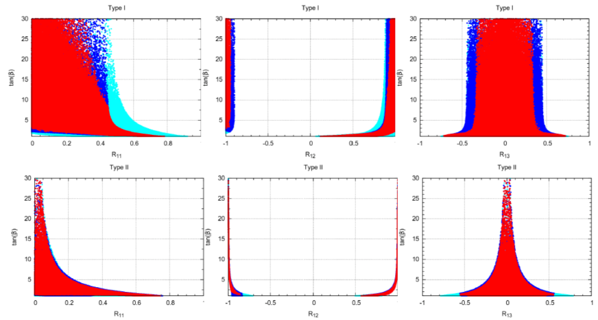
Figure 1: Top: $\tan\beta$ as a function of $R_{11}$ (left), $R_{12}$ (middle) and $R_{13}$ for Type I. Bottom: same but for Type II. The rates are taken to be within 20$\%$ of the SM predictions. The colours are superimposed with cyan/light-grey for $\mu_{VV}$, blue/black for $\mu_{\tau\tau}$ and finally red/dark-grey for $\mu_{\gamma\gamma}$ with $\sqrt{s}=8$ TeV.

The other possibility is to have $R_{11}=c_{1}\,c_{2}=0$ which is still allowed as shown in figure 1 (left). This can be obtained by setting either $c_{2}=0$ or $c_{1}=0$. $c_{2}=0$ is excluded as it would mean $g_{h_{1}VV}=0$, where $V$ is a massive vector boson. Finally we can choose $c_{1}=0$. The values for $a_{F}$ and $b_{F}$ ($F=U,D,L$) in this scenario are presented in Table 2.

Type I		$a_{U}=a_{D}=a_{L}=\tfrac{c_{2}}{s_{\beta}}$		$b_{U}=-b_{D}=-b_{L}=-\tfrac{s_{2}}{t_{\beta}}$
Type II		$a_{D}=a_{L}=0$		$b_{D}=b_{L}=-s_{2}\,t_{\beta}$
Type F		$a_{D}=0$		$b_{D}=-s_{2}\,t_{\beta}$
Type LS		$a_{L}=0$		$b_{L}=-s_{2}\,t_{\beta}$

Table 2: $a_{F}$ and $b_{F}$ limits for $c_{1}=0$ for the four model types.

As shown in table 2 the scenarios where the scalar component vanishes arise only in models Type II, F and LS. In Type II one can have $a_{D}=a_{L}=0$ while in F (LS) only $a_{D}=0$ ($a_{L}=0$) is possible. In this scenario the coupling to gauge bosons is

$$C^{2}=s_{\beta}^{2}c_{2}^{2}\,.$$ (11)

Note that even if $s_{2}=0$ the pseudoscalar component can still be large due to a large value of $\tan\beta$.

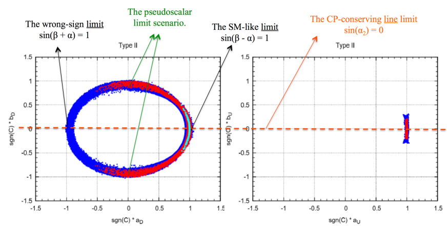
Figure 2: Left: sgn$(C)$ $b_{D}$ $=$ sgn$(C)$ $b_{L}$ as a function of sgn$(C)$ $a_{D}$ $=$ sgn$(C)$ $a_{L}$ for Type II and a center of mass energy of $13$ TeV with all rates at $10$% (blue/black), $5$% (red/dark-grey), and $1$% (cyan/light-grey). Right: same, but for sgn$(C)$ $b_{U}$ as a function of sgn$(C)$ $a_{U}$.

We will now discuss in detail the allowed parameter space in the $(a_{F},b_{F})$ plane for the different model types. We will plot sgn$(C)\,a_{F}$ (sgn$(C)\,b_{F}$) instead of $a_{F}$ ($b_{F}$) with $F=U,D,L$, to avoid the dependence on the phase conventions in choosing the range for the angles $\alpha_{i}$. In the left panel of figure 2 we show $b_{D}=b_{L}$ as a function of $a_{D}=a_{L}$ for Type II and $\sqrt{s}=13$ TeV with all rates at $10$% (blue/black), $5$% (red/dark-grey), and $1$% (cyan/light-grey). We start by noting that this scenario is still possible with the rates within $5$% of the SM value at the LHC and at $\sqrt{s}=13$ TeV. This scenario can only be excluded by a measurement of the rates if the accuracy reaches about $1$%. The constraints on the model force $|b_{D}|\to 1$ when $|a_{D}|\to 0$. When $|b_{D}|\approx 1$, the couplings of the up-type quarks to the lightest Higgs have the form

$$a_{U}^{2}=(1-s_{2}^{4})=(1-1/t_{\beta}^{4}),\quad b_{U}^{2}=s_{2}^{4}=1/t^{4}_{\beta},$$ (12)

while the coupling to massive gauge bosons is now

$$C^{2}=(t^{2}_{\beta}-1)/(t^{2}_{\beta}+1)=(1-s_{2}^{2})/(1+s_{2}^{2})\,.$$ (13)

In the right panel of figure 2 we show $b_{U}$ as a function of $a_{U}$ for Type II with the same colour code. We conclude from the plot that the constraint on the values of $(a_{U},\,b_{U})$ are already quite strong and will be much stronger in the future just taking into account the measurement of the rates.

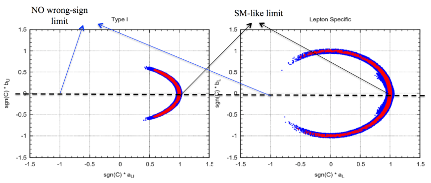
Figure 3: Left: sgn$(C)$ $b_{U}$ as a function of sgn$(C)$ $a_{U}$ for Type I and a center of mass energy of $13$ TeV with all rates at $10$% (blue/black) and $5$% (red/dark-grey). Right: sgn$(C)$ $b_{L}$ as a function of sgn$(C)$ $a_{L}$ for LS and a center of mass energy of $13$ TeV with all rates at $10$% (blue/black) and $5$% (red/dark-grey).

In the left panel of figure 3 we show $b_{U}$ as a function of $a_{U}$ for Type I and $\sqrt{s}=13$ TeV with all rates at $10$% (blue/black) and $5$% (red/dark-grey). We should point out that even at $10$% there are still allowed points close to $(a,b)=(0.5,0.6)$ with no dramatic changes occurring for an increase in accuracy to $5$%. In the right panel we present $b_{L}$ as a function of $a_{L}$ for Type LS with the same colour code. Here again the $(a_{L},b_{L})=(0,1)$ scenario is still allowed with both $10$% and $5$% accuracy. However, as was previously shown, the wrong sign limit is not allowed for the LS model Fontes:2014tga ; Ferreira:2014dya . Nevertheless, in the C2HDM, the scalar component sgn$(C)\,a_{L}$ can reach values close to $-0.8$. Finally, for the up-type and down-type quarks, the plots are very similar to the one in the right panel of figure 2 for Type II.

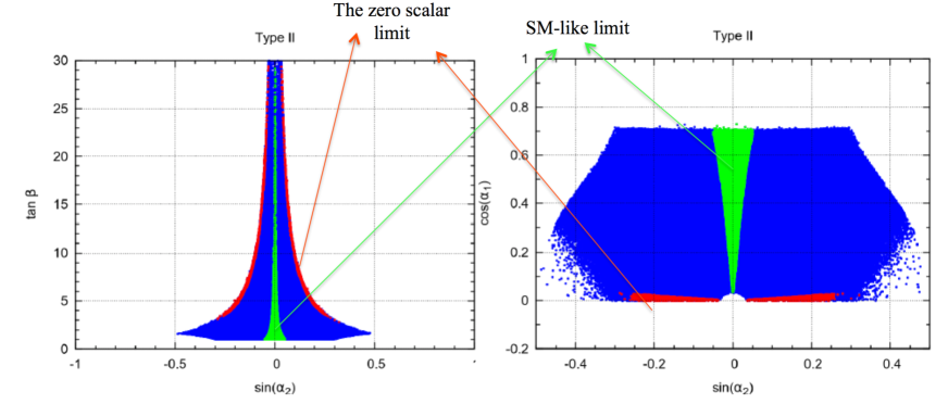
Figure 4: Left: $\tan\beta$ as a function of $\sin\alpha_{2}$ for Type II and a center of mass energy of $13$ TeV with all rates at $10$% (blue/black). In red/dark-grey we show the points with $|a_{D}|<0.1$ and $||b_{D}|-1|<0.1$ and in green $|b_{D}|<0.05$ and $||a_{D}|-1|<0.05$ Right: same, with $\tan\beta$ replaced by $\cos\alpha_{1}$.

In the left panel of figure 4 we present the allowed space in the $\sin\alpha_{2}$-$\tan{\beta}$ plane, for Type II and $\sqrt{s}=13$ TeV. Rates at $10$% are shown in blue/black while in red/dark-grey we present the points with $|a_{D}|<0.1$ and $||b_{D}|-1|<0.1$ and in green $|b_{D}|<0.05$ and $||a_{D}|-1|<0.05$. The right panel now shows the allowed space in the $\sin\alpha_{2}$-$\cos\alpha_{1}$ plane. The purpose of these plots is to pinpoint the main differences between the SM-like scenario, where $(|a_{D}|,|b_{D}|)\approx(1,0)$ and the pseudoscalar scenario where $(|a_{D}|,|b_{D}|)\approx(0,1)$. In the SM-like scenario $\sin\alpha_{2}\approx 0$, $\tan\beta$ is not constrained and the allowed values of $\sin\alpha_{2}$ grow with increasing $\cos\alpha_{1}$. In the pseudoscalar scenario $\cos\alpha_{1}\approx 0$, $\sin\alpha_{2}$ and $\tan\beta$ are strongly correlated and $\tan\beta$ has to be above $\approx 3$. We note that all values of $a_{D}$ and $b_{D}$ are allowed provided $a_{D}^{2}+b_{D}^{2}\approx 1$.

III.1 Direct measurements of the CP-violating angle

We have seen that the precise measurements of the Higgs couplings allows us to constrain both the scalar and the pseudoscalar Yukawas in the C2HDM. However, a direct measurement of the relative size of the pseudoscalar to scalar coupling is important because it directly probes the Higgs couplings to light quarks and leptons. Moreover, when combined with EDMs it can provide universality tests for the CP-odd components of the Yukawas.

The angle that measures the pseudoscalar to scalar ratio, $\phi_{i}$, is defined by

$$\tan\phi_{i}=b_{i}/a_{i}\qquad i=U,\,D,\,L\,,$$ (14)

and could in principle be measured for all Yukawa couplings. Direct measurements of this ratio in the up-quark sector, $b_{U}/a_{U}$, was first proposed in Gunion:1996xu and more recently in Ellis:2013yxa ; He:2014xla ; Boudjema:2015nda . The process $pp\to hjj$ DelDuca:2001fn also allows to probe the same vertex as discussed in Field:2002gt ; Dolan:2014upa . In reference Dolan:2014upa an exclusion of $\phi_{t}>40\degree$ ($\phi_{t}>25\degree$) for a luminosity of 50 fb^-1 (300 fb^-1) was obtained for 14 TeV and assuming $\phi_{t}=0$ as the null hypothesis. A study of the $\tau^{+}\tau^{-}h$ vertex was proposed in Berge:2008wi (see also Harnik:2013aja ; Askew:2015mda ) and a detailed study taking into account the main backgrounds Berge:2014sra lead to an estimate in the precision of $\Delta\phi_{\tau}$ of $27\degree$ ($14.3\degree$) for a luminosity of 150 fb^-1 (500 fb^-1) and $\sqrt{s}=14$ Tev.

The number of independent measurements of $\phi_{i}$ one needs depends on the C2HDM Yukawa type. For Type I one process is enough since $\phi_{U}=\phi_{D}=\phi_{L}$. For all other types we need two independent measurements. For type II and LS the planned measurements of $\phi_{t}$ and $\phi_{\tau}$ would be enough while for type F we would need $\phi_{b}$. Incompatibility in the measured values of $\phi_{t}$ and $\phi_{\tau}$ would exclude both Type I and F.

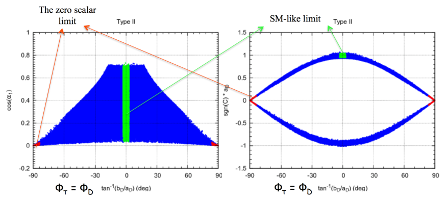
Figure 5: Left: $\cos\alpha_{1}$ as a function of $\tan^{-1}(b_{D}/a_{D})$ for Type II and a center of mass energy of $13$ TeV with all rates at $10$% (blue/black). In red/dark-grey we show the points with $|a_{D}|<0.1$ and $||b_{D}|-1|<0.1$ and in green $|b_{D}|<0.05$ and $||a_{D}|-1|<0.05$. Right: same, with $\cos\alpha_{1}$ replaced by sgn$(C)\,a_{D}$.

We will now discuss the behaviour of $\cos\alpha_{1}$ (figure 5 left) and sgn$(C)\,a_{D}$ (figure 5 right) as a function of $\phi_{D}=\phi_{\tau}$ for Type II. In figure 5 $\sqrt{s}=13$ TeV and all rates are taken at $10$% (blue/black); in red/dark-grey we show the points with $|a_{D}|<0.1$ and $||b_{D}|-1|<0.1$ and in green $|b_{D}|<0.05$ and $||a_{D}|-1|<0.05$. The SM-like scenario sgn$(C)$ $(a_{D},\,b_{D})=(1,0)$ is easily distinguishable from the $(0,1)$ scenario. In fact, a measurement of $\phi_{\tau}$ even if not very precise would easily exclude one of the scenarios. Obviously, all other scenarios in between these two will need more precision (and other measurements) to find the values of scalar and pseudoscalar components. The $\tau^{+}\tau^{-}h$ angle is related to $\alpha_{2}$ as

$$\tan\phi_{\tau}=-s_{\beta}/c_{1}\,\tan\alpha_{2}\qquad\Rightarrow\qquad\tan\alpha_{2}=-c_{1}/s_{\beta}\,\tan\phi_{\tau}$$ (15)

and therefore a measurement of the angle $\phi_{\tau}$ does not directly constrain the angle $\alpha_{2}$ but rather a relation between the three angles. A measurement of $\phi_{t}$ and $\phi_{\tau}$ would give us two independent relations to determine the three angles.

III.2 Constraints from EDM

The C2HDM, as all models with CP violation, are constrained by bounds arising from the measurement of electric dipole moments (EDMs) of neutrons, atoms and molecules. The parameter space of the C2HDM was analysed in Buras:2010zm ; Cline:2011mm ; Jung:2013hka ; Shu:2013uua ; Inoue:2014nva ; Brod:2013cka and ref. Inoue:2014nva found that the most stringent bounds are obtained using the results from the ACME Collaboration Baron:2013eja , except when cancellations among the neutral scalars occur. These cancellations were pointed out in Jung:2013hka ; Shu:2013uua and arise due to orthogonality of the $R$ matrix in the case of almost degenerate scalars Fontes:2014xva .

The scenarios we discuss have the couplings of the up-type sector (top quark) very close to the SM ones. Indeed, only the couplings in the down-type sector, namely tau lepton and the b-quark Yukawa couplings, are still allowed by data to have a vanishing scalar component. Due to the universality of the lepton Yukawa couplings the electron EDM also restricts the tau Yukawa. In a type II model this in turn also restricts the b-quark Yukawa of the SM-like Higgs. However, this is completely irrelevant in the Flipped model, where the charged leptons couple as the up-type quarks. We have shown in Fontes:2015mea that in a preliminary scan over the parameter space we have found points which pass all constraints including ACME’s.

A dedicated study of the EDM contributions in the Type II C2HDM, where there are several sources of CP violation and where the partial cancellations of the various scalars is dully taken into account is in progress us_edm . In addition, one should keep in mind that, as pointed out in ref. Brod:2013cka ; Dekens:2014jka , the future bounds from the EDMs can have a strong impact on the C2HDM. In the future, the interplay between the EDM bounds and the data from the LHC Run 2 will pose relevant new constraints in the complex 2HDM in general, and in particular for the scenarios presented in this work.

IV Conclusions

We have discussed the interesting possibility of having a vanishing scalar component is some of the Yukawa couplings, namely the couplings of the lightest Higgs to down-type quarks and/or to leptons. These scenarios can occur for Type II, F and LS, and the pseudoscalar component plays the role of the scalar component in assuring the measured rates at the LHC. A direct measurement of the angles that gauge the ratio of pseudoscalar to scalar components is needed to further constrain the model. In particular, the measurement of $\phi_{\tau}$, the angle for the $\tau^{+}\tau^{-}h$ vertex, will allow to either confirm or to rule out the scenario of a vanishing scalar, even with a poor accuracy. We have also noted that for the Type F, only a direct measurement of $\phi_{D}$ in a process involving the $bbh$ vertex would probe the vanishing scalar scenario. Finally a future linear collider Ono:2012ah ; Asner:2013psa will certainly help to further probe the vanishing scalar scenarios.

- (1) G. Aad et al. [ATLAS Collaboration], Phys. Lett. B 716, 1 (2012) [arXiv:1207.7214 [hep-ex]].
- (2) S. Chatrchyan et al. [CMS Collaboration], Phys. Lett. B 716, 30 (2012) [arXiv:1207.7235 [hep-ex]].
- (3) T.D. Lee, Phys. Rev. D 8 (1973) 1226.
- (4) J.F. Gunion, H.E. Haber, G.L. Kane and S. Dawson, The Higgs Hunter’s Guide (Westview Press, Boulder, CO, 2000).
- (5) G. C. Branco, P. M. Ferreira, L. Lavoura, M. N. Rebelo, M. Sher, and J. P. Silva, Theory and phenomenology of two-Higgs-doublet models, Phys. Rept. 516 (2012) 1 [arXiv:1106.0034 [hep-ph]].
- (6) A. Barroso, P. M. Ferreira, R. Santos and J. P. Silva, Phys. Rev. D 86 (2012) 015022 [arXiv:1205.4247 [hep-ph]].
- (7) S. Inoue, M. J. Ramsey-Musolf and Y. Zhang, Phys. Rev. D 89 (2014) 115023 [arXiv:1403.4257 [hep-ph]].
- (8) K. Cheung, J. S. Lee, E. Senaha and P. Y. Tseng, JHEP 1406 (2014) 149 [arXiv:1403.4775 [hep-ph]].
- (9) D. Fontes, J. C. Romão and J. P. Silva, JHEP 1412, 043 (2014) [arXiv:1408.2534 [hep-ph]].
- (10) J. Brod, U. Haisch and J. Zupan, JHEP 1311 (2013) 180 [arXiv:1310.1385 [hep-ph], arXiv:1310.1385].
- (11) ATLAS Collaboration, Physics at a High-Luminosity LHC with ATLAS, (2013), arXiv:1307.7292 [hep-ex], SNOW13-00078; ATLAS Collaboration, Projections for measurements of Higgs boson cross sections, branching ratios and coupling parameters with the ATLAS detector at a HL-LHC, ATLAS-PHYS-PUB-2013-014 (2013).
- (12) CMS Collaboration, Projected Performance of an Upgraded CMS Detector at the LHC and HL-LHC: Contribution to the Snowmass Process, (2013), arXiv:1307.7135 [hep-ex], SNOW13-00086.
- (13) S. Dawson, A. Gritsan, H. Logan, J. Qian, C. Tully, R. Van Kooten, A. Ajaib and A. Anastassov et al., arXiv:1310.8361 [hep-ex].
- (14) D. Fontes, J. C. Romão, R. Santos and J. P. Silva, JHEP, to be published, arXiv:1502.01720 [hep-ph].
- (15) I. F. Ginzburg, M. Krawczyk and P. Osland, Two Higgs doublet models with CP violation, hep-ph/0211371.
- (16) W. Khater and P. Osland, CP violation in top quark production at the LHC and two Higgs doublet models, Nucl. Phys. B 661 (2003) 209 [hep-ph/0302004].
- (17) A. W. El Kaffas, P. Osland and O. M. Ogreid, CP violation, stability and unitarity of the two Higgs doublet model, Nonlin. Phenom. Complex Syst. 10(2007) 347 [hep-ph/0702097].
- (18) A. W. El Kaffas, W. Khater, O. M. Ogreid, and P. Osland, Consistency of the two Higgs doublet model and CP violation in top production at the LHC, Nucl. Phys. B 775 (2007) 45 [hep-ph/0605142].
- (19) B. Grzadkowski and P. Osland, Tempered Two-Higgs-Doublet Model, Phys. Rev. D 82 (2010) 125026 [arXiv:0910.4068 [hep-ph]].
- (20) A. Arhrib, E. Christova, H. Eberl and E. Ginina, CP violation in charged Higgs production and decays in the Complex Two Higgs Doublet Model, JHEP 1104 (2011) 089 [arXiv:1011.6560 [hep-ph]].
- (21) L. Lavoura, J. P. Silva, Fundamental CP violating quantities in a model with many Higgs doublets, Phys. Rev. D 50 (1994) 4619 [hep-ph/9404276].
- (22) F. J. Botella and J. P. Silva, Jarlskog - like invariants for theories with scalars and fermions, Phys. Rev. D 51 (1995) 3870 [hep-ph/9411288].
- (23) S.L. Glashow and S. Weinberg, Phys. Rev. D 15, 1958 (1977); E.A. Paschos, Phys. Rev. D 15, 1966 (1977).
- (24) G. Aad et al. [ATLAS Collaboration], Phys. Rev. D 90 (2014) 5, 052004 [arXiv:1406.3827 [hep-ex]].
- (25) V. Khachatryan et al. [CMS Collaboration], arXiv:1412.8662 [hep-ex].
- (26) T. Hermann, M. Misiak and M. Steinhauser, JHEP 1211 (2012) 036 [arXiv:1208.2788 [hep-ph]]; F. Mahmoudi and O. Stal, Phys. Rev. D 81, 035016 (2010) [arXiv:0907.1791 [hep-ph]].
- (27) O. Deschamps, S. Descotes-Genon, S. Monteil, V. Niess, S. T’Jampens and V. Tisserand, Phys. Rev. D 82, 073012 (2010) [arXiv:0907.5135 [hep-ph]].
- (28) M. Baak, M. Goebel, J. Haller, A. Hoecker, D. Ludwig, K. Moenig, M. Schott and J. Stelzer, Updated Status of the Global Electroweak Fit and Constraints on New Physics, Eur. Phys. J. C 72 (2012) 2003 [arXiv:1107.0975 [hep-ph]]
- (29) A. Denner, R.J. Guth, W. Hollik and J.H. Kuhn, Z. Phys. C 51, 695 (1991); H.E. Haber and H.E. Logan, Phys. Rev. D 62, 015011 (2000) [hep-ph/9909335]; A. Freitas and Y.-C. Huang, JHEP 1208, 050 (2012) [arXiv:1205.0299 [hep-ph]].
- (30) G. Abbiendi et al. [ALEPH and DELPHI and L3 and OPAL and LEP Collaborations], Eur. Phys. J. C 73 (2013) 2463 [arXiv:1301.6065 [hep-ex]].
- (31) ATLAS collaboration, ATLAS-CONF-2013-090; G. Aad et al. [ATLAS Collaboration], JHEP 1206 (2012) 039 [arXiv:1204.2760 [hep-ex]]; G. Aad et al. [ATLAS Collaboration], arXiv:1412.6663 [hep-ex].
- (32) S. Chatrchyan et al. [CMS Collaboration], JHEP 1207 (2012) 143 [arXiv:1205.5736 [hep-ex]]; CMS Note, CMS-PAS-HIG-14-020.
- (33) The ALEPH, CDF, D0, DELPHI, L3, OPAL, SLD Collaborations, the LEP Electroweak Working Group, the Tevatron Electroweak Working Group, and the SLD electroweak and heavy flavour Groups, arXiv:1012.2367 [hep-ex].
- (34) G. Aad et al. [ATLAS Collaboration], Phys. Lett. B 710 (2012) 383 [arXiv:1202.1415 [hep-ex]].
- (35) S. Chatrchyan et al. [CMS Collaboration], Eur. Phys. J. C 73 (2013) 2469 [arXiv:1304.0213 [hep-ex]].
- (36) G. Aad et al. [ATLAS Collaboration], JHEP 1411 (2014) 056 [arXiv:1409.6064 [hep-ex]].
- (37) V. Khachatryan et al. [CMS Collaboration], Phys. Rev. D 90 (2014) 112013 [arXiv:1410.2751 [hep-ex]].
- (38) N. G. Deshpande and E. Ma, Pattern of Symmetry Breaking with Two Higgs Doublets, Phys. Rev. D 18 (1978) 2574 .
- (39) S. Kanemura, T. Kubota and E. Takasugi, Lee-Quigg-Thacker bounds for Higgs boson masses in a two doublet model, Phys. Lett. B 313 (1993) 155 [hep-ph/9303263].
- (40) A. G. Akeroyd, A. Arhrib and E. -M. Naimi, Note on tree level unitarity in the general two Higgs doublet model, Phys. Lett. B 490(2000) 119 [hep-ph/0006035].
- (41) I. F. Ginzburg and I. P. Ivanov, Tree level unitarity constraints in the 2HDM with CP violation, hep-ph/0312374.
- (42) M.E. Peskin and T. Takeuchi, Phys. Rev. D 46, 381 (1992).
- (43) W. Grimus, L. Lavoura, O. M. Ogreid and P. Osland, The Oblique parameters in multi-Higgs-doublet models Nucl. Phys. B 801 (2008) 81 [arXiv:0802.4353 [hep-ph]].
- (44) M. Baak, M. Goebel, J. Haller, A. Hoecker, D. Kennedy, R. Kogler, K. Moenig and M. Schott et al., The Electroweak Fit of the Standard Model after the Discovery of a New Boson at the LHC, Eur. Phys. J. C 72 (2012) 2205 [arXiv:1209.2716 [hep-ph]].
- (45) M. Spira, HIGLU: A program for the calculation of the total Higgs production cross-section at hadron colliders via gluon fusion including QCD corrections, hep-ph/9510347.
- (46) R. V. Harlander, S. Liebler and H. Mantler, SusHi: A program for the calculation of Higgs production in gluon fusion and bottom-quark annihilation in the Standard Model and the MSSM, Comput. Phys. Commun. 184 (2013) 1605 [arXiv:1212.3249 [hep-ph]].
- (47) https://twiki.cern.ch/twiki/bin/view/LHCPhysics/CrossSectionsFigures .
- (48) D. Fontes, J. C. Romão and J. P. Silva, Phys. Rev. D 90, no. 1, 015021 (2014) [arXiv:1406.6080 [hep-ph]].
- (49) P. M. Ferreira, R. Guedes, M. O. P. Sampaio and R. Santos, JHEP 1412 (2014) 067 [arXiv:1409.6723 [hep-ph]].
- (50) J. F. Gunion and X. G. He, Phys. Rev. Lett. 76 (1996) 4468 [hep-ph/9602226].
- (51) J. Ellis, D. S. Hwang, K. Sakurai and M. Takeuchi, JHEP 1404 (2014) 004 [arXiv:1312.5736 [hep-ph]].
- (52) X. G. He, G. N. Li and Y. J. Zheng, arXiv:1501.00012 [hep-ph].
- (53) F. Boudjema, R. M. Godbole, D. Guadagnoli and K. A. Mohan, arXiv:1501.03157 [hep-ph].
- (54) V. Del Duca, W. Kilgore, C. Oleari, C. Schmidt and D. Zeppenfeld, Nucl. Phys. B 616 (2001) 367 [hep-ph/0108030].
- (55) B. Field, Phys. Rev. D 66 (2002) 114007 [hep-ph/0208262].
- (56) M. J. Dolan, P. Harris, M. Jankowiak and M. Spannowsky, Phys. Rev. D 90 (2014) 7, 073008 [arXiv:1406.3322 [hep-ph]].
- (57) S. Berge, W. Bernreuther and J. Ziethe, Phys. Rev. Lett. 100 (2008) 171605 [arXiv:0801.2297 [hep-ph]].
- (58) R. Harnik, A. Martin, T. Okui, R. Primulando and F. Yu, Phys. Rev. D 88 (2013) 7, 076009 [arXiv:1308.1094 [hep-ph]].
- (59) A. Askew, P. Jaiswal, T. Okui, H. B. Prosper and N. Sato, arXiv:1501.03156 [hep-ph].
- (60) S. Berge, W. Bernreuther and S. Kirchner, Eur. Phys. J. C 74 (2014) 11, 3164 [arXiv:1408.0798 [hep-ph]].
- (61) A. J. Buras, G. Isidori and P. Paradisi, Phys. Lett. B 694, 402 (2011) [arXiv:1007.5291 [hep-ph]].
- (62) J. M. Cline, K. Kainulainen and M. Trott, JHEP 1111, 089 (2011) [arXiv:1107.3559 [hep-ph]].
- (63) M. Jung and A. Pich, JHEP 1404, 076 (2014) [arXiv:1308.6283 [hep-ph]].
- (64) J. Shu and Y. Zhang, Phys. Rev. Lett. 111, no. 9, 091801 (2013) [arXiv:1304.0773 [hep-ph]].
- (65) J. Baron et al. [ACME Collaboration], Science 343, 269 (2014) [arXiv:1310.7534 [physics.atom-ph]].
- (66) D. Fontes, J. C. Romão, R. Santos and J. P. Silva, to appear.
- (67) W. Dekens, J. de Vries, J. Bsaisou, W. Bernreuther, C. Hanhart, U. G. Meißner, A. Nogga and A. Wirzba, JHEP 1407 (2014) 069 [arXiv:1404.6082 [hep-ph]].
- (68) H. Ono and A. Miyamoto, Eur. Phys. J. C 73 (2013) 2343.
- (69) D.M. Asner, T. Barklow, C. Calancha, K. Fujii, N. Graf, H.E. Haber, A. Ishikawa, S. Kanemura et al., arXiv:1310.0763 [hep-ph].