Work distribution function for a Brownian particle driven by a nonconservative force

Abstract

We derive the distribution function of work performed by a harmonic force acting on a uniformly dragged Brownian particle subjected to a rotational torque. Following the Onsager and Machlup’s functional integral approach, we obtain the transition probability of finding the Brownian particle at a particular position at time $t$ given that it started the journey from a specific location at an earlier time. The difference between the forward and the time-reversed form of the generalized Onsager-Machlup’s Lagrangian is identified as the rate of medium entropy production which further helps us develop the stochastic thermodynamics formalism for our model. The probability distribution for the work done by the harmonic trap is evaluated for an equilibrium initial condition. Although this distribution has a Gaussian form, it is found that the distribution does not satisfy the conventional work fluctuation theorem.

1 Introduction

Fluctuations are ubiquitous in most of the physical processes we observe in nature. In general, though the effect of fluctuations could be ignored for the coarse grained description of the average thermodynamic quantities, these are no longer negligible for small systems, like, biomolecules, nano-machines etc. For instance, the movement of a molecular motor of nanometer size is affected significantly by the mean thermal energy of the surrounding medium which causes the motor’s position to fluctuate. In linear irreversible processes, these fluctuations obey a general principle known as the fluctuation-dissipation theorem kubo ; kubo_book . However, in the case of systems far away from equilibrium, the assumptions of the linear-response theory are not valid since the fluctuations of the thermodynamic variables do not follow the linear law of relaxation.

Since the finding of the fluctuation relations for the probabilities of observing the entropy producing and consuming trajectories in simulations of shearing fluid nearly two decades ago evans1 , there has been a vast number of studies evans2 ; gallavotti ; kurchan ; jarzynskirel ; crooks ; lebowitz ; zon ; zon_cohen1 ; zon_cohen2 ; harris ; seifert2 ; seifert ; seifert1 ; esposito ; noneql_book ; derrida extending the ideas and formalisms of linear irreversible thermodynamics to nonequilibrium systems. The emphasis of the fluctuation relations has been on quantifying the asymmetry between the probability distributions of a time-integrated quantity $\Sigma_{t}$ to have values $\pm W$ in the forward and time-reversed processes, and it is expressed in the mathematical form as $\frac{P_{F}(\Sigma_{t}=+W)}{P_{R}(\Sigma_{t}^{\dagger}=-W)}=\exp(W/k_{B}T)$. $\Sigma_{t}$ could represent the work done by an external force, dissipated heat, entropy production etc, and $\Sigma_{t}^{\dagger}$ stands for the same thermodynamic quantity in the time-reversed process. These relations, valid for systems far-from-equilibrium, could be reduced to the fluctuation-dissipation theorem for near-equilibrium processes derrida . Of the many ramifications of the fluctuation relations, the most notable results are the Jarzynski equality jarzynskirel and Crooks work relation crooks which relate the asymmetry to the free energy difference between the initial and final equilibrium states which are connected through a reversible or irreversible transformation. Although, to prove the fluctuation relations, one does not always require to obtain the detailed distribution functions, to verify them experimentally, however, it is preferable to get the histograms of the relevant thermodynamic quantities. In many situations ritort , a detailed knowledge of the distribution of the nonequilibrium work might be essential to compute the equilibrium free energy difference utilizing the Jarzynski equality. Despite the significant progress in the theoretical studies of these distribution functions for work, heat, entropy production etc for a variety of nonequilibrium systems zon ; zon_cohen1 ; zon_cohen2 ; mazonka ; seifert3 ; imparato3 ; farago ; ritort ; imparato1 ; park1 ; park2 ; sanjib1 ; sanjib2 (and the references therein), the derivation of the exact analytical expressions for these distributions are not so many. This is possibly due to the increasing difficulty in obtaining the analytical solutions in closed forms as the dynamics of the system becomes more complex.

In this paper, we derive the positional probability distribution and the work distribution function for a Brownian particle using the Onsager-Machlup’s functional integral approach. In their theory of linear relaxation processes, Onsager and Machlup developed a path integral approach onsager1 ; onsager2 for the probability distribution functions of trajectories in the configuration space with specific initial and final states. Using a variational technique they subsequently showed that this approach leads to Onsager’s minimal energy dissipation. Recently, there have been many efforts to generalize the Onsager-Machlup theory for systems in nonequilibrium steady states bertini1 ; bertini2 ; bertini3 ; imparato2 ; taniguchi ; cohen ; maes ; jstat2 . Extending this approach, Taniguchi and Cohen taniguchi ; cohen obtained the distribution functions of work, dissipated heat for a uniformly dragged Brownian particle. Further, after expressing the Onsager-Machlup Lagrangian in terms of the dissipation functions and the entropy production rate, they showed how these fluctuating quantities satisfy the energy conservation law and the second law of thermodynamics. Similar variational scheme has also been considered to obtain the probability distributions of thermodynamic quantities for a variety of systems engel .

In the present work, we consider two dimensional motion of a Brownian particle which is subjected to a nonconservative force and a confining harmonic potential with its minimum moving with a uniform velocity $v$. The nonconservative force

$$f=-yn\hat{x}+xn\hat{y},$$ (1)

with $n$ denoting the strength of the force, produces an anticlockwise drift about the origin. The nonconservative force can arise due to a vortex centered at the origin of the system in the surrounding liquid vladimir . Both the time dependent confining potential and the nonconservative force are responsible for breaking the detailed balance and driving the system out of equilibrium. For this model, we derive the joint probability distribution which gives the probability of finding a Brownian particle at a given position at a specific time. After defining the forward and the time-reversed trajectories, we obtain the expression for the dissipated heat and the energy conservation relation. In the process, we identify various works, namely, the work done by the harmonic trap which can be identified as the thermodynamic work jarzynskirel and the mechanical work done by the nonconservative force park1 ; park2 . Finally, using a variational approach, we obtain the distribution function for the work done by the trap. The work distribution has a Gaussian form with the mean and the variance having a nontrivial oscillatory dependence originating from the nonconservative force. Although, this distribution is Gaussian, it does not satisfy the conventional fluctuation relation. Physically, the presence of the nonconservative force makes the role of the thermal fluctuation negligible. Similar deviation can also be found in ciliberto2 ; joubaud for the motion of a torsion pendulum driven by an external time dependent torque.

The rest of the paper is organized in the following way. In section 2, we introduce two coupled Langevin equations describing the motion of the Brownian particle in the $x-y$ plane. In section 3, we find out the joint probability distribution for the position of the Brownian particle. Starting with the Fokker-Planck equation for the joint probability distribution, we express first the transition probability in a functional integral form and subsequently evaluate the path integrals employing Onsager-Machlup’s variational approach. The joint probability distribution is obtained from the expression of the transition probability. From the generalized Onsager-Machlup Lagrangian, we define in section 4 the thermodynamic work, mechanical work, dissipated heat and the entropy production of the medium. We further show here the validity of the energy conservation relation and the second law of thermodynamics for a trajectory. In section 5, we obtain the explicit form of the distribution function of the thermodynamic work. We summarize our findings and discuss possible future research on this model in section 6. Some of the details of the derivations and algebra are presented in the appendices.

2 The model

The Brownian particle considered here moves in a plane under the influence of the potential $U[x(t),y(t),t]=\frac{k}{2}\left\{(x(t)-vt)^{2}+y(t)^{2}\right\}$ and a nonconservative force as given in equation (1) vladimir ; park2 . Here $v$ is the constant velocity with which the harmonic trap moves along the $x$ direction.

The overdamped Langevin equations describing the motion of the particle in the $x$-$y$ plane are expressed as

$$\dot{x} = -\frac{1}{\tau_{r}}(x-vt)-\sigma y+\frac{1}{\alpha}\xi_{x}(t),$$ (2)

$$\dot{y} = -\frac{1}{\tau_{r}}y+\sigma x+\frac{1}{\alpha}\xi_{y}(t),$$ (3)

where, $\alpha$ is the viscous drag coefficient, $\sigma=n/\alpha$ and $\tau_{r}=\alpha/k$ is the relaxation time of the trap. The overdots imply derivatives with respect to time, $t$. $\xi_{x}(t)$ and $\xi_{y}(t)$ represent the Gaussian-distributed thermal noise having zero mean and correlations as

$$\left\langle\xi_{i}(t)\xi_{j}(t^{\prime})\right\rangle=\frac{2\alpha}{\beta}\ \delta_{ij}\delta(t-t^{\prime}).$$ (4)

Here $\beta=(k_{B}T)^{-1}$ and $i,\ j$ correspond to the $x,\ y$ coordinates.

3 Probability distribution functions related to the location of the particle

The joint probability distribution is defined as the probability of finding the Brownian particle at position $(x,y)$ at time $t$. The time evolution of the joint probability distribution is governed by the Fokker-Planck equation which can be written as

$$\frac{\partial\rho(x,y,t)}{\partial t}=\hat{L}_{\rm FP}\ \rho(x,y,t),$$ (5)

where, the Fokker-Planck operator $\hat{L}_{\rm FP}$ is given by,

$$\hat{L}_{\rm FP} = \frac{\partial}{\partial x}\left\{(x-vt)/\tau_{r}+\sigma y\right\}-\frac{\partial}{\partial y}\left\{-y/\tau_{r}+\sigma x\right\}$$ (6)

$$+D\frac{\partial^{2}}{\partial x^{2}}+D\frac{\partial^{2}}{\partial y^{2}},$$

with the diffusion constant, $D=1/(\alpha\beta)$. Let us consider the simplest situation where $v=\sigma=0$. Writing the Fokker-Planck equation in terms of the probability current, ${\bf J}_{\rho}$, we have

$$\frac{\partial\rho}{\partial t}=-\nabla\cdot{\bf J}_{\rho},$$ (7)

where

$${\bf J}_{\rho}={\hat{x}}\left[\frac{x\rho}{\tau_{r}}+\frac{D\partial\rho}{\partial x}\right]+{\hat{y}}\left[\frac{y\rho}{\tau_{r}}+\frac{D\partial\rho}{\partial y}\right].$$ (8)

Substituting $\rho=\exp[-\beta U]$ (with $v=0$), we obtain a vanishing stationary current corresponding to the equilibrium situation of a fixed harmonic potential. This is the situation where the detailed balance is satisfied. The nonconservative force which cannot be expressed in the form of a gradient of a potential violates the detailed balance.

$\rho(x,y,t)$ can be expressed in terms of the transition probability $P(x,y,t\mid x_{0},y_{0},t_{0})$ which gives the probability of finding a Brownian particle at position $(x,y)$ at time $t$, given that it was at $(x_{0},y_{0})$ at an initial time $t_{0}$. For simplicity, we choose $t_{0}=0$ and denote the transition probability as $P(x,y,t\mid x_{0},y_{0})$. The Fokker-Planck equation (5) allows us to obtain the following path integral representation for the transition probability risken (some of the details of the derivation are presented in appendix-A)

$$P(x_{f},y_{f},t_{f}\mid x_{0},y_{0})= \int{\cal D}[x(t)]\ \int{\cal D}[y(t)]$$

$$\times\exp\left(-\int_{0}^{t_{f}}{\cal L}(x,y,\dot{x},\dot{y},t)\,\textrm{d}t\right).$$ (9)

${\cal L}(x,y,\dot{x},\dot{y},t)$ is the generalized Onsager-Machlup Lagrangian having the form

$${\cal L}(x,y,\dot{x},\dot{y},t) = \frac{1}{4D}\bigl{[}(\dot{x}+(x-vt)/\tau_{r}+\sigma y)^{2}$$ (10)

$$+(\dot{y}+y/\tau_{r}-\sigma x)^{2}\bigr{]}.$$

We evaluate the functional integrals (9) using a variational approach onsager1 ; onsager2 ; wiegel ; taniguchi ; cohen , in which one evaluates the most probable path that gives the most significant contribution to the functional integral. This is expected to be a good approximation for low noise strength or $D\rightarrow 0$ wiegel . The approximate form of the transition probability can be written as

$$P(x_{f},y_{f},t_{f}\mid x_{0},y_{0})\propto\exp\Bigl{(}-\Bigl{[}\int_{0}^{t_{f}}{\cal L}(x,y,\dot{x},\dot{y},t)\,\textrm{d}t\Bigr{]}_{\rm min}\Bigr{)},$$ (11)

where the object in the square bracket is evaluated over the most probable path leading to the largest value of the exponential. The most-probable path is determined by using the extremization condition

$$\delta\int_{0}^{t_{f}}{\cal L}(x,y,\dot{x},\dot{y},t)\,\textrm{d}t=0.$$ (12)

Doing a Taylor-expansion around the optimal values, $(x_{c},y_{c})$, and retaining fluctuations about the optimal path, $u=(x-x_{c})$ and $z=(y-y_{c})$ up to second order the transition probability in (9) can be written as,

$$P(x_{f},y_{f},t_{f}\mid x_{0},y_{0}) =\phi(t_{f})$$

$$\times\exp\left(-\int_{0}^{t_{f}}{\cal L}(x_{c},y_{c},\dot{x}_{c},\dot{y}_{c},t)\,\textrm{d}t\right).$$ (13)

Since we consider trajectories with fixed end-points and allow no variation at the end points, $u$ and $z$ satisfy Dirichlet boundary conditions $u(0)=0,\ u(t_{f})=0,\ z(0)=0,\ z(t_{f})=0$. As a consequence of this, the fluctuation factor

$$\phi(t_{f})=\int_{u(0)=0}^{u(t_{f})=0}{\cal D}[u(t)]\,\int_{z(0)=0}^{z(t_{f})=0}{\cal D}[z(t)]$$

$$\times\exp\biggl{\{}-\frac{1}{4D}\left(\left[\dot{u}+u/\tau_{r}+\sigma z\right]^{2}+\left[\dot{z}+z/\tau_{r}-\sigma u\right]^{2}\right)\biggr{\}},$$ (14)

is a function of the final time $t_{f}$ only. Instead of evaluating the path integrals in Eq. (14) directly, we determine $\phi(t_{f})$ using the normalization condition of the transition probability, i.e., the total probability of finding the Brownian particle at any final value of $(x_{f},y_{f})$ after time $t_{f}$ is unity. It can be proved, a posteriori, from the normalization property of $P(x_{f},y_{f},t_{f}\mid x_{0},y_{0})\mid_{v=0}$, that the final expression of $\phi(t_{f})$ has the form

$$\phi(t_{f})=\frac{\left[1+\coth(t_{f}/\tau_{r})\right]}{4\pi D\tau_{r}}.$$ (15)

The extremization condition (12) leads to two coupled Euler-Lagrange equations for the optimal paths $x_{c}(t)$ and $y_{c}(t)$

$$\ddot{x}_{c}-(\sigma^{2}+1/\tau_{r}^{2})x_{c}+2\sigma\dot{y}_{c}+v\left(\frac{t}{\tau_{r}^{2}}-\frac{1}{\tau_{r}}\right)=0$$ (16)

$$\ddot{y}_{c}-(\sigma^{2}+1/\tau_{r}^{2})y_{c}-2\sigma\dot{x}_{c}+v\sigma t/\tau_{r}=0.$$ (17)

The solutions of the above equations are

$$x_{c}(t) = v[bt-\tau_{r}+\sigma^{2}\tau_{r}^{3}]/b^{2}$$ (18)

$$+\cosh(t/\tau_{r})[a_{2}\cos(\sigma t)-a_{1}\sin(\sigma t)]$$

$$+\sinh(t/\tau_{r})[a_{4}\cos(\sigma t)-a_{3}\sin(\sigma t)],$$

$$y_{c}(t) = \sigma\tau_{r}v[bt-2\tau_{r}]/b^{2}$$ (19)

$$+\cosh(t/\tau_{r})[a_{1}\cos(\sigma t)+a_{2}\sin(\sigma t)]$$

$$+\sinh(t/\tau_{r})[a_{3}\cos(\sigma t)+a_{4}\sin(\sigma t)],$$

where $b=(1+\sigma^{2}\tau_{r}^{2})$. The constants $a_{1},\ a_{2},\ a_{3}$ and $a_{4}$ are calculated using the boundary conditions $x_{c}(0)=\nobreak x_{0},\ x_{c}(t_{f})=x_{f},\ y_{c}(0)=y_{0},\ y_{c}(t_{f})=y_{f}$. These constants are

$$a_{1} = y_{0}+2\sigma v\tau_{r}^{2}/b^{2},$$ (20)

$$a_{2} = x_{0}-v(\sigma^{2}\tau_{r}^{3}-\tau_{r})/b^{2},$$ (21)

$$a_{3} = -\frac{{\rm csch}(t_{f}/\tau_{r})}{b^{2}}\biggl{\{}\cos(\sigma t_{f})\left(-2\sigma\tau_{r}^{2}v+bt_{f}v\sigma\tau_{r}-b^{2}y_{f}\right)$$ (22)

$$+(2\sigma\tau_{r}^{2}v+b^{2}y_{0})\cosh(t_{f}/\tau_{r})$$

$$+\sin(\sigma t_{f})\left(\tau_{r}v-\sigma^{2}\tau_{r}^{3}v-bt_{f}v+b^{2}x_{f}\right)\biggr{\}},$$

$$a_{4} = \frac{{\rm csch}(t_{f}/\tau_{r})}{b^{2}}\biggl{\{}\cos(\sigma t_{f})\left(\tau_{r}v-\sigma^{2}\tau_{r}^{3}v-bt_{f}v+b^{2}x_{f}\right)$$ (23)

$$+\cosh(t_{f}/\tau_{r})\left(-\tau_{r}v+\sigma^{2}\tau_{r}^{3}v-b^{2}x_{0}\right)$$

$$+\sin(\sigma t_{f})\left(2\sigma\tau_{r}^{2}v-\sigma\tau_{r}bt_{f}v+b^{2}y_{f}\right)\biggr{\}}.$$

Substituting Eqs.(14), (18) and (19) into Eq.(13), and performing the integration over time, we have the complete expressions for $P(x_{f},y_{f},t_{f}\mid x_{0},y_{0})$ as

$$P(x_{f},y_{f},t_{f}\mid x_{0},y_{0})=\frac{[1+\coth(t_{f}/\tau_{r})]}{4\pi D\tau_{r}}$$

$$\times\exp\biggl{\{}-\frac{(-1+\textrm{e}^{2t_{f}/\tau_{r}})}{8D\tau_{r}}\left[(a_{1}+a_{3})^{2}+(a_{2}+a_{4})^{2}\right]\biggr{\}}.$$ (24)

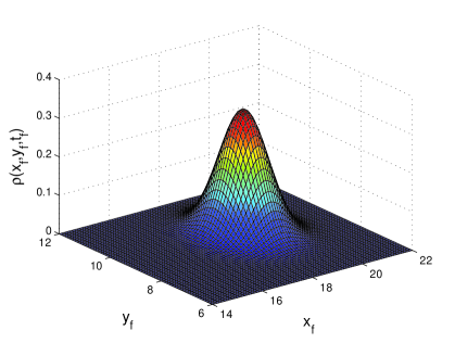
Figure 1: Plot of the joint distribution function $\rho(x_{f},y_{f},t_{f})$ for the parameter values $D=0.05,\ \beta=10,$ $\tau_{r}=10,\ k=0.2,$ and $v=2$ at final time $t_{f}=20$.

To obtain the joint probability distribution $\rho(x_{f},y_{f},t_{f})$, we integrate the above expression over the initial points, assuming that the system was initially in thermal equilibrium with the joint probability distribution
$\rho(x_{0},y_{0})=\frac{\beta k}{2\pi}\ \exp\left(-\frac{\beta k}{2}[x_{0}^{2}+y_{0}^{2}]\right)$. So,

$$\rho(x_{f},y_{f},t_{f}) = \int\textrm{d}x_{0}\int\textrm{d}y_{0}\rho(x_{0},y_{0})P(x_{f},y_{f},t_{f}\mid x_{0},y_{0})$$ (25)

$$= \left(\frac{\beta k}{2\pi}\right)\ \exp\Bigl{[}-\frac{\beta k\textrm{e}^{-2t_{f}/\tau_{r}}}{2b^{2}}$$

$$\times\left(v^{2}\tau_{r}^{2}+p\textrm{e}^{2t_{f}/\tau_{r}}+2\textrm{e}^{t_{f}/\tau_{r}}v\tau_{r}q\right)\Bigr{]},$$

where

$$p = v^{2}t_{f}^{2}b+2\tau_{r}vx_{f}-2\sigma^{2}\tau_{r}^{3}vx_{f}+(x_{f}^{2}+y_{f}^{2})(1+\sigma^{4}\tau_{r}^{4})$$ (26)

$$+\tau_{r}^{2}[v^{2}+4\sigma vy_{f}+2\sigma^{2}(x_{f}^{2}+y_{f}^{2})]-2t_{f}vx_{f}$$

$$-2t_{f}v^{2}\tau_{r}-2t_{f}v\tau_{r}\sigma[y_{f}+\sigma\tau_{r}(x_{f}+\sigma\tau_{r}y_{f})],$$

$$q = \cos(\sigma t_{f})[vt_{f}-x_{f}+\tau_{r}(-v+\sigma^{2}\tau_{r}x_{f}-2\sigma y_{f})]$$ (27)

$$+\sin(\sigma t_{f})[-y_{f}+\sigma\tau_{r}(-vt_{f}+2x_{f}+\sigma\tau_{r}y_{f})].$$

During simplifications, we have used the relation, $\beta Dk\tau_{r}=1$. For a particular set of parameter values, the joint probability density $\rho(x_{f},y_{f},t_{f})$ is plotted in Fig.(1).

The marginal probability is defined as the probability of finding the particle at a given $x_{f}$ or $y_{f}$ for arbitrary values of $y_{f}$ or $x_{f}$, respectively. After integrating $\rho(x_{f},y_{f},t_{f})$ with respect to the appropriate end point variable, the marginal probability distributions are found as

$$\rho(x_{f},t_{f}) = \int\textrm{d}y_{f}\ \rho(x_{f},y_{f},t_{f})$$ (28)

$$= \left(\frac{k\beta}{2\pi}\right)^{1/2}\exp\biggl{\{}-\frac{k\beta\ \textrm{e}^{-2t_{f}/\tau_{r}}}{2b^{4}}$$

$$\times\left(-v\ \textrm{e}^{t_{f}/\tau_{r}}[t_{f}b-\tau_{r}+\sigma^{2}\tau_{r}^{3}]+\textrm{e}^{t_{f}/\tau_{r}}x_{f}b^{2}+v\tau_{r}\left[(-1+\sigma^{2}\tau_{r}^{2})\cos(\sigma t_{f})+2\sigma\tau_{r}\sin(\sigma t_{f})\right]\right)^{2}\biggr{\}},$$

and

$$\rho(y_{f},t_{f}) = \int\textrm{d}x_{f}\ \rho(x_{f},y_{f},t_{f})$$ (29)

$$= \left(\frac{k\beta}{2\pi}\right)^{1/2}\exp\biggl{\{}-\frac{k\beta\ \textrm{e}^{-2t_{f}/\tau_{r}}}{2b^{4}}$$

$$\times\left(-v\sigma\tau_{r}\ \textrm{e}^{t_{f}/\tau_{r}}\left[t_{f}b-2\tau_{r}\right]+y_{f}\ \textrm{e}^{t_{f}/\tau_{r}}\ b^{2}+v\tau_{r}\left[-2\sigma\tau_{r}\cos(\sigma t_{f})+(-1+\sigma^{2}\tau_{r}^{2})\sin(\sigma t_{f})\right]\right)^{2}\biggr{\}}.$$

Eqs. (25), (28) and (29) are the main results of this section.

4 Generalized Onsager-Machlup Lagrangian and stochastic thermodynamic quantities

In this section, we establish an energy-balance relation and a second law type formulation valid for a single trajectory. We consider that, for every forward trajectory $[x(t),y(t)]$ specifying the system’s evolution over time interval $[-\tau,\tau]$, there exists a time-reversed trajectory $[x^{\dagger}(t),y^{\dagger}(t)]$ over the same interval. The probability measure of the forward path could be expressed in terms of the transition probability up to a normalization factor as,

$$P_{F}(x(\tau),y(\tau)\mid x(-\tau),y(-\tau))$$

$$\sim\exp\left(-\int_{-\tau}^{\tau}{\cal L}(x,y,\dot{x},\dot{y},t)\,\textrm{d}t\right),$$ (30)

with the generalized Onsager-Machlup Lagrangian ${\cal L}(x,y,\dot{x},\dot{y},t)$ as given in Eq.(10). Similarly, the transition probability corresponding to the time reversed trajectory is expressed as taniguchi ; cohen

$$P_{R}(x^{\dagger}(\tau),y^{\dagger}(\tau)\mid x^{\dagger}(-\tau),y^{\dagger}(-\tau))$$

$$\sim\exp\Biggl{(}-\int_{-\tau}^{\tau}{\cal L}^{\dagger}(x^{\dagger},y^{\dagger},\dot{x}^{\dagger},\dot{y}^{\dagger},t)\,\textrm{d}t\Biggr{)},$$ (31)

where ${\cal L}^{\dagger}$ is obtained from ${\cal L}$ under the time-reversal changes $v\rightarrow-v,\ x^{\dagger}(t)\rightarrow x(-t),\ \dot{x}^{\dagger}(t)\rightarrow-\dot{x}(-t),\ y^{\dagger}(t)\rightarrow y(-t)$ and $\dot{y}^{\dagger}(t)\rightarrow-\dot{y}(-t)$.

4.1 Entropy production in the medium

The ratio of the transition probability for the forward trajectory to that of the reversed trajectory is given by

$$\frac{P_{F}(x(\tau),y(\tau)\mid x(-\tau),y(-\tau))}{P_{R}(x^{\dagger}(\tau),y^{\dagger}(\tau)\mid x^{\dagger}(-\tau),y^{\dagger}(-\tau))}$$

$$=\exp\left[-\int_{-\tau}^{\tau}({\cal L}-{\cal L}^{\dagger})\,\textrm{d}t\right],$$ (32)

where

$${\cal L}-{\cal L}^{\dagger}=\beta\left[k\dot{x}(x-vt)+k\dot{y}y+n\dot{x}y-n\dot{y}x\right].$$ (33)

The entropy production in the medium $\Delta S_{m}$ satisfies the detailed fluctuation theorem park1

$$\Delta S_{m}=k_{B}\ \ln\left(\frac{P_{F}(x(\tau),y(\tau)\mid x(-\tau),y(-\tau))}{P_{R}(x^{\dagger}(\tau),y^{\dagger}(\tau)\mid x^{\dagger}(-\tau),y^{\dagger}(-\tau))}\right),$$ (34)

From relation (32) and (33), we have

$$\Delta S_{m}=\frac{1}{T}\Biggl{[}-\Delta U+\int_{-\tau}^{\tau}\frac{\partial U}{\partial t}\textrm{d}t+\int_{-\tau}^{\tau}(-n\dot{x}y+n\dot{y}x)\textrm{d}t\Biggr{]},$$ (35)

where $\Delta U=U(x(\tau),y(\tau))-U(x(-\tau),y(-\tau))$ is the change in the potential energy and the explicit form of the second term is

$$\int_{-\tau}^{\tau}\frac{\partial U}{\partial t}dt=-kv\int_{-\tau}^{\tau}(x-vt).$$ (36)

4.2 Work and dissipated heat

Since the heat transferred to the medium is ${\cal Q}=T\Delta S_{m}$, we use Eq. (35) to find

$${\cal Q}=\left[-\Delta U+\int_{-\tau}^{\tau}\frac{\partial U}{\partial t}\ \textrm{d}t\ +\int_{-\tau}^{\tau}(-n\dot{x}y+n\dot{y}x)\ \textrm{d}t\right]$$

$$=-\Delta U+{\cal W}_{\rm tr}+{\cal W}_{\rm m}.$$ (37)

In the last equality, the dissipated heat is expressed in terms of the change in the potential energy and the work that consists of two parts, namely, the thermodynamic work, ${\cal W}_{\rm tr}=\int_{-\tau}^{\tau}\frac{\partial U}{\partial t}\ \textrm{d}t$, which is the work done on the system by the harmonic trap sekimoto ; mazonka ; zon_cohen1 ; zon_cohen2 and the mechanical work, ${\cal W}_{\rm m}=\int_{-\tau}^{\tau}(-n\dot{x}y+n\dot{y}x)\ \textrm{d}t$. Similar partition of the total work into physically meaningful works can be found in recent literatures pjop ; ciliberto2 ; hanggi . For further discussions on various definitions of work and their behavior under gauge transformation, readers are referred to hanggi . Together with these definitions, Eq.(37) becomes the statement of the energy conservation principle valid on each trajectory seifert ; seifert1 ; sekimoto .

Next, to show the second law type formulation for the medium entropy production in the framework of the Onsager-Machlup theory taniguchi ; cohen , we split the Lagrangian ${\cal L}$ into time reversal symmetric, ${\cal L}^{\rm r}={\cal L}+{\cal L}^{\dagger}$, and anti-symmetric, ${\cal L}^{\rm ir}={\cal L}-{\cal L}^{\dagger}$, components and arrive at

$${\cal L}=\frac{1}{2}\left[{\cal L}^{\rm r}+{\cal L}^{\rm ir}\right]\ =\frac{1}{2}\left[{\cal L}^{\rm r}-\Delta\dot{S}_{m}/k_{B}\right].$$ (38)

Using Eqs. (32) and (34), ${\cal L}^{\rm ir}$ in the above equation has been replaced by the rate of entropy production $\Delta\dot{S}_{m}$. It is evident from Eq.(10) that the average path described by

$$\left\langle\dot{x}\right\rangle+(\left\langle x\right\rangle-vt)/\tau_{r}+\sigma\left\langle y\right\rangle=0,$$ (39)

$$\left\langle\dot{y}\right\rangle+\left\langle y\right\rangle/\tau_{r}-\sigma\left\langle x\right\rangle=0,$$ (40)

corresponds to the minimum value of the integral $\int_{0}^{t_{f}}{\cal L}(x,y,\dot{x},\dot{y},t)\,\textrm{d}t$. Substituting (39) and (40) into the relation

$${\cal L}^{\rm r}\left(\langle\dot{x}\rangle,\langle x\rangle,\langle\dot{y}\rangle,\langle y\rangle,t\right)=\Delta\dot{S}_{m}\left(\langle\dot{x}\rangle,\langle x\rangle,\langle\dot{y}\rangle,\langle y\rangle,t\right)/k_{B},$$ (41)

we find

$${\cal L}^{\rm r} = \frac{1}{4D}\left[\langle\dot{x}\rangle-(\langle x\rangle-vt)/\tau_{r}-\sigma\langle y\rangle\right]^{2}$$ (42)

$$+\frac{1}{4D}\left[-\langle\dot{y}\rangle+\langle y\rangle/\tau_{r}-\sigma\langle x\rangle\right]^{2}>0;$$

Eq. (42), ensuring $\Delta\dot{S}_{m}\left(\langle\cdots\rangle\right)>0$, shows the consistency with the second law of thermodynamics.

5 Distribution of the work performed by the moving trap

In this section, we derive the distribution of the work done by the harmonic trap on the Brownian particle. The work done or the energy put into the system by the trapping potential over time $[0:t_{f}]$ is

$${\cal W}_{\rm tr}[x(t)]=-kv\int_{0}^{t_{f}}(x-vt)\,{\rm d}t.$$ (43)

In order to obtain the distribution of this work, we need to perform functional averages of this quantity over all possible paths $\left[x(t),y(t);0\leq t\leq t_{f}\right]$ as well as integrals over the initial and final points farago ; taniguchi ; cohen of the path. The probability measure of such a path is given by,

$${\cal P}\left[x(t),y(t);0\leq t\leq t_{f}\right]\sim\exp\left(-\int_{0}^{t_{f}}{\cal L}(x,y,\dot{x},\dot{y},t)\,\textrm{d}t\right).$$ (44)

So, the probability distribution of the work performed by the trap, henceforth denoted as $W_{\rm tr}$, is

$$P(W_{\rm tr})=\left\langle\delta\left(W_{\rm tr}-\left\{-kv\int_{0}^{t_{f}}(x-vt)\,{\rm d}t\right\}\right)\right\rangle$$

$$=\int\textrm{d}x_{0}\int\textrm{d}y_{0}\ \rho(x_{0},y_{0})\int\textrm{d}x_{f}\int\textrm{d}y_{f}$$

$$\times\int{\cal D}[x(t)]\int{\cal D}[y(t)]\ {\cal P}\left[x(t),y(t)\right]$$

$$\times\delta\left(W_{\rm tr}-\left\{-kv\int_{0}^{t_{f}}(x-vt)\,{\rm d}t\right\}\right)$$

$$=\frac{\beta}{2\pi}\int_{-\infty}^{\infty}\textrm{d}\lambda\,\textrm{e}^{\textrm{i}\lambda\beta W_{\rm tr}}\ P(\textrm{i}\lambda W_{\rm tr});$$ (45)

where

$$P(\textrm{i}\lambda W_{\rm tr})=\int\textrm{d}x_{0}\int\textrm{d}y_{0}\ \rho(x_{0},y_{0})\int\textrm{d}x_{f}\int\textrm{d}y_{f}$$

$$\times\int{\cal D}[x(t)]\int{\cal D}[y(t)]\ \exp\left(-\int_{0}^{t_{f}}{\cal L}_{M}(x,y,\dot{x},\dot{y},\lambda)\,\textrm{d}t\right),$$ (46)

with

$${\cal L}_{M}(x,y,\dot{x},\dot{y},\lambda)=\frac{1}{4D}\Bigl{\{}\left[\dot{x}+(x-vt)/\tau_{r}+\sigma y\right]^{2}$$

$$+\left[\dot{y}+y/\tau_{r}-\sigma x\right]^{2}-4\textrm{i}\lambda v(x-vt)/\tau_{r}\Bigr{\}}.$$ (47)

In order to derive the distribution function at a finite time, we consider the system to have evolved from the initial equilibrium distribution, $\rho(x_{0},y_{0})=\frac{\beta k}{2\pi}\ \exp\left(-\frac{\beta k}{2}[x_{0}^{2}+y_{0}^{2}]\right)$.

To evaluate the functional integrals in (46), we follow the variational approach discussed earlier in section 3. We seek the most probable trajectory $(\tilde{x}(t)$, $\tilde{y}(t))$ which corresponds to the largest contribution to the path integral. The extremization condition, $\delta\int_{0}^{t_{f}}{\cal L}_{M}\,\textrm{d}t=0$, leads to two Euler-Lagrange equations

$$\ddot{\tilde{x}}+2\sigma\dot{\tilde{y}}-(\sigma^{2}+1/\tau_{r}^{2})\tilde{x}-v(1-2\textrm{i}\lambda)/\tau_{r}+vt/\tau_{r}^{2}=0,$$ (48)

$$\ddot{\tilde{y}}-(\sigma^{2}+1/\tau_{r}^{2})\tilde{y}-2\sigma\dot{\tilde{x}}+v\sigma t/\tau_{r}=0,$$ (49)

which are supplemented with the boundary conditions, $\tilde{x}(t=0)=x_{0},\ \tilde{x}(t=t_{f})=x_{f},\ \tilde{y}(t=0)=y_{0}$ and $\tilde{y}(t=t_{f})=y_{f}$. After some simplifications, the two Euler-Lagrange equations can be expressed in terms of higher derivatives of a single variable only. These are

$$\ddddot{\tilde{y}}+2\left(\sigma^{2}-1/\tau_{r}^{2}\right)\ddot{\tilde{y}}+\left(\sigma^{2}+1/\tau_{r}^{2}\right)^{2}\tilde{y}$$

$$-\left(\sigma^{2}+1/\tau_{r}^{2}\right)v\sigma t/\tau_{r}+2\sigma v/\tau_{r}^{2}=0\ ,$$ (50)

$$\left(\sigma^{2}+1/\tau_{r}^{2}\right)\tilde{x}= \frac{1}{2\sigma}\left[\dddot{\tilde{y}}-(\sigma^{2}+1/\tau_{r}^{2})\dot{\tilde{y}}+v\sigma/\tau_{r}\right]$$

$$+2\sigma\dot{\tilde{y}}-v\bar{\lambda}/\tau_{r}+vt/\tau_{r}^{2}\ ,$$ (51)

where, $\bar{\lambda}=1-2\textrm{i}\lambda$. The optimal solutions are

$$\tilde{x}(t)= v\left[bt-\bar{\lambda}\tau_{r}-(\bar{\lambda}-2)\sigma^{2}\tau_{r}^{3}\right]/b^{2}$$

$$+\cosh(t/\tau_{r})\left[c_{2}\cos(\sigma t)-c_{1}\sin(\sigma t)\right]$$

$$+\sinh(t/\tau_{r})\left[c_{4}\cos(\sigma t)-c_{3}\sin(\sigma t)\right],$$ (52)

$$\tilde{y}(t)= \sigma\tau_{r}v[bt-2\tau_{r}]/b^{2}+\cosh(t/\tau_{r})[c_{1}\cos(\sigma t)+c_{2}\sin(\sigma t)]$$

$$+\sinh(t/\tau_{r})[c_{3}\cos(\sigma t)+c_{4}\sin(\sigma t)].$$ (53)

The explicit dependence of the constants $c_{1},\ c_{2},\ c_{3}$ and $c_{4}$ on the boundary conditions and other parameters of the problem is shown in appendix B. Incorporating the quadratic term arising from the fluctuations around the most probable path, we write Eq.(46) as,

$$P(\textrm{i}\lambda W_{\rm tr}) =\phi(t_{f})\int\textrm{d}x_{0}\int\textrm{d}y_{0}\ \rho(x_{0},y_{0})\int\textrm{d}x_{f}$$

$$\times\int\textrm{d}y_{f}\ \exp\left(-\int_{0}^{t_{f}}{\cal L}_{M}(\tilde{x},\tilde{y},\dot{\tilde{x}},\dot{\tilde{y}},\lambda)\,\textrm{d}t\right).$$ (54)

Substituting the solutions (52) and (53) into (54) and subsequently performing first the integral over time and then over final and initial positions (some of the intermediate calculations are shown in appendix B), we have

$$P(\textrm{i}\lambda W_{\rm tr})=\exp\left[-\left(W_{0}\lambda^{2}+\textrm{i}\bar{W}\lambda\right)\right],$$ (55)

where

$$W_{0} = \frac{v^{2}\textrm{e}^{-t_{f}/\tau_{r}}}{Db^{2}}\Bigl{\{}\textrm{e}^{t_{f}/\tau_{r}}\left[bt_{f}-\tau_{r}+\sigma^{2}\tau_{r}^{3}\right]$$ (56)

$$+\cos(\sigma t_{f})\left[\tau_{r}-\sigma^{2}\tau_{r}^{3}\right]-2\sigma\tau_{r}^{2}\sin(\sigma t_{f})\Bigr{\}};$$

$$\bar{W} = \frac{v^{2}\textrm{e}^{-t_{f}/\tau_{r}}}{2Db^{3}}\Bigl{\{}\textrm{e}^{t_{f}/\tau_{r}}\bigl{[}-2\tau_{r}+6\sigma^{2}\tau_{r}^{3}+\sigma^{2}b^{2}t_{f}^{2}\tau_{r}$$ (57)

$$+2t_{f}(1-\sigma^{4}\tau_{r}^{4})\bigr{]}+\cos(\sigma t_{f})\left[2\tau_{r}-6\sigma^{2}\tau_{r}^{3}\right]$$

$$+2\sigma\tau_{r}^{2}\sin(\sigma t_{f})\left[\sigma^{2}\tau_{r}^{2}-3\right]\Bigr{\}}.$$

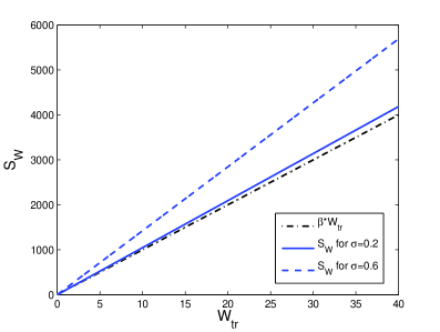
Figure 2: Plot of the symmetry function with $W_{\rm tr}$ for the parameter values $D=0.01,\ \beta=100,$ $\tau_{r}=0.5,\ k=2,$ and $v=2$, at the final time $t_{f}=6$. The dashed-dot line corresponds to the situation where the symmetry function follows the fluctuation theorem. The deviation from the fluctuation relation increases for larger values of $\sigma$.

Substituting (55) into Eq.(45) and doing the final Gaussian integral over $\lambda$, we find the final form of the work distribution as

$$P(W_{\rm tr})=\left(\frac{\beta^{2}}{4\pi W_{0}}\right)^{1/2}\ \exp\left[-\frac{(\beta W_{\rm tr}-\bar{W})^{2}}{4W_{0}}\right].$$ (58)

The known result of the work distribution function for a uniformly dragged colloidal particle mazonka ; zon_cohen1 ; zon_cohen2 ; seifert3 ; imparato3 can be retrieved by substituting $\sigma=0$ in our general result. The work distribution function, in this case, obeys the fluctuation theorem. The symmetry function defined as $S_{W}=\ln\left[\frac{P(W_{\rm tr})}{P(-W_{\rm tr})}\right]$, therefore, has a value $S_{W}=\beta W_{\rm tr}$. In the presence of the non conserving force ($\sigma\neq 0$), the symmetry function is

$$S_{W}=\beta W_{\rm tr}\bar{W}/W_{0}.$$ (59)

Clearly it does not satisfy the conventional fluctuation theorem since to hold this relation, it is required that $S_{W}=\beta W_{\rm tr}$. The present work distribution function satisfies the fluctuation theorem if $W_{0}=\bar{W}$. Given the following expressions for $W_{0}$ and $\bar{W}$

$$W_{0}\approx\frac{v^{2}}{Db^{2}}\left[bt_{f}-\tau_{r}+\sigma^{2}\tau_{r}^{3}\right],$$ (60)

$$\bar{W}\approx\frac{v^{2}}{2Db^{3}}\left[-2\tau_{r}+6\sigma^{2}\tau_{r}^{3}+\sigma^{2}b^{2}t_{f}^{2}\tau_{r}+2t_{f}(1-\sigma^{4}\tau_{r}^{4})\right],$$ (61)

in the steady state limit $t_{f}/\tau_{r}>>1$, such a condition is satisfied if

$$\sigma^{2}\tau_{r}\left[6\tau_{r}^{2}-2\sigma^{2}\tau_{r}^{4}+t_{f}^{2}b^{2}-4t_{f}\tau_{r}b\right]=0.$$ (62)

$\sigma=0$ trivially satisfies this equation. The other nonzero values of $\sigma$ for which Eq. (62) is satisfied are

$$\sigma_{1}=\frac{1}{t_{f}\tau_{r}}\left[2t_{f}\tau_{r}-t_{f}^{2}+\tau_{r}^{2}-\tau_{r}^{2}\sqrt{(-4(\frac{t_{f}}{\tau_{r}})^{2}+4\frac{t_{f}}{\tau_{r}}+1})\right]^{\frac{1}{2}}$$

$$=-\sigma_{2};$$ (63)

$$\sigma_{3}=\frac{1}{t_{f}\tau_{r}}\left[2t_{f}\tau_{r}-t_{f}^{2}+\tau_{r}^{2}+\tau_{r}^{2}\sqrt{(-4(\frac{t_{f}}{\tau_{r}})^{2}+4\frac{t_{f}}{\tau_{r}}+1})\right]^{\frac{1}{2}}$$

$$=-\sigma_{4}.$$ (64)

In the steady state limit ($t_{f}/\tau_{r}>>1$), these roots become complex and hence not physically acceptable. To see the deviation from the fluctuation theorem, we have plotted the symmetry function as a function of $W_{\rm tr}$ for different values of $\sigma$ (see figure (2)). The deviation becomes more prominent as one increases the value of $\sigma$.

6 Summary and perspectives

In this article, we have studied the two dimensional motion of a Brownian particle subject to a time dependent harmonic force and a nonconservative rotational torque. Starting with the overdamped Langevin equations, we have obtained a path integral description for the transition probability of the Brownian particle. The transition probability gives the probability of finding the Brownian particle at a final position at time $t_{f}$ given that it was at a specific position at an earlier time $t_{0}$. Using a variational method, we evaluate the path integral to obtain the explicit form of the transition probability. This, upon integration over the initial position coordinates gives the joint probability distribution.

In order to obtain the definitions of the work, the dissipated heat and the entropy production of the medium, we consider the forward and time-reversed trajectories of the particle. Here, the time reversed trajectory is characterized by the reversal of the velocity variables and the flipping of the end points with the same underlying dynamics. After identifying the medium entropy production and the dissipated heat, we obtain the energy conservation relation and, subsequently, define the two works; one done by the moving trap and the other by the nonconservative force. Further, we show that the average path corresponding to the minimum of the generalized Lagrangian leads to the positive entropy production rate.

The expression of the thermodynamic work further allows us to derive its distribution function using a similar path integral approach adopted for the transition probability. We expressed the distribution function in a functional integral form which was approximated by the maximum contribution coming from the optimal path and the fluctuations upto second order about the optimal path. The distribution is Gaussian in nature. The explicit form of the distribution correctly produces the known result of the work distribution for a dragged Brownian particle in the absence of any other force ($\sigma=0$). However, in the presence of the nonconservative force, its mean and variance have a non-trivial oscillatory dependence with $\sigma$ as the angular frequency. As a consequence, the work distribution fails to satisfy the conventional work fluctuation relation.

In this context, we discuss another version of the model where the thermodynamic work naturally appears as a ratio of the forward and reverse process and satisfies fluctuation relation. Here, the nonconservative force is applied at the position of the minimum of the moving harmonic trap. In the reference frame of the trap, the particle moving under the potential $\phi(X,y)=k(X^{2}+y^{2})/2$, satisfies the overdamped Langevin equations given by,

$$\dot{X}=-X/\tau_{r}-v-\sigma y+\xi_{x}/\alpha,$$ (65)

$$\dot{y}=-y/\tau_{r}+\sigma X+\xi_{y}/\alpha,$$ (66)

with, $X=x-vt$.

To obtain the thermodynamic work and its fluctuation relation, we consider the time reversed process with the reversal of sign in appropriate terms of the above equations vladimir . The corresponding Lagrangian, denoted by $L^{R}$, has the form

$$L^{R}=\frac{1}{4D}\left[(-\dot{X}+X/\tau_{r}-v-\sigma y)^{2}+(-\dot{y}+y/\tau_{r}+\sigma X)^{2}\right].$$ (67)

It is straightforward to obtain the ratio of the forward and reverse transition probabilities as

$$\frac{P_{F}}{P_{R}}=\exp\left[\beta\left(-\Delta\phi-kv\int X\,\textrm{d}t\right)\right].$$ (68)

The first term in the argument of the exponential stands for the change in the potential energy and the second term can be recognized as the thermal work done jarzynskirel . If we consider the initial distribution to be a canonical one, i.e. $\rho_{0}\propto e^{-\beta\phi(X_{0},y_{0})}$, then the ratio of forward and reverse probability densities yields the fluctuation relation for the work ${\cal W}_{\rm tr}=\int-kvX\,\textrm{d}t$,

$$\frac{{\cal P}_{F}}{{\cal P}_{R}}=\exp\left(\beta{\cal W_{\rm tr}}\right),$$ (69)

where the probability measure of the path starting at a given initial point is obtained from the transition probability as ${\cal P}_{F,R}=\rho_{0}\ P_{F,R}$. In this context, it will be of interest to verify whether the distribution of this work satisfies various aspects of fluctuation relations and will be discussed elsewhere.

Finally, the model studied in this paper and its extension seem to be promising for further investigations and the results obtained would also be amenable to experimental verifications.

Appendix A Path integral solution of the Fokker-Planck equation

The joint probability density function $\rho(x,y,t+\varepsilon)$ at time $t+\varepsilon$ is related to the transition probability
$P(x,y,t+\varepsilon\mid x^{\prime},y^{\prime},t)$ as

$$\rho(x,y,t+\varepsilon)=\int P(x,y,t+\varepsilon\mid x^{\prime},y^{\prime},t)\ \rho(x^{\prime},y^{\prime},t)\,\textrm{d}x^{\prime}\,\textrm{d}y^{\prime}.$$ (70)

For infinitesimal time difference $\varepsilon$, the transition probability can be expressed as,

$$P(x,y,t+\varepsilon\mid x^{\prime},y^{\prime},t)\approx\left[1+\hat{L}_{\rm FP}\cdot\varepsilon+{\it O}(\varepsilon^{2})\right]\delta(x-x^{\prime})\ \delta(y-y^{\prime}).$$ (71)

Using the Fourier representation of the $\delta$ function and substituting $\hat{L}_{\rm FP}$ from Eq.(6), we have,

$$P(x,y,t+\varepsilon\mid x^{\prime},y^{\prime},t)=\frac{1}{(2\pi)^{2}}\int_{-\infty}^{\infty}\textrm{d}q_{1}\int_{-\infty}^{\infty}\textrm{d}q_{2}\biggl{\{}1+\varepsilon((x^{\prime}-vt)/\tau_{r}+\sigma y^{\prime})\frac{\partial}{\partial x}+\varepsilon D\frac{\partial^{2}}{\partial x^{2}}$$

$$-\varepsilon(-y^{\prime}/\tau_{r}+\sigma x^{\prime})\frac{\partial}{\partial y}+\varepsilon D\frac{\partial^{2}}{\partial y^{2}}\biggr{\}}\ \exp\left[\textrm{i}\left(q_{1}(x-x^{\prime})+q_{2}(y-y^{\prime})\right)\right]$$

$$=\frac{1}{4\pi D\varepsilon}\ \exp\Biggl{\{}-\frac{1}{4D}\left(\left[\frac{(x-x^{\prime})}{\varepsilon}+(x^{\prime}-vt)/\tau_{r}+\sigma y^{\prime}\right]^{2}\varepsilon+\left[\frac{(y-y^{\prime})}{\varepsilon}+y^{\prime}/\tau_{r}-\sigma x^{\prime}\right]^{2}\varepsilon\right)\Biggr{\}}.$$ (72)

In order to obtain the transition probability for a finite time difference $(t_{f}-t_{0})$, we divide the time difference into $N$ small segments of duration $\varepsilon=(t_{f}-t_{0})/N$ . Then, in the limit $N\rightarrow\infty$ and $\varepsilon\rightarrow 0$, the repetitive application of the Chapman-Kolmogorov equation risken yields,

$$P(x_{f},y_{f},t_{f}\mid x_{0},y_{0},t_{0}) = \int\prod_{i=1}^{N}\frac{\textrm{d}x_{i}}{(4\pi D\varepsilon)^{1/2}}\int\prod_{i=1}^{N}\frac{\textrm{d}y_{i}}{(4\pi D\varepsilon)^{1/2}}$$

$$\times\exp\biggl{\{}-\sum_{i=1}^{N}\frac{1}{4D}\left(\left[(x_{i}-x_{i-1})/\varepsilon+(x_{i}-vt_{i})/\tau_{r}+\sigma y_{i}\right]^{2}+\left[(y_{i}-y_{i-1})/\varepsilon+y_{i}/\tau_{r}-\sigma x_{i}\right]^{2}\right)\,\varepsilon\biggr{\}}$$

$$= \int{\cal D}[x(t)]\int{\cal D}[y(t)]\,\exp\biggl{\{}-\int_{t_{0}}^{t_{f}}\frac{1}{4D}\left(\left[\dot{x}+(x-vt)/\tau_{r}+\sigma y\right]^{2}+\left[\dot{y}+y/\tau_{r}-\sigma x\right]^{2}\right)\,\textrm{d}t\biggr{\}}.$$

Appendix B Some intermediate calculations of section 5

After substituting the optimal solutions (52) and (53) into Eq.(47), the expression of the modified Lagrangian reads

$${\cal L}_{M}(\tilde{x},\tilde{y},\dot{\tilde{x}},\dot{\tilde{y}},\lambda) = \frac{1}{4D\tau_{r}^{2}b^{2}}\bigl{\{}(-1+\bar{\lambda})v\tau_{r}-\textrm{e}^{t/\tau_{r}}b\left[(c_{2}+c_{4})\cos(\sigma t)-(c_{1}+c_{3})\sin(\sigma t)\right]\bigr{\}}^{2}$$ (74)

$$+ \frac{1}{4D\tau_{r}^{2}b^{2}}\bigl{\{}(-1+\bar{\lambda})\sigma\tau_{r}^{2}v+\textrm{e}^{t/\tau_{r}}b\left[(c_{1}+c_{3})\cos(\sigma t)+(c_{2}+c_{4})\sin(\sigma t)\right]\bigr{\}}^{2}$$

$$+ \frac{(\bar{\lambda}-1)v}{2D\tau_{r}}\biggl{\{}-\tau_{r}v[\bar{\lambda}b+\sigma^{2}t\tau_{r}b-2\sigma^{2}\tau_{r}^{2}]/b^{2}+\cosh(t/\tau_{r})[c_{2}\cos(\sigma t)-c_{1}\sin(\sigma t)]$$

$$+\sinh(t/\tau_{r})[c_{4}\cos(\sigma t)-c_{3}\sin(\sigma t)]\biggr{\}}.$$

where, $c_{1},\ c_{2},\ c_{3}$ and $c_{4}$ have the form

$$c_{1}=y_{0}+2\sigma\tau_{r}^{2}v/b^{2},$$ (75)

$$c_{2}=x_{0}+v\tau_{r}(\bar{\lambda}b-2\sigma^{2}\tau_{r}^{2})/b^{2},$$ (76)

$$c_{3}=\frac{1}{b^{2}}\biggl{\{}-\coth(t_{f}/\tau_{r})[y_{0}b^{2}+2\sigma\tau_{r}^{2}v]+{\rm csch}(t_{f}/\tau_{r})\bigl{[}-\sigma\tau_{r}v(t_{f}b-2\tau_{r})\cos(\sigma t_{f})+y_{f}b^{2}\cos(\sigma t_{f})$$

$$+v\sin(\sigma t_{f})(t_{f}b-\bar{\lambda}\tau_{r}b+2\sigma^{2}\tau_{r}^{3})-x_{f}b^{2}\sin(\sigma t_{f})\bigr{]}\biggr{\}},$$ (77)

$$c_{4}=\frac{1}{b^{2}}\biggl{\{}-\coth(t_{f}/\tau_{r})[v\tau_{r}(\bar{\lambda}b-2\sigma^{2}\tau_{r}^{2})+x_{0}b^{2}]+{\rm csch}(t_{f}/\tau_{r})\bigl{[}v\tau_{r}(\bar{\lambda}b-2\sigma^{2}\tau_{r}^{2})\cos(\sigma t_{f})+(x_{f}b^{2}-vt_{f}b)\cos(\sigma t_{f})$$

$$+y_{f}b^{2}\sin(\sigma t_{f})-\sigma\tau_{r}v(t_{f}b-2\tau_{r})\sin(\sigma t_{f})\bigr{]}\biggl{\}}.$$ (78)

We use the above expressions in Eq.(54) to evaluate various integrations. After performing the time integration and integrations over the final positions, we have

$$P(\textrm{i}\lambda W_{\rm tr}) = \int\textrm{d}x_{0}\int\textrm{d}y_{0}\ \rho(x_{0},y_{0})\ \exp\bigl{\{}-v\textrm{e}^{-t_{f}/\tau_{r}}(1-\bar{\lambda})[h_{1}x_{0}+h_{2}y_{0}+h_{3}]/(4Db^{3})\bigr{\}}$$ (79)

$$= \frac{\beta k}{2\pi}\exp\left(-v\textrm{e}^{-t_{f}/\tau_{r}}(1-\bar{\lambda})h_{3}/(4Db^{3})\right)\int\textrm{d}x_{0}\exp\biggl{\{}-\left[\beta kx_{0}^{2}/2+v\textrm{e}^{-t_{f}/\tau_{r}}(1-\bar{\lambda})h_{1}x_{0}/(4Db^{3})\right]\biggr{\}}$$

$$\times\int\textrm{d}y_{0}\exp\biggl{\{}-\left[\beta ky_{0}^{2}/2+v\textrm{e}^{-t_{f}/\tau_{r}}(1-\bar{\lambda})h_{2}y_{0}/(4Db^{3})\right]\biggr{\}},$$

where $h_{1},\ h_{2}$ and $h_{3}$ are

$$h_{1}=-2b^{2}\left[\cosh(t_{f}/\tau_{r})-\cos(\sigma t_{f})+\sigma\tau_{r}\sin(\sigma t_{f})+\sinh(t_{f}/\tau_{r})\right],$$ (80)

$$h_{2}=-2b^{2}\left[\sigma\tau_{r}\cos(\sigma t_{f})-\sigma\tau_{r}\textrm{e}^{t_{f}/\tau_{r}}+\sin(\sigma t_{f})\right],\ {\rm and}$$ (81)

$$h_{3}=2\tau_{r}v\cos(\sigma t_{f})[\bar{\lambda}b-4\sigma^{2}\tau_{r}^{2}]+v\cosh(t_{f}/\tau_{r})\left[8\sigma^{2}\tau_{r}^{3}-2\bar{\lambda}\tau_{r}b+\sigma^{2}t_{f}^{2}\tau_{r}b^{2}+bt_{f}(1+b\bar{\lambda}-3\sigma^{2}\tau_{r}^{2})\right]$$

$$-2\sigma\tau_{r}^{2}v\sin(\sigma t_{f})[2+b\bar{\lambda}-2\sigma^{2}\tau_{r}^{2}]+v\sinh(t_{f}/\tau_{r})\bigl{[}6\sigma^{2}\tau_{r}^{3}-(1+\bar{\lambda})\tau_{r}+(\bar{\lambda}-1)\sigma^{4}\tau_{r}^{5}$$

$$+\sigma^{2}t_{f}^{2}\tau_{r}b^{2}+t_{f}b(1+\bar{\lambda}b-3\sigma^{2}\tau_{r}^{2})\bigr{]}.$$ (82)

After doing the Gaussian integrals in Eq.(79) and using the relation $1/(D^{2}\beta k)=\tau_{r}/D$, we arrive at Eq.(55) in the main text.

References

- (1) R. Kubo, Rep. Prog. Phys. 29, 255 (1966)
- (2) R. Kubo, M. Toda, N. Hashitsume, Statistical Physics II : Nonequilibrium Statistical Mechanics, 2nd edn. (Springer, Berlin, 1998)
- (3) D. J. Evans, E. G. D. Cohen, G. P. Morriss, Phys. Rev. Lett. 71, 2401 (1993)
- (4) D. J. Evans, D. J. Searles, Phys. Rev. E 50, 1645 (1994)
- (5) G. Gallavotti, E. G. D. Cohen, Phys. Rev. Lett. 74, 2694 (1995)
- (6) J. Kurchan, J. Phys. A 31, 3719 (1998)
- (7) B. Derrida, J. Stat. Mech., P07023 (2007)
- (8) C. Jarzynski, Phys. Rev. Lett. 78, 2690 (1997); Phys. Rev. E 56,5018 (1997)
- (9) G. E. Crooks, Phys. Rev. E 60, 2721 (1999); Phys. Rev. E 61, 2361 (2000)
- (10) J. L. Lebowitz, H. Spohn, J. Stat. Phys. 95, 333 (1999)
- (11) R. J. Harris, G. M. Schütz, J. Stat. Mech. P07020 (2007)
- (12) U. Seifert, Phys. Rev. Lett. 95, 040602 (2005)
- (13) U. Seifert, Eur. Phys. J. B 64, 423 (2008)
- (14) U. Seifert, Rep. Prog. Phys. 75, 126001 (2012)
- (15) M. Esposito, C. Van den Broeck, Phys. Rev. Lett. 104, 090601 (2010)
- (16) Nonequilibrium Statistical Physics of Small Systems: Fluctuation Relations and Beyond, edited by R. Klages, W. Just, C. Jarzynski (Wiley-VCH, Weinheim, 2013)
- (17) R. van Zon, E. G. D. Cohen, Phys. Rev. Lett. 91, 110601 (2003)
- (18) R. van Zon, E. G. D. Cohen, Phys. Rev. E 67, 046102 (2003)
- (19) R. van Zon, E. G. D. Cohen, Phys. Rev. E 69, 056121 (2004)
- (20) F. Ritort, C. Bustamante, I. Tinoco, Jr., Proc. Natl Acad. Sci. USA 99, 13544 (2002)
- (21) O. Mazonka, C. Jarzynski, arXiv:cond-mat/9912121v1 (1999)
- (22) T. Speck, U. Seifert, Eur. Phys. J. B 43, 521 (2005)
- (23) A. Imparato, L. Peliti, G. Pesce, G. Rusciano, A. Sasso, Phys. Rev. E 76, 050101(R) (2007)
- (24) J. Farago, J. Stat. Phys. 107, 781 (2002)
- (25) A. Imparato, L. Peliti, Europhys. Lett. 70, 740 (2005)
- (26) S. Sabhapandit, Europhys. Lett. 96, 20005 (2011)
- (27) S. Sabhapandit, Phys. Rev. E 85, 021108 (2012)
- (28) C. Kwon, J. D. Noh, H. Park, Phys. Rev. E 83, 061145 (2011)
- (29) J. D. Noh, C. Kwon, H. Park, Phys. Rev. Lett. 111, 130601 (2013)
- (30) L. Onsager, S. Machlup, Phys. Rev. 91, 1505 (1953)
- (31) S. Machlup, L. Onsager, Phys. Rev. 91, 1512 (1953)
- (32) L. Bertini, A. De Sole, D. Gabrielli, G. Jona-Lasinio, C. Landim, Phys. Rev. Lett. 87, 040601 (2001)
- (33) L. Bertini, A. De Sole, D. Gabrielli, G. Jona-Lasinio, C. Landim, J. Stat. Phys. 107, 635 (2002)
- (34) L. Bertini, A. De Sole, D. Gabrielli, G. Jona-Lasinio, C. Landim, J. Stat. Phys. 123, 237 (2006)
- (35) A. Imparato, L. Peliti, Phys. Rev. E 74, 026106 (2006)
- (36) T. Taniguchi, E. G. D. Cohen, J. Stat. Phys. 126, 1 (2007); J. Stat. Phys. 130, 1 (2008); J. Stat. Phys. 130, 633 (2008)
- (37) E. G. D. Cohen, J. Stat. Mech., P07014 (2008)
- (38) C. Maes, K. Netočný, B. Wynants, J. Phys. A: Math. Theor. 42, 365002 (2009)
- (39) B. Saha, S. Mukherji, J. Stat. Mech., P08014 (2014)
- (40) A. Engel, Phys. Rev. E 80, 021120 (2009); D. Nickelsen, A. Engel, Eur. Phys. J. B 82, 207 (2011)
- (41) V. Y. Chernyak, M. Chertkov, C. Jarzynski, J. Stat. Mech., P08001 (2006)
- (42) S. Ciliberto, S. Joubaud, A. Petrosyan, J. Stat. Mech., P12003 (2010)
- (43) S. Joubaud, N. B. Garnier, S. Ciliberto, J. Stat. Mech., P09018 (2007)
- (44) H. Risken, The Fokker-Planck Equation : Methods of Solution and Applications (Springer-Verlag, Berlin, 1989)
- (45) F. W. Wiegel, Introduction to Path Integral Methods in Physics and Polymer Science (World Scientific, Singapore, 1986)
- (46) K. Sekimoto, Prog. Theor. Phys. Supp. 130, 17 (1998)
- (47) P. Jop, A. Petrosyan, S. Ciliberto, Europhys. Lett. 81, 50005 (2008)
- (48) M. Campisi, P. Hänggi, and P. Talkner, Rev. Mod. Phys. 83, 771 (2011)