Clustering of exceptional points and dynamical phase transitions

Abstract

The eigenvalues of a non-Hermitian Hamilton operator are complex and provide not only the energies but also the lifetimes of the states of the system. They show a non-analytical behavior at singular (exceptional) points (EPs). The eigenfunctions are biorthogonal, in contrast to the orthogonal eigenfunctions of a Hermitian operator. A quantitative measure for the ratio between biorthogonality and orthogonality is the phase rigidity of the wavefunctions. At and near an EP, the phase rigidity takes its minimum value. The lifetimes of two nearby eigenstates of a quantum system bifurcate under the influence of an EP. When the parameters are tuned to the point of maximum width bifurcation, the phase rigidity suddenly increases up to its maximum value. This means that the eigenfunctions become almost orthogonal at this point. This unexpected result is very robust as shown by numerical results for different classes of systems. Physically, it causes an irreversible stabilization of the system by creating local structures that can be described well by a Hermitian Hamilton operator. Interesting non-trivial features of open quantum systems appear in the parameter range in which a clustering of EPs causes a dynamical phase transition.

I Introduction

In its simplest form, the wavefunction of a quantum many-particle fermionic system can be written as a Slater determinant that satisfies the anti-symmetry requirements and consequently the Pauli principle. However, some corrections in the wavefunctions are usually necessary which are caused by their possible mixing. In nuclei, for example, corrections arise from the residual interaction between the particles of the system, with the consequence that the wavefunctions of all the states are strongly mixed. Another source is the interaction between system and environment into which the system is embedded. In this case, the states of the system interact via the common environment due to which their wavefunctions may be modified.

The natural environment of a localized quantum mechanical system is the extended continuum of scattering wavefunctions in which the system is embedded. This environment can be changed by means of external forces, however it can never be deleted. It causes some communication between distant levels, for details see the recent review ropp in which theoretical results are confronted with experimental results. The theoretical results are obtained by using a non-Hermitian Hamilton operator ${\cal H}$ for the description of the system, which contains explicitly the interaction between system and environment top . The eigenvalues and eigenfunctions of ${\cal H}$ differ essentially from those of a Hermitian Hamilton operator : the eigenfunctions are biorthogonal and the eigenvalues may show, as function of a certain parameter, deviations from Fermi’s golden rule. The differences between the eigenvalues and eigenfunctions of ${\cal H}$ and those of a Hermitian operator $H$ appear, above all, at and near to singular points at which two eigenvalues of ${\cal H}$ coalesce and the corresponding eigenfunctions differ from one another only by a phase. These singular points do not have any equivalent in the mathematics based on Hermitian Hamiltonians since the different eigenfunctions of $H$ are orthogonal (in contrast to those of ${\cal H}$, which are biorthogonal). These singular points are called usually exceptional points (EPs), according to kato .

The role of EPs in physical systems is considered in many papers during last years, e.g. mondragon ; pastawski ; mois2 ; atabek ; jolicard , see also the review top and the book moiseyev . In the present paper, we are interested in the relation of these singular points to phase transitions occurring in open quantum systems. Such a relation is first discussed theoretically some years ago in jumuro and hemuro , however without rigorous consideration of the biorthogonality of the eigenfunctions of ${\cal H}$. The same holds true for the papers pastawski on the dynamical phase transition observed experimentally and theoretically in the spin swapping operation in atomic systems. Only recently, the mixing of the wavefunctions at an EP and its relation to a dynamical phase transition is studied for an open quantum system with more than two states nearby2 . The states at both sides of the phase transition are not analytically related to one another, meaning that this characteristic feature of any phase transition is fulfilled. The theoretical results are compared to experimental results in the recent review ropp .

In contrast to these differences between Hermitian and non-Hermitian quantum physics at and near to an EP, the Hamilton operator of the Schrödinger equation of an open quantum system is almost Hermitian, to a good approximation, far from an EP. Here the eigenfunctions of the non-Hermitian Hamilton operator are almost orthogonal nearby1 ; and the system can be described quite well by a standard Hermitian Hamilton operator. We underline however that the Hamiltonian remains definitely non-Hermitian since the non-Hermiticity arises solely from the fact that the function space of the localized part of the system is a subsystem of the total function space : the localized part, we are interested in, is embedded into an extended environment of scattering wavefunctions, see Fig. 1 in ropp . The eigenfunctions of a non-Hermitian Hamilton operator are always biorthogonal top (see also Sect. 3.2 in ropp ). This includes the case with well-separated resonance states as shown theoretically savin1 and experimentally savin2 .

It is the aim of the present paper to consider the influence of EPs onto the eigenfunctions (including their phases) of a non-Hermitian Hamiltonian in detail. We are interested, above all, in the behavior of the eigenfunctions and their phases in approaching an EP and, furthermore, in the role they play in a dynamical phase transition.

First, we sketch in Sect. II the characteristic features of the eigenvalues and eigenfunctions of a non-Hermitian 2x2 Hamiltonian which are known in literature, and provide the definitions of typical values such as, among others, the phase rigidity. This is a quantitative expression for the biorthogonality of the wavefunction and thus, ultimately, of the degree of opening of the system.

In the following Sect. III we consider the conditions for the appearance of EPs in different systems consisting of two states. Analytical results are obtained and discussed for cases with two EPs. Then, we consider in Sect. IV the more general case of a system with more than two states where a clustering of EPs may occur. In Sect. V we provide numerical results for systems under typical conditions and compare them with analytical results, if such results exist. We discuss the obtained results in Sect. VI. Some of the results are expected and agree with our general understanding of open quantum systems. Other results are completely unexpected. These results are considered and discussed in detail. They allow us to receive a deeper understanding of dynamical phase transitions. We conclude the paper with some remarks on the stabilization of open quantum systems due to the existence of EPs; and discuss the possibility to describe them by means of a Hermitian Hamiltonian.

II Eigenvalues and eigenfunctions of the non-Hermitian Hamiltonian ${\cal H}^{(2)}$

In order to study the interaction of two states via the common environment it is most convenient to start from the symmetric $2\times 2$ non-Hermitian matrix nearby1

$${\cal H}^{(2)}=\left(\begin{array}[]{cc}\varepsilon_{1}\equiv e_{1}+\frac{i}{2}\gamma_{1}&~{}~{}~{}~{}\omega_{12}\\ \omega_{21}&~{}~{}~{}~{}\varepsilon_{2}\equiv e_{2}+\frac{i}{2}\gamma_{2}\\ \end{array}\right)$$ (3)

with $\gamma_{i}\leq 0$ for decaying states comment2 . The $\omega_{12}=\omega_{21}\equiv\omega$ stand for the coupling matrix elements of the two states via the common environment which are, generally, complex top . The diagonal elements $\varepsilon_{i}$ of (3) contain the energies $e_{i}$ and decay widths $\gamma_{i}$ of the two states when $\omega_{ij}=0$, i.e. they are the two complex eigenvalues $\varepsilon_{i}~{}(i=1,2)$ of the non-Hermitian operator ${\cal H}_{0}^{(2)}$ that describes the system without any coupling of its states via the environment. In the present paper, we take $\omega_{12}=\omega_{21}\equiv\omega$, and the self-energy of the states is assumed to be included into $\varepsilon_{1}$ and $\varepsilon_{2}$. We underline here that the Hamiltonian ${\cal H}^{(2)}$ is completely non-Hermitian (see also nearby1 ) in difference to the many non-Hermitian operators used in the literature for the description of open quantum systems. These operators consist mostly of a Hermitian part to which a non-Hermitian part is added as a perturbation.

The model (3) seems to be very simple. This is however not true from a mathematical point of view. The point is that singularities are involved in the model (the so-called EPs) which are known in mathematics for many years, see [3]. They are considered in physics only recently. They cause counterintuitive results top which seem to be, at first glance, wrong. We will discuss them in the following.

In the case $\omega=0$, the real part $E_{k}$ of the eigenvalues of ${\cal H}^{(2)}$ does not differ from the original energies $e_{k}$. It follows, under this condition, $E_{1,2}=\frac{1}{2}~{}(e_{1}+e_{2})~{}\pm~{}\frac{1}{2}~{}(e_{1}-e_{2})~{}=~{}e_{1,2}$. A corresponding relation holds for the $\Gamma_{k}$ relative to the original $\gamma_{k}$.

Most interesting properties of ${\cal H}^{(2)}$ are the crossing points of two eigenvalue trajectories. Since here the two states coalesce at one point, the influence of all the other states of the system on the interaction of these two states can be neglected. Therefore, (3) describes the characteristics of open quantum systems that may be related to these points, in spite of its small rank.

The eigenvalues of ${\cal H}^{(2)}$ are, generally, complex and may be expressed as

$${\cal E}_{1,2}\equiv E_{1,2}+\frac{i}{2}\Gamma_{1,2}=\frac{\varepsilon_{1}+\varepsilon_{2}}{2}\pm Z~{};\quad\quad Z\equiv\frac{1}{2}\sqrt{(\varepsilon_{1}-\varepsilon_{2})^{2}+4\omega^{2}}$$ (4)

where $E_{i}$ and $\Gamma_{i}$ stand for the energy and width, respectively, of the eigenstate $i$. Also here $\Gamma_{i}\leq 0$ for decaying states comment2 . The two states may repel each other in accordance with Re$(Z)$, or they may undergo width bifurcation in accordance with Im$(Z)$. When $Z=0$ the two states cross each other at a point that is called usually exceptional point (EP) kato . The EP is a singular point (branch point) in the complex plane where the $S$-matrix has a double pole top .

The eigenfunctions of any non-Hermitian operator ${\cal H}$ must fulfill the conditions ${\cal H}|\Phi_{i}\rangle={{\cal E}}_{i}|\Phi_{i}\rangle$ and $\langle\Psi_{i}|{\cal H}={{\cal E}}_{i}\langle\Psi_{i}|$ where ${\cal E}_{i}$ is an eigenvalue of ${\cal H}$ and the vectors $|\Phi_{i}\rangle$ and $\langle\Psi_{i}|$ denote its right and left eigenfunctions, respectively top . When ${\cal H}$ is a Hermitian operator, the ${\cal E}_{i}$ are real, and we arrive at the well-known relation $\langle\Psi_{i}|=\langle\Phi_{i}|$. In this case, the eigenfunctions can be normalized by using the expression $\langle\Phi_{i}|\Phi_{j}\rangle$. For the symmetric non-Hermitian Hamiltonian ${\cal H}^{(2)}$, however, we have $\langle\Psi_{i}|=\langle\Phi_{i}^{*}|$. This means, that the eigenfunctions are biorthogonal and have to be normalized by means of $\langle\Phi_{i}^{*}|\Phi_{j}\rangle$. This is, generally, a complex value, in contrast to the real value $\langle\Phi_{i}|\Phi_{j}\rangle$ of the Hermitian case. To smoothly describe the transition from a closed system with discrete states, to a weakly open one with narrow resonance states, we normalize the $\Phi_{i}$ according to

$$\langle\Phi_{i}^{*}|\Phi_{j}\rangle=\delta_{ij}$$ (5)

(for details see Sects. 2.2 and 2.3 of top ). It follows

$$\langle\Phi_{i}|\Phi_{i}\rangle = {\rm Re}~{}(\langle\Phi_{i}|\Phi_{i}\rangle)~{};\quad A_{i}\equiv\langle\Phi_{i}|\Phi_{i}\rangle\geq 1$$ (6)

and

$$\langle\Phi_{i}|\Phi_{j\neq i}\rangle = i~{}{\rm Im}~{}(\langle\Phi_{i}|\Phi_{j\neq i}\rangle)=-\langle\Phi_{j\neq i}|\Phi_{i}\rangle$$ (7)

$$|B_{i}^{j}|\equiv|\langle\Phi_{i}|\Phi_{j\neq i}|~{}\geq~{}0\;.$$

At the EPs, not only the eigenvalues of two states coalesce but also the two corresponding eigenfunctions of the non-Hermitian Hamilton operator ${\cal H}^{(2)}$ are the same, up to a phase,

$$\Phi_{1}^{\rm cr}\to~{}\pm~{}i~{}\Phi_{2}^{\rm cr}\;;\quad\qquad\Phi_{2}^{\rm cr}\to~{}\mp~{}i~{}\Phi_{1}^{\rm cr}\;.$$ (8)

These relations follow from analytical as well as from numerical and experimental studies, see Appendix of fdp1 , Sect. 2.5 of top and Figs. 4 and 5 in berggren . We underline here that the coalescence of the two eigenvalues of a non-Hermitian operator at an EP should not be confused with the well-known fact that two eigenstates of a Hermitian operator may be degenerate. The difference consists in the relation (8) between the two corresponding eigenfunctions which does, of course, not hold for degenerate states. Furthermore, the eigenfunctions of a non-Hermitian operator are biorthogonal while those of degenerate states are orthogonal.

According to (8), the wavefunction $\Phi_{1}$ of the state $1$ jumps, at the EP, to  $\pm\,i\,\Phi_{2}$ top ; comment . This mathematical behavior of the eigenfunctions $\Phi_{i}$ at the singular EPs causes the main differences between the physics of Hermitian and non-Hermitian quantum systems. At an EP, $A_{i}\to\infty,~{}|B_{i}^{j}|\to\infty$, and the influence of the environment onto the system is extremely large top .

In (5), the complex value $\langle\Phi_{i}^{*}|\Phi_{j}\rangle$ is normalized to the real value $\delta_{ij}$ with the consequence that the relative phase between the biorthogonal eigenfunctions of two neighbored states changes in such a manner that always Im$\langle\Phi_{i}^{*}|\Phi_{j}\rangle=0$. A quantitative measure of this change is the so-called phase rigidity

$$r_{k}~{}\equiv~{}\frac{\langle\Phi_{k}^{*}|\Phi_{k}\rangle}{\langle\Phi_{k}|\Phi_{k}\rangle}~{}=~{}A_{k}^{-1}$$ (9)

of the state $k$ which is defined by the ratio between biorthogonality and orthogonality of the wavefunctions $\Phi_{k}$. For Hermitian systems for which $\langle\Phi_{k}^{*}|\Phi_{k}\rangle=\langle\Phi_{k}|\Phi_{k}\rangle$ holds, the phase rigidity is equal to unity. This is an expression of the fact that the eigenfunctions of Hermitian operators are orthogonal. For weakly decaying systems, where one has well-separated resonance states, the wavefunctions are almost orthogonal, i.e. the degree of biorthogonality is small. Under such conditions, Hermitian quantum physics represents a reasonable approximation to the description of the open quantum system. However, the wavefunction $\Phi_{1}$ jumps at the EP to $\pm\,i\,\Phi_{2}$ and vice versa; and the phase rigidity does not vary continuously at the EP also in this case.

The Schrödinger equation with the non-Hermitian Hamilton operator ${\cal H}^{(2)}$ is equivalent to a Schrödinger equation with ${\cal H}_{0}^{(2)}$ and source term ro01

$$({\cal H}_{0}^{(2)}-\varepsilon_{i})~{}|\Phi_{i}\rangle=-\left(\begin{array}[]{cc}0&\omega_{ij}\\ \omega_{ji}&0\end{array}\right)|\Phi_{j}\rangle\equiv W|\Phi_{j}\rangle\;.$$ (12)

This equation relates $\Phi_{i}$ to $\Phi_{j\neq i}$ in a non-trivial manner due to the source term. That means, two states $i$ and $j\neq i$ are coupled via the common environment of scattering wavefunctions into which the system is embedded. It is $\omega_{ij}=\omega_{ji}\equiv\omega$, and the coupling between the states $i$ and $j\neq i$ vanishes when $\omega\to 0$. The Schrödinger equation (12) with source term can be rewritten in the following manner ro01 ,

$$({\cal H}_{0}^{(2)}-\varepsilon_{i})~{}|\Phi_{i}\rangle=\sum_{k=1,2}\langle\Phi_{k}|W|\Phi_{i}\rangle\sum_{m=1,2}\langle\Phi_{k}|\Phi_{m}\rangle|\Phi_{m}\rangle\;.$$ (13)

According to the biorthogonality relations (6) and (7) of the eigenfunctions of ${\cal H}^{(2)}$, (13) is a nonlinear equation, since $\langle\Phi_{k}|\Phi_{m}\rangle\neq 1$ for $k=m$ and $\langle\Phi_{k}|\Phi_{m}\rangle\neq 0$ for $k\neq m$. Most important part of the nonlinear contributions is contained in

$$({\cal H}_{0}^{(2)}-\varepsilon_{n})~{}|\Phi_{n}\rangle=\langle\Phi_{n}|W|\Phi_{n}\rangle~{}|\Phi_{n}|^{2}~{}|\Phi_{n}\rangle\;.$$ (14)

The nonlinear source term vanishes far from an EP where $\langle\Phi_{k}|\Phi_{k}\rangle$ approaches $1$ and $\langle\Phi_{k}|\Phi_{l\neq k}\rangle=-\langle\Phi_{l\neq k}|\Phi_{k}\rangle$ approaches zero. This follows from the normalization (5) which differs only a little from the standard normalization $\langle\Phi_{k}|\Phi_{k}\rangle=1$ and $\langle\Phi_{k}|\Phi_{l\neq k}\rangle=0$ for a Hermitian Hamilton operator. Thus, the Schrödinger equation with source term is (almost) linear far from an EP, as usually assumed. It is however nonlinear in the neighborhood of an EP.

The nonlinear terms in (14) cause, among others, a mixing of the wavefunctions which can be expressed by

$$\Phi_{k}=\sum_{l=1}^{N}b_{kl}\Phi_{l}^{0}\;.$$ (15)

where the eigenfunctions $\Phi_{k}$ of ${\cal H}^{(2)}$ are represented in the set of basic wavefunctions $\Phi_{l}^{0}$ of the operator ${\cal H}_{0}^{(2)}$ the non-diagonal matrix elements of which vanish. For some numerical results see nearby1 . This mixing of the wavefunctions appears additionally to other possible sources of mixing caused for some other reasons.

The eigenfunctions $\Phi_{i}$ and the eigenvalues ${\cal E}_{i}$ of ${\cal H}^{(2)}$ contain global features that are caused by many-body forces induced by the coupling $\omega_{ik}$ of the states $i$ and $k\neq i$ via the environment. The environment is the continuum of scattering wavefunctions and has an infinite number of degrees of freedom.

III Exceptional points

We consider now the behavior that arises when the parametrical detuning of the two eigenstates of ${\cal H}^{(2)}$ is varied, bringing them towards coalescence. According to (4), the condition for coalescence reads

$$Z=\frac{1}{2}\sqrt{(e_{1}-e_{2})^{2}-\frac{1}{4}(\gamma_{1}-\gamma_{2})^{2}+i(e_{1}-e_{2})(\gamma_{1}-\gamma_{2})+4\omega^{2}}~{}=~{}0\;.$$ (16)

It follows that two interacting discrete states (with $\gamma_{1}=\gamma_{2}=0$ and $e_{1}\neq e_{2}$) avoid always crossing since $\omega\equiv\omega_{0}$ and $\varepsilon_{1}-\varepsilon_{2}$ are real in this case and the condition $Z=0$ can not be fulfilled,

$$(e_{1}-e_{2})^{2}+4\,\omega_{0}^{2} > 0\;.$$ (17)

In this case, the EP can be found only by analytical continuation into the continuum. This situation is called usually avoided crossing of discrete states. It holds also for narrow resonance states if $Z=0$ cannot be fulfilled due to the small widths of the two states. The physical meaning of this result is very well known since many years: the avoided crossing of two discrete states at a certain critical parameter value landau means that the two states are exchanged at this point, including their populations (population transfer).

When $\gamma_{1}=\gamma_{2}$, and $\omega=i\,\omega_{0}$ is imaginary, it follows from (16)

$$(e_{1}-e_{2})^{2}-4\,\omega_{0}^{2} = 0~{}~{}\rightarrow~{}~{}e_{1}-e_{2}=\pm\,2\,\omega_{0}$$ (18)

such that two EPs appear. It furthermore holds that

$$(e_{1}-e_{2})^{2}>4\,\omega_{0}^{2} \rightarrow ~{}Z~{}\in~{}\Re$$ (19)

$$(e_{1}-e_{2})^{2}<4\,\omega_{0}^{2} \rightarrow ~{}Z~{}\in~{}\Im$$ (20)

independent of the parameter dependence of $e_{1,2}$.

Also in the case when the widths $\gamma_{1,2}$ are parameter dependent, $e_{1}=e_{2}$ and $\omega$ is real, we have two EPs. Instead of (18) to (20) we have

$$(\gamma_{1}-\gamma_{2})^{2}-16\,\omega^{2} = 0~{}~{}\rightarrow~{}~{}\gamma_{1}-\gamma_{2}=\pm\,4\,\omega$$ (21)

and

$$(\gamma_{1}-\gamma_{2})^{2}>16\,\omega^{2} \rightarrow ~{}Z~{}\in~{}\Im$$ (22)

$$(\gamma_{1}-\gamma_{2})^{2}<16\,\omega^{2} \rightarrow ~{}Z~{}\in~{}\Re\;.$$ (23)

Eqs. (19) and (22), respectively, describe the behavior away from the EPs, where the eigenvalues ${\cal E}_{k}$ only differ from the original ones through a contribution to the energy and width, respectively. The widths (or energies), in contrast, remain unchanged, and this situation therefore corresponds to that of level repulsion (or width bifurcation). Eqs. (20) and (23), in contrast, are relevant over the range between the two EPs and indicate that the resonance states undergo width bifurcation (or level repulsion) according to Im$(Z)\neq 0$ (and Re$(Z)\neq 0$, respectively). The bifurcation (or level repulsion) starts in the neighborhood of either one of the EPs, and grows to reach a maximum value at the midpoint between them (even though $\omega_{0}$ and $\omega$, respectively, remain fixed). The condition for maximum width bifurcation (or level repulsion) is fulfilled at the crossing point $e_{1}=e_{2}$ (and $\gamma_{1}=\gamma_{2}$, respectively). Physically, the bifurcation implies that different time scales may appear in the system, while the states are nearby to one another in energy (for details see fdp1 ). In an analogous manner, level repulsion of states with similar lifetimes causes a separation of the states in energy. For an illustration of these analytical results see the numerical results presented in Sect. V.1, Fig. 1 and Fig. 3 left panel.

Under more realistic conditions, $\omega$ is complex, and simple analytical results like (18) to (23) cannot be obtained. For this case, we will provide some results of numerical studies in Sect. V.1. In order to understand the meaning of these numerical results, the analytical relations (18) to (23) and their representation in Figs. 1 and Fig. 3 left panel are very helpful.

In any case, the parametric dependence of the eigenvalues ${\cal E}_{k}$ is non-analytical in the vicinity of an EP, with the widths $\Gamma_{k}$, in particular, showing variations that are inconsistent with the predictions of Fermi’s golden rule (according to which the widths should increase with increasing coupling strength of the system to the environment; for details see top ). At these points, the influence of the environment onto the system properties is extremely strong. In our case, the environment is the continuum of scattering wavefunctions which gives to the eigenstates of ${\cal H}^{(2)}$ a finite lifetime.

It follows from the normalization condition (5) that $\langle\Phi_{k}|\Phi_{k}\rangle\to\infty$ such that $r_{k}\to 0$ top when an EP is approached. In other words, the relative phase of the two eigenfunctions changes dramatically when the crossing point is approached. Most significantly, as understood from analytical studies, as well as from numerics and experiment (see top ; fdp1 ; comment ) is, that, in the vicinity of the EP, the eigenfunctions differ from one another by only a phase, see (8). In a recent theoretical study on a microwave cavity berggren , the relations (8) could be confirmed by the observation that the real and imaginary components of two nearby eigenstates are “swapped”, under the influence of an EP, in complete agreement with (8). The non-rigidity of the phases follows, of course, directly from the fact that $\langle\Phi_{k}^{*}|\Phi_{k}\rangle$ is a complex number (in difference to the norm $\langle\Phi_{k}|\Phi_{k}\rangle$, which is a real number) so that the normalization condition (5) can be fulfilled only by the additional requirement Im$\langle\Phi_{k}^{*}|\Phi_{k}\rangle=0$ (corresponding to a rotation away from the complex plane). Here, the two different states of the system develop, according to (8), a coupling through the continuum, a quantitative measure of which is the phase rigidity. Thus, the biorthogonality of the eigenfunctions $\Phi_{k}$ causes perceptible physical effects in the neighborhood of an EP.

Generally speaking, the phase rigidity takes values between zero and one, with the value $r_{k}=1$ for Hermitian systems. Near to an EP in a non-Hermitian system, however, the two eigenfunctions differ from one another only by a phase, according to (8), so that $r_{k}\ll 1$. This non-rigidity of the eigenfunction phases is the most important difference between Hermitian and non-Hermitian eigenfunctions. Its meaning cannot be overestimated. On the one hand, the lack of phase rigidity near to an EP leads very naturally to the appearance of nonlinear effects in the Schrödinger equation (14) with source term which describes an open quantum system. On the other hand, the impact of the environment on the (localized) system is extremely strong at the EP. Since the environment is the continuum of scattering wavefunctions with an infinite number of degrees of freedom, this impact may induce phase transitions as discussed in nearby2 .

IV Clustering of exceptional points

According to mathematical studies, more than two eigenvalues of a non-Hermitian operator ${\cal H}$ may cross in one point, the so-called higher-order EP. This crossing point is however a point in the continuum and therefore of measure zero nearby2 . In this respect, it does not differ from the second-order EP which is the crossing point of two eigenvalues considered in the foregoing Sect. II. That means, a higher-order EP can not directly be identified in a realistic physical system. Nevertheless, it influences the dynamics of an open quantum system in a similar manner as a second-order EP does; see the discussion in the foregoing Sect. II for a two-level system.

In nearby2 , the influence of a third state onto the two eigenvalues and eigenfunctions of a non-Hermitian Hamilton operator that cross at an EP, is investigated. As a result, more than two states of a realistic physical system are unable to coalesce at one point since, in a certain finite parameter range around the original second-order EP, the wavefunctions of the two states are mixed. When the third state approaches this parameter range, it crosses or avoids crossing therefore with states that differ from the original two states. Accordingly, new EPs appear and the areas of influence of different EPs overlap. Altogether, the different EPs amplify, collectively, their impact onto physical values; and the wavefunctions of all states are strongly mixed in the basic wavefunctions $\Phi_{i}^{0}$ of ${\cal H}_{0}$. This effect is nothing but some clustering of EPs, wherewith the characteristic fact is expressed that the ranges of the influence of different second-order EPs overlap in a finite parameter range around a higher-order EP.

In the following, we will study the mixing of the wavefunctions and, above all, the phase rigidity defined in, respectively, (15) and (9), in the case of clustering of EPs. To this aim we consider the non-Hermitian Hamiltonian

$${\cal H}^{(n)}=\left(\begin{array}[]{cccc}\epsilon_{1}=e_{1}+i\frac{\gamma_{1}}{2}&\omega_{12}&\ldots&\omega_{1n}\\ \omega_{21}&~{}~{}\epsilon_{2}=e_{2}+i\frac{\gamma_{2}}{2}{}{}&0&0\\ \ldots&0&\ldots&0\\ \omega_{n1}&0&0&~{}~{}\epsilon_{n}=e_{n}+i\frac{\gamma_{n}}{2}{}{}\end{array}\right)$$ (28)

with $n=3$ or 4 nearby states coupled to one common continuum (the first channel). As in (3), the $e_{i}$ and $\gamma_{i}$ denote the energies and widths, respectively, of the $n$ states without account of the interaction of the different states via the environment. The $\omega_{ij}=\omega_{ji}$ simulate the interaction of the two states $i$ and $j$ via the common environment. In the simulation (28), we used the doorway concept used in nuclear physics : the $n$ states with the decay widths $\gamma_{i}/2$ can be simulated by one doorway state with large decay width $\gamma_{1}$ and $n-1$ states with small (almost vanishing) decay widths $\gamma_{i\neq 1}$. Then (according to the doorway concept), the doorway state is coupled to both the environment and the remaining $n-1$ states, while the remaining states are coupled to the environment only via the doorway state (due to their small decay widths and the fact that they are distant from EPs). The coupling strength $\omega$ between system and environment is not varied in our calculations, and the number of parameters for the widths and energies of all $n$ states is $2n$ mahaux .

The eigenvalues of (28) can be obtained in analogy to (4). The eigenfunctions are biorthogonal. We normalize them according to (5). Further (8) holds at an EP. The values $A_{i}$ and $|B_{i}^{j}|$ defined in (6) and (7), respectively, express how near the system is to an EP at the considered parameter value. In the numerical calculations, these values can be seen directly by studying the mixing coefficients $|b_{ij}|$ defined in (15). Also the corresponding phase rigidities $r_{i}$ of the different states can be determined numerically by using (9).

Near to the different EPs, the Schrödinger equation contains nonlinear contributions according to (14) due to the source term that describes the coupling between system and environment. Accordingly, the whole parameter range in which a clustering of EPs occurs, is controlled by nonlinear contributions to the Schrödinger equation, the values of which vary because of their dependence on the concrete parameter value. They vanish only far from this regime with a clustering of EPs.

V Numerical results

V.1 $N=2$ states

In Figs. 1 to 4, we show the results of numerical calculations performed with the parameters given in Table 1. Most impressive is that all results for the phase rigidity show the same behavior in spite of the different parameters and the fundamental differences in the eigenvalue pictures. In all cases, the phase rigidity $r_{k}$ approaches the value $r_{k}\to 0$ at the position of the EP while it approaches sharply the value $r_{k}\to 1$ when width bifurcation and level repulsion, respectively, is maximum. These changes occur without any changes of the coupling strength $\omega$ between system and environment as can be seen from the parameter values given Tab. 1.

Table 1: The parameters used in the calculations

Figure	$~{}~{}~{}~{}~{}~{}e_{1}~{}~{}~{}~{}~{}~{}$	$~{}~{}~{}~{}~{}~{}e_{2}~{}~{}~{}~{}~{}~{}$	$~{}~{}~{}~{}~{}\gamma_{1}/2~{}~{}~{}~{}~{}$	$~{}~{}~{}~{}~{}\gamma_{2}/2~{}~{}~{}~{}~{}$	$~{}~{}~{}~{}~{}~{}~{}~{}~{}~{}\omega~{}~{}~{}~{}~{}~{}~{}~{}~{}~{}$
Fig. 1.a–d	$2/3$	$2/3+d$	$-0.5$	$-0.5$	0.05 i
Fig. 1.e–h	$1/2$	$1/2$	$-0.5$	$-0.5~{}a$	0.05
Fig. 2.a–d	$2/3$	$2/3+d$	$-0.5$	$-0.55$	0.025 (1+i)
Fig. 2.e–h	$0.55$	$0.5$	$-0.5$	$-0.5~{}a$	0.025 (1+i)
Fig. 3.a–d	$0.5$	$0.5$	$0.05~{}a$	$-0.05~{}a$	0.05
Fig. 3.e–h	$0.55$	$0.5$	$0.05~{}a$	$-0.05~{}a$	0.025 (1+i)
Fig. 4.a–e	$0.5$	$a$	$-0.05$	$-0.06$	$0.05\,(\frac{1}{10}+i)$
Fig. 4.f–j	$0.5$	$0.51$	$-0.5$	$-0.3~{}a$	$0.05\,(1+\frac{1}{10}\,i)$

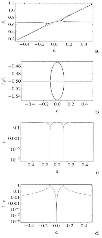
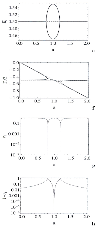
Figure 1: Energies $E_{i}$ (full lines) (a,e), widths $\Gamma_{i}/2$ (b,f), phase rigidity $r_{1}=r_{2}$ (c,g), and $1-r_{k}$ (d,h) of the two eigenfunctions of ${\cal H}^{(2)}$ as a function of the distance $d$ between the two unperturbed energies $e_{1}$ and $e_{2}$. The parameters are given, respectively, in the first and second row of Tab. 1. The dashed lines in (a,e) and (b,f) show, respectively, the $e_{i}$ and $\gamma_{i}/2$ trajectories.

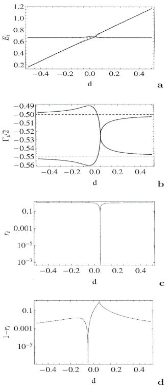
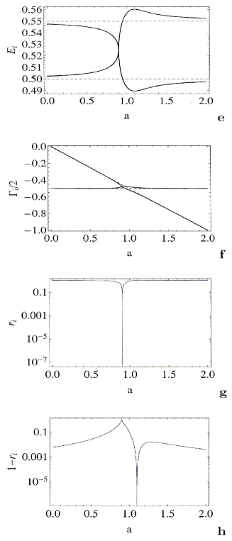
Figure 2: The same as Fig. 1 but with the parameters given, respectively, in the third and fourth row of Tab. 1.

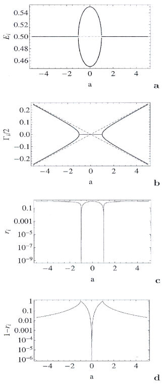
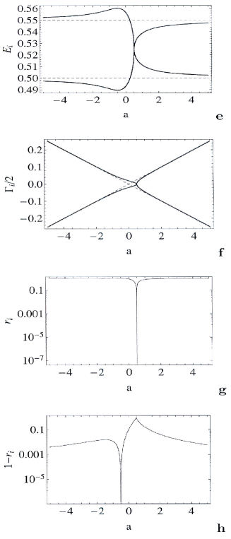
Figure 3: The same as Fig. 1 but with the parameters given, respectively, in the fifth and sixth row of Tab. 1.

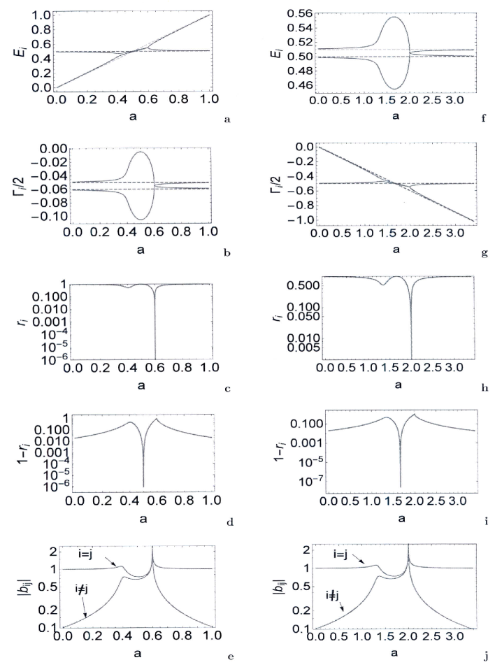
Figure 4: The same as Fig. 1 but with the parameters given, respectively, in the seventh and eighth row of Tab. 1. In (e) and (j), the mixing coefficients $|b_{ij}|$ of the wavefunctions, defined by (15), are shown.

Results for examples with two EPs according to Eqs. (18) to (20) and (21) to (23), respectively, are shown in Fig. 1. The numerical results agree with the analytical ones : the phase rigidity approaches zero at the two EPs; while in between the EPs, we see width bifurcation in the first case (Fig. 1.b) and level repulsion in the second case (Fig. 1.e). The result $r_{k}\to 0$ at every EP corresponds to the expectation of theory top . However, there is an unexpected sharp transition to $r_{k}\to 1$ at the point of maximum width bifurcation or maximum level repulsion. This means that here the two eigenfunctions of ${\cal H}^{(2)}$ are (almost) orthogonal to one another. Far from the critical region, the phase rigidity approaches the value $1$ according to the fact that the influence of the environment onto the system can be neglected, to a good approximation, far from EPs.

The results for the more realistic case with complex coupling strength $\omega$ are shown in Fig. 2. Here, only one EP appears. In a finite parameter distance from the EP, we see maximum width bifurcation (Fig. 2.b) and maximum level repulsion (Fig. 2.e), respectively. Again, $r_{k}\to 0$ at the EP and $r_{k}\to 1$ at maximum width bifurcation or maximum level repulsion.

The results in Fig. 3 show the eigenvalue and phase rigidity pictures for the case when not only loss (as in Figs. 1 and 2) appears but also gain is a possible process. Fig. 3 left panel shows the case with balanced loss and gain, corresponding to $\Gamma_{k}=0$ in the finite parameter range between the two EPs (see Fig. 3.b). Formally, this case is similar to those discussed recently in many papers related to non-Hermitian operators with $PT$ symmetry whose eigenvalues are real in a finite parameter range, see e.g. bender ; bender2 . The $PT$-symmetry breaking is caused by EPs.

The results shown in Fig. 3 left panel have the same characteristic features as those shown in Fig. 1 right panel. The same holds true when the coupling strength $\omega$ is complex (Fig. 3 right panel as compared to Fig. 2 right panel).

In Fig. 4, some results are shown with, respectively, almost imaginary (left panel) and almost real (right panel) coupling strength $\omega$. We see again the characteristic sharp transition $r_{k}\to 0$ in approaching the EP and $r_{k}\to 1$ at another parameter value at which we have maximum width bifurcation and maximum level repulsion, respectively. Additionally, we show in Fig. 4 the mixing of the wavefunctions expressed by the coefficients $|b_{kl}|$ which are defined in (15). At the EP, $|b_{kl}|\to\infty$ as shown in top . As in the other figures with complex coupling strength $\omega$ (Figs. 2 and 3 right panel), there is only one EP. The point of maximum width bifurcation and maximum level repulsion, respectively, appears at a finite parameter distance from the EP. In this parameter region, the two wavefunctions are strongly mixed. The mixing remains when $r_{k}\to 1$ is approached. Beyond $r_{k}\to 1$, we see the hint to a nearby EP ($0<r_{k}<1$) which limits the extension of the total critical parameter region. Beyond this critical parameter region, the wavefunctions approach their original orthogonal character. The physical meaning of the mixing of the wavefunctions under the influence of EPs is discussed in detail in nearby1 ; nearby2 . Here, we underline only that the wavefunctions are mixed when $r_{k}\to 1$, i.e. when they are almost orthogonal in the critical parameter region.

V.2 $N>2$ states

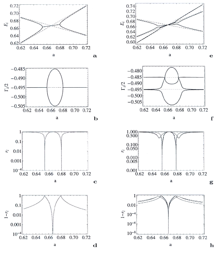
Figure 5: Energies $E_{i}$ (full lines) (a,e), widths $\Gamma_{i}/2$ (b,f), phase rigidity $r_{i}$ (c,g), and $1-r_{i}$ (d,h) of the two eigenfunctions of ${\cal H}^{(2)}$ (left panel) and of the three eigenfunctions of ${\cal H}^{(3)}$ (right panel), respectively, as a function of the parameter $a$. The dashed lines in (a,e) and (b,f) show, respectively, the $e_{i}$ and $\gamma_{i}/2$ trajectories. The parameters are $\omega=0.01\,i$;  $e_{1}=1-1/2~{}a;~{}~{}e_{2}=a$;   $e_{3}=-1/3+3/2~{}a$ (e-h);   $\gamma_{1}/2=\gamma_{2}/2=-0.495$;   $\gamma_{3}/2=-0.4853$ (e-h).

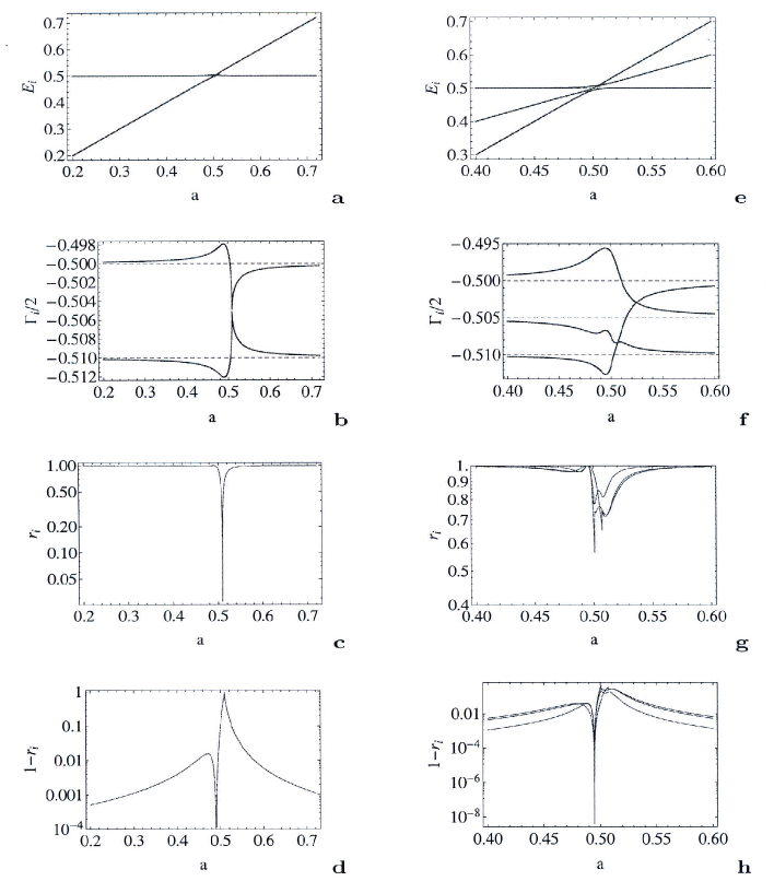
Figure 6: The same as Fig. 5 but $\omega=0.005(1+i)$ and $~{}~{}\gamma_{1}/2=-0.5;~{}~{}\gamma_{2}/2=-0.51;~{}~{}e_{1}=0.5;~{}~{}e_{2}=a$ (left panel) and $~{}~{}\gamma_{1}/2=-0.5;~{}~{}\gamma_{2}/2=-0.505;~{}~{}\gamma_{3}/2=-0.51;~{}~{}e_{1}=0.5;~{}~{}e_{2}=a;~{}~{}e_{3}=2a-0.5$ (right panel).

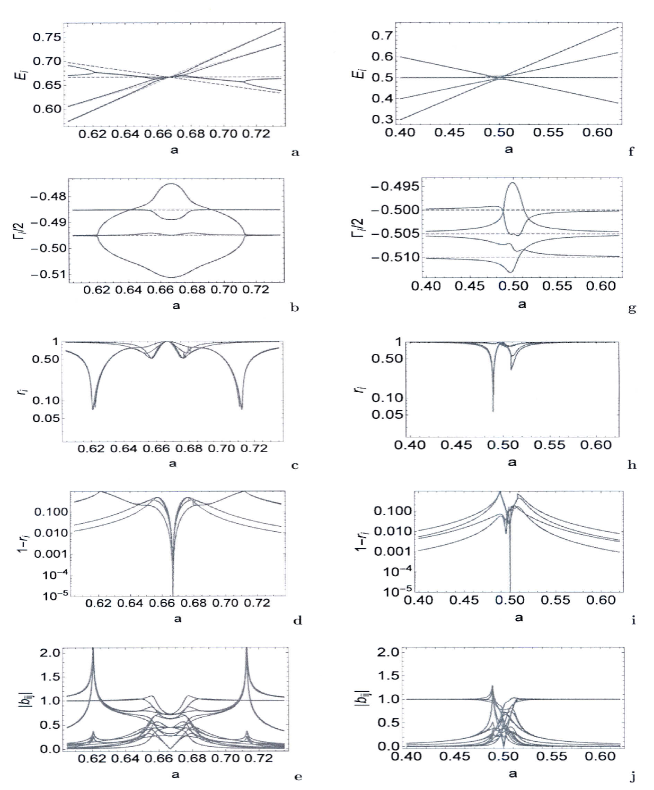
Figure 7: Energies $E_{i}$ (full lines) (a,f), widths $\Gamma_{i}/2$ (b,g), phase rigidity $r_{i}$ (c,h), $1-r_{i}$ (d,i), and mixing coefficients $|b_{ij}|$ of the wavefunctions, defined by (15), of the four eigenfunctions of ${\cal H}^{(4)}$ as a function of the parameter $a$. The dashed lines in (f,g) show, respectively, the $e_{i}$ and $\gamma_{i}/2$ trajectories. The parameters are $\omega=0.01\,i$;   $e_{1}=1-a/2;~{}~{}e_{2}=a;~{}~{}e_{3}=-1/3+3/2~{}a;~{}~{}e_{4}=2/3;~{}~{}\gamma_{1}/2=\gamma_{2}/2=-0.4950;~{}~{}\gamma_{3}/2=-0.4853;~{}~{}\gamma_{4}/2=-0.4950$   (left panel) and $\omega=0.005\,(1+i)$;   $e_{1}=0.5;~{}~{}e_{2}=a;~{}~{}e_{3}=2a-0.5;~{}~{}e_{4}=1-a;~{}~{}\gamma_{1}/2=-0.5;~{}~{}\gamma_{2}/2=-0.505;~{}~{}\gamma_{3}/2=-0.51;~{}~{}\gamma_{4}/2=-0.505$   (right panel).

In Fig. 5, we show the influence of a ”third” state onto the eigenvalue picture and the phase rigidity around an EP in a system that is symmetric around the crossing point of the $e_{i}$ trajectories. New EPs can be identified in the three-level case in the eigenvalue pictures and, correspondingly, in the values of the phase rigidity ($r_{i}<1$). The two EPs near to the crossing point of the $e_{i}$ trajectories are well expressed, and we see clear hints to the existence of two other distant EPs. Most interesting result is the sharp transition from a reduced value $r_{i}<1$ of the phase rigidity (which is characteristic of an EP in the neighborhood) back to $r_{i}\to 1$ at maximum width bifurcation. This abrupt transition occurs in both, the two-level system and the three-level one. At this parameter value, the eigenfunctions of the non-Hermitian Hamiltonian ${\cal H}^{(2)}$ as well as those of ${\cal H}^{(3)}$ become almost orthogonal. At and around this critical parameter value, the wavefunctions of the states are strongly mixed in both, the two-level case and the three-level case nearby2 .

Fig. 6 shows results for a more realistic case with complex coupling strength $\omega$ between system and environment. In the three-level case, hints to the existence of different (distant) EPs can be seen. The sharp transition $r_{i}\to 1$ at maximum width bifurcation however appears very clearly not only in the two-level case but also in the three-level case.

The results shown in the Figs. 5 and 6 characterize the generic behavior of many-level open quantum systems under the condition that the width bifurcation is maximum. The results are confirmed by those which we received in many other calculations performed with different parameters (including for systems which allow loss and gain); or with a larger number $N$ of states. For illustration we show numerical results obtained for $N=4$ states in Fig. 7. Again we see hints to several EPs as well as the sharp transition of $r_{i}$ to a value almost 1 at a critical parameter value. Here, the wavefunctions of all four states are strongly mixed.

VI Discussion of the results

VI.1 $N=2$ states

Most surprising result of our study is the strong parameter dependence of $r_{k}$ in a certain critical region around an EP. The variation $r_{k}\to 0$ in approaching an EP is expected from Eq. (8). The rapid variation $r_{k}\to 1$ when, respectively, the maximum width bifurcation and level repulsion is approached, is however unexpected. The width bifurcation or level repulsion starts at the EP without any enhancement of the coupling strength between system and environment. It is driven exclusively by the nonlinear source term of the Schrödinger equation (14) which describes the open quantum system. When $r_{k}\to 1$ the wavefunctions of the two states, the eigenfunctions of which coalesce (up to a phase factor) at the EP (correspondingly to $r_{k}\to 0$), become almost orthogonal to one another. The transition from $r_{k}\to 0$ (at the EP) to $r_{k}\to 1$ (where width bifurcation and level repulsion, respectively, is maximum) occurs suddenly as function of the varied parameter in all our calculations. The wavefunctions of the two states behave smoothly, i.e. they remain mixed also when $r_{k}\to 1$.

The physical meaning of this result consists in the fact that a stabilization of the localized part of the system occurs when the interaction $\omega$ between system and environment is strong enough, i.e. when it is of the same order of magnitude as the widths $\gamma_{i}/2$. Then, in the case of Eqs. (18) to (20), one of the two states receives a very short lifetime due to width bifurcation, and becomes almost indistinguishable from the states of the environment. Although this process seems to be reversible according to the figures for the eigenvalues, this is in reality not the case. The processes occurring in approaching $r_{k}\to 1$, take place, as mentioned above, by means of the nonlinear source term of the Schrödinger equation near an EP. Due to these processes, the long-lived state has “lost” its short-lived partner with the consequence that the two original states cannot be reproduced. This evolution is therefore irreversible. The long-lived state is more stable than the original one, and the system as a whole (which has lost one state) is more stable than originally. The wavefunction of this long-lived state is mixed in those of the original states.

The stabilization of the system due to Eqs. (21) to (23) occurs in an analog manner. Due to level repulsion, the two states separate from one another in energy, such that their interaction with one another is, eventually, of the same type as that with all the other distant states of the system. That means, each of the original states has “lost” its partner, also in this case; and the reproduction of the two originally neighbored states is prevented. As a result, the interaction of the states of the system via the environment is reduced (since all states are distant in energy), with the consequence that the system can be described well as a closed (almost stable) system. In difference to the case with width bifurcation, however, the number of states of the system as a whole remains unchanged.

Eqs. (18) to (23) with purely imaginary and real coupling strength $\omega$, respectively, will seldom be realized. They allow us however to receive analytical results (see Sect. II) and to understand the basic mechanism. Our numerical results for the more realistic cases with complex $\omega$ show the same effects. The interesting critical parameter range is that between the position of the EP and that of the maximum width bifurcation or level repulsion, respectively, as shown in the figures with complex $\omega$. In this parameter range, the wavefunctions are strongly mixed and $r_{k}$ varies suddenly from the value 0 at the EP, according to (8), to the value almost 1, characteristic for almost orthogonal states at maximum width bifurcation and level repulsion, respectively. When $r_{k}\to 1$, the wavefunctions remain strongly mixed in relation to the original ones in all cases.

The results are very robust and show the same characteristic features in all cases studied by us. They hold true for systems with loss (corresponding to decaying systems) and also for those in which gain may occur (by absorbing particles from the environment). They hold true also when gain and loss are balanced.

It should be underlined here once more that a quantum system is really open and its properties are strongly influenced by the environment of scattering wavefunctions only in the vicinity of EPs. Here, neighboring states may strongly interact via the environment and may cause some decoupling of the whole system from the environment, as shown above. As a result of this decoupling, the system is stabilized; behaves “linearly”; and Fermi’s golden rule is applicable.

The eigenvalues shown in Fig. 3 left panel are real in the parameter range between the two EPs. This might be interpreted as a signature of $PT$-symmetry. The Hamiltonian ${\cal H}^{(2)}$ is non-Hermitian also in this parameter range. The wavefunctions are biorthogonal and the phase rigidity is different from 1 for all parameter values including those for which the eigenvalues are real. The corresponding $r_{i}$ are near to 1, and not equal to 1. All calculations in this parameter range for realistic systems can therefore be performed, to a good approximation, by using a Hermitian Hamiltonian. Nevertheless, such a calculation for an open quantum system remains an approximation, although it will provide good results.

Moreover, the parameters used in Fig. 3 left panel are unrealistic for a physical system. The coupling parameter $\omega$ is usually complex as discussed in, e.g., top ; nearby1 . The eigenvalues obtained in a corresponding calculation are no longer real in a certain finite parameter range, see the example Fig. 3 right panel. Also in this case, PT symmetry breaking may appear and the behavior of the system at maximum width bifurcation is determined by the nonlinear source term involved in the Schrödinger equation for an open quantum system; and we have the jump-like transition $r_{i}\to 1$ at maximum width bifurcation also in this less symmetric case.

The phenomenon of almost orthogonal wavefunctions at maximum width bifurcation (or maximum level repulsion) is robust as Figs. 1 to 4 for different two-state systems show. It is not an artifact of the two-state model (3) since it appears also in calculations with more than two states (see Sect. V.2).

VI.2 $N>2$ states

All our calculations with $N>2$ states are performed in the parameter region in which a higher-order EP is expected. Signatures of the existence of such a higher-order EP are not found in any of the results. This is, of course, not astonishing since every EP is a point in the continuum and therefore of measure zero. Also the second-order EPs (crossing points of two eigenvalue trajectories) can be identified only by their influence onto observables in their neighborhood. Our results show clearly that this holds true also for higher-order EPs.

One of the characteristic features of an EP (i.e. of the crossing point of two eigenvalue trajectories) is that the two eigenfunctions in its surrounding are mixed due to the coupling of the system to a common environment nearby1 . This environmentally-induced interaction of the states is large at and near to an EP (where the phase rigidity of the wavefunctions is reduced, as discussed in Sect. II). A nearby state does therefore not interact with the original states which cross at the EP. It interacts rather with some states, the wavefunctions of which are mixed in those of the original states (according to (15)). At and near to these crossing points, new EPs of second order appear, the ranges of influence of which overlap. In other words, a clustering of EPs occurs, see the discussion in section IV.

It is this phenomenon of clustering of EPs which we see in Figs. 5 to 7. It occurs in the parameter range of a higher-order EP. The results are generic and provide us valuable information on the dynamics of open quantum systems. Most interesting is the phenomenon of the jump-like enhancement of the phase rigidity when the maximum width bifurcation is parametrically approached. This effect is of the same type as that observed numerically for two states and discussed in detail in Sects. V.1 and VI.1, respectively.

VII Conclusions

In this paper we have described open quantum systems by means of a Schrödinger equation the Hamiltonian ${\cal H}$ of which is completely non-Hermitian. It contains explicitly (in the non-diagonal matrix elements) the interaction of the states via the environment. The eigenvalues of ${\cal H}$ are complex and the eigenfunctions are biorthogonal. Most interesting property is that the eigenvalues of two states may coalesce in one point (the so-called EP), at which also the corresponding eigenfunctions are the same, up to a phase top . The EPs are singular points and play an important role for the dynamics of open quantum systems.

We used also the equivalent description of the system by means of a Schrödinger equation with the non-Hermitian Hamilton operator ${\cal H}_{0}$ (with vanishing non-diagonal matrix elements) and source term. Here, the interaction of the states via the environment is contained in the source term, and not in the Hamiltonian. The source term is nonlinear near and at EPs. It drives the behavior of the open quantum system and determines the dynamics of open quantum systems.

Our main concern of the present paper is the phase rigidity $r_{i}$ of the eigenfunction $\Phi_{i}$ of ${\cal H}$. This value provides a quantitative measure for the biorthogonality of the wavefunction of the state $i$, i.e. for the possibility to influence the properties of the system by the environment. It holds $1\geq r_{i}\geq 0$. At $r_{i}\approx 1$, the wavefunctions are almost orthogonal, very much like the eigenfunctions of a Hermitian operator. For vanishing $r_{i}$ however, the eigenfunctions of the non-Hermitian operator are really biorthogonal, and the influence of the environment is extremely large. This influence may cause, among others, a mixing of the wavefunctions of the different states via the environment. In nearby1 ; nearby2 , the modification of the eigenfunction $\Phi_{i}$ of the non-Hermitian Hamilton operator ${\cal H}$ due to its coupling to other states of the system via the environment is studied in detail. The resulting mixing of the wavefunctions can be expressed by the relation (15). At and near to an EP, the mixing is extremely large.

We studied first the phase rigidity in a two-level system around an EP. In all our calculations, the coupling strength $\omega$ between system and environment is fixed. Only the energies $e_{i}$ or widths $\gamma_{i}$ of the states are parametrically varied. We have $r_{i}\approx 1$ far from an EP and $r_{i}\to 0$ in approaching an EP. This result is expected from analytical studies.

We observe however also another result in the critical region around an EP which is completely unexpected. In approaching the maximum width bifurcation and level repulsion, respectively, the value of the phase rigidity varies rapidly from its value $r_{i}<1$ to $r_{i}\approx 1$. That means, that the two wavefunctions are almost orthogonal when the width bifurcation or level repulsion is maximum. This jump-like variation of the phase rigidity is observed at fixed coupling strength between system and environment. It is caused therefore exclusively by the nonlinear source term of the Schrödinger equation. The wavefunctions of the states remain mixed at this critical parameter value, although they are almost orthogonal according to $r_{i}\to 1$.

This phenomenon occurs not only in the simple two-state model (see Sect. V.1) but also in the case with more than two states (see Sect. V.2). In the first case, we have well separated EPs while there is some clustering of EPs in the second case. That means, the clustering of EPs does not destroy the effect, see Figs. 5 to 7. Quite the contrary, the clustering of many EPs causes a dynamical phase transition from an open quantum system (with biorthogonal eigenfunctions of its states) to an almost closed system (with almost orthogonal eigenfunctions of its states). The underlying process is irreversible and causes a stabilization of the whole system, meaning that the open system can be described approximately as a closed system. The wavefunctions at both sides of the dynamical phase transition are non-analytically related to one another and differ fundamentally from one another. This feature is characteristic of any phase transition. The wavefunctions of the states on one side of the phase transition might be obtained by using the two-body residual forces derived from forces between free particles. This will be impossible, however, on the other side of the transition where the wavefunctions are modified due to the mixing of the different states of the system via the common environment.

Our results provide the following generic feature of open quantum systems. When two states are near to one another in energy or in lifetime, they may strongly interact with one another via the continuum of scattering wavefunctions due to the existence of a singular point (EP) in their vicinity. Here, the Schrödinger equation contains non-linear terms; irreversible processes occur; and the whole system will be stabilized. As a result, the system behaves very much like a closed system that is localized in space : The eigenstates are almost orthogonal and the eigenvalues are almost real (and sometimes even completely real top ). Such a situation can be described well by a Hermitian operator where the lifetime of a state does not appear explicitly. By this, the meaning of lifetime for the characterization of the individual states of the system is lost. Characteristic of the states are solely their energies and wavefunctions, while the lifetimes can be obtained by using perturbation methods.

Nevertheless, the results presented in our paper show that energy and time are related to one another in quantum mechanical systems. It is shown in [15] that time is bounded from below in non-Hermitian quantum physics. This follows from the fact that the decay widths (inverse proportional to the lifetimes of the states) cannot increase limitless. Thus, time is bounded from below in the same manner as energy, in contrast to the assumptions of Hermitian quantum physics. Pauli has used this argument of Hermitian quantum physics, see e.g. [23], in order to conclude that the uncertainty relation between time and energy can, on principle, not be derived, for details see e.g. fdp1 . The uncertainty relation between energy and time remained therefore a puzzling phenomenon in Hermitian quantum physics. As our results show, this phenomenon is not at all puzzling in non-Hermitian quantum physics.

Concluding, we recall the phenomenon of resonance trapping top observed many years ago. Resonance trapping occurring in an open quantum system coupled strongly to the environment, prevents the overlapping of individual resonance states. Consequently, the system is practically always in the regime of weakly (or not) overlapping resonances, see e.g. top ; harney . In analogy to this phenomenon, an open quantum system can be described quite well by a Hermitian Hamiltonian on both sides of the dynamical phase transition. This statement agrees completely with experience. Interesting non-trivial features of open quantum systems appear only in the parameter range in which a clustering of EPs and therewith a dynamical phase transition occurs. One of many examples is the relation between reduced phase rigidity and enhanced transmission through a quantum dot burosa .

The results presented in this paper are generic. We believe that they will initialize further studies for concrete systems under concrete conditions. By this, they will provide new interesting results for open quantum systems, especially in the parameter range of a dynamical phase transition.

References

- (1) I. Rotter and J.P. Bird, A Review of Progress in the Physics of Open Quantum Systems: Theory and Experiment, Rep. Progr. Phys. 78, 114001 (2015)
- (2) I. Rotter, J. Phys. A 42, 153001 (2009)
- (3) T. Kato, Perturbation Theory for Linear Operators, Springer, Berlin 1966
-
(4)
E. Hernandez, A. Jauregui, and A. Mondragon,
J. Phys. A 39, 10087 (2006);
E. Hernandez, A. Jauregui, A. Mondragon, and L. Nellen, Intern. Journ. Theoretical Physics 46, 1666 (2007) and 46, 1890 (2007);
E. Hernandez, A. Jauregui, and A. Mondragon, Phys. Rev. E 84, 046209 (2011) -
(5)
G.A. Álvarez, E.P. Danieli, P.R. Levstein and
H.M. Pastawski, J. Chem. Phys. 124, 194507 (2006);
H.M. Pastawski, Physica B 398, 278 (2007) -
(6)
E. Narevicius, P. Serra, and N. Moiseyev,
Europhys. Lett. 62, 789 (2003) ;
R. Uzdin, A. Mailybaev, and N. Moiseyev, J. Phys. A 44, 435302 (2011) -
(7)
A. Jaouadi, M. Desouter-Lecomte, R. Lefebvre, O. Atabek,
Journ. Phys. B 46, 145402 (2013);
A. Jaouadi, M. Desouter-Lecomte, R. Lefebvre, and O. Atabek, Special Issue Quantum Physics with Non-Hermitian Operators: Theory and Experiment, Fortschr. Phys. 61, 162 (2013);
R. Lefebvre, O. Atabek, Chem. Phys. 399, 111 (2012);
O. Atabek, R. Lefebvre, M. Lepers, A. Jaouadi, O. Dulieu, V. Kokoouline, Phys. Rev. Lett. 106, 173002 (2011) - (8) A. Leclerc, G. Jolicard, and J.P. Killingbeck, J. Phys. B 46, 145503 (2013)
- (9) N. Moiseyev, Non-Hermitian Quantum Mechanics, Cambridge University Press (2011)
- (10) C. Jung, M. Müller, and I. Rotter, Phys. Rev. E 60, 114 (1999)
- (11) W.D. Heiss, M. Müller, and I. Rotter, Phys. Rev. E 58, 2894 (1998)
- (12) H. Eleuch and I. Rotter, Eur. Phys. J. D 69, 230 (2015)
- (13) H. Eleuch and I. Rotter, Eur. Phys. J. D 69, 229 (2015)
- (14) Y.V. Fyodorov and D.V. Savin, Phys. Rev. Lett. 108, 184101 (2012)
- (15) J.B. Gros, U. Kuhl, O. Legrand, F. Mortessagne, E. Richalot, and D.V. Savin, Phys. Rev. Lett. 113, 224101 (2014)
- (16) In contrast to the definition that is used in, for example, nuclear physics, we define the complex energies before and after diagonalization of by and , respectively, with and for decaying states. This definition will be useful when discussing systems with gain (positive widths) and loss (negative widths), see, e.g., top ; nearby1 .
- (17) I. Rotter, Special Issue Quantum Physics with Non-Hermitian Operators: Theory and Experiment, Fortschr. Phys. 61, 178 (2013)
- (18) B. Wahlstrand, I.I. Yakimenko, and K.F. Berggren, Phys. Rev. E 89, 062910 (2014)
- (19) In studies by some other researchers, the factor in (8) does not appear. This difference is discussed in detail and compared with experimental data in the Appendix of fdp1 and in Sect. 2.5 of top , see also Figs. 4 and 5 in berggren .
- (20) I. Rotter, Phys. Rev. E 64, 036213 (2001)
-
(21)
L. Landau, Physics Soviet Union 2, 46 (1932);
C. Zener, Proc. Royal Soc. London, Series A 137, 692 (1932) - (22) J.P. Jeukenne and C. Mahaux, Nucl. Phys. A 136, 49 (1969)
- (23) C.M. Bender, Rep. Progr. Phys. 70, 947 (2007)
- (24) C.M. Bender, M. Gianfreda, S.K. Özdemir, B. Peng, and L. Yang, Phys. Rev. A 88, 062111 (2013)
- (25) W. Pauli, Handbuch der Physik: Encyclopaedia of Physics (edited by S. Flügge), Vol. 5/1, p. 60, Springer Berlin 1958
- (26) F.M. Dittes, H.L. Harney and I. Rotter, Phys. Lett. A 153, 451 (1991)
-
(27)
E. N. Bulgakov, I. Rotter, and A. F. Sadreev,
Phys. Rev. E 74, 056204 (2006) and
Phys. Rev. B 76, 214302 (2007)