Ten Kepler eclipsing binaries containing the third components.

Abstract

Analyzing the available photometry from the Kepler satellite and other databases, we performed the detailed light curve modelling of ten eclipsing binary systems, which were found to exhibit a periodic modulation of their orbital periods. All of the selected systems are detached ones of Algol-type, having the orbital periods from 0.9 to 2.9 days. In total, 9448 times of minima for these binaries were analysed, trying to identify the period variations caused by the third bodies in these systems. The well-known method of the light-travel time effect was used for the analysis. The orbital periods of the outer bodies were found to be between 1 and 14 years. This hypothesis makes such systems interesting for a future prospective detection of these components, despite their low predicted masses. Considering the dynamical interaction between the orbits, the most interesting seems to be the system KIC 3440230, where one would expect detection of some effects (i.e. changing the inclination) even after a few years or decades of observations.

1. Introduction

The eclipsing binaries (EBs) provide us with an excellent method how to derive the basic physical properties of the two eclipsing components (their radii, masses, temperatures). Moreover, they can also serve as independent distance indicators, one can study the dynamical evolution of the orbits, test the stellar structure models, or discover additional components in these systems (see e.g. Guinan & Engle 2006). On the other hand, the Kepler satellite (Borucki et al., 2010) provides us with unprecedented accuracy of photometric data. From this huge set of observations, 1879 eclipsing binaries were detected after the first data release (Prša et al., 2011), later extended to 2165 (Slawson et al., 2011).

Such a huge database of eclipsing binaries observed with superb precision and monitored continuously over a period of four years encouraged several teams for looking for a periodic modulation of data, indicating the triple systems. The use of such method and its limitations were described elsewhere (e.g. Irwin 1959, or Mayer 1990). For example Gies et al. (2012) presented 41 suspected triples, while Conroy et al. (2014) listed 236 potential triples. More is also promised to be published by J.A.Orosz (see Conroy et al. 2014), but it was not published yet. Moreover, Rappaport et al. (2013) presented 39 dynamically interesting systems, where the third-body periods are short enough (if compared with the binary period), hence some interaction between the orbits is expected or even observed (e.g. changing of the inclination). On the other hand, most of the triples listed in Conroy et al. (2014) have periods of the order of hundreds or even thousands of days. So long periods were usually only estimated (due to limited coverage of the Kepler data), or are influenced by large errors.

From this reason, we decided to perform a similar analysis of detecting the third-body signals for some other systems, but based on a larger data set, if available. For some of the systems, we tried to observe additional ground-based observations. These were done quite recently, hence even a single point can help us to better constrain the third-body period. And finally, we also tried to find some photometry from other sources, like the survey data from SuperWASP (Pollacco et al., 2006), NSVS (Woźniak et al., 2004), ASAS (Pojmanski, 2002), and others. These (mostly rather scattered) points help us to prove a long-term stability of the orbital period of the close pair, or its evolution (e.g. the quadratic ephemeris).

2. Selection process for the binaries

All the studied systems were chosen according to their remarkable variations in the $O-C$ diagrams. Such ten systems naturally complete a set of triple systems as presented by Gies et al. (2012) and Conroy et al. (2014). However, these two published studies presented only such binaries, in which the third body variations are visible on the Kepler data set, and the ones with longer periodic modulation were omitted or only briefly mentioned. This is the main impact of the present paper. We decided to study also these systems, where the orbital periods of the third bodies are longer and we harvested for such an analysis also the ground-based surveys and our new photometric data. Obviously, this also leads to the conclusion that the multiplicity fraction should be even higher than resulted from the previous studies, because a non-negligible number of triples has the third-body orbital period of the order of years, decades, or even longer.

For the systems under our analysis we have chosen only such systems which fulfill the following criteria: \footnotesize1⃝ All of them are Algol-type detached binaries with circular orbits. This information was taken from the visual inspection of the Kepler eclipsing binary catalogue. \footnotesize2⃝ All have remarkable curvatures in their $O-C$ diagrams, which was considered on the basis of Gies et al. (2012) and Conroy et al. (2014) minima times plotted into the $O-C$ diagrams in the $O-C$ gateway (Paschke & Brát, 2006). \footnotesize3⃝ None of these systems was studied before concerning the third-body orbits (only a brief remark in Gies et al. (2012) with no orbital solution is not counted for). \footnotesize4⃝ For each of them also some additional photometry exists (older or a more recent one) besides the Kepler data. At this point it is worth to mention that two of the analysed systems (KIC 7630658, and KIC 9007918) were not included in the previous work on Kepler triples detected by eclipse timing by Gies et al. (2012). Therefore, we have to emphasize that due to these rather limited selection mechanisms our study does not aim to present a complete sample for any statistical analysis of Kepler EBs. As a by-product some systems were found to exhibit no visible variation or yielded rather spurious results yet, see below.

3. Photometry and light curve modelling

The analysis of the light curves (hereafter LC) based on the Kepler photometry was carried out using the program PHOEBE (Prša & Zwitter, 2005) for all of the systems. This program is based on the Wilson-Devinney algorithm (Wilson & Devinney, 1971) and its later modifications. However, some of the parameters have to be fixed during the fitting process. The limb darkening coefficients were interpolated from the van Hamme s tables (van Hamme, 1993). The albedo coefficients $A_{i}$, the gravity darkening coefficients $g_{i}$, and also the synchronicity parameters $F_{i}$ were also computed during the fitting process due to the high quality of the photometry. The same apply for the value of the third light, which was also considered as a free parameters and has been fitted (in agreement with our third-body hypothesis). The temperature of the primary component was kept fixed according to the $T_{1}$ value as given in the Kepler catalogue (Brown et al., 2011), while only the secondary temperature was fitted. In our final solution we only present a ratio of the temperatures $T_{2}/T_{1}$ for a higher robustness due to (sometimes) problematic values of the $T_{1}$ from the Kepler catalogue. An issue of the mass ratio was solved by fixing $q=1$ because no spectroscopy for these selected systems exists, and for detached eclipsing binaries the LC solution is almost insensitive to the photometric mass ratio (see e.g. Terrell & Wilson 2005).

The quality of the LC fit is even noticeable by a naked eye, see Fig. 1. The automatic routines as used e.g. by Slawson et al. (2011) are definitely better for reduction of a huge data sets of hundreds of binaries, however the codes sometimes produce spurious results. If we analyse the particular system in more detail, we are able to get a better fit to the data, lower residuals, and hence also parameters with lower errors. The automatic pipelines maybe even not compute parameters like albedos, gravity brightening, third light, etc. All of these parameters can be also fitted with the Kepler data and help us to obtain a better fit to the data.

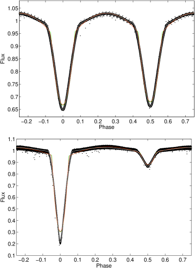
Figure 1.— Illustrative example of the light curves of KIC 09402652 (upper plot), and KIC 10581918 (lower plot) together with their respective fits – from Slawson et al. (2011) plotted in red and green, and our new fit plotted in white.

However, it is necessary to admit that some of the parameters can correlate with each other during the fitting process (this especially apply e.g. for luminosity and temperature, inclination and the third light for partially eclipsing systems, etc). This problem was avoided checking whether there is some value in the correlation matrix higher than 0.8 and such a fit was not accepted. Another iteration with different parameter set was used and this way all the systems were analysed yielding the results presented below.

4. The times of minimum light

The CCD follow-up observations of selected Kepler targets were mostly carried out in Ondřejov Observatory in the Czech Republic (labelled as OND in the tables with minima times), few new observations were also obtained remotely with the BOOTES-1A and BOOTES-2 telescopes located in Spain (labelled as BOO-1, and BOO-2 in the tables with minima times). The new times of primary and secondary minima and their respective errors were determined by the classical Kwee & van Woerden (1956) method or by our new approach (see below). All the times of minima used for the analysis are given in the appendix Tables 5.

For the analysis of minima times and variation of orbital period caused by the third body one needs the minima times as precise as possible. For some of the Kepler targets the times of minima exist and were even published several times, see e.g. Gies et al. (2012), or Conroy et al. (2014). However, their published times of minima differ significantly – sometimes more than their respective errors. One possible explanation is that the above-mentioned teams included and not included an error in barycentric times of the Kepler data, which was first mentioned in ”Kepler Data Release 19”.

Due to this reason, we have proceeded in the following way. At first, the times of minima published by Gies et al. (2012) were taken and plotted into the $O-C$ diagram. The same was done with the data by Conroy et al. (2014) and the $O-C$ diagrams were analysed whether some periodic modulation due to the third body is presented. Then, the original data from the Kepler archive were downloaded and analysed. Such an analysis was done in several steps. At first, from the original raw fits files the photometry was extracted, the flux converted into magnitudes and the individual light curves in different quarters of data were analysed and the theoretical light curves were constructed. Lets call this way the Method 1. On the other hand, the Method 2 was using the data downloaded from the EB catalogue by Slawson et al. (2011), which were already detrended and the normalised flux versus BJD was provided. These light curves were analysed and used to construct the theoretical light curve (but from the whole Kepler mission).

The theoretical light curves were used to derive the times of minima following the AFP method as described in Zasche et al. (2014). Using the LC templates from Method 1 and 2 and also the times of minima from Gies et al. (2012) and Conroy et al. (2014), we have four different sets of times of minima for the analysis (disadvantage of the Gies et al. (2012) data is the fact that only a portion of the Kepler data was provided, these ones after reducing the first 9 quarters only). These four data sets differ significantly sometimes and the best one (with the lowest scatter) was used for the subsequent analysis of a particular system. Usually, the best one was the data set obtained by Method 2.

However, it is natural that some limitations of the method play a role. The most critical issue is the fact that for deriving the times of minima we always use the same LC template. However, for some cases the shape of the LC varies during the Kepler mission and the difference is sometimes visible even by naked eye (see below comments for particular systems). This problem can be avoided using the different LC templates for data obtained during the different time epochs. However, it is a questionable task whether using five or a hundred different LC templates for the whole Kepler data set would provide a better result. Hence, we solved out this problem by using a slightly different template for each Kepler quarter.

If we compare both minima derivation methods, we found some aspects of the problem. The classical Kwee & van Woerden method was used only for recent observations due to the fact that only small parts of the minima were observed and the whole LC cannot be fitted. On the other hand, the AFP method can provide us with much more precise result even with lower number of observations, but one needs the complete LC template, hence the complete observed LC. Generally, the individual errors from the AFP method are a bit lower (but not 10 times lower) than the classical errors from the Kwee & van Woerden method and are not affected by any observational biasses, wrong reduction, poor conditions, etc. as can be true for the ground-based ones.

5. The period changes

For the analysis of period changes in these binaries, we used a well-known method introduced by Irwin (1959). It resulted in a set of parameters of the third-body orbit: period of the third body $P_{3}$, eccentricity $e$, semi-amplitude of the variation $A$, time of periastron passage $T_{0}$, and the longitude of periastron $\omega$. The input values for the analysis were the ephemerides ($HJD_{0}$, $P$) given by Slawson et al. (2011), while also these ephemerides were recomputed. If necessary, also the quadratic term of the ephemerides was used (attributed to the mass transfer between the components). The solutions presented below were found using Monte Carlo simulations and the simplex algorithm. However, the individual errors of parameters are taken from the code and may be too optimistic for some of the systems.

All the new precise CCD times of minima from the Kepler satellite were used with a weight of 10 in our computation; some of the less precise measurements were weighted by a factor of five, while the poorly covered minima were given a weight of 1. This apply mostly for the minima times derived from other sources of photometry (like ASAS, SuperWASP, etc.), which were derived using the same method as the Kepler ones, but using a different LC template. The weights were used instead of the uncertainties due to the fact that for the older published minima any information about their accuracy is missing.

Because of studying only the period changes due to the third-body orbit, and all of the systems are circular, for most of the systems only the deeper (primary) minimum was used to detect the period changes.

Table 1Relevant information for the analysed systems.

System	Other ID	RA	DE	$KEP_{\rm max}^{A}$	$(J-H)[\mathrm{mag}]^{B}$	$(B-V)[\mathrm{mag}]^{C}$	Sp.TypeC
KIC 2305372	2MASS J19275768+3740219	19h27m57s.7	+37∘40′21′′.9	13${}^{\rm m}\!\!.$82	0.364
KIC 3440230	2MASS J19215310+3831428	19h21m53s.1	+38∘31′42′′.8	13${}^{\rm m}\!\!.$64	0.317
KIC 5513861	TYC 3123-2012-1	18h57m24s.5	+40∘42′52′′.9	11${}^{\rm m}\!\!.$64	0.238	0.448	wF8V
KIC 5621294	2MASS J19285262+4053359	19h28m52s.6	+40∘53′36′′.0	13${}^{\rm m}\!\!.$61	0.143
KIC 7630658	2MASS J19513965+4315224	19h51m39s.6	+43∘15′22′′.3	13${}^{\rm m}\!\!.$89	0.389
KIC 8553788	2MASS J19174291+4438290	19h17m42s.9	+44∘38′29′′.1	12${}^{\rm m}\!\!.$69	0.120	0.537	A7V
KIC 9007918	TYC 3541-2296-1	19h04m02s.0	+45∘21′21′′.7	11${}^{\rm m}\!\!.$66	0.135	0.155	F5IV
KIC 9402652	V2281 Cyg	19h25m06s.9	+45∘56′03′′.1	11${}^{\rm m}\!\!.$82	0.154	0.470	F8V
KIC 10581918	WX Dra	18h52m10s.5	+47∘48′16′′.7	12${}^{\rm m}\!\!.$80	0.186
KIC 10686876	TYC 3562-961-1	19h56m13s.6	+47∘54′33′′.7	11${}^{\rm m}\!\!.$73	(-0.041)	0.204	F0V

Note: [A] - Kepler database, [B] - 2MASS catalogue, Skrutskie et al. (2006), [C] - based on the Tycho catalogue, Pickles & Depagne (2010).

Table 2Light curve parameters for the analysed systems as resulted from the PHOEBE.

System	$T_{2}/T1$	$i$ [deg]	$\Omega_{1}$	$\Omega_{2}$	$L_{1}$ [%]	$L_{2}$ [%]	$L_{3}$ [%]
KIC 2305372	0.6637 (0.0152)	79.92 (0.27)	5.431 (0.035)	4.134 (0.059)	82.70 (0.90)	17.30 (0.80)	0
KIC 3440230	0.6082 (0.0085)	81.63 (0.82)	6.278 (0.692)	5.114 (0.192)	87.02 (0.83)	12.98 (0.47)	0
KIC 5513861	0.9891 (0.0115)	79.37 (0.08)	5.393 (0.012)	5.773 (0.024)	55.10 (0.23)	43.97 (0.27)	0.94 (0.55)
KIC 5621294	0.5620 (0.0096)	72.32 (0.73)	4.182 (0.084)	4.255 (0.106)	82.85 (0.35)	8.86 (3.02)	11.29 (0.99)
KIC 7630658	0.9635 (0.0004)	79.76 (0.02)	7.660 (0.005)	7.646 (0.007)	51.66 (0.02)	43.26 (0.02)	5.07 (0.02)
KIC 8553788	0.6385 (0.0022)	69.72 (0.22)	5.351 (0.025)	5.106 (0.057)	80.15 (0.71)	13.27 (0.15)	6.56 (0.60)
KIC 9007918	0.6289 (0.0008)	72.83 (0.05)	5.479 (0.006)	5.781 (0.016)	79.06 (0.05)	6.36 (0.02)	14.58 (0.05)
KIC 9402652	0.9956 (0.0033)	79.61 (0.07)	4.386 (0.007)	4.357 (0.004)	50.01 (1.68)	49.99 (1.44)	0
KIC 10581918	0.6813 (0.0126)	88.53 (0.42)	5.595 (0.058)	5.751 (0.050)	86.68 (0.67)	13.32 (0.50)	0
KIC 10686876	0.6532 (0.0048)	88.35 (0.06)	6.976 (0.030)	16.290 (0.123)	92.32 (3.41)	2.76 (0.11)	4.92 (3.08)

Table 3The parameters of the third-body orbits for the individual systems.

System	$HJD_{0}$	$P$	$A$	$\omega$	$P_{3}$	$T_{0}$ [HJD]	e	$f(m_{3})$	$P_{3}^{2}/P$
	(2450000+)	[days]	[days]	[deg]	[yr]	(2400000+)		$[M_{\odot}]$	[yr]
KIC 2305372	4965.9539 (8)	1.4047173 (15)	0.0211 (13)	86.9 (4.7)	10.36 (0.16)	54532 (62)	0.625 (66)	0.4543 (18)	27919
KIC 3440230	5687.5150 (3)	2.8811052 (38)	0.00060 (25)	111.3 (17.5)	1.04 (0.13)	55818 (32)	0.264 (98)	0.0010 (1)	137
KIC 5513861	4955.0004 (9)	1.5102096 (10)	0.00831 (73)	27.2 (7.4)	5.94 (0.18)	56347 (139)	0.135 (89)	0.0861 (39)	8540
KIC 5621294	4954.5109 (2)	0.9389102 (3)	0.00024 (5)	133.9 (11.7)	2.70 (0.10)	56124 (28)	0.654 (175)	0.000014 (2)	2843
KIC 7630658	5003.2780 (2)	2.1511554 (4)	0.00393 (3)	145.9 (1.1)	2.53 (0.01)	67358 (17)	0.680 (10)	0.0875 (33)	1085
KIC 8553788	4954.9856 (13)	1.6061776 (17)	0.00802 (114)	237.3 (8.6)	9.09 (0.08)	56430 (59)	0.764 (93)	0.0429 (50)	18787
KIC 9007918	4954.7485 (2)	1.3872066 (2)	0.00048 (4)	94.6 (9.2)	1.30 (0.08)	56721 (14)	0.662 (170)	0.00034 (4)	445
KIC 9402652	4954.2856 (2)	1.0731067 (2)	0.00427 (17)	266.9 (4.9)	4.08 (0.05)	56343 (11)	0.757 (37)	0.0242 (10)	5670
KIC 10581918	2829.3696 (3)	1.8018668 (34)	0.00209 (58)	0.1 (8.3)	14.05 (0.47)	53244 (530)	0.254 (88)	0.00027 (9)	40023
KIC 10686876	4953.9490 (45)	2.6184137 (50)	0.00563 (189)	280.5 (28.4)	6.72 (0.96)	56990 (442)	0.464 (157)	0.0207 (19)	6302

6. The individual systems

In the following section we present the results of our analysis for all of the systems. The whole procedure is described in detail for the first binary, the others are only briefly discussed due to similarity of the analysis with the first one. The Table 1 summarizes basic information about the stars, their cross-identification, magnitudes and photometric indices. As one can see from the $(J-H)$ index, most of the stars are of F and G spectral type.

6.1. KIC 2305372

The first system in our sample is the star KIC 2305372, which was first recognized as a variable by Hatnet (Hartman et al., 2004) and ASAS (Pigulski et al., 2009) surveys in the pre-Kepler era. After then, it was included into the catalogue of eclipsing binaries in the Kepler field (Slawson et al., 2011). The times of minima were published by Gies et al. (2012) and later by Conroy et al. (2014). However, Gies et al. (2012) presented the system as a candidate triple, while Conroy et al. (2014) roughly estimated some period of about 3700 days. No spectral analysis was carried out, hence we can only estimate that it is probably a system of G spectral type (from the $J-H$ photometric index).

The light curve analysis was carried out from the Kepler detrended data, while its parameters are given in Table 2. As one can see, both components are rather different, while no third light was detected during the LC solution. The final LC fit is presented in Fig.2, where is clearly seen a shape of the LC as a classical Algol one. However, the LC shape seems to be slightly asymmetric (see the outside eclipse curvature). This light curve template was also used for deriving the times of minima (using the method as described above). For the period analysis we collected the Hatnet, ASAS, SuperWASP and the Kepler data points and derived more than 800 times of primary minima for this star. One new minimum was also observed by the authors at Ondřejov Observatory in the Czech Republic.

This data set was analysed and the method of Irwin (1959) was used. The results are given in Table 3 and the final fit is plotted also in the Figure 3. In these plots only the new post-Kepler data and the isolated measurements (groups of up to three data points) are plotted with their respective error bars for a better clarity. Plotting the error bars for all the data would diminish the readability of the graphs (however, for some observations their respective error bars are too small and are plotted almost inside the individual dots). We are aware of the fact that only a few points of poor quality define the shape of the third-body variation and its period $P_{3}$ in the $O-C$ diagram. However, the parabolic fit is not able to describe the data in such detail. From the parameters of the third body one is able to compute also the mass function of the third body in the system, which is also given in Table 3. As one can see, its value is rather high, so the third component should be detected also in the LC solution as a third light contribution. However, no such value was detected during the LC fitting. This still remains an open question, however we also have to mention that the shape of the LC varies in time and the LC fit in different quarters of data differs a bit. This can also influence our result and the minima precision, LC modelling and the third light detection. Regrettably, having no information about the masses of the eclipsing components, one cannot easily set a tighter limit to the mass of the predicted third body.

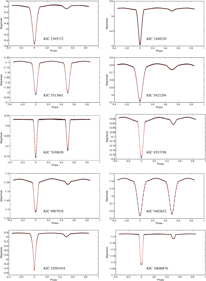
Figure 2.— The Kepler light curves of all studied systems. The red curves present the final fit, the dots stand for the observations.

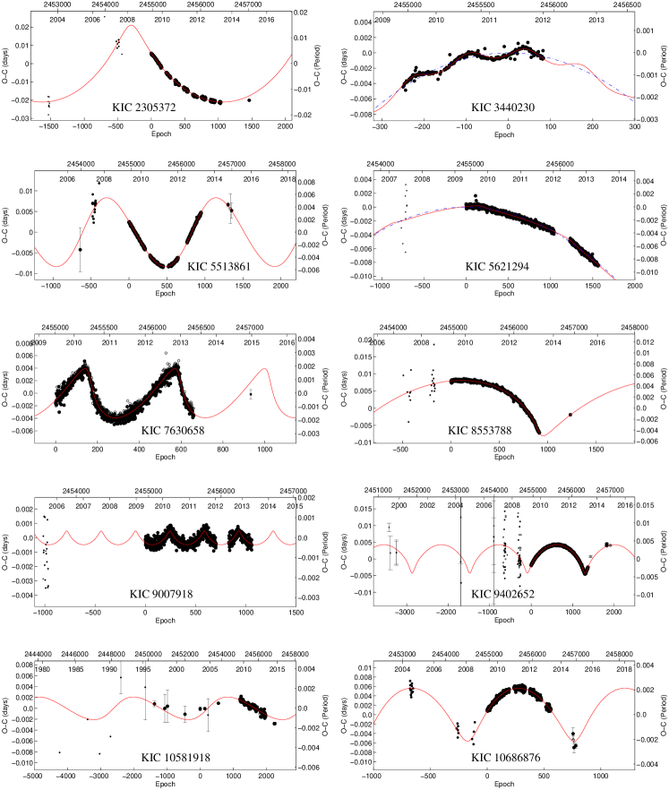
Figure 3.— The $O-C$ diagrams of all studied systems. The red curves present the final fit, the blue dash-dotted curves the quadratic ephemerides. The dots stand for the primary minima, open circles for the secondary minima, while the bigger the symbol, the higher the weight in our computation (the oldest visual observations are plotted as small dots and their respective errors were even not published, but we estimate their precision to be up to 5–15 minutes).

6.2. KIC 3440230

KIC 3440230 was discovered by Slawson et al. (2011), later Gies et al. (2012) included the star into the group of tertiary candidates. On the other hand, there was also a remark about the flux variation and possible pulsations (Gies et al., 2012). This is the star with the longest orbital period in our sample.

The same method as for the previous star was used. We were not able to fit the outside-eclipse curvature of the Kepler LC (due to asymmetry of the LC), but the primary minimum is fitted pretty well. Therefore, the LC template was used for deriving the minima times used for a subsequent period analysis. Besides the Kepler data also a few SuperWASP minima were derived. However, these were not used for the analysis due to their large scatter. The long-term period decrease is also visible on the Kepler data with no need to spread the time interval with these scattered data points. From the third-body orbit fitting there resulted a very small mass function value

$$f(m_{3})=\frac{(m_{3}\sin i)^{3}}{(m_{1}+m_{2}+m_{3})^{2}}=\frac{1}{P_{3}^{2}}\cdot{\left[\frac{173.15\cdot A}{\sqrt{1-e^{2}\cos^{2}\omega}}\right]^{3}},$$

which is mostly caused by the small amplitude of the variation. The potential third body would probably be of a late-type dwarf star.

On the other hand, what makes this system the most interesting is the fact that the period $P_{3}$ is rather short, hence one can hope to detect some dynamical interaction between the orbits (see e.g. Rappaport et al. 2013, Söderhjelm 1975). The nodal period can be computed from the equation

$$P_{\mathrm{nodal}}=\frac{4}{3}\left(1+\frac{m_{1}+m_{2}}{m_{3}}\right)\frac{P_{3}^{2}}{P}(1-e_{3}^{2})^{3/2}\left(\frac{C}{G_{2}}\cos j\right)^{-1},$$

where the subscripts 1 and 2 stand for the eclipsing binary components, while 3 stands for the third distant body, the term ${G_{2}}$ stands for the angular momentum of the wide orbit, the $C$ is the total angular momentum of the system, and $j$ stands for the mutual inclination of the orbits. For this system the ratio of periods $P_{3}^{2}/P$ resulted in surprisingly low value of about 137 yr only. Hence, one can hope to detect some changes of the binary orbit even after a few years of observations. The most promising is the inclination change, because it is rather easily detectable. Due to its deep eclipses a change of the inclination angle should be detected also in the ground-based data of a modest quality. However, the amplitude of any such change is also strongly dependent upon a third-body mass and orientation of its orbit. For derivation of these quantities a precise interferometry or spectroscopy would be very useful. However, one cannot hope to obtain these observations for a 14-magnitude star easily.

6.3. KIC 5513861

The star KIC 5513861 (also TYC 3123-2012-1) was first mentioned as a variable by Pigulski et al. (2009) from the ASAS data. Later, Gies et al. (2012) reported about its curvature in the $O-C$ diagram, probably caused by a third body. Also mentioned were the pulsations and rapid flux variability. Conroy et al. (2014) published a preliminary results from the Kepler data estimating that the third body should have a period of about $\approx$1800 days. This is the first system in our sample of stars, which was included into the work by Pickles & Depagne (2010), who used the Tycho photometry for estimating the spectral type of the star, see Table 1.

The same approach for the analysis was used, the LC was fitted and the final plot is then used as a template to derive the precise times of minima. The final $O-C$ diagram is plotted in Fig. 3, where also some minima as derived from the ASAS (Pojmanski, 2002) and SuperWASP (Pollacco et al., 2006) surveys were included together with our three new observations (one from Ondřejov Observatory in the Czech Republic, two from the BOOTES-1A and BOOTES-2 telescopes in Spain). All of these data clearly define the third-body variation with a period of about 6 years and yielding a moderate value of the mass function. However, the fraction of the third light is rather lower than anticipated from the third-body mass function. With the available data we are not able to find where the problem should be and the nature of the third body still remains an open question.

6.4. KIC 5621294

The system KIC 5621294 was discovered from the Kepler data (Slawson et al., 2011). Later, the times of minima were published by Gies et al. (2012), who also included a remark about a possible parabolic trend in the $O-C$ diagram, starspots and pulsations.

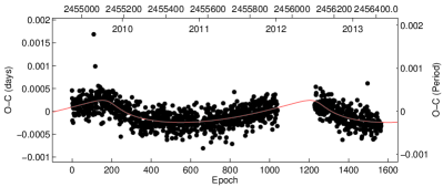
Figure 4.— The $O-C$ diagram of the Kepler minima times of the system KIC 5621294 after subtraction of the quadratic ephemerides.

The LC was fitted and analysed, resulted in the largest difference between the primary and secondary temperatures of the eclipsing components in our sample of stars. From the LC parameters written in Table 2 one can see a non-negligible value of the third light and only very weak contribution of the secondary component to the total light. On the other hand, the times of minima as derived from the Kepler data show a significant period decrease (described via parabolic ephemerides), see Fig. 3. Moreover, superposing over the parabola also a small periodic variation is visible with period of about 2.7 yr and the lowest amplitude in our sample (about 21 seconds only), see Fig. 4. This small amplitude yielded also a small value of the predicted third light value, hence a third light contribution as detected during the LC solution should probably be attributed to another body in the system or a close visual component. However, it is still rather premature to speculate that we deal here with a real quadruple system. Such a low amplitude of the variation in the $O-C$ diagram could also serve as a testing example of what can be even discovered from the Kepler data by these classical techniques with eclipsing binaries: assuming the component masses $M_{1}=M_{2}=1M_{\odot}$ then the minimum third-body mass (i.e. assuming $i=90^{\circ}$) resulted in $M_{3,min}=0.039~{}M_{\odot}$, hence a typical brown dwarf mass.

6.5. KIC 7630658

The system KIC 7630658 was discovered by Slawson et al. (2011) from the Kepler data. No other analysis was carried out and our knowledge about the system is very limited. It is the faintest star in our sample.

The shape of the LC as obtained by the Kepler satellite clearly shows two well-defined minima, hence also the derivation of the times of minima was rather straight-forward. The final parameters are given in Table 2, where one can see that both components are similar to each other and only a small fraction of the third light was detected. The variation with period of about 2.5 yr is clearly visible on the data, however our last observation slightly deviates from the prediction. This can be caused by some long-term modulation of the orbital period (quadratic ephemerides), but this have to be tested in the upcoming years with new observations.

6.6. KIC 8553788

The star KIC 8553788 was first mentioned as an eclipsing binary by Pigulski et al. (2009). Later, only the results from the Kepler data analysis were published: Slawson et al. (2011), Prša et al. (2011), and Gies et al. (2012). The latter paper gives some information about possible pulsations, starspots and possible third body. This system seems to be of the earliest spectral type in our sample of stars (see Table 1).

Our analysis using the Kepler data yielded the LC solution showing that the primary is the dominant object in the system, hence only the primary minima were used for the $O-C$ diagram analysis. The 9-yr variation is clearly visible in the plot despite the fact that the orbital period is still determined only by the one last observation from the Ondřejov Observatory. The older observations from the ASAS and SuperWASP surveys only slightly follow the predicted fit, but have quite large scatter. Our fit of minima times yielded rather high value of eccentricity, however the minimal third-body mass as resulted from the mass function is somewhat lower than the masses of the eclipsing components. Its light contribution hence should probably be higher than resulted from our LC fit.

6.7. KIC 9007918

The star KIC 9007918 (also TYC 3541-2296-1) was first detected as a variable by Devor et al. (2008) on the basis of the TRES survey data. Later, the star was included into the catalogue of Kepler eclipsing binaries (Slawson et al. 2011, and Prša et al. 2011).

There were detected some variations on the LC during the Kepler mission, and the whole LC is not perfectly symmetric. This can also play some role on the precision of the derived times of minima from the LC template. As one can also see from the LC, the secondary minimum is only very shallow, hence we used only the primary ones for analysing the period changes in this binary. Together with the old (and rather scattered) photometry from the TRES survey we were able to detect the periodic variations with the period of about 1.3 yr and an amplitude of about 41 seconds only. The other interesting issue is also the value of period for a possible dynamical interaction between the orbits $P_{3}^{2}/P\sim 445$ yr. Hence, we can hope to find some changes after several decades of observations.

6.8. KIC 9402652

The star KIC 9402652 (also V2281 Cyg) was discovered as a variable already in the pre-Kepler era and a few observations of the minima of this star were published. It was mentioned in the list of stars observed by the ROTSE survey (Diethelm, 2001), later Pigulski et al. (2009) included the star into their ASAS observations of the Kepler fields, and the times of minima were published by Gies et al. (2012) and Conroy et al. (2014).

As one can see, the system consists of two almost identical stars, both temperatures and luminosities are practically the same. From this reason, also both the minima are very similar, hence both primary and secondary were used for the period analysis. We also collected the older published minima together with the photometry from the NSVS, SuperWASP, and ASAS surveys. Thanks to the large data set of available times of minima observations this system seems to be the richest one in our sample of stars (and with the data coverage ranging over more than 15 years). The $O-C$ diagram together with our new observations clearly shows the 4-yr variation, but with rather high eccentricity.

6.9. KIC 10581918

The system KIC 10581918 (also WX Dra) was discovered as a variable as early as in 1960 by Tsesevich (1960). Since than a few observations of the minima were published, but no light curve nor spectroscopic analysis of the system. Due to very deep primary eclipse of this star (1.67 mag) also the older visual and photographic observations can be reliable for the analysis of the period changes. The very first preliminary results were published in the conference proceedings (Wolf et al. 2015).

As one can see from the results of our analysis, the period of the third body is of about 14 yr (the longest one in our sample) and is now well-covered, but its amplitude is only poorly defined with our data. New minima times observations in the upcoming years can help us to better derive the amplitude of variations. However, the predicted mass function of the third body resulted in rather low value, hence also a non-detection of the third light in the LC solution is something expectable.

6.10. KIC 10686876

The eclipsing binary KIC 10686876 was first mentioned by Devor et al. (2008), based on the TRES survey data. Later, the star was included into the Kepler eclipsing binary database, Prša et al. (2011), and Slawson et al. (2011). Gies et al. (2012) published the minima times for the system, but no other information or analysis was performed.

The star seems to be the only one system in our sample which shows total eclipse. Due to this reason also the error of the inclination from the LC fit is very small. On the other hand, the secondary component is probably a very small star and the primary is the dominating one. As one can also see, the primary eclipses are rather deep and provide us much better times of minima than the secondaries. Hence, analysing the available minima from the Kepler, TRES, SuperWASP, and our new data (two from Ondřejov, two from the BOOTES-1A and BOOTES-2 telescopes in Spain) we obtained a set of third-body parameters given in Table 3 and the final fit presented in Fig. 3. The variation with a period of about 6.7 yr is now clearly visible in the current data set and the shape of the $O-C$ variation should easily be confirmed and the parameters improved by a few new observations obtained during the upcoming years.

7. Discussion and conclusions

Ten selected binaries were found to be worth of study due to the presence of the distant components, which cause the periodic modulation of their eclipsing periods. The periods of the third bodies (from 1 to 14 years) are usually adequately covered with the Kepler and the ground-based data, so the variation is certain nowadays. However, its origin is still questionable in several cases. This especially applies to such systems where the predicted mass function of the third body and the non/detected third light from the LC solution contradict each other. However, this can be caused by some of these reasons: 1. the imperfect LC fit (for these binaries with slightly asymmetric LC), 2. not very well-defined third body variation in the $O-C$ diagram (especially in these cases where the variation is mostly determined by the older scattered ground-based data), 3. the variation in the $O-C$ diagram incorrectly described (i.e. missing quadratic term or a fourth-body variation), 4. exotic object as the distant body (or also a binary, hence having much lower luminosity), or 5. some other phenomena modulating the period variation in the $O-C$ diagram (such as magnetic or other activity of the components). As a by-product of our analysis, there were found a few more systems, where the $O-C$ variation was not found, or is still questionable yet. These are summarized in Table 4. Regrettably, this is still too limited sample to do any reliable statistical analysis of incompleteness of triple systems found in the Kepler data.

At this point it would be useful to mention that when using the ”Method 1” as introduced in Section 3, some of the systems also have the short cadence data in the Kepler photometric database. Using the short cadence produces much more precise minima derivation (these minima times are labelled as ”Kepler SC” in the Appendix table with minima), but can also reveal some other phenomena non-detectable in the long cadence data. This happened for KIC 8553788 and KIC 10686876, for which some short time variation was detected on the short cadence data (probably $\delta$ Sct pulsations), which were not visible on the long cadence one. However, such additional variation also influences the light curve fitting and its precision.

Table 4Some other analysed systems.

System	Other ID	Remark
KIC 04245897	V583 Lyr	some variation with period about 50 yr found, but based only on older photographic data
KIC 06187893	TYC 3128-1653-1	quadratic ephemerides or third body with long period, not very convincing, new data needed
KIC 06852488	2MASS J19135355+4222482	some variation detected, but period still uncertain, more data needed
KIC 07258889	2MASS J18510630+4248400	some variation found, but showing rather non-periodic modulation
KIC 07938468	V481 Lyr	quadratic ephemerides based also on older photographic data
KIC 08552540	V2277 Cyg	no variation found
KIC 09101279	V1580 Cyg	some variation found, but not very convincing, older data too scattered
KIC 09602595	V0995 Cyg	variation with period 13.3 yr found, but the data before 1970 are in contradiction
KIC 09899416	BR Cyg	no variation found
KIC 10736223	V2290 Cyg	quadratic ephemerides only, based on older visual data
KIC 11913071	V2365 Cyg	no variation found
KIC 12071006	V379 Cyg	some variation detected only on the Kepler data, older measurements too scattered

One has to consider also the limitations of the method used for the analysis. The LC fit is a crucial issue, because it is used to derive the minima times for a subsequent analysis. However, the LC fits can also be the problematic issue, because we are dealing with pure photometry with no information about the individual masses of the components. Hence, fixing the mass ratio value $q=1$ is in fact only the first rough simplification. Therefore, having no information about the individual masses, also the mass function of the third body provides only very preliminary information about such object. Due to this reason and because of the unknown distance also the angular separation of the third component cannot be computed for a prospective interferometric detection. However, it should probably be hard to detect such bodies due to relative faintness of most of the stars for this technique.

To conclude, only dedicated high-dispersion, and high-S/N spectroscopic observations and a subsequent analysis can tell us something more about these objects and reveal their true nature. Moreover, also some new photometric observations in the upcoming years would be of great benefit, especially in these systems where the period variation is still not very certain yet and also for the dynamically interesting systems like KIC 3440230.

Appendix A Tables of minima

Table 5List of the minima timings used for the analysis. A sample what is included in the online data repository.

Star	BJD -	Error	Type	Filter∗	Source /
	2400000	[day]			Observatory
KIC 2305372	52802.67112	0.08710	Prim	I	Hatnet
KIC 2305372	52806.88251	0.07516	Prim	I	Hatnet
KIC 2305372	52809.68474	0.02068	Prim	I	Hatnet
KIC 2305372	52813.90357	0.06025	Prim	I	Hatnet
KIC 2305372	52816.71288	0.02019	Prim	I	Hatnet
KIC 2305372	52820.92775	0.03789	Prim	I	Hatnet
KIC 2305372	52823.74173	0.04552	Prim	I	Hatnet
KIC 2305372	52827.95039	0.03124	Prim	I	Hatnet
KIC 2305372	52830.76181	0.10454	Prim	I	Hatnet
KIC 2305372	53986.89162	0.00559	Prim	I	ASAS
KIC 2305372	54349.28814	0.00479	Prim	I	ASAS
KIC 2305372	54232.70365	0.04672	Prim	W	SuperWASP
KIC 2305372	54249.55658	0.21725	Prim	W	SuperWASP
KIC 2305372	54256.58249	0.32321	Prim	W	SuperWASP
KIC 2305372	54280.46490	0.30372	Prim	W	SuperWASP
KIC 2305372	54284.67542	0.29591	Prim	W	SuperWASP
KIC 2305372	54287.48710	0.08857	Prim	W	SuperWASP
KIC 2305372	54964.55486	0.00138	Prim	K	Kepler
KIC 2305372	54965.95912	0.00058	Prim	K	Kepler
KIC 2305372	54967.36384	0.00094	Prim	K	Kepler
KIC 2305372	54968.76843	0.00066	Prim	K	Kepler
KIC 2305372	54970.17336	0.00101	Prim	K	Kepler
KIC 2305372	54971.57795	0.00067	Prim	K	Kepler
KIC 2305372	54972.98267	0.00062	Prim	K	Kepler
KIC 2305372	54974.38726	0.00070	Prim	K	Kepler
KIC 2305372	54975.79185	0.00079	Prim	K	Kepler
KIC 2305372	54977.19678	0.00085	Prim	K	Kepler
KIC 2305372	54978.60149	0.00091	Prim	K	Kepler
KIC 2305372	54980.00574	0.00073	Prim	K	Kepler
KIC 2305372	54981.41067	0.00086	Prim	K	Kepler
KIC 2305372	54982.81537	0.00039	Prim	K	Kepler
KIC 2305372	54984.21996	0.00110	Prim	K	Kepler
KIC 2305372	54985.62488	0.00070	Prim	K	Kepler
KIC 2305372	54987.02981	0.00062	Prim	K	Kepler
KIC 2305372	54988.43405	0.00086	Prim	K	Kepler
KIC 2305372	54989.83910	0.00070	Prim	K	Kepler
KIC 2305372	54991.24321	0.00047	Prim	K	Kepler
KIC 2305372	54992.64825	0.00082	Prim	K	Kepler
KIC 2305372	54994.05283	0.00069	Prim	K	Kepler
KIC 2305372	54995.45753	0.00078	Prim	K	Kepler
KIC 2305372	54996.86211	0.00067	Prim	K	Kepler
KIC 2305372	55003.88545	0.00040	Prim	K	Kepler
KIC 2305372	55005.29049	0.00020	Prim	K	Kepler
KIC 2305372	55006.69480	0.00014	Prim	K	Kepler
KIC 2305372	55008.09956	0.00012	Prim	K	Kepler
KIC 2305372	55009.50452	0.00014	Prim	K	Kepler
KIC 2305372	55010.90921	0.00032	Prim	K	Kepler
KIC 2305372	55012.31376	0.00023	Prim	K	Kepler
KIC 2305372	55013.71867	0.00016	Prim	K	Kepler
KIC 2305372	55017.93246	0.00021	Prim	K	Kepler
KIC 2305372	55019.33701	0.00035	Prim	K	Kepler
KIC 2305372	55020.74184	0.00027	Prim	K	Kepler
KIC 2305372	55022.14659	0.00014	Prim	K	Kepler
KIC 2305372	55023.55113	0.00026	Prim	K	Kepler
KIC 2305372	55024.95602	0.00013	Prim	K	Kepler
KIC 2305372	55026.36035	0.00046	Prim	K	Kepler
KIC 2305372	55027.76524	0.00028	Prim	K	Kepler
KIC 2305372	55029.16978	0.00028	Prim	K	Kepler
KIC 2305372	55030.57440	0.00024	Prim	K	Kepler
KIC 2305372	55031.97912	0.00021	Prim	K	Kepler
KIC 2305372	55033.38386	0.00022	Prim	K	Kepler
KIC 2305372	55034.78833	0.00034	Prim	K	Kepler
KIC 2305372	55036.19320	0.00030	Prim	K	Kepler
KIC 2305372	55037.59793	0.00027	Prim	K	Kepler
KIC 2305372	55039.00247	0.00034	Prim	K	Kepler
KIC 2305372	55040.40708	0.00019	Prim	K	Kepler
KIC 2305372	55041.81186	0.00021	Prim	K	Kepler
KIC 2305372	55043.21665	0.00019	Prim	K	Kepler
KIC 2305372	55044.62138	0.00011	Prim	K	Kepler
KIC 2305372	55046.02599	0.00028	Prim	K	Kepler
KIC 2305372	55047.43055	0.00016	Prim	K	Kepler
KIC 2305372	55048.83520	0.00029	Prim	K	Kepler
KIC 2305372	55050.23952	0.00043	Prim	K	Kepler
KIC 2305372	55051.64437	0.00034	Prim	K	Kepler
KIC 2305372	55053.04903	0.00012	Prim	K	Kepler
KIC 2305372	55054.45394	0.00020	Prim	K	Kepler
KIC 2305372	55055.85838	0.00008	Prim	K	Kepler
KIC 2305372	55057.26288	0.00050	Prim	K	Kepler
KIC 2305372	55058.66788	0.00016	Prim	K	Kepler
KIC 2305372	55060.07257	0.00038	Prim	K	Kepler
KIC 2305372	55061.47687	0.00042	Prim	K	Kepler

Note: * W and K stand for special filters used for SuperWASP and Kepler.

References

- Borovička et al. (1988) Borovička, J., et al. 1988, CoBrn, 28, 1
- Borucki et al. (2010) Borucki, W. J., Koch, D., Basri, G., et al. 2010, Science, 327, 977
- Brát et al. (2009) Brát, L., Trnka, J., Lehký, M., et al. 2009, OEJV, 107, 1
- Brown et al. (2011) Brown, T. M., Latham, D. W., Everett, M. E., & Esquerdo, G. A. 2011, AJ, 142, 112
- Conroy et al. (2014) Conroy, K. E., Prša, A., Stassun, K. G., et al. 2014, AJ, 147, 45
- Devor et al. (2008) Devor, J., Charbonneau, D., O’Donovan, F. T., Mandushev, G., & Torres, G. 2008, AJ, 135, 850
- Diethelm (1996) Diethelm, R. 1996, BBSAG, 113, 1
- Diethelm (2001) Diethelm, R. 2001, IBVS, 5060, 1
- Diethelm (2001) Diethelm, R. 2001, BBSAG, 125, 1
- Diethelm (2014) Diethelm, R. 2014, IBVS, 6093, 1
- Samus et al. (2012) Samus N.N., Durlevich O.V., Kazarovets E V., et al. General Catalog of Variable Stars (GCVS database, Version 2012Feb)
- Gies et al. (2012) Gies, D. R., Williams, S. J., Matson, R. A., et al. 2012, AJ, 143, 137
- Guinan & Engle (2006) Guinan, E. F., & Engle, S. G. 2006, Ap&SS, 304, 5
- Hartman et al. (2004) Hartman, J. D., Bakos, G., Stanek, K. Z., & Noyes, R. W. 2004, AJ, 128, 1761
- Hübscher et al. (2012) Hübscher, J., Lehmann, P. B., & Walter, F. 2012, IBVS, 6010, 1
- Hübscher & Lehmann (2012) Hübscher, J., & Lehmann, P. B. 2012, IBVS, 6026, 1
- Hübscher et al. (2013) Hübscher, J., Braune, W., & Lehmann, P. B. 2013, IBVS, 6048, 1
- Hübscher & Lehmann (2013) Hübscher, J., & Lehmann, P. B. 2013, IBVS, 6070, 1
- Irwin (1959) Irwin, J. B. 1959, AJ, 64, 149
- Kotková & Wolf (2006) Kotková, L., & Wolf, M. 2006, IBVS, 5676, 1
- Kwee & van Woerden (1956) Kwee, K. K., & van Woerden, H. 1956, BAN, 12, 327
- Liao & Qian (2010) Liao, W.-P., & Qian, S.-B. 2010, MNRAS, 405, 1930
- Locher (1990) Locher, K. 1990, BBSAG, 94, 1
- Locher (1992) Locher, K. 1992, BBSAG, 99, 1
- Locher (1995) Locher, K. 1995, BBSAG, 109, 1
- Locher (2005) Locher, K. 2005, OEJV, 3, 1
- Mayer (1990) Mayer, P. 1990, BAICz, 41, 231
- Mikulášek et al. (1992) Mikulášek, Z., Šilhán, J., Zejda, M. 1992, CoBrn, 30, 1
- Paschke & Brát (2006) Paschke, A., & Brát, L. 2006, OEJV, 23, 13
- Pickles & Depagne (2010) Pickles, A., & Depagne, É. 2010, PASP, 122, 1437
- Pigulski et al. (2009) Pigulski, A., Pojmański, G., Pilecki, B., & Szczygieł, D. M. 2009, AcA, 59, 33
- Pojmanski (2002) Pojmanski, G. 2002, AcA, 52, 397
- Pollacco et al. (2006) Pollacco, D. L., et al. 2006, PASP, 118, 1407
- Prša & Zwitter (2005) Prša, A., Zwitter, T. 2005, ApJ, 628, 42
- Prša et al. (2011) Prša, A., Batalha, N., Slawson, R. W., et al. 2011, AJ, 141, 83
- Rappaport et al. (2013) Rappaport, S., Deck, K., Levine, A., et al. 2013, ApJ, 768, 33
- Skrutskie et al. (2006) Skrutskie, M. F., Cutri, R. M., Stiening, R., et al. 2006, AJ, 131, 1163
- Slawson et al. (2011) Slawson, R. W., Prša, A., Welsh, W. F., et al. 2011, AJ, 142, 160
- Söderhjelm (1975) Söderhjelm, S. 1975, A&A, 42, 229
- Šafář & Zejda (2000) Šafář, J., & Zejda, M. 2000, IBVS, 4888, 1
- Terrell & Wilson (2005) Terrell, D., & Wilson, R. E. 2005, Ap&SS, 296, 221
- Tsesevich (1960) Tsesevich, V. P. 1960, Astronomicheskij Tsirkulyar, 210, 22
- van Hamme (1993) van Hamme, W. 1993, AJ, 106, 2096
- Wilson & Devinney (1971) Wilson, R. E., & Devinney, E. J. 1971, ApJ, 166, 605
- Wolf et al. (2015) Wolf, M., Zasche, P., Vraštil, J., Kučáková, H., & Hornoch, K. 2015, ASP conference series, in press
- Woźniak et al. (2004) Woźniak, P. R., Vestrand, W. T., Akerlof, C. W., et al. 2004, AJ, 127, 2436
- Zasche et al. (2011) Zasche, P., Uhlář, R., Kučáková, H., & Svoboda, P. 2011, IBVS, 6007, 1
- Zasche et al. (2014) Zasche, P., Wolf, M., Vraštil, J., et al. 2014, A&A, 572, A71