Relativistic Causal Hydrodynamics Derived from Boltzmann Equation: a novel reduction theoretical approach

Abstract

We derive the second-order hydrodynamic equation and the microscopic formulae of the relaxation times as well as the transport coefficients systematically from the relativistic Boltzmann equation. Our derivation is based on a novel development of the renormalization-group method, a powerful reduction theory of dynamical systems, which has been applied successfully to derive the non-relativistic second-order hydrodynamic equation. Our theory nicely gives a compact expression of the deviation of the distribution function in terms of the linearized collision operator, which is different from those used as an ansatz in the conventional fourteen-moment method. It is confirmed that the resultant microscopic expressions of the transport coefficients coincide with those derived in the Chapman-Enskog expansion method. Furthermore, we show that the microscopic expressions of the relaxation times have natural and physically plausible forms. We prove that the propagating velocities of the fluctuations of the hydrodynamical variables do not exceed the light velocity, and hence our second-order equation ensures the desired causality. It is also confirmed that the equilibrium state is stable for any perturbation described by our equation.

I Introduction

The experiments of relativistic heavy ion collision at the Relativistic Heavy Ion Collider (RHIC) at Brookhaven National Laboratory and the Large Hadron Collider (LHC) at CERN seem to have created a hot matter that is most likely to be composed of quarks and gluons, i.e., the quark-gluon plasma (QGP) Shuryak (2004); Gyulassy and McLerran (2005). One of the most surprising findings is that the created matter is well described by the hydrodynamics with tiny dissipation Bass and Dumitru (2000); Teaney et al. (2001); Teaney (2003); Hirano and Gyulassy (2006); Hirano et al. (2006); Nonaka and Bass (2007); Baier et al. (2006, 2007); Baier and Romatschke (2007); Romatschke (2007); Romatschke and Romatschke (2007); Bozek (2012); Hirano et al. (2013). Such a finding prompted an interest in the origin of the viscosity in the gauge theories and also the dissipative hydrodynamic equation. The relativistic dissipative hydrodynamic equation is also utilized in analyzing various high-energy astrophysical phenomena Balsara (2001) including the accelerated expansion of the universe by bulk viscosity of dark matter and/or dark energy Fabris et al. (2006); Colistete et al. (2007).

One must say, however, that the theory of relativistic hydrodynamics for a viscous fluid has not been established on a firm ground yet, although there have been many important studies since Eckart’s pioneering work Eckart (1940): A naive relativistic extension of the Navier-Stokes equation has fundamental problems such as ambiguity of flow velocity Eckart (1940); Landau (1959); Van and Biro (2012); Osada (2012), existence of unphysical instabilities Hiscock and Lindblom (1985), and lack of causality Israel (1976); Israel and Stewart (1979), the last of which motivated people to introduce the second-order hydrodynamic equation. The way of formulation of the second-order hydrodynamics is, however, controversial and an established equation has not been obtained although some suggestive and promising approaches have been proposed.

It is worth emphasizing here that the second-order hydrodynamic equation that is free from the causality problem even in the non-relativistic regime is not yet established, either. The causality problem inherent in the first-order equation, which we call generically the Navier-Stokes equation, appears as the instantaneous propagation of information, which is attributed to parabolicity of the equation Stewart (1971); Cattaneo (1958); Muller (1967); Müller and Ruggeri (1993). In the seminal paper by Grad Grad (1949), he showed that the causality problem could be circumvented by the moment method, which now bears his name: It is found that the thirteen-moment approximation to the functional forms of the distribution function leads to a hyperbolic non-relativistic equation satisfying the causality, with finite propagation speeds of physical quantities. Here, we make a sideremark that the description by the Grad equation may be called mesoscopic Jou et al. (1996); Dedeurwaerdere et al. (1996) since it occupies an intermediate level between the descriptions by the Navier-Stokes equation and the Boltzmann equation; see also Balescu (1988). It should be noted, however, that the dynamics described by the Grad equation has been recently shown inconsistent with the underlying Boltzmann equation in the mesoscopic scales of space and time Torrilhon (2009). Indeed, Grad’s moment method lacks a principle for determining the functional form of the distribution function that is consistent with the underlying Boltzmann equation, and then it is inevitable for the moment method to adopt an ad-hoc but seemingly plausible ansatz for it. Although there are subsequent attempts to construct the equation that respects both of the causality and the consistency with the Boltzmann equation in the mesoscopic regime Struchtrup and Torrilhon (2003); Levermore (1996); Torrilhon (2010); Öttinger (2010), the consistency between the resultant equations and the mesoscopic dynamics of the Boltzmann equation remains unclear.

Nevertheless, many attempts were made to extend Grad’s moment method to establish a mesoscopic description of a relativistic system Israel (1976); Israel and Stewart (1979); Huovinen and Molnar (2009); Molnar and Huovinen (2009); El et al. (2010); Bouras et al. (2010); Denicol et al. (2012a); Denicol et al. (2010); Denicol et al. (2012b); Pu et al. (2010), but with only a partial success, as anticipated. For instance, the celebrated Israel-Stewart equation Israel and Stewart (1979), which is a typical second-order relativistic hydrodynamic equation derived from the Boltzmann equation based on the moment method with fourteen moments employed is found to be incomplete if not incorrect because the solutions behave differently from those of the relativistic Boltzmann equation quantitatively Huovinen and Molnar (2009); Molnar and Huovinen (2009); El et al. (2010). The incompleteness or incorrectness can be traced back to ambiguous heuristic assumptions inherent in the moment method. Quite recently, however, some heuristic but promising methods have been proposed Denicol et al. (2010); Denicol et al. (2012b); Jaiswal (2013) to get rid of such drawbacks, and it seems that the resultant solutions indeed become closer to that of the Boltzmann equation. Although their results are encouraging, one must say that their derivation are still based on plausible but ambiguous assumptions that require a microscopic foundation. In fact, the constitutive equations contain the second-order spatial derivatives of the hydrodynamical variables, which necessarily leads to the parabolicity that should have been avoided.

Recently, the mesoscopic dynamics or the second-order dynamics that respects the causality has been extracted from the Boltzmann equation for the non-relativistic case in the classical regime without recourse to any ansatz for the functional forms of the distribution function by two of the present authors Tsumura and Kunihiro (2013a): There “the renormalization-group (RG) method” Chen et al. (1994, 1996); Kunihiro (1995, 1997); Kunihiro and Matsukidaira (1998); Kunihiro (1998a, b); Boyanovsky et al. (1999); Goto et al. (1999); Ei et al. (2000); Boyanovsky et al. (2000); Ziane (2000); Nozaki and Oono (2001); Hatta and Kunihiro (2002); Boyanovsky and de Vega (2003); Kunihiro and Tsumura (2006); DeVille et al. (2008); Chiba (2008, 2009) was adopted as a powerful method of the reduction theory of dynamical systems to reduce the Boltzmann equation to the mesoscopic dynamics. The basic observation in these works is that the first-order hydrodynamics is the slow dynamics achieved asymptotically in the kinetic equation Hatta and Kunihiro (2002); Kunihiro and Tsumura (2006): The asymptotic dynamics is described by the zero modes of the linearized collision operator, which happen to be temperature, density, and fluid velocity, i.e., the hydrodynamic variables. In terms of the reduction theory of dynamical systems Kuramoto (1989), it means that the hydrodynamic variables constitute the natural coordinates of the invariant/attractive manifold of the space of the distribution function in which the asymptotic dynamics in the hydrodynamical regime is described. In the RG method, the hydrodynamic variables, which is now the would-be zero modes, acquire the time dependence by the RG equation. The resultant evolution equation is nothing but the hydrodynamic equation, the Navier-Stokes equation. Then, the extension to the extraction of the mesoscopic dynamics consists of developing the way to include some excited (fast) modes properly as additional components of the invariant/attractive manifold; note that the mesoscopic dynamics is faster than that described by the Navier-Stokes equation. In Tsumura and Kunihiro (2013a), the following natural conditions are found to give the adequate excited modes to be incorporated in the hydrodynamical variables in the classical and non-relativistic case: (A) the resultant dynamics should be consistent with the reduced dynamics obtained by employing only the zero modes in the asymptotic regime; (B) the resultant dynamics should be as simple as possible because we are interested to reduce the dynamics to a simpler one; the term “simple” means that the resultant dynamics is described with a fewer number of dynamical variables and is given by an equation composed of a fewer number of terms. Here, we note that the latter principle (B) is one of the fundamental principle of the reduction theory of the dynamics as emphasized by Kuramoto Kuramoto (1989). It was shown that these conditions lead to a concise scheme called the doublet scheme, and that the resultant equation with thirteen dynamical variables satisfies the causality in an apparent way and has the same form as that of the Grad equation but with different microscopic formulae of the transport coefficients and relaxation times; the expressions of the transport coefficients coincide with those by the Chapman-Enskog method Chapman and Cowling (1970), the novel formulae of the relaxation times allow a natural physical interpretation as the relaxation times. This is an encouraging result!

A comment is in order here on the relation between this work and Tsumura and Kunihiro (2010) in which the two of the present authors (K.T. and T.K.) derived a second-order hydrodynamic equation from the relativistic Boltzmann equation on the basis of the RG method. The derivation presented in Tsumura and Kunihiro (2010), however, contained an inconclusive part which is, in retrospect, incorrect, unfortunately. Indeed the functional form of the excited modes was not determined so as to solve the Boltzmann equation but that adopted in the Israel-Stewart fourteen-moment method was mistakenly used as a possible solution: It is known that the Israel-Stewart ansatz does not solve the relativistic Boltzmann equation. In this work, we first find a proper solution to the relativistic Boltzmann equation in the relevant kinetic regime on the basis of an elaborated doublet scheme in the RG method, and thus derive the functional form of the excited modes that is consistent with the underlying Boltzmann equation. Then simply applying the RG equation, we obtain the second-order relativistic hydrodynamic equation, which accordingly gives the correct asymptotic dynamics of the Boltzmann equation in the mesoscopic regime.

The present paper is an extension of the previous work Tsumura and Kunihiro (2013a) to a relativistic case with the full quantum statistics as well as classical one. We here remark that preliminary results in the classical case were announced in Tsumura and Kunihiro (2012). Needless to say, the quantum statistics is essential in investigating the behavior of a quantum fluid composed of bosons and/or fermions. In the present paper, we shall give a detailed and complete account of the derivations of the causal hydrodynamic equations within the quantum and classical statistics together with those of the microscopic expressions of the transport coefficients and relaxation times. We shall also show that a concise and natural derivation is possible for the excited modes that is given by the doublet scheme Tsumura and Kunihiro (2013a) on the basis of the very principle of the reduction theory of the dynamics.

Moreover, we prove that the propagating velocities of the fluctuations of the hydrodynamical variables do not exceed the light velocity, and hence our seconder-order equation ensures the causality as desired. It is also shown that the equilibrium state is stable for any perturbation described by our equation. We give a compact expression of the deviation of the distribution function to be used in the fourteen-moment method.

This paper is organized as follows: In Sec. II, we briefly summarize the basics of the relativistic Boltzmann equation. In Sec. III, we derive the causal hydrodynamic equation by applying the doublet scheme in the RG method, and give the microscopic representations of the transport coefficients and relaxation times. Then the basic properties of the resultant equation including the causality are shown together with a comparison of the microscopic expressions with those given by other methods. We devote Sec. IV to a summary and concluding remarks. In Appendix A, we derive the functional forms of the excited modes which are given by the faithful solution of the Boltzmann equation. In Appendix B, the explicit solution is given for a linear equation with a time-dependent inhomogeneous term appearing in the text. In Appendix C, we present a detailed and lengthy derivation of the relaxation equations, which shows how the microscopic expressions of the relaxation times and lengths are obtained. In Appendix D, we give a proof that our second-order equation is really causal and that the static solution is stable against any fluctuations.

In this paper, we use the natural unit, i.e., $\hbar=c=k_{\mathrm{B}}=1$, and the Minkowski metric $g^{\mu\nu}=\mathrm{diag}(+1,-1,-1,-1)$.

II Preliminary

In this section, we summarize the basic facts about the relativistic Boltzmann equation de Groot et al. (1980).

II.1 Basics of relativistic Boltzmann equation

The relativistic Boltzmann equation reads de Groot et al. (1980); Cercignani and Kremer (2002)

$$p^{\mu}\partial_{\mu}f_{p}(x)=C[f]_{p}(x),$$ (1)

where $f_{p}(x)$ denotes the one-particle distribution function with $p^{\mu}$ being the four-momentum of the on-shell particle, i.e., $p^{\mu}p_{\mu}=p^{2}=m^{2}$ and $p^{0}>0$. The right-hand-side term $C[f]_{p}(x)$ denotes the collision integral

$$C[f]_{p}(x) \equiv\frac{1}{2!}\int\mathrm{d}p_{1}\mathrm{d}p_{2}\mathrm{d}p_{3}\omega(p,p_{1}|p_{2},p_{3})$$

$$\times((1+af_{p}(x))(1+af_{p_{1}}(x))f_{p_{2}}(x)f_{p_{3}}(x)$$

$$-f_{p}(x)f_{p_{1}}(x)(1+af_{p_{2}}(x))(1+af_{p_{3}}(x))),$$ (2)

where $\omega(p,p_{1}|p_{2},p_{3})$ is the transition probability due to the microscopic two-particle interaction with the symmetry property

$$\omega(p,p_{1}|p_{2},p_{3})=\omega(p_{2},p_{3}|p,p_{1})$$

$$=\omega(p_{1},p|p_{3},p_{2})=\omega(p_{3},p_{2}|p_{1},p),$$ (3)

and the energy-momentum conservation

$$\omega(p,p_{1}|p_{2},p_{3})\propto\delta^{4}(p+p_{1}-p_{2}-p_{3}),$$ (4)

and $a$ represents the quantum statistical effect, i.e., $a=+1$ for boson, $a=-1$ for fermion, and $a=0$ for the Boltzmann gas. In the following, we suppress the arguments $x$, and abbreviate an integration measure as

$$\mathrm{d}p\equiv\mathrm{d}^{3}\boldsymbol{p}/[(2\pi)^{3}p^{0}],$$ (5)

with $\boldsymbol{p}$ being the spatial components of the four momentum $p^{\mu}$ when no misunderstanding is expected.

For an arbitrary vector $\varphi_{p}$ foo , the collision integral satisfies the following identity thanks to the above-mentioned symmetry properties,

$$\int\mathrm{d}p\varphi_{p}C[f]_{p} =\frac{1}{2!}\frac{1}{4}\int\mathrm{d}p\mathrm{d}p_{1}\mathrm{d}p_{2}\mathrm{d}p_{3}\,\omega(p\,,\,p_{1}|p_{2}\,,\,p_{3})$$

$$\times(\varphi_{p}+\varphi_{p_{1}}-\varphi_{p_{2}}-\varphi_{p_{3}})$$

$$\times((1+af_{p})(1+af_{p_{1}})f_{p_{2}}f_{p_{3}}$$

$$-f_{p}f_{p_{1}}(1+af_{p_{2}})(1+af_{p_{3}})).$$ (6)

Substituting $(1,p^{\mu})$ into $\varphi_{p}$ in Eq. (II.1), we find that $(1,p^{\mu})$ are collision invariants satisfying

$$\int\mathrm{d}p\frac{1}{p^{0}}C[f]_{p} =0,$$ (7)

$$\int\mathrm{d}p\frac{1}{p^{0}}p^{\mu}C[f]_{p} =0,$$ (8)

due to the particle-number and energy-momentum conservation in the collision process, respectively. We note that the function $\varphi_{0p}\equiv\alpha(x)+p^{\mu}\beta_{\mu}(x)$ is also a collision invariant where $\alpha(x)$ and $\beta^{\mu}(x)$ are arbitrary functions of $x$.

Owing to the particle-number and energy-momentum conservation in the collision process leading to Eqs. (7) and (8), we have the balance equations

$$\partial_{\mu}N^{\mu} =0,$$ (9)

$$\partial_{\nu}T^{\mu\nu} =0,$$ (10)

where the particle current $N^{\mu}$ and the energy-momentum tensor $T^{\mu\nu}$ are defined by

$$N^{\mu} \equiv\int\mathrm{d}p\,p^{\mu}f_{p},$$ (11)

$$T^{\mu\nu} \equiv\int\mathrm{d}p\,p^{\mu}p^{\nu}f_{p},$$ (12)

respectively. It should be noted that any dynamical properties are not contained in these equations unless the evolution of $f_{p}$ has been obtained as a solution to Eq. (1).

In the Boltzmann theory, the entropy current may be defined de Groot et al. (1980) by

$$S^{\mu}\equiv-\int\mathrm{d}p\,p^{\mu}\Bigg{[}f_{p}\ln f_{p}-\frac{(1+af_{p})\ln(1+af_{p})}{a}\Bigg{]}.$$ (13)

The entropy current $S^{\mu}$ satisfies the divergence equation

$$\partial_{\mu}S^{\mu}=-\int\mathrm{d}p\,C[f]_{p}\ln\Bigg{[}\frac{f_{p}}{1+af_{p}}\Bigg{]},$$ (14)

because of Eq. (1). One sees that $S^{\mu}$ is conserved only if $\ln(f_{p}/(1+af_{p}))$ is a collision invariant, i.e., $\ln(f_{p}/(1+af_{p}))=\varphi_{0p}=\alpha(x)+p^{\mu}\beta_{\mu}(x)$. One thus finds de Groot et al. (1980); Cercignani and Kremer (2002) that the entropy-conserving distribution function can be parametrized as

$$f_{p}=\frac{1}{\mathrm{e}^{(p^{\mu}u_{\mu}-\mu)/T}-a}\equiv f^{\mathrm{eq}}_{p},$$ (15)

where $T$, $\mu$, and $u^{\mu}$ may depend on the space and time, and are interpreted as the local temperature, chemical potential, and flow velocity, respectively, with the normalization

$$u^{\mu}u_{\mu}=1.$$ (16)

Thus the function (15) is identified with the local equilibrium distribution function. We see that the collision integral identically vanishes for the local equilibrium distribution $f^{\mathrm{eq}}_{p}$ as

$$C[f^{\mathrm{eq}}]_{p}=0,$$ (17)

owning to the detailed balance

$$\omega(p,p_{1}|p_{2},p_{3})\big{[}(1+af^{\mathrm{eq}}_{p})(1+af^{\mathrm{eq}}_{p_{1}})f^{\mathrm{eq}}_{p_{2}}f^{\mathrm{eq}}_{p_{3}}$$

$$-f^{\mathrm{eq}}_{p}f^{\mathrm{eq}}_{p_{1}}(1+af^{\mathrm{eq}}_{p_{2}})(1+af^{\mathrm{eq}}_{p_{3}})\big{]}=0,$$ (18)

guaranteed by the energy-momentum conservation (4).

Substituting $f_{p}=f^{\mathrm{eq}}_{p}$ into Eqs. (11) and (12), we have

$$N^{\mu} =n\,u^{\mu}\equiv N^{\mu}_{0},$$ (19)

$$T^{\mu\nu} =eu^{\mu}u^{\nu}-P\Delta^{\mu\nu}\equiv T^{\mu\nu}_{0},$$ (20)

with

$$\Delta^{\mu\nu}\equiv g^{\mu\nu}-u^{\mu}u^{\nu}.$$ (21)

Here, $n$, $e$, and $P$ denote the particle-number density, internal energy, and pressure, respectively, whose microscopic representations are given by

$$n \equiv\int\mathrm{d}pf^{\mathrm{eq}}_{p}(p\cdot u)$$

$$=(2\pi)^{-3}4\pi m^{3}\sum_{k=1}^{\infty}a^{k-1}\mathrm{e}^{k\mu/T}(km/T)^{-1}K_{2}(km/T),$$ (22)

$$e \equiv\int\mathrm{d}pf^{\mathrm{eq}}_{p}(p\cdot u)^{2}$$

$$=mn\Bigg{[}\frac{\sum_{k=1}^{\infty}a^{k-1}\mathrm{e}^{k\mu/T}(km/T)^{-1}K_{3}(km/T)}{\sum_{l=1}^{\infty}a^{l-1}\mathrm{e}^{l\mu/T}(lm/T)^{-1}K_{2}(lm/T)}$$

$$-\frac{\sum_{k=1}^{\infty}a^{k-1}\mathrm{e}^{k\mu/T}(km/T)^{-2}K_{2}(km/T)}{\sum_{l=1}^{\infty}a^{l-1}\mathrm{e}^{l\mu/T}(lm/T)^{-1}K_{2}(lm/T)}\Bigg{]},$$ (23)

$$P \equiv\int\mathrm{d}pf^{\mathrm{eq}}_{p}(-p^{\mu}p^{\nu}\Delta_{\mu\nu}/3)$$

$$=mn\frac{\sum_{k=1}^{\infty}a^{k-1}\mathrm{e}^{k\mu/T}(km/T)^{-2}K_{2}(km/T)}{\sum_{l=1}^{\infty}a^{l-1}\mathrm{e}^{l\mu/T}(lm/T)^{-1}K_{2}(lm/T)},$$ (24)

with $K_{2}(z)$ and $K_{3}(z)$ being the second- and third-order modified Bessel functions. Setting $a=0$ in the above expressions, we can check that the classical expressions for $n$, $e$, and $P$ de Groot et al. (1980) are reproduced. We note that $N^{\mu}_{0}$ and $T^{\mu\nu}_{0}$ in Eqs. (19) and (20) are identical to those in the relativistic Euler equation, which describes the fluid dynamics without dissipative effects, and $n$, $e$, and $P$ defined by Eqs. (II.1)-(II.1) are the equations of state of the dilute gas. Since the entropy-conserving distribution function $f^{\mathrm{eq}}_{p}$ reproduces the relativistic Euler equation, we find that the dissipative effects are attributable to the deviation of $f_{p}$ from $f^{\mathrm{eq}}_{p}$.

III Relativistic causal hydrodynamics by doublet scheme in RG method

In this section, we derive the causal relativistic hydrodynamic equation as the mesoscopic dynamics from the relativistic Boltzmann equation (III.1.1): The derivation is based on the doublet scheme in the RG method developed for the non-relativistic case in Tsumura and Kunihiro (2013a); the present formulation is an extension to the relativistic case and given in a simplified and more transparent manner. We examine some properties of the resultant equation, concerning the frame, the stability of the equilibrium state, and the causality as well as the microscopic representations of the transport coefficients and the relaxation times. It will be noted that our formalism solving the Boltzmann equation gives the compact expression of the perturbed distribution function, which may be used in the moment method as the proper ansatz of the distribution function that can lead to the hydrodynamic equation consistent with the Boltzmann equation.

III.1 Reduced dynamics by RG method

III.1.1 Macroscopic-frame vector

Since we are interested in the hydrodynamic regime to be realized asymptotically where the time and space dependence of the physical quantities are small, we try to solve Eq. (1) in the situation where the space-time variation of $f_{p}(x)$ is small and the space-time scales are coarse-grained from those in the kinetic regime. To make a coarse graining with the Lorentz covariance being retained, we introduce a time-like Lorentz vector denoted by $\boldsymbol{a}^{\mu}$ with $\boldsymbol{a}^{2}>0$ and $\boldsymbol{a}^{0}>0$ Tsumura et al. (2007); Tsumura and Kunihiro (2011), which may depend on $x^{\mu}$; $\boldsymbol{a}^{\mu}=\boldsymbol{a}^{\mu}(x)$. Thus, $\boldsymbol{a}^{\mu}$ specifies the covariant but macroscopic coordinate system where the local rest frame of the flow velocity and/or the flow velocity itself are defined: Since such a coordinate system is called frame, we call $\boldsymbol{a}^{\mu}$ the macroscopic frame vector. In fact, with the use of $\boldsymbol{a}^{\mu}$, we define the covariant and macroscopic coordinate system $(\tau,\sigma^{\mu})$ from the space-time coordinate $x^{\mu}$ as $\mathrm{d}\tau\equiv\boldsymbol{a}^{\mu}\mathrm{d}x_{\mu}$ and $\mathrm{d}\sigma^{\mu}\equiv(g^{\mu\nu}-\boldsymbol{a}^{\mu}\boldsymbol{a}^{\nu}/\boldsymbol{a}^{2})\mathrm{d}x_{\nu}$, which lead to derivatives given by $\partial/\partial\tau=(\boldsymbol{a}^{\mu}/\boldsymbol{a}^{2})\partial_{\mu}$ and $\partial/\partial\sigma_{\mu}=(g^{\mu\nu}-\boldsymbol{a}^{\mu}\boldsymbol{a}^{\nu}/\boldsymbol{a}^{2})\partial_{\nu}$.

Then, the relativistic Boltzmann equation (1) in the new coordinate system $(\tau,\sigma^{\mu})$ is written as

$$p\cdot\boldsymbol{a}(\tau,\sigma)\frac{\partial}{\partial\tau}f_{p}(\tau,\sigma)+p^{\mu}\frac{\partial}{\partial\sigma^{\mu}}f_{p}(\tau,\sigma)=C[f]_{p}(\tau,\sigma),$$ (25)

where $\boldsymbol{a}^{\mu}(\tau,\sigma)\equiv\boldsymbol{a}^{\mu}(x)$ and $f_{p}(\tau,\sigma)\equiv f_{p}(x)$. We remark the prefactor of the time derivative is a Lorentz scalar and positive definite; $p\cdot\boldsymbol{a}(\tau,\sigma)>0$, which is easily verified by taking the rest frame of $p^{0}$.

Since we are interested in a hydrodynamic solution to Eq. (25) as mentioned above, we suppose that the time variation of $\boldsymbol{a}^{\mu}(\tau,\sigma)$ is much smaller than that of the microscopic processes and hence $\boldsymbol{a}^{\mu}(\tau,\sigma)$ has no $\tau$ dependence, i.e.,

$$\boldsymbol{a}^{\mu}(\tau,\sigma)=\boldsymbol{a}^{\mu}(\sigma).$$ (26)

Then, with the use of Eq. (26), we shall convert Eq. (25) into

$$\frac{\partial}{\partial\tau}f_{p}(\tau,\sigma) =\frac{1}{p\cdot\boldsymbol{a}(\sigma)}C[f]_{p}(\tau,\sigma)$$

$$-\epsilon\frac{1}{p\cdot\boldsymbol{a}(\sigma)}p^{\mu}\frac{\partial}{\partial\sigma^{\mu}}f_{p}(\tau,\sigma).$$ (27)

Here, the parameter $\epsilon$ is introduced for characterizing the smallness of the inhomogeneity of the distribution function, which may be identified with the ratio of the mean free path over the characteristic macroscopic length, i.e., the Knudsen number. Since $\epsilon$ appears in front of the second term of the right-hand side of Eq. (III.1.1), the relativistic Boltzmann equation has a form to which the perturbative expansion is applicable.

In the present analysis based on the RG method, the perturbative expansion of the distribution function with respect to $\epsilon$ is first performed with the zeroth-order solution being the local equilibrium one, which has no dissipative effects. The dissipative effects are taken into account in the higher orders; the spatial inhomogeneity as the perturbation gives rise to a deformation of the distribution function which is responsible for the dissipative effects. Note that the deformation also can trigger a relaxation toward the local equilibrium state. Thus, the above rewrite of the equation with $\epsilon$ reflects the physical assumption that only the spatial inhomogeneity plays dual roles as the origin of the dissipation and the cause of a relaxation to the local equilibrium state. It is noteworthy that our RG method applied to the non-relativistic Boltzmann equation with the corresponding assumption successfully leads to the non-relativistic causal hydrodynamic equation Tsumura and Kunihiro (2013a), which means that the present approach is simply a relativistic generalization of the non-relativistic case.

III.1.2 Construction of approximate solution around arbitrary initial time

In accordance with the general formulation of the RG method Kunihiro (1995, 1998a); Ei et al. (2000), let $f_{p}(\tau,\sigma)$ be an exact solution yet to be obtained with an initial condition set up, say at $\tau=-\infty$. Then we pick up an arbitrary time $\tau=\tau_{0}$ in the (asymptotic) hydrodynamic regime, and try to obtain the perturbative solution $\tilde{f}_{p}$ to Eq. (III.1.1) around the time $\tau=\tau_{0}$ with the initial condition

$$\tilde{f}_{p}(\tau=\tau_{0},\sigma;\tau_{0})=f_{p}(\tau_{0},\sigma),$$ (28)

where we have made explicit that the solution has the $\tau_{0}$ dependence. The initial value or the exact solution as well as the perturbative solution are expanded with respect to $\epsilon$ as follows;

$$\tilde{f}_{p}(\tau,\sigma;\tau_{0}) =\tilde{f}_{p}^{(0)}(\tau,\sigma;\tau_{0})+\epsilon\tilde{f}_{p}^{(1)}(\tau,\sigma;\tau_{0})$$

$$+\epsilon^{2}\tilde{f}_{p}^{(2)}(\tau,\sigma;\tau_{0})+\cdots,$$ (29)

$$f_{p}(\tau_{0},\sigma) =f_{p}^{(0)}(\tau_{0},\sigma)+\epsilon f_{p}^{(1)}(\tau_{0},\sigma)$$

$$+\epsilon^{2}f_{p}^{(2)}(\tau_{0},\sigma)+\cdots.$$ (30)

The respective initial conditions at $\tau=\tau_{0}$ are set up as

$$\tilde{f}_{p}^{(l)}(\tau_{0},\sigma;\tau_{0})=f_{p}^{(l)}(\tau_{0},\sigma),\,\,\,\,\,\,l=0,1,2,\cdots.$$ (31)

In the expansion, the zeroth-order value $\tilde{f}_{p}^{(0)}(\tau_{0},\sigma;\tau_{0})=f_{p}^{(0)}(\tau_{0},\sigma)$ is supposed to be as close as possible to an exact solution $f_{p}(\tau,\sigma)$. In the RG method, the globally valid solution is constructed by patching the local solutions $\tilde{f}_{p}^{(0)}(\tau,\sigma;\tau_{0})$ which are only valid around $\tau=\tau_{0}$, which is tantamount to making an envelope curve of the perturbative solutions with $\tau_{0}$ being the parameter characterizing the perturbative trajectories Kunihiro (1995, 1998a).

Substituting the above expansions into Eq. (III.1.1) we obtain the series of the perturbative equations with respect to $\epsilon$, where the macroscopic frame vector is now replaced by a $\tau$-independent but $\tau_{0}$-dependent one Tsumura et al. (2007); Tsumura and Kunihiro (2011)

$$\boldsymbol{a}^{\mu}(\sigma)=\boldsymbol{a}^{\mu}(\sigma;\tau_{0}).$$ (32)

We have now a hierarchy of equations in order by order of $\epsilon$. As is mentioned before, our strategy to obtain the mesoscopic dynamics is constructing it as a minimal extension of the hydrodynamic one that is to be realized asymptotically after a long time within the Boltzmann equation. Notice that the hydrodynamics is a closed slow dynamics described solely by the would-be zero modes of the linearized collision operator corresponding to the conservation laws. The slowest dynamics will be given as a stationary solution, which actually exists for the zeroth order equation; the stationary solution is nothing but the local equilibrium one Tsumura et al. (2007); Tsumura and Kunihiro (2011). In our way of the solution of the Boltzmann equation on the perturbation theory with the single expansion parameter $\epsilon$, the deviation of the distribution function from the local equilibrium one is caused by the spatial inhomogeneity as given by the perturbative term in Eq. (III.1.1) and hence is proportional to $\epsilon$. We shall show that this setting of the analysis successfully solves the Boltzmann equation in a consistent way and leads to the mesoscopic dynamics.

With the above order counting in mind, let us construct the perturbative solution in the asymptotic regime order by order. The zeroth-order equation reads

$$\frac{\partial}{\partial\tau}\tilde{f}^{(0)}_{p}(\tau,\sigma;\tau_{0})=\frac{1}{p\cdot\boldsymbol{a}(\sigma;\tau_{0})}C[\tilde{f}^{(0)}]_{p}(\tau,\sigma;\tau_{0}).$$ (33)

Since we are interested in the slow motion which would be realized asymptotically as $\tau\rightarrow\infty$, we should take the following stationary solution,

$$\frac{\partial}{\partial\tau}\tilde{f}_{p}^{(0)}(\tau,\sigma;\tau_{0})=0,$$ (34)

which is realized when $\tilde{f}_{p}^{(0)}(\tau,\sigma;\tau_{0})$ is the fixed point,

$$\frac{1}{p\cdot\boldsymbol{a}(\sigma;\tau_{0})}C[\tilde{f}^{(0)}]_{p}(\tau,\sigma;\tau_{0})=0,$$ (35)

for arbitrary $\sigma$. We see that Eq. (35) is identical to Eq. (17), and hence $\tilde{f}_{p}^{(0)}(\tau,\sigma;\tau_{0})$ is found to be the local equilibrium distribution function (15):

$$\tilde{f}_{p}^{(0)}(\tau,\sigma;\tau_{0}) =f^{\mathrm{eq}}_{p}(\sigma;\tau_{0})$$

$$=\frac{1}{\mathrm{e}^{[p^{\mu}u_{\mu}(\sigma;\tau_{0})-\mu(\sigma;\tau_{0})]/T(\sigma;\tau_{0})}-a},$$ (36)

with $u^{\mu}(\sigma;\tau_{0})u_{\mu}(\sigma;\tau_{0})=1$, which implies that

$$f_{p}^{(0)}(\tau_{0},\sigma)=\tilde{f}_{p}^{(0)}(\tau=\tau_{0},\sigma;\tau_{0})=f^{\mathrm{eq}}_{p}(\sigma;\tau_{0}).$$ (37)

The five would-be integral constants $T(\sigma;\tau_{0})$, $\mu(\sigma;\tau_{0})$, and $u_{\mu}(\sigma;\tau_{0})$ are independent of $\tau$ but may depend on $\tau_{0}$ as well as $\sigma$, and the local temperature, local chemical potential, and flow velocity can be naturally obtained. For the sake of the convenience, we define the following quantity:

$$\bar{f}^{\mathrm{eq}}_{p}(\sigma;\tau_{0}) \equiv 1+af^{\mathrm{eq}}_{p}(\sigma;\tau_{0})$$

$$=\frac{\mathrm{e}^{[p^{\mu}u_{\mu}(\sigma;\tau_{0})-\mu(\sigma;\tau_{0})]/T(\sigma;\tau_{0})}}{\mathrm{e}^{[p^{\mu}u_{\mu}(\sigma;\tau_{0})-\mu(\sigma;\tau_{0})]/T(\sigma;\tau_{0})}-a}.$$ (38)

We remark about an explicit form of $\boldsymbol{a}^{\mu}(\sigma;\tau_{0})$ that should be a Lorentz four vector described by the hydrodynamic variables $T(\sigma;\tau_{0})$, $\mu(\sigma;\tau_{0})$, and $u_{\mu}(\sigma;\tau_{0})$ and their derivatives. In the case of the first-order hydrodynamic equation, it was shown Tsumura and Kunihiro (2013b) that as long as such a $\boldsymbol{a}^{\mu}(\sigma;\tau_{0})$ is independent of the momentum $p^{\mu}$, the leading terms of the resultant equation perfectly agree with those obtained with the choice

$$\boldsymbol{a}^{\mu}(\sigma;\tau_{0})=u^{\mu}(\sigma;\tau_{0}).$$ (39)

In the present work, we will present the analysis that is based on this choice, and derive the second-order hydrodynamic equation as a natural extension of the first-order one obtained in Tsumura and Kunihiro (2013b). In the following, we suppress the coordinate arguments $(\sigma;\tau_{0})$ when no misunderstanding is expected.

The choice $\boldsymbol{a}^{\mu}=u^{\mu}$ leads to the following identities

$$\frac{\partial}{\partial\tau} =u^{\mu}\partial_{\mu},$$ (40)

$$\frac{\partial}{\partial\sigma_{\mu}} =\Delta^{\mu\nu}\partial_{\mu}\equiv\nabla^{\mu}.$$ (41)

Note that $\partial/\partial\tau$ and $\nabla^{\mu}$ are the Lorentz-covariant temporal and spacial derivatives, respectively.

Now that the preliminary set up is over, let us move to the analysis of the first-order equation. Inserting the expansion (III.1.2) into Eq. (III.1.1) with the setting (39), we have the first-order equation as

$$\frac{\partial}{\partial\tau}\tilde{f}^{(1)}_{p}(\tau) =\int\mathrm{d}qf^{\mathrm{eq}}_{p}\bar{f}^{\mathrm{eq}}_{p}\hat{L}_{pq}(f^{\mathrm{eq}}_{q}\bar{f}^{\mathrm{eq}}_{q})^{-1}\tilde{f}^{(1)}_{q}(\tau)$$

$$+f^{\mathrm{eq}}_{p}\bar{f}^{\mathrm{eq}}_{p}F_{0p},$$ (42)

where $\hat{L}_{pq}$ is the linearized collision operator

$$\hat{L}_{pq} \equiv(f^{\mathrm{eq}}_{p}\bar{f}^{\mathrm{eq}}_{p})^{-1}\frac{1}{p\cdot u}\frac{\delta}{\delta f_{q}}C[f]_{p}\Bigg{|}_{f=f^{\mathrm{eq}}}f^{\mathrm{eq}}_{q}\bar{f}^{\mathrm{eq}}_{q}$$

$$=-\frac{1}{2!}\frac{1}{p\cdot u}\int\mathrm{d}p_{1}\mathrm{d}p_{2}\mathrm{d}p_{3}\omega(p,p_{1}|p_{2},p_{3})$$

$$\times\frac{\bar{f}^{\mathrm{eq}}_{p_{1}}f^{\mathrm{eq}}_{p_{2}}f^{\mathrm{eq}}_{p_{3}}}{f^{\mathrm{eq}}_{p}}(\delta_{pq}+\delta_{p_{1}q}-\delta_{p_{2}q}-\delta_{p_{3}q}),$$ (43)

and $F_{0p}$ is an inhomogeneous term

$$F_{0p}\equiv-(f^{\mathrm{eq}}_{p}\bar{f}^{\mathrm{eq}}_{p})^{-1}\frac{1}{p\cdot u}p\cdot\nabla f^{\mathrm{eq}}_{p}.$$ (44)

For the sake of simplicity, we rewrite Eq.(III.1.2) in a vector form

$$\frac{\partial}{\partial\tau}\tilde{f}^{(1)}(\tau)=f^{\mathrm{eq}}\bar{f}^{\mathrm{eq}}\hat{L}(f^{\mathrm{eq}}\bar{f}^{\mathrm{eq}})^{-1}\tilde{f}^{(1)}(\tau)+f^{\mathrm{eq}}\bar{f}^{\mathrm{eq}}F_{0},$$ (45)

where we have treated $f^{\mathrm{eq}}_{p}$ and $\bar{f}^{\mathrm{eq}}_{p}$ as a diagonal matrix.

The linearized collision operator has some remarkable properties that play important roles in the following analysis. To see this, let us define an inner product for two arbitrary functions $\psi_{p}$ and $\chi_{p}$ by

$$\langle\psi,\chi\rangle\equiv\int\mathrm{d}p\,(p\cdot u)f^{\mathrm{eq}}_{p}\bar{f}^{\mathrm{eq}}_{p}\psi_{p}\chi_{p}.$$ (46)

This inner product is a generalization of the one introduced in Tsumura et al. (2007); Tsumura and Kunihiro (2011) for the classical statistics to the quantum one. This inner product respects the positive definiteness as

$$\langle\psi,\psi{\rangle}>0,\,\,\,\quad{\rm for}\,\,\psi_{p}\neq 0,$$ (47)

because $(p\cdot u)$ in the inner product is positive-definite. Then we find that $\hat{L}$ is self-adjoint with respect to this inner product

$$\langle\psi,\hat{L}\chi\rangle =-\frac{1}{4}\frac{1}{2!}\int\mathrm{d}p\mathrm{d}p_{1}\mathrm{d}p_{2}\mathrm{d}p_{3}\omega(p,p_{1}|p_{2},p_{3})$$

$$\times f^{\mathrm{eq}}_{p}f^{\mathrm{eq}}_{p_{1}}\bar{f}^{\mathrm{eq}}_{p_{2}}\bar{f}^{\mathrm{eq}}_{p_{3}}(\psi_{p}+\psi_{p_{1}}-\psi_{p_{2}}-\psi_{p_{3}})$$

$$\times(\chi_{p}+\chi_{p_{1}}-\chi_{p_{2}}-\chi_{p_{3}})$$

$$=\langle\hat{L}\psi,\chi{\rangle},$$ (48)

and non-positive definite

$$\langle\psi,\hat{L}\psi\rangle =-\frac{1}{4}\frac{1}{2!}\int\mathrm{d}p\mathrm{d}p_{1}\mathrm{d}p_{2}\mathrm{d}p_{3}\omega(p,p_{1}|p_{2},p_{3})$$

$$\times f^{\mathrm{eq}}_{p}f^{\mathrm{eq}}_{p_{1}}\bar{f}^{\mathrm{eq}}_{p_{2}}\bar{f}^{\mathrm{eq}}_{p_{3}}(\psi_{p}+\psi_{p_{1}}-\psi_{p_{2}}-\psi_{p_{3}})^{2}$$

$$\leq 0,$$ (49)

with $\psi_{p}$ and $\chi_{p}$ being arbitrary vectors. The operator $\hat{L}$ has the five eigenvectors belonging to the zero eigenvalue;

$$\big{[}\hat{L}\varphi_{0}^{\alpha}\big{]}_{p}=0,$$ (50)

with

$$\varphi_{0p}^{\alpha}\equiv\left\{\begin{array}[]{ll}\displaystyle{p^{\mu},}&\displaystyle{\alpha=\mu,}\\[2.84526pt] \displaystyle{1,}&\displaystyle{\alpha=4.}\end{array}\right.$$ (53)

We note that $\varphi_{0p}^{\alpha}$ with $\alpha=0,\,\cdots,\,4$ are the collision invariants, and span the kernel of $\hat{L}$. We call $\varphi_{0p}^{\alpha}$ the zero modes.

To represent the solution to the first-order equation (III.1.2) in a comprehensive way, we define the projection operator $P_{0}$ onto the kernel of $\hat{L}$ which is called the P₀ space and the projection operator $Q_{0}$ onto the Q₀ space complement to the P₀ space:

$$\big{[}P_{0}\psi\big{]}_{p} \equiv\varphi_{0p}^{\alpha}\eta^{-1}_{0\alpha\beta}\langle\varphi_{0}^{\beta},\psi\rangle,$$ (54)

$$Q_{0} \equiv 1-P_{0},$$ (55)

where $\eta^{-1}_{0\alpha\beta}$ is the inverse matrix of the the P-space metric matrix $\eta_{0}^{\alpha\beta}$ defined by

$$\eta_{0}^{\alpha\beta}\equiv\langle\varphi_{0}^{\alpha},\varphi_{0}^{\beta}\rangle.$$ (56)

Now the solution to (III.1.2) is given in terms of $P_{0}$ and $Q_{0}$ as

$$\tilde{f}^{(1)}(\tau,\sigma;\tau_{0}) =f^{\mathrm{eq}}\bar{f}^{\mathrm{eq}}\Big{[}\mathrm{e}^{\hat{L}(\tau-\tau_{0})}\Psi+(\tau-\tau_{0})P_{0}F_{0}$$

$$+(\mathrm{e}^{\hat{L}(\tau-\tau_{0})}-1)\hat{L}^{-1}Q_{0}F_{0}\Big{]},$$ (57)

with

$$f^{(1)}(\sigma;\tau_{0})=\tilde{f}^{(1)}(\tau=\tau_{0},\sigma;\tau_{0})=f^{\mathrm{eq}}\bar{f}^{\mathrm{eq}}\Psi,$$ (58)

where $\Psi$ is the integral constant. Here, the second and third terms in Eq. (III.1.2) describe the motion caused by the perturbation term $F_{0}$, i.e., the spatial inhomogeneity, while the first term can be identified with the deviation from the stationary solution $f^{\mathrm{eq}}$, which should be constructed in the perturbative expansion with respect to the ratio of the deviation from $f^{\mathrm{eq}}$ to $f^{\mathrm{eq}}$. In fact, the sum of $f^{\mathrm{eq}}$ and the first term, i.e., $f^{\mathrm{eq}}(1+\epsilon\bar{f}^{\mathrm{eq}}\mathrm{e}^{\hat{L}(\tau-\tau_{0})}\Psi)$, is nothing but the time-dependent solution to Eq. (33) valid up to $O(\epsilon)$. It is obvious that this solution relaxes to $f^{\mathrm{eq}}(1+\epsilon\bar{f}^{\mathrm{eq}}P_{0}\Psi)$ in the asymptotic regime, because $f^{\mathrm{eq}}\bar{f}^{\mathrm{eq}}\mathrm{e}^{\hat{L}(\tau-\tau_{0})}Q_{0}\Psi$ vanishes as $\tau\rightarrow\infty$. In order to obtain the time-dependent solution that describes the relaxation process to the stationary solution $f^{\mathrm{eq}}$, we must suppose that $P_{0}\Psi=0$, i.e., $\Psi$ contains no zero modes. This is a kind of the matching condition. Indeed, if $\Psi$ were to contain zero modes, such zero modes could be eliminated by the redefinition of the zeroth-order initial value specified by the local temperature $T(\sigma;\tau_{0})$, chemical potential $\mu(\sigma;\tau_{0})$, and flow velocity $u_{\mu}(\sigma;\tau_{0})$. In fact, $\delta f^{\mathrm{eq}}_{p}\equiv-f^{\mathrm{eq}}_{p}\bar{f}^{\mathrm{eq}}_{p}(p^{\mu}\alpha_{\mu}+\beta)$ can be written as a sum of the derivatives of $f^{\mathrm{eq}}_{p}$ with respect to $T$, $\mu$, and $u_{\mu}$ with the identification, $\alpha_{\mu}=\delta(u_{\mu}/T)=\delta u_{\mu}/T+u_{\mu}\delta(1/T)$ and $\beta=-\delta(\mu/T)=-\delta{\mu}/T-\mu\delta(1/T)$, which leads to $\delta f^{\mathrm{eq}}_{p}=-f^{\mathrm{eq}}_{p}\bar{f}^{\mathrm{eq}}_{p}(p^{\mu}\delta(u_{\mu}/T)-\delta(\mu/T))$. We note that the transverse component of $\alpha_{\mu}$ is proportional to $\delta u_{\mu}$. Thus we see that the possible existence of the zero modes in $\Psi$ would be renormalized into the local temperature, chemical potential, and flow velocity, and absorbed into the redefinition of the initial distribution function at local equilibrium.

We note the appearance of the secular term proportional to $\tau-\tau_{0}$ in Eq. (III.1.2), which apparently invalidate the perturbative solution when $|\tau-\tau_{0}|$ becomes large.

For later convenience, let us expand $\mathrm{e}^{(\tau-\tau_{0})\hat{L}}$ with respect to $\tau-\tau_{0}$ and retain the terms up to the first order as,

$$\tilde{f}^{(1)}(\tau,\sigma;\tau_{0}) \simeq f^{\mathrm{eq}}\bar{f}^{\mathrm{eq}}\Big{[}\Psi+(\tau-\tau_{0})\hat{L}\Psi+(\tau-\tau_{0})P_{0}F_{0}$$

$$+(\tau-\tau_{0})Q_{0}F_{0}\Big{]}.$$ (59)

Here the neglected terms of $O((\tau-\tau_{0})^{2})$ are irrelevant when we impose the RG equation, which can be identified with the envelope equation Kunihiro (1995) and thus the global solution is constructed by patching the tangent line of the perturbative solution at the arbitrary initial time $\tau=\tau_{0}$, as mentioned before.

Now the problem is how to extend the vector space beyond that spanned by the zero modes to accommodate the excited modes that are responsible for the mesoscopic dynamics and should consist of the basic variables together with the zero modes to describes the second-order hydrodynamics. The vector space to which the excited modes belong are called the P₁ space. Here one should note that the P₁ space is a subspace of the Q₀ space, as shown in Fig. 1. To this end, let us see what the first-order solution (III.1.2) tells us how to extend the vector space. In fact, to do that we only have to make the following requirement: The tangent spaces of the perturbative solution at $\tau=\tau_{0}$ become as small as possible to simplify the obtained equation. Instead of the two requirements (A) and (B) introduced in Sec. I, we utilize here this one requirement to determine explicit forms of the vector $\Psi$ and the P₁ space. We note that although the resultant forms of them are the same as those obtained with (A) and (B), the derivation of them becomes more natural and straightforward. Simplicity of the obtained equation is one of the basic principles in the reduction theory of dynamical systems. Here, we note that such tangent spaces are spanned by the terms proportional to $\tau-\tau_{0}$ in Eq. (III.1.2), while the P₁ space is spanned by all the terms except for the zero modes in Eq. (III.1.2).

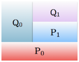
Figure 1: Decomposition of the solution space of the Boltzmann equation. The P₀ space is the kernel of the linearized collision operator, while the Q₀ space is spanned by excited mode, which is decomposed into the P₁ and Q₁ spaces.

Thus, we can reduce this requirement to the following two conditions;

• $\hat{L}\Psi$ and $Q_{0}F_{0}$ should belong to a common vector space.

• The P₁ space is spanned by independent components of $\hat{L}\Psi$ and $\Psi$.

The first condition is restated as that $\Psi$ and $\hat{L}^{-1}Q_{0}F_{0}$ should belong to a common vector space. Therefore let us calculate $\hat{L}^{-1}Q_{0}F_{0}$ and examine the structure of the vector space to which it belongs. This explicit calculation of the deformation of the distribution function constitutes one of the central parts of the present work, contrasting to the moment method in which some seemingly plausible ansatz is adopted without any explicit solution. A straightforward but somewhat tedious calculation of it is worked out in Appendix A: The result is given as

$$\big{[}\hat{L}^{-1}Q_{0}F_{0}\big{]}_{p} =\frac{1}{T}\Bigg{[}\big{[}\hat{L}^{-1}\hat{\Pi}\big{]}_{p}(-\nabla\cdot u)-\big{[}\hat{L}^{-1}\hat{J}^{\mu}\big{]}_{p}\frac{T}{h}\nabla_{\mu}\frac{\mu}{T}$$

$$+\big{[}\hat{L}^{-1}\hat{\pi}^{\mu\nu}\big{]}_{p}\Delta_{\mu\nu\rho\sigma}\nabla^{\rho}u^{\sigma}\Bigg{]}.$$ (60)

Here, $\hat{\Pi}_{p}$, $\hat{J}^{\mu}_{p}$, and $\hat{\pi}^{\mu\nu}_{p}$ are microscopic representations of dissipative currents whose definitions are given by

$$(\hat{\Pi}_{p},\hat{J}^{\mu}_{p},\hat{\pi}^{\mu\nu}_{p})=\frac{1}{p\cdot u}(\Pi_{p},J^{\mu}_{p},\pi^{\mu\nu}_{p}),$$ (61)

with

$$\Pi_{p} \equiv(p\cdot u)^{2}\Bigg{[}\frac{1}{3}-\left.\frac{\partial P}{\partial e}\right|_{n}\Bigg{]}+(p\cdot u)\left.\frac{\partial P}{\partial n}\right|_{e}-\frac{1}{3}m^{2},$$ (62)

$$J^{\mu}_{p} \equiv-\Delta^{\mu\nu}\,p_{\nu}((p\cdot u)-h),$$ (63)

$$\pi^{\mu\nu}_{p} \equiv\Delta^{\mu\nu\rho\sigma}\,p_{\rho}\,p_{\sigma}.$$ (64)

In the above equations, we have introduced the enthalpy per particle $h$ and the projection matrix $\Delta^{\mu\nu\rho\sigma}$ given by

$$h \equiv(e+P)/n,$$ (65)

$$\Delta^{\mu\nu\rho\sigma} \equiv 1/2(\Delta^{\mu\rho}\Delta^{\nu\sigma}+\Delta^{\mu\sigma}\Delta^{\nu\rho}-2/3\Delta^{\mu\nu}\Delta^{\rho\sigma}),$$ (66)

respectively. It is notable that the coefficients of the nine vectors $\big{[}\hat{L}^{-1}\,\hat{\Pi}\big{]}_{p}$, $\big{[}\hat{L}^{-1}\hat{J}^{\mu}\big{]}_{p}$, and $\big{[}\hat{L}^{-1}\hat{\pi}^{\mu\nu}\big{]}_{p}$ are linearly independent, i.e., the following statement is true;

$$\alpha(-T^{-1}\nabla\cdot u)+\beta^{\mu}(-h^{-1}\nabla_{\mu}(\mu/T))$$

$$+\gamma^{\mu\nu}(T^{-1}\Delta_{\mu\nu\rho\sigma}\nabla^{\rho}u^{\sigma})=0,\,\,\,\forall\,\,\,T,\,\mu,\,u^{\mu}$$

$$\rightarrow\alpha=\beta^{\mu}=\gamma^{\mu\nu}=0.$$ (67)

Thus, we can take the following nine vectors

$$\big{[}\hat{L}^{-1}\hat{\Pi}\big{]}_{p},\,\,\,\big{[}\hat{L}^{-1}\hat{J}^{\mu}\big{]}_{p},\,\,\,\big{[}\hat{L}^{-1}\hat{\pi}^{\mu\nu}\big{]}_{p},$$ (68)

as a set of the bases of the vector space that $\big{[}\hat{L}^{-1}Q_{0}F_{0}\big{]}_{p}$ and hence $\Psi$ belong to. Here we note that the above Lorentz vector and the tensor are transverse;

$$\big{[}\hat{L}^{-1}\hat{J}^{\mu}\big{]}_{p} =\Delta^{\mu\nu}\big{[}\hat{L}^{-1}\hat{J}_{\nu}\big{]}_{p},$$ (69)

$$\big{[}\hat{L}^{-1}\hat{\pi}^{\mu\nu}\big{]}_{p} =\Delta^{\mu\nu\rho\sigma}\big{[}\hat{L}^{-1}\hat{\pi}_{\rho\sigma}\big{]}_{p}.$$ (70)

Thus we now see that $\Psi$ can be written as a linear combination of these bases as

$$\Psi_{p} =\Bigg{[}\frac{\big{[}\hat{L}^{-1}\hat{\Pi}\big{]}_{p}}{\langle\hat{\Pi},\hat{L}^{-1}\hat{\Pi}{\rangle}}\Bigg{]}\Pi+\Bigg{[}\frac{h\big{[}\hat{L}^{-1}\hat{J}^{\mu}\big{]}_{p}}{\frac{1}{3}\langle\hat{J}^{\nu},\hat{L}^{-1}\hat{J}_{\nu}{\rangle}}\Bigg{]}J_{\mu}$$

$$+\Bigg{[}\frac{\big{[}\hat{L}^{-1}\hat{\pi}^{\mu\nu}\big{]}_{p}}{\frac{1}{5}\langle\hat{\pi}^{\rho\sigma},\hat{L}^{-1}\hat{\pi}_{\rho\sigma}{\rangle}}\Bigg{]}\pi_{\mu\nu}.$$ (71)

Here we have introduced the following nine vectors as mere coefficients of the basis vectors:

$$\Pi(\sigma;\tau_{0}),\,\,\,J^{\mu}(\sigma;\tau_{0}),\,\,\,\pi^{\mu\nu}(\sigma;\tau_{0}).$$ (72)

We stress that the form of $\Psi$ given in Eq. (III.1.2) is the most generic expression that makes $\hat{L}\Psi$ and $Q_{0}F_{0}$ belong to the common space.

As is clear now, we see that the P₁ space is identified with the vector space spanned by $\hat{\Pi}_{p}$, $\hat{J}^{\mu}_{p}$, $\hat{\pi}^{\mu\nu}_{p}$, $\big{[}\hat{L}^{-1}\hat{\Pi}\big{]}_{p}$, $\big{[}\hat{L}^{-1}\hat{J}^{\mu}\big{]}_{p}$, and $\big{[}\hat{L}^{-1}\hat{\pi}^{\mu\nu}\big{]}_{p}$. The sets of $\hat{\Pi}$ and $\hat{L}^{-1}\hat{\Pi}$, $\hat{J}^{\mu}$ and $\hat{L}^{-1}\hat{J}^{\mu}$, and $\hat{\pi}^{\mu\nu}$ and $\hat{L}^{-1}\hat{\pi}^{\mu\nu}$ are called the doublet modes Tsumura and Kunihiro (2013a). The Q₀ space is now decomposed into the P₁ space spanned by the doublet modes and the Q₁ space which is the complement to the P₀ and P₁ spaces. The corresponding projection operators are denoted as $P_{1}$ and $Q_{1}$, respectively.

Now we find that the coefficients $J^{\mu}$ and $\pi^{\mu\nu}$ in Eq. (III.1.2) are taken to be transverse without loss of generality; i.e.,

$$J^{\mu} =\Delta^{\mu\nu}J_{\nu},$$ (73)

$$\pi^{\mu\nu} =\Delta^{\mu\nu\rho\sigma}\pi_{\rho\sigma},$$ (74)

because of Eqs. (69) and (70). The properties (73) and (74) lead to the following identities:

$$u_{\mu}J^{\mu} =u_{\mu}\pi^{\mu\nu}=\Delta_{\mu\nu}\pi^{\mu\nu}=0,$$ (75)

$$\pi^{\mu\nu} =\pi^{\nu\mu}.$$ (76)

It will be found that $\Pi$, $J^{\mu}$, and $\pi^{\mu\nu}$ can be identified with the bulk pressure, thermal flux, and stress pressure, respectively.

The second-order equation is written as

$$\frac{\partial}{\partial\tau}\tilde{f}^{(2)}(\tau) =f^{\mathrm{eq}}\bar{f}^{\mathrm{eq}}\hat{L}(f^{\mathrm{eq}}\bar{f}^{\mathrm{eq}})^{-1}\tilde{f}^{(2)}(\tau)$$

$$+f^{\mathrm{eq}}\bar{f}^{\mathrm{eq}}K(\tau-\tau_{0}),$$ (77)

with the time-dependent inhomogeneous term given by

$$K(\tau-\tau_{0}) \equiv F_{1}\tilde{f}^{(1)}(\tau)+\frac{1}{2}B\Big{[}(f^{\mathrm{eq}}\bar{f}^{\mathrm{eq}})^{-1}\tilde{f}^{(1)}(\tau))\Big{]}^{2}$$

$$=F_{1}f^{\mathrm{eq}}\bar{f}^{\mathrm{eq}}\Big{[}\mathrm{e}^{\hat{L}(\tau-\tau_{0})}\Psi+(\tau-\tau_{0})P_{0}F_{0}$$

$$+(\mathrm{e}^{\hat{L}(\tau-\tau_{0})}-1)\hat{L}^{-1}Q_{0}F_{0}\Big{]}$$

$$+\frac{1}{2}B\Big{[}\mathrm{e}^{\hat{L}(\tau-\tau_{0})}\Psi+(\tau-\tau_{0})P_{0}F_{0}$$

$$+(\mathrm{e}^{\hat{L}(\tau-\tau_{0})}-1)\hat{L}^{-1}Q_{0}F_{0}\Big{]}^{2}.$$ (78)

Here, $F_{1}$ and $B$ are matrices and their components are given by

$$F_{1pq} \equiv-(f^{\mathrm{eq}}_{p}\bar{f}^{\mathrm{eq}}_{p})^{-1}\frac{1}{p\cdot u}p\cdot\nabla\delta_{pq},$$ (79)

$$B_{pqr} \equiv(f^{\mathrm{eq}}_{p}\bar{f}^{\mathrm{eq}}_{p})^{-1}\frac{1}{p\cdot u}\frac{\delta^{2}}{\delta f_{q}\delta f_{r}}C[f]_{p}\Bigg{|}_{f=f^{\mathrm{eq}}}f^{\mathrm{eq}}_{q}\bar{f}^{\mathrm{eq}}_{q}f^{\mathrm{eq}}_{r}\bar{f}^{\mathrm{eq}}_{r}.$$ (80)

In Eq. (III.1.2), we have used the notation

$$\big{[}B\psi\chi\big{]}_{p}=\int\mathrm{d}q\mathrm{d}rB_{pqr}\psi_{q}\chi_{r}.$$ (81)

The solution to Eq. (III.1.2) around $\tau\sim\tau_{0}$ is found to take the following form

$$\tilde{f}^{(2)}(\tau,\sigma;\tau_{0}) =f^{\mathrm{eq}}\bar{f}^{\mathrm{eq}}\Big{[}(\tau-\tau_{0})P_{0}$$

$$+(\tau-\tau_{0})(\hat{L}-\partial/\partial s)P_{1}\mathcal{G}(s)Q_{0}$$

$$-(1+(\tau-\tau_{0})\partial/\partial s)Q_{1}\mathcal{G}(s)Q_{0}\Big{]}\,K(s)\Big{|}_{s=0},$$ (82)

the initial value of which reads

$$f^{(2)}(\sigma;\tau_{0}) =\tilde{f}^{(2)}(\tau=\tau_{0},\sigma;\tau_{0})$$

$$=-f^{\mathrm{eq}}\bar{f}^{\mathrm{eq}}Q_{1}\mathcal{G}(s)Q_{0}K(s)\Big{|}_{s=0}.$$ (83)

The derivation of this solution is presented in Appendix B, where the complete expression of the solution not restricted to $\tau\sim\tau_{0}$ is given: In Eq. (III.1.2), we have retained only terms up to the first order of ($\tau-\tau_{0}$), and introduced a “propagator” defined by

$$\mathcal{G}(s)\equiv(\hat{L}-\partial/\partial s)^{-1}.$$ (84)

We notice again the appearance of secular terms in Eq. (III.1.2).

Summing up the perturbative solutions up to the second order with respect to $\epsilon$, we have the full expression of the approximate solution around $\tau\sim\tau_{0}$ to the second order:

$$\tilde{f}(\tau,\sigma;\tau_{0})$$

$$=f^{\mathrm{eq}}+\epsilon f^{\mathrm{eq}}\bar{f}^{\mathrm{eq}}\Big{[}(1+(\tau-\tau_{0})\hat{L})\Psi+(\tau-\tau_{0})F_{0}\Big{]}$$

$$+\epsilon^{2}f^{\mathrm{eq}}\bar{f}^{\mathrm{eq}}\Big{[}(\tau-\tau_{0})P_{0}+(\tau-\tau_{0})(\hat{L}-\partial/\partial s)P_{1}\mathcal{G}(s)Q_{0}$$

$$-(1+(\tau-\tau_{0})\partial/\partial s)Q_{1}\mathcal{G}(s)Q_{0}\Big{]}\,K(s)\Big{|}_{s=0},$$ (85)

with the initial value

$$f(\sigma;\tau_{0}) =f^{\mathrm{eq}}+\epsilon f^{\mathrm{eq}}\bar{f}^{\mathrm{eq}}\Psi$$

$$-\epsilon^{2}f^{\mathrm{eq}}\bar{f}^{\mathrm{eq}}Q_{1}\mathcal{G}(s)Q_{0}K(s)\Big{|}_{s=0}.$$ (86)

We note that the possible appearance of the fast motion caused by the Q₁ space in Eq. (III.1.2) is avoided by an appropriate choice of the initial value (III.1.2), as in the first-order solution; see Appendix B for the detail.

A couple of remarks are in order here:

1. In the present approach, we are solving the Boltzmann equation (1) as faithfully as possible, in contrast to the Israel-Stewart fourteen-moment method Israel and Stewart (1979), in which an ansatz for the solution is imposed in the form $f=f^{\mathrm{eq}}+\epsilon f^{\mathrm{eq}}\bar{f}^{\mathrm{eq}}\Psi^{\mathrm{14M}}$ with $\Psi^{\mathrm{14M}}=a+b^{\mu}p_{\mu}+c^{\mu\nu}p_{\mu}p_{\nu}$. Here, the coefficients $a$, $b^{\mu}$, and $c^{\mu\nu}$ are definite functions of $T$, $\mu$, $u^{\mu}$, $\Pi$, $J^{\mu}$, and $\pi^{\mu\nu}$ Israel and Stewart (1979). It is interesting that our initial value $\Psi$ given in Eq. (III.1.2) provides a foundation of the fourteen-moment method but with a novel form of $\Psi^{\mathrm{14M}}$.

2. Expanding $\mathcal{G}(s)Q_{0}$ in terms of $\hat{L}^{-1}{\partial}/{\partial s}$, the term $\mathcal{G}(s)Q_{0}K(s)|_{s=0}$ in Eqs. (III.1.2) and (III.1.2) is reduced to the form of infinite series as

   $$\mathcal{G}(s)Q_{0}K(s)\Big{|}_{s=0}$$

   $$=\sum_{n=0}^{\infty}\hat{L}^{-1-n}Q_{0}\frac{\partial^{n}}{\partial s^{n}}K(s)\Big{|}_{s=0},$$ (87)

   because $\partial^{n}K(s)/\partial s^{n}|_{s=0}$ does not vanish for any $n$; see Eq. (III.1.2). Admittedly the existence of such an infinite number of terms would be undesirable for the construction of the (closed) mesoscopic dynamics. It will be found, however, that an averaging procedure for obtaining the mesoscopic dynamics nicely leads to a cancellation of all the terms but single term in the resultant equation of motion thanks to the self-adjointness of $\hat{L}$ and the structure of the P₁ space spanned by the doublet modes; see Eq. (III.1.3) below.

III.1.3 RG improvement of perturbative expansion

We note that the solution (III.1.2) contains secular terms that apparently invalidate the perturbative expansion for $\tau$ away from the initial time $\tau_{0}$. The point of the RG method lies in the fact that we can utilize the secular terms to obtain an asymptotic solution valid in a global domain. Now we see that $\tilde{f}_{p}(\tau,\sigma;\tau_{0})$ in Eq. (III.1.2) provides a family of curves parameterized with $\tau_{0}$. They are all on the exact solution $f_{p}(\sigma;\tau)$ given by Eq. (III.1.2) at $\tau=\tau_{0}$ up to $O(\epsilon^{2})$, but only valid locally for $\tau$ near $\tau_{0}$. Thus, it is conceivable that the envelope of the family of curves, which is in contact with each local solution at $\tau=\tau_{0}$, will give a global solution in our asymptotic situation Kunihiro (1995, 1997); Ei et al. (2000); Hatta and Kunihiro (2002); Kunihiro and Tsumura (2006). According to the classical theory of envelopes, the envelope that is in contact with any curve in the family at $\tau=\tau_{0}$ is obtained by

$$\frac{\partial}{\partial\tau_{0}}\tilde{f}_{p}(\tau,\sigma;\tau_{0})\Bigg{|}_{\tau_{0}=\tau}=0,$$ (88)

where the subscript $p$ is restored for later convenience. Equation (88) is called the renormalization group equation Chen et al. (1994), and has also the meaning of the envelope equation Kunihiro (1995). We call Eq.(88) the RG/Envelope or RG/E equation following Kunihiro (1997). Now Eq.(88) is really reduced to

$$\frac{\partial}{\partial\tau}\Big{(}f^{\mathrm{eq}}(1+\epsilon\bar{f}^{\mathrm{eq}}\Psi)\Big{)}-\epsilon f^{\mathrm{eq}}\bar{f}^{\mathrm{eq}}\Big{[}\hat{L}\Psi+P_{0}F_{0}+Q_{0}F_{0}\Big{]}$$

$$-\epsilon^{2}f^{\mathrm{eq}}\bar{f}^{\mathrm{eq}}\Bigg{[}P_{0}+(\hat{L}-\partial/\partial s)P_{1}\mathcal{G}(s)Q_{0}$$

$$-(\partial/\partial s)\,Q_{1}\mathcal{G}(s)Q_{0}\Bigg{]}K(s)\Big{|}_{s=0}+O(\epsilon^{3})=0.$$ (89)

It is noted that Eq. (III.1.3) gives the equation of motion governing the dynamics of the would-be fourteen integral constants $T(\sigma;\tau)$, $\mu(\sigma;\tau)$, $u^{\mu}(\sigma;\tau)$, $\Pi(\sigma;\tau)$, $J^{\mu}(\sigma;\tau)$, and $\pi^{\mu\nu}(\sigma;\tau)$. The envelope function is given by the initial value (III.1.2) with the replacement of $\tau_{0}=\tau$ as

$$f^{\mathrm{G}}_{p}(\tau,\sigma) \equiv\tilde{f}_{p}(\tau,\sigma;\tau_{0}=\tau)$$

$$\equiv f_{p}(\sigma;\tau_{0}=\tau)$$

$$=f^{\mathrm{eq}}(1+\epsilon\bar{f}^{\mathrm{eq}}\Psi)$$

$$-\epsilon^{2}f^{\mathrm{eq}}\bar{f}^{\mathrm{eq}}Q_{1}\mathcal{G}(s)Q_{0}K(s)\Big{|}_{s=0}\Bigg{|}_{\tau_{0}=\tau}+O(\epsilon^{3}),$$ (90)

where the exact solution to the RG/E equation (III.1.3) is to be inserted. We note that the envelope function $f^{\mathrm{G}}_{p}(\tau,\sigma)$ is actually the global solution that solves the Boltzmann equation (III.1.1) up to $O(\epsilon^{2})$ in a global domain in the asymptotic regime: Indeed, for arbitrary $\tau(=\tau_{0})$ in the global domain in the asymptotic regime, we have

$$\frac{\partial}{\partial\tau}f^{\mathrm{G}}_{p}(\tau,\sigma) =\frac{\partial}{\partial\tau}\tilde{f}_{p}(\tau,\sigma;\tau_{0})\Bigg{|}_{\tau_{0}=\tau}+\frac{\partial}{\partial\tau_{0}}\tilde{f}_{p}(\tau,\sigma;\tau_{0})\Bigg{|}_{\tau_{0}=\tau}$$

$$=\frac{\partial}{\partial\tau}\tilde{f}_{p}(\tau,\sigma;\tau_{0})\Bigg{|}_{\tau_{0}=\tau},$$ (91)

where the RG/E equation (88) has been used. Furthermore, since $\tilde{f}_{p}(\tau,\sigma;\tau_{0})$ solves Eq. (III.1.1) with $\boldsymbol{a}^{\mu}(\sigma)=u^{\mu}(\sigma;\tau_{0})$ up to $O(\epsilon^{2})$, the r.h.s. of Eq. (III.1.3) reads

$$\frac{\partial}{\partial\tau}\tilde{f}_{p}(\tau,\sigma;\tau_{0}) =\frac{1}{p\cdot u(\sigma;\tau_{0})}C[\tilde{f}]_{p}(\tau,\sigma;\tau_{0})$$

$$-\epsilon\frac{1}{p\cdot u(\sigma;\tau_{0})}p^{\mu}\frac{\partial}{\partial\sigma^{\mu}}\tilde{f}_{p}(\tau,\sigma;\tau_{0})+O(\epsilon^{3}).$$ (92)

Then inserting the definition of $f^{\mathrm{G}}_{p}(\tau,\sigma)$ given in the first line of Eq. (III.1.3), we have

$$\frac{\partial}{\partial\tau}f_{p}^{\mathrm{G}}(\tau,\sigma) =\frac{1}{p\cdot u(\sigma;\tau)}C[f^{\mathrm{G}}]_{p}(\tau,\sigma)$$

$$-\epsilon\frac{1}{p\cdot u(\sigma;\tau)}p^{\mu}\frac{\partial}{\partial\sigma^{\mu}}f^{\mathrm{G}}_{p}(\tau,\sigma)+O(\epsilon^{3}).$$ (93)

This concludes the proof that the envelope function $f^{\mathrm{G}}_{p}(\tau,\sigma)$ is the global solution to the Boltzmann equation (III.1.1) up to $O(\epsilon^{2})$ in a global domain.

It is noteworthy that we have derived the mesoscopic dynamics of the relativistic Boltzmann equation (III.1.1) in the form of the pair of Eqs. (III.1.3) and (III.1.3). It is to be noted that an infinite number of terms, produced by $\mathcal{G}(s)$, are included both in the RG/E equation and the envelope function.

We observe that the RG/E equation (III.1.3) includes fast modes that should not be identified as the hydrodynamic modes even in the second order ones. While these modes could be incorporated to make a Langevnized hydrodynamic equation, we average out them to have the genuine hydrodynamic equation in the second order. This averaging can be made by taking the inner product of Eq. (III.1.3) with the zero modes $\varphi^{\alpha}_{0p}$ and the excited modes $\big{[}\hat{L}^{-1}(\hat{\Pi},\hat{J}^{\mu},\hat{\pi}^{\mu\nu})\big{]}_{p}$ used in the definition of $\Psi_{p}$. The first averaging leads to

$$\int\mathrm{d}p\varphi^{\alpha}_{0p}\Bigg{[}(p\cdot u)\frac{\partial}{\partial\tau}+\epsilon p\cdot\nabla\Bigg{]}\Bigg{[}f^{\mathrm{eq}}_{p}(1+\epsilon\bar{f}^{\mathrm{eq}}_{p}\Psi_{p})\Bigg{]}$$

$$=0+O(\epsilon^{3}),$$ (94)

and the second averaging

$$\int\mathrm{d}p\big{[}\hat{L}^{-1}(\hat{\Pi},\hat{J}^{\mu},\hat{\pi}^{\mu\nu})\big{]}_{p}\Bigg{[}(p\cdot u)\frac{\partial}{\partial\tau}$$

$$+\epsilon p\cdot\nabla\Bigg{]}\Bigg{[}f^{\mathrm{eq}}_{p}(1+\epsilon\bar{f}^{\mathrm{eq}}_{p}\Psi_{p})\Bigg{]}$$

$$=\epsilon\langle\hat{L}^{-1}(\hat{\Pi},\hat{J}^{\mu},\hat{\pi}^{\mu\nu}),\hat{L}\Psi\rangle$$

$$+\epsilon^{2}\frac{1}{2}\langle\hat{L}^{-1}(\hat{\Pi},\hat{J}^{\mu},\hat{\pi}^{\mu\nu}),B\Psi^{2}\rangle+O(\epsilon^{3}).$$ (95)

Here we have used the identity given by

$$\langle\hat{L}^{-1}(\hat{\Pi},\hat{J}^{\mu},\hat{\pi}^{\mu\nu}),(\hat{L}-\partial/\partial s)P_{1}\mathcal{G}(s)Q_{0}K(s)\Big{|}_{s=0}\rangle$$

$$=\langle(\hat{L}-\partial/\partial s)\hat{L}^{-1}(\hat{\Pi},\hat{J}^{\mu},\hat{\pi}^{\mu\nu}),P_{1}\mathcal{G}(s)Q_{0}K(s)\Big{|}_{s=0}\rangle$$

$$=\langle(\hat{L}-\partial/\partial s)\hat{L}^{-1}(\hat{\Pi},\hat{J}^{\mu},\hat{\pi}^{\mu\nu}),\mathcal{G}(s)Q_{0}K(s)\Big{|}_{s=0}\rangle$$

$$=\langle\hat{L}^{-1}(\hat{\Pi},\hat{J}^{\mu},\hat{\pi}^{\mu\nu}),(\hat{L}-\partial/\partial s)\mathcal{G}(s)Q_{0}K(s)\Big{|}_{s=0}\rangle$$

$$=\langle\hat{L}^{-1}(\hat{\Pi},\hat{J}^{\mu},\hat{\pi}^{\mu\nu}),Q_{0}K(s)\Big{|}_{s=0}\rangle$$

$$=\langle\hat{L}^{-1}(\hat{\Pi},\hat{J}^{\mu},\hat{\pi}^{\mu\nu}),K(0)\rangle$$

$$=\langle\hat{L}^{-1}(\hat{\Pi},\hat{J}^{\mu},\hat{\pi}^{\mu\nu}),F_{1}f^{\mathrm{eq}}\bar{f}^{\mathrm{eq}}\Psi\rangle$$

$$+\frac{1}{2}\langle\hat{L}^{-1}(\hat{\Pi},\hat{J}^{\mu},\hat{\pi}^{\mu\nu}),B\Psi^{2}\rangle,$$ (96)

where utilized are the self-adjointness of $\hat{L}_{pq}$ shown in Eq. (III.1.2), the structure of the P₁ space spanned by the doublet modes, i.e., the pairs of $\hat{\Pi}_{p}$ and $\big{[}\hat{L}^{-1}\hat{\Pi}\big{]}_{p}$, $\hat{J}^{\mu}_{p}$ and $\big{[}\hat{L}^{-1}\hat{J}^{\mu}\big{]}_{p}$, and $\hat{\pi}^{\mu\nu}_{p}$ and $\big{[}\hat{L}^{-1}\hat{\pi}^{\mu\nu}\big{]}_{p}$, and the equality $K(0)=F_{1}f^{\mathrm{eq}}\bar{f}^{\mathrm{eq}}\Psi+B\Psi^{2}/2$ derived from Eq. (III.1.2).

Thus the pair of Eqs. (III.1.3) and (III.1.3) constitutes the hydrodynamic equation in the second order, i.e., the equation of motion governing $T$, $\mu$, $u^{\mu}$, $\Pi$, $J^{\mu}$, and $\pi^{\mu\nu}$. It is to be noted that this pair of equations is free from an infinite number of terms in contrast to the RG/E equation (III.1.3) and much simpler than it. We stress that this simplification through the averaging by $\hat{L}^{-1}(\hat{\Pi},\hat{J}^{\mu},\hat{\pi}^{\mu\nu})$ is due to the self-adjointness of $\hat{L}$ and the structure of the P₁ space spanned by the doublet modes $(\hat{\Pi},\hat{J}^{\mu},\hat{\pi}^{\mu\nu})$ and $\hat{L}^{-1}(\hat{\Pi},\hat{J}^{\mu},\hat{\pi}^{\mu\nu})$.

III.2 Properties of the reduced dynamics

We now put back to $\epsilon=1$. Noting that $(p\cdot u)\frac{\partial}{\partial\tau}+p\cdot\nabla=p^{\mu}\partial_{\mu}$, we find that Eq. (III.1.3) finally takes the following form

$$\partial_{\mu}J^{\mu\alpha}_{\mathrm{hydro}}=0,$$ (97)

with

$$J^{\mu\alpha}_{\mathrm{hydro}} \equiv\int\mathrm{d}pp^{\mu}\varphi^{\alpha}_{0p}f^{\mathrm{eq}}_{p}(1+\bar{f}^{\mathrm{eq}}_{p}\Psi_{p})$$

$$=\left\{\begin{array}[]{ll}\displaystyle{eu^{\mu}u^{\nu}-(P+\Pi)\Delta^{\mu\nu}+\pi^{\mu\nu},}&\displaystyle{\alpha=\nu,}\\[5.69054pt] \displaystyle{nu^{\mu}+J^{\mu},}&\displaystyle{\alpha=4.}\end{array}\right.$$ (100)

We remark that Eq. (97) is nothing but the balance equations and $J^{\mu\nu}_{\mathrm{hydro}}$ and $J^{\mu 4}_{\mathrm{hydro}}$ can be identified with the energy-momentum tensor $T^{\mu\nu}$ and particle current $N^{\mu}$ in the Landau-Lifshitz frame, respectively. Indeed, we can derive the same expression as $J^{\mu\alpha}_{\mathrm{hydro}}$ by substituting the distribution function $f^{\mathrm{G}}(\tau,\sigma)$ in Eq. (III.1.3) into the definitions of $T^{\mu\nu}$ and $N^{\mu}$ given by Eqs. (12) and (11).

After a straightforward manipulation whose details are presented in Appendix C, we can reduce Eq. (III.1.3) into the following relaxation equations:

$$\Pi =-\zeta\theta$$

$$-\tau_{\Pi}\frac{\partial}{\partial\tau}\Pi-\ell_{\Pi J}\nabla\cdot J$$

$$+\kappa_{\Pi\Pi}\Pi\theta$$

$$+\kappa^{(1)}_{\Pi J}J_{\rho}\nabla^{\rho}T+\kappa^{(2)}_{\Pi J}J_{\rho}\nabla^{\rho}\frac{\mu}{T}$$

$$+\kappa_{\Pi\pi}\pi_{\rho\sigma}\sigma^{\rho\sigma}$$

$$+b_{\Pi\Pi\Pi}\Pi^{2}+b_{\Pi JJ}J^{\rho}J_{\rho}+b_{\Pi\pi\pi}\pi^{\rho\sigma}\pi_{\rho\sigma},$$ (101)

$$J^{\mu} =\lambda\frac{T^{2}}{h^{2}}\nabla^{\mu}\frac{\mu}{T}$$

$$-\tau_{J}\Delta^{\mu\rho}\frac{\partial}{\partial\tau}J_{\rho}-\ell_{J\Pi}\nabla^{\mu}\Pi-\ell_{J\pi}\Delta^{\mu\rho}\nabla_{\nu}{\pi^{\nu}}_{\rho}$$

$$+\kappa^{(1)}_{J\Pi}\Pi\nabla^{\mu}T+\kappa^{(2)}_{J\Pi}\Pi\nabla^{\mu}\frac{\mu}{T}$$

$$+\kappa^{(1)}_{JJ}J^{\mu}\theta+\kappa^{(2)}_{JJ}J_{\rho}\sigma^{\mu\rho}+\kappa^{(3)}_{JJ}J_{\rho}\omega^{\mu\rho}$$

$$+\kappa^{(1)}_{J\pi}\pi^{\mu\rho}\nabla_{\rho}T+\kappa^{(2)}_{J\pi}\pi^{\mu\rho}\nabla_{\rho}\frac{\mu}{T}$$

$$+b_{J\Pi J}\Pi J^{\mu}+b_{JJ\pi}J_{\rho}\pi^{\rho\mu},$$ (102)

$$\pi^{\mu\nu} =2\eta\sigma^{\mu\nu}$$

$$-\tau_{\pi}\Delta^{\mu\nu\rho\sigma}\frac{\partial}{\partial\tau}\pi_{\rho\sigma}-\ell_{\pi J}\nabla^{\langle\mu}J^{\nu\rangle}$$

$$+\kappa_{\pi\Pi}\Pi\sigma^{\mu\nu}$$

$$+\kappa^{(1)}_{\pi J}J^{\langle\mu}\nabla^{\nu\rangle}T+\kappa^{(2)}_{\pi J}J^{\langle\mu}\nabla^{\nu\rangle}\frac{\mu}{T}$$

$$+\kappa^{(1)}_{\pi\pi}\pi^{\mu\nu}\theta+\kappa^{(2)}_{\pi\pi}{\pi_{\rho}}^{\langle\mu}\sigma^{\nu\rangle\rho}+\kappa^{(3)}_{\pi\pi}{\pi_{\rho}}^{\langle\mu}\omega^{\nu\rangle\rho}$$

$$+b_{\pi\Pi\pi}\Pi\pi^{\mu\nu}+b_{\pi JJ}J^{\langle\mu}J^{\nu\rangle}+b_{\pi\pi\pi}\pi^{\lambda\langle\mu}{\pi^{\nu\rangle}}_{\lambda},$$ (103)

where we have introduced the notation $A^{\langle\mu\nu\rangle}\equiv\Delta^{\mu\nu\rho\sigma}A_{\rho\sigma}$ for a traceless and symmetric tensor. Here $\theta\equiv\nabla\cdot u$, $\sigma^{\mu\nu}\equiv\Delta^{\mu\nu\rho\sigma}\nabla_{\rho\sigma}$, and $\omega^{\mu\nu}\equiv\frac{1}{2}(\nabla^{\mu}u^{\nu}-\nabla^{\mu}u^{\nu})$ denote the scalar expansion, shear tensor and vorticity, respectively. We refer to Appendix C for the explicit definitions of many other hydrodynamic valuables introduced in (III.2)-(III.2).

Now the physical meaning of each term in (III.2)-(III.2) should be clear: The first lines in Eqs. (III.2)-(III.2) are identical with the so-called constitutive equations, which define the relations between the dissipative variables $\Pi$, $J^{\mu}$, and $\pi^{\mu\nu}$ and the thermodynamic forces given by the gradients of $T$, $\mu$, and $u^{\mu}$. Substituting the constitutive equations into the conserved currents $J^{\mu\alpha}_{\mathrm{hydro}}$ in Eq. (III.2), we have the first-order hydrodynamics in the Landau-Lifshitz frame. The terms in the other lines are the new terms appearing in the second-order hydrodynamics. The second lines denote the relaxation terms given by the temporal and spatial derivatives of the dissipative variables, which describe the relaxation processes of the dissipative variables to the thermodynamic forces. The third, fourth, and fifth lines are composed of the products of the thermodynamic forces and dissipative variables, among which we remark that the vorticity term appears. The final lines give the non-linear terms of the dissipative variables.

Our approach is based on a kind of statistical physics, and thus give microscopic expressions of the transport and relaxation coefficeints. Here we present the resultant microscopic representations of the transport coefficients , i.e., the bulk viscosity $\zeta$, thermal conductivity $\lambda$, and shear viscosity $\eta$, and some of the relaxation times $\tau_{\Pi}$, $\tau_{J}$, and $\tau_{\pi}$;

$$\zeta =-\frac{1}{T}\langle\hat{\Pi},\hat{L}^{-1}\hat{\Pi}\rangle\equiv\zeta^{\mathrm{RG}},$$ (104)

$$\lambda =\frac{1}{3T^{2}}\langle\hat{J}^{\mu},\hat{L}^{-1}\hat{J}_{\mu}\rangle\equiv\lambda^{\mathrm{RG}},$$ (105)

$$\eta =-\frac{1}{10T}\langle\hat{\pi}^{\mu\nu},\hat{L}^{-1}\hat{\pi}_{\mu\nu}\rangle\equiv\eta^{\mathrm{RG}},$$ (106)

$$\tau_{\Pi} =-\frac{\langle\hat{\Pi},\hat{L}^{-2}\hat{\Pi}\rangle}{\langle\hat{\Pi},\hat{L}^{-1}\hat{\Pi}\rangle}\equiv\tau^{\mathrm{RG}}_{\Pi},$$ (107)

$$\tau_{J} =-\frac{\langle\hat{J}^{\mu},\hat{L}^{-2}\hat{J}_{\mu}\rangle}{\langle\hat{J}^{\rho},\hat{L}^{-1}\hat{J}_{\rho}\rangle}\equiv\tau^{\mathrm{RG}}_{J},$$ (108)

$$\tau_{\pi} =-\frac{\langle\hat{\pi}^{\mu\nu},\hat{L}^{-2}\hat{\pi}_{\mu\nu}\rangle}{\langle\hat{\pi}^{\rho\sigma},\hat{L}^{-1}\hat{\pi}_{\rho\sigma}\rangle}\equiv\tau^{\mathrm{RG}}_{\pi}.$$ (109)

We leave the microscopic expressions of other coefficients in Appendix C. We first note that $\zeta^{\mathrm{RG}}$, $\lambda^{\mathrm{RG}}$, and $\eta^{\mathrm{RG}}$ are perfectly in agreement with those of the Chapman-Enskog (CE) expansion method de Groot et al. (1980), which we denote as $\zeta^{\mathrm{CE}}$, $\lambda^{\mathrm{CE}}$, and $\eta^{\mathrm{CE}}$. Here it is noteworthy that our expressions of the transport coefficients can be nicely rewritten in the form of Green-Kubo formula Jeon (1995); Jeon and Yaffe (1996); Hidaka and Kunihiro (2011) in the linear response theory. To see this, we first introduce the “time-evolved” vectors defined by

$$(\hat{\Pi}_{p}(s),\hat{J}^{\mu}_{p}(s),\hat{\pi}^{\mu\nu}_{p}(s))\equiv\int\mathrm{d}q\big{[}\mathrm{e}^{s\hat{L}}\big{]}_{pq}(\hat{\Pi}_{q},\hat{J}^{\mu}_{q},\hat{\pi}^{\mu\nu}_{q}),$$ (110)

where the time-evolution operator is given by the linearized collision operator. Then, we have

$$\zeta^{\mathrm{RG}} =\frac{1}{T}\int_{0}^{\infty}\mathrm{d}s\langle\hat{\Pi}(0),\hat{\Pi}(s)\rangle,$$ (111)

$$\lambda^{\mathrm{RG}} =-\frac{1}{3T^{2}}\int_{0}^{\infty}\mathrm{d}s\langle\hat{J}^{\mu}(0),\hat{J}_{\mu}(s)\rangle,$$ (112)

$$\eta^{\mathrm{RG}} =\frac{1}{10T}\int_{0}^{\infty}\mathrm{d}s\langle\hat{\pi}^{\mu\nu}(0),\hat{\pi}_{\mu\nu}(s)\rangle.$$ (113)

We note that the integrands in the formulae have the meanings of the relaxation functions or time correlation functions;

$$R_{\Pi}(s) \equiv\frac{1}{T}\langle\hat{\Pi}(0),\hat{\Pi}(s)\rangle,$$ (114)

$$R_{J}(s) \equiv-\frac{1}{3T^{2}}\langle\hat{J}^{\mu}(0),\hat{J}_{\mu}(s)\rangle,$$ (115)

$$R_{\pi}(s) =\frac{1}{10T}\langle\hat{\pi}^{\mu\nu}(0),\hat{\pi}_{\mu\nu}(s)\rangle.$$ (116)

We stress that the results of the transport coefficients all show the reliability of our approach based on the doublet scheme in the RG method. We remark that the naive version of moment method by Israel and Stewart (IS) fails to give the Chapman-Enskog formulae Israel and Stewart (1979), as is well known.

Thus it may be a good news for us that the explicit formulae of the relaxation times given above also differ from those given by IS Israel and Stewart (1979), which read

$$\tau_{\Pi}^{\mathrm{IS}} \equiv-\frac{\langle\Pi,\Pi\rangle}{\langle\Pi,\hat{L}\Pi\rangle},$$ (117)

$$\tau_{J}^{\mathrm{IS}} \equiv-\frac{\langle\,J^{\mu},J_{\mu}\rangle}{\langle J^{\rho},\hat{L}J_{\rho}\rangle},$$ (118)

$$\tau_{\pi}^{\mathrm{IS}} \equiv-\frac{\langle\pi^{\mu\nu},\pi_{\mu\nu}\rangle}{\langle\pi^{\rho\sigma},\hat{L}\pi_{\rho\sigma}\rangle}.$$ (119)

Indeed we shall now show that our formulae of the relaxation times allow a natural interpretation of them. To see this, we rewrite the expressions of the relaxation times given in Eqs. (107)-(109) in terms of the time-evolved vectors again:

$$\tau^{\mathrm{RG}}_{\Pi} =\frac{\int_{0}^{\infty}\mathrm{d}s\,sR_{\Pi}(s)}{\int_{0}^{\infty}\mathrm{d}sR_{\Pi}(s)},$$ (120)

$$\tau^{\mathrm{RG}}_{J} =\frac{\int_{0}^{\infty}\mathrm{d}s\,sR_{J}(s)}{\int_{0}^{\infty}\mathrm{d}sR_{J}(s)},$$ (121)

$$\tau^{\mathrm{RG}}_{\pi} =\frac{\int_{0}^{\infty}\mathrm{d}s\,sR_{\pi}(s)}{\int_{0}^{\infty}\mathrm{d}sR_{\pi}(s)}.$$ (122)

It is noteworthy that all the relaxation times are expressed in terms of the relaxation functions $R_{\Pi}(s)$, $R_{J}(s)$, and $R_{\pi}(s)$, respectively. Then the formulae (120)-(122) allow the natural interpretation of the resepective relaxation times as the correlation times in the respective relaxation functions. We emphasize that it is for the first time that the relaxation times are expressed in terms of the relaxation functions in the context of the derivation of the second-order relativistic hydrodynamic equation from the relativistic Boltzmann equation.

III.3 Discussions

We now examine the basic properties of the resultant hydrodynamic equations (97) and (III.2)-(III.2). First we show that our equation is really causal in the sense that the velocities of any fluctuation around the equilibrium is less than that of the light velocity with a detailed proof is left to Appendix D, where the stability of the static solution is also prooved. Next we compare our formulae of the relaxation equations with those derived by the moment method. Then we give numerical results of the transport coefficients and relaxation times given by Eqs. (104)-(106) and (107)-(109), respectively, and compare them with those by other methods.

III.3.1 Causal property of hydrodynamic equations obtained by RG method

We give a brief account of the proof that the velocities of hydrodynamic modes described by the hydrodynamic equations (97) and (III.2)-(III.2) do not exceed the speed of light, i.e., the unity. We note that the detailed proof is presented in Appendix D.

First, we linearize the hydrodynamic equations around equilibrium state specified by constant temperature, constant chemical potential, and constant fluid flow, as follows:

$$(\Lambda\,A^{\alpha\beta,\gamma\delta}-\tilde{B}^{\alpha\beta,\gamma\delta}(k))\,\delta\tilde{X}_{\gamma\delta}(\Lambda\,;\,k)=0,$$ (123)

where the matrices $A^{\alpha\beta,\gamma\delta}$ and $\tilde{B}^{\alpha\beta,\gamma\delta}(k)$ are defined in Eqs. (25)-(28) and (35)-(38), respectively, and the variables $\delta\tilde{X}_{\alpha\beta}(\Lambda\,;\,k)$ are Fourier-Laplace transformations of $\delta X_{\alpha\beta}(\tau\,;\,\sigma)$ given by

$$\delta X_{\mu\nu} \equiv \frac{\Delta_{\mu\nu}}{3\,T\,\zeta^{\mathrm{RG}}}\Bigg{|}_{\mathrm{eq}}\,\delta\Pi-\frac{1}{2\,T\,\eta^{\mathrm{RG}}}\Bigg{|}_{\mathrm{eq}}\,\delta\pi_{\mu\nu},$$ (124)

$$\delta X_{\mu 4} \equiv \frac{h}{T^{2}\,\lambda^{\mathrm{RG}}}\Big{|}_{\mathrm{eq}}\,\delta J_{\mu},$$ (125)

$$\delta X_{4\mu} \equiv -\frac{1}{T}\Big{|}_{\mathrm{eq}}\,\delta u_{\mu}+\frac{u_{\mu}}{T^{2}}\Big{|}_{\mathrm{eq}}\,\delta T,$$ (126)

$$\delta X_{44} \equiv \frac{1}{T}\Big{|}_{\mathrm{eq}}\,\delta\mu-\frac{\mu}{T^{2}}\Big{|}_{\mathrm{eq}}\,\delta T,$$ (127)

with the arguments $(\tau\,;\,\sigma)$ being omitted. Here, $\delta T$, $\delta\mu$, $\delta u^{\mu}$, $\delta\Pi$, $\delta J^{\mu}$, and $\delta\pi^{\mu\nu}$ are fluctuations from the equilibrium state and all coefficients take values at the equilibrium state. Furthermore, $i\Lambda$ and $k^{\mu}$ are frequency and wavelength conjugate to $\tau$ and $\sigma^{\mu}$, respectively. We note that $k^{\mu}$ is space-like vector, $k^{2}<0$, for any $k^{\mu}\neq 0$, which satisfies $k^{\mu}=\Delta^{\mu\nu}k_{\nu}$ because of $\sigma^{\mu}=\Delta^{\mu\nu}\sigma_{\nu}$. We also note that the condition $\delta\tilde{X}\neq 0$ into Eq. (123) leads to the dispersion relation $\Lambda=\Lambda(k)$.

Then, as a typical quantity used for the check of the causality, we examine a character velocity $v_{\mathrm{ch}}$ that is defined as

$$v_{\mathrm{ch}}\equiv\lim_{-k^{2}\rightarrow\infty}\,\sqrt{\frac{\partial}{\partial k_{\mu}}\Lambda(k)\cdot\frac{\partial}{\partial k^{\mu}}\Lambda(k)}.$$ (128)

With the use of the explicit definitions of $A^{\alpha\beta,\gamma\delta}$ and $\tilde{B}^{\alpha\beta,\gamma\delta}(k)$, we can show that

$$v_{\mathrm{ch}}\leq 1,$$ (129)

is satisfied for any collision operator $\hat{L}_{pq}$, that is, any differential cross section. We emphasize that our hydrodynamic equations surely have the causal property, and hence can be applied to various high-energy hydrodynamic systems.

III.3.2 Relation between relaxation equations by RG method and those by the other formalisms

The relaxation equations (III.2)-(III.2) can be made into the different form by iteration. Here, let us focus on the relaxation equation for the stress tensor, i.e., Eq. (III.2), by setting $\Pi=J^{\mu}=0$:

$$\pi^{\mu\nu} =2\eta^{\mathrm{RG}}\sigma^{\mu\nu}-\tau^{\mathrm{RG}}_{\pi}\Delta^{\mu\nu\rho\sigma}\frac{\partial}{\partial\tau}\pi_{\rho\sigma}+b_{\pi\pi\pi}\pi^{\lambda\langle\mu}{\pi^{\nu\rangle}}_{\lambda}$$

$$+\kappa^{(1)}_{\pi\pi}\pi^{\mu\nu}\theta+\kappa^{(2)}_{\pi\pi}{\pi_{\rho}}^{\langle\mu}\sigma^{\nu\rangle\rho}+\kappa^{(3)}_{\pi\pi}{\pi_{\rho}}^{\langle\mu}\omega^{\nu\rangle\rho}.$$ (130)

By solving this equation with respect to $\pi^{\mu\nu}$ in an iterative manner and using the equality

$$\Delta^{\mu\nu\rho\sigma}\frac{\partial}{\partial\tau}\sigma_{\rho\sigma} =-\frac{\partial}{\partial\tau}u^{\langle\mu}\cdot\frac{\partial}{\partial\tau}u^{\nu\rangle}+\nabla^{\langle\mu}\frac{\partial}{\partial\tau}u^{\nu\rangle}-\frac{2}{3}\theta\sigma^{\mu\nu}$$

$$-\sigma^{\lambda\langle\mu}{\sigma^{\nu\rangle}}_{\lambda}-\omega^{\lambda\langle\mu}{\omega^{\nu\rangle}}_{\lambda}-2\sigma^{\lambda\langle\mu}{\omega^{\nu\rangle}}_{\lambda},$$ (131)

and the balance equation (97), we find that the resultant equation includes the following terms

$$\sigma^{\lambda\langle\mu}{\sigma^{\nu\rangle}}_{\lambda},\,\,\,\omega^{\lambda\langle\mu}{\omega^{\nu\rangle}}_{\lambda},\,\,\,\sigma^{\lambda\langle\mu}{\omega^{\nu\rangle}}_{\lambda},\,\,\,\theta\sigma^{\mu\nu},$$

$$\nabla^{\langle\mu}T\cdot\nabla^{\nu\rangle}T,\,\,\,\nabla^{\langle\mu}T\cdot\nabla^{\nu\rangle}\frac{\mu}{T},\,\,\,\nabla^{\langle\mu}\frac{\mu}{T}\cdot\nabla^{\nu\rangle}\frac{\mu}{T},$$

$$\nabla^{\langle\mu}\nabla^{\nu\rangle}T,\,\,\,\nabla^{\langle\mu}\nabla^{\nu\rangle}\frac{\mu}{T},$$ (132)

in addition to those given in Eq. (III.3.2). In this iterative manner, our hydrodynamic equation apparently gets to have all the terms given by $\mathcal{K}^{\mu\nu}$ of Eq. (73) in Denicol et al. (2012b). Notice, however, that the last two terms of Eq. (III.3.2) have a form of the second-order spatial derivatives of hydrodynamic variables, which make the hydrodynamic equation parabolic and accordingly acausal. Hence, we have an important observation that the naive iteration may spoil the causal property of the original hydrodynamic equation, and thus we must use the original form of the relaxation equations (III.3.2) or (III.2)-(III.2). Furthermore, since the appearance of the nonlinear vortex term $\omega^{\lambda\langle\mu}{\omega^{\nu\rangle}}_{\lambda}$ seems to be inevitably associated with that of the second-order spatial derivative terms, the explicit appearance of such a nonlinear vortex term should be avoided in the relaxation equation although its effect should be included in Eq. (III.3.2) implicitly.

III.3.3 Numerical example: transport coefficients and relaxation times

In this subsection, we present numerical examples of the transport coefficients and relaxation times using the microscopic expressions given in the present approach, and compare them with those in the previous works. Note that the microscopic expressions are solely given in terms of the linearized collision operator $\hat{L}$, which is in turn uniquely determined by the transition probability $\omega(p\,,\,p_{1}|p_{2}\,,\,p_{3})$. A general form of the transition probability reads

$$\omega(p\,,\,p_{1}|p_{2}\,,\,p_{3})=\delta^{4}(p+p_{1}-p_{2}-p_{3})\,s\,\sigma(s,\,\theta),$$ (133)

where $\sigma(s,\,\theta)$ denotes a differential cross section, $s\equiv(p+p_{1})^{2}$ a total momentum squared, and $\theta\equiv\cos^{-1}[(p-p_{1})\cdot(p_{2}-p_{3})/(p-p_{1})^{2}]$ a scattering angle. Here, we examine the case of a constant cross section for simplicity;

$$\sigma(s,\,\theta)=\sigma_{T}/4\pi$$ (134)

with $\sigma_{T}$ being a total cross section.

We focus on the shear viscosity $\eta$ and relaxation time $\tau_{\pi}$ for the stress tensor in the classical and massless limits, i.e., $a=0$ and $m/T=0$. The calculation of $\eta$ and $\tau_{\pi}$ can be reduced to that of $X_{p}\equiv\big{[}\hat{L}^{-1}\hat{\pi}^{\mu\nu}\big{]}_{p}$, which satisfies the linear equation $\big{[}\hat{L}X\big{]}_{p}=\hat{\pi}^{\mu\nu}_{p}$. The last equation can be solved numerically in an exact manner without recourse to any ansatz for the functional form of $X_{p}$.

In Table 1, we show the numerical results together with those of the previous works. We confirm that our formulae for $\eta$ and $\tau_{\pi}$ give results different from those by the (naive) Israel-Stewart moment method Israel and Stewart (1979). Furthermore, our relaxation time differs from that of Denicol et al. Denicol et al. (2012b), which is an improvement of the Israel-Stewart moment method adopting 41 moments, although their result for the shear viscosity tends to numerically agrees with the Chapman-Enskog/RG value de Groot et al. (1980).

Table 1: Values of the shear viscosity and relaxation time for the stress tensor for a classical gas with a constant cross section in the massless limit, in the RG method, Israel-Stewart’s 14-moment method Israel and Stewart (1979), and Denicol et al.’s 41-moment method Denicol et al. (2012b).

	RG	Israel-Stewart	Denicol et al.
$\eta$ [$T/\sigma_{T}$]	1.27	1.2	1.267
$\tau_{\pi}$ [$1/n\sigma_{T}$]	1.66	1.8	2

IV Summary and concluding remarks

In this paper, we have derived the second-order hydrodynamic equation systematically from the relativistic Boltzmann equation with the quantum statistical effect. Our derivation is based on a novel development of the renormalization-group (RG) method. In this method, we have solved the Boltzmann equation faithfully in a way valid up to the mesoscopic scales of space and time, and then have reduced the solution to a simpler equation describing the mesoscopic dynamics of the Boltzmann equation. We have found that our theory nicely gives a compact expression of the deviation of the distribution function in terms of the linearized collision operator, which is different from those used as an ansatz in the conventional fourteen-moment method. In fact, in contrast to the ansatz in the fourteen-moment method, our distribution function produces the transport coefficients which have the same microscopic expressions as those derived in the Chapman-Enskog expansion method. Furthermore, new microscopic expressions of the relaxation times are obtained, which differ from those derived in any other formalisms such as the moment method. We have shown that the present expressions of the relaxation times can be nicely rewritten in terms of the respective relaxation functions, which allow a physically natural interpretation of the relaxation times, and thus assert the plausibility of our results.

The present asymptotic analysis utilizing a perturbation theory is based on the physical assumption that only the spatial inhomogeneity is the origin of the dissipation, and the expansion parameter $\epsilon$ is introduced for characterizing the inhomogeneity, which may be identified with the Knudsen number: The inhomogeneity gives a deviation of the distribution function from the local equilibrium one $f^{\rm eq}$, and accordingly the ratio of the deviation to $f^{\rm eq}$ is necessarily proportional to $\epsilon$. We emphasize that the inhomogeneity and the ratio of the distribution functions are necessarily of the same order in our asymptotic analysis. It is worth emphasizing that the present asymptotic analysis combined with the perturbative expansion successfully solves the Boltzmann equation consistently and leads to the mesoscopic dynamics including the constitutive equations that relate the dissipative quantities and the spatial gradients of the equilibrium quantities.

We have given a proof that the propagating velocities of the fluctuations of the hydrodynamical variables do not exceed the light velocity, and hence our seconder-order equation ensures the desired causality. We have also proved that the equilibrium state is stable for any perturbation described by our equation. These results strongly suggest the validity of our formulation based on the RG method.

We have demonstrated numerically that the relaxation times differ from those given in the moment methods in the literature, even in the sophisticated one so as to numerically reproduce the transport coefficients given in the Chapman-Enskog (and RG) method. The calculation was done only in the case of a constant differential cross section. It is interesting to extend the present calculation to more realistic cases with the differential cross section depending on the total momentum and scattering angle, which have immediate applications to relativistic systems consisting of quarks, gluons, and hadrons. Then it is an imperative task to apply the present method to derive the multi-component relativistic hydrodynamic equation, which is now under way Kikuchi et al. . It is of interest to use the resultant equations for phenomenological analysis of relativistic heavy-ion collisions performed in RHIC and LHC, although there exist multi-component hydrodynamic equations deriven on the basis of the moment method Prakash et al. (1993); Monnai and Hirano (2010), which was found to have unsatisfactory aspects for the single-component equation, as was shown in the present article.

Appendix A Detailed derivation of the excited modes and their explicit expressions

In this Appendix, we derive the expression of Eq.(III.1.2), whose calculation can be reduced to that of

$$\big{[}Q_{0}F_{0}\big{]}_{p}=\big{[}F_{0}-P_{0}F_{0}\big{]}_{p}=F_{0p}-\varphi_{0p}^{\alpha}\eta^{-1}_{0\alpha\beta}\langle\varphi_{0}^{\beta},F_{0}\rangle,$$ (1)

with

$$F_{0p}=\frac{1}{p\cdot u}\Bigg{[}p^{\mu}p^{\nu}\nabla_{\mu}\frac{u_{\nu}}{T}-p^{\mu}\nabla_{\mu}\frac{\mu}{T}\Bigg{]}.$$ (2)

Here, we have used Eq. (44) and $f^{\mathrm{eq}}_{p}=1/[\mathrm{e}^{(p\cdot u-\mu)/T}-a]$.

We introduce the following quantities for later covenience:

$$a_{\ell}\equiv\int\mathrm{d}pf^{\mathrm{eq}}_{p}\bar{f}^{\mathrm{eq}}_{p}(p\cdot u)^{\ell},\,\,\,\ell=0,\,1,\,\cdots.$$ (3)

Then the metric $\eta^{\alpha\beta}_{0}=\langle\varphi_{0}^{\alpha},\varphi_{0}^{\beta}\rangle$ are expressed as

$$\eta^{\mu\nu}_{0} =a_{3}u^{\mu}u^{\nu}+(m^{2}a_{1}-a_{3})\frac{1}{3}\Delta^{\mu\nu},$$ (4)

$$\eta^{\mu 4}_{0}=\eta^{4\mu}_{0} =a_{2}u^{\mu},$$ (5)

$$\eta^{44}_{0} =a_{1},$$ (6)

while the inverse metric $\eta_{0\alpha\beta}^{-1}$ read

$$\eta^{-1}_{0\mu\nu} =\frac{a_{1}u^{\mu}u^{\nu}}{a_{3}a_{1}-a^{2}_{2}}+\frac{3\Delta^{\mu\nu}}{m^{2}a_{1}-a_{3}},$$ (7)

$$\eta^{-1}_{0\mu 4}=\eta^{-1}_{04\mu} =\frac{-a_{2}u^{\mu}}{a_{3}a_{1}-a^{2}_{2}},$$ (8)

$$\eta^{-1}_{044} =\frac{a_{3}}{a_{3}a_{1}-a^{2}_{2}}.$$ (9)

The inner products $\langle\varphi_{0}^{\beta},F_{0}\rangle$ are evaluated as follows:

$$\langle\varphi_{0}^{\mu},F_{0}\rangle =\frac{m^{2}a_{1}-a_{3}}{3}\Bigg{[}-\frac{1}{T^{2}}\nabla^{\mu}T+u^{\mu}\frac{1}{T}\nabla\cdot u\Bigg{]}$$

$$-\frac{m^{2}a_{0}-a_{2}}{3}\nabla^{\mu}\frac{\mu}{T},$$ (10)

$$\langle\varphi_{0}^{4},F_{0}\rangle =\frac{m^{2}a_{0}-a_{2}}{3}\frac{1}{T}\nabla\cdot u.$$ (11)

Inserting the inverse metric (7)-(9) and the inner products (A) and (11) into Eq. (1), we have

$$\big{[}Q_{0}F_{0}\big{]}_{p} =\frac{1}{T}\frac{1}{p\cdot u}\Bigg{[}\Pi_{p}(-\nabla\cdot u)-J^{\mu}_{p}T\frac{m^{2}a_{0}-a_{2}}{m^{2}a_{1}-a_{3}}\nabla_{\mu}\frac{\mu}{T}$$

$$+\pi^{\mu\nu}_{p}\Delta_{\mu\nu\rho\sigma}\nabla^{\rho}u^{\sigma}\Bigg{]},$$ (12)

where $\Pi_{p}$, $J^{\mu}_{p}$, and $\pi^{\mu\nu}_{p}$ are given by

$$\Pi_{p} \equiv-\frac{m^{2}(a_{2}a_{0}-a_{1}^{2})}{3(a_{3}a_{1}-a_{2}^{2})}(p\cdot u)^{2}$$

$$+\frac{m^{2}(a_{3}a_{0}-a_{2}a_{1})}{3(a_{3}a_{1}-a_{2}^{2})}(p\cdot u)-\frac{m^{2}}{3},$$ (13)

$$J^{\mu}_{p} \equiv-\Delta^{\mu\nu}p_{\nu}\Bigg{[}(p\cdot u)-\frac{m^{2}a_{1}-a_{3}}{m^{2}a_{0}-a_{2}}\Bigg{]},$$ (14)

$$\pi^{\mu\nu}_{p} \equiv\Delta^{\mu\nu\rho\sigma}p_{\rho}p_{\sigma}.$$ (15)

As is shown below, the following relatons hold;

$$-\frac{m^{2}(a_{2}a_{0}-a_{1}^{2})}{3(a_{3}a_{1}-a_{2}^{2})} =\frac{1}{3}-\frac{\frac{\partial P}{\partial T}\frac{\partial n}{\partial\mu}-\frac{\partial P}{\partial\mu}\frac{\partial n}{\partial T}}{\frac{\partial e}{\partial T}\frac{\partial n}{\partial\mu}-\frac{\partial e}{\partial\mu}\frac{\partial n}{\partial T}}=\frac{1}{3}-\left.\frac{\partial P}{\partial e}\right|_{n},$$ (16)

$$\frac{m^{2}(a_{3}a_{0}-a_{2}a_{1})}{3(a_{3}a_{1}-a_{2}^{2})} =\frac{\frac{\partial P}{\partial T}\frac{\partial e}{\partial\mu}-\frac{\partial P}{\partial\mu}\frac{\partial e}{\partial T}}{\frac{\partial n}{\partial T}\frac{\partial e}{\partial\mu}-\frac{\partial n}{\partial\mu}\frac{\partial e}{\partial T}}=\left.\frac{\partial P}{\partial n}\right|_{e},$$ (17)

$$\frac{m^{2}a_{1}-a_{3}}{m^{2}a_{0}-a_{2}} =T\,\frac{\frac{\partial P}{\partial T}}{\frac{\partial P}{\partial\mu}}+\mu=\frac{e+P}{n}.$$ (18)

Then we see that $\big{[}Q_{0}F_{0}\big{]}_{p}$ in Eq. (A) takes the form given in Eq. (III.1.2). In the derivation of the above relations, we have used the equations derived from the explicit forms of $n$, $e$, and $P$ given by Eqs. (II.1)-(II.1),

$$\frac{\partial n}{\partial T} =-\frac{1}{T^{2}}a_{2}+\frac{\mu}{T^{2}}a_{1},$$ (19)

$$\frac{\partial n}{\partial\mu} =-\frac{1}{T}a_{1},$$ (20)

$$\frac{\partial e}{\partial T} =-\frac{1}{T^{2}}a_{3}+\frac{\mu}{T^{2}}a_{2},$$ (21)

$$\frac{\partial e}{\partial\mu} =-\frac{1}{T}a_{2},$$ (22)

$$\frac{\partial P}{\partial T} =\frac{1}{3T^{2}}\,(-a_{3}+\mu a_{2}+m^{2}a_{1}-m^{2}\mu a_{0}),$$ (23)

$$\frac{\partial P}{\partial\mu} =-\frac{1}{3T}\,(a_{2}-m^{2}a_{0}),$$ (24)

and the relations derived from the Gibbs-Duhem equation $\mathrm{d}P=s\mathrm{d}T+n\mathrm{d}\mu$,

$$\frac{\partial P}{\partial T} =s=\frac{e+P-\mu n}{T},$$ (25)

$$\frac{\partial P}{\partial\mu} =n,$$ (26)

with $s$ being the entropy density. We note that the relations (25) and (26) can be shown not only by the Gibbs-Duhem equation but also by a straightforward manipulation based on the explicit forms of $n$, $e$, and $P$.

Appendix B Solution to the linear differential equation (III.1.2) with a time dependent inhomogeneous term

In this Appendix, we present the detailed derivation of the second-order solution (III.1.2) and initial value (III.1.2). We rewrite the second-order equation (III.1.2) into

$$\frac{\partial}{\partial\tau}X(\tau) =\hat{L}X(\tau)+K(\tau-\tau_{0}),$$ (1)

with $X(\tau)\equiv(f^{\mathrm{eq}}\bar{f}^{\mathrm{eq}})^{-1}\tilde{f}^{(2)}(\tau)$.

The solution reads

$$X(\tau) =\mathrm{e}^{\hat{L}(\tau-\tau_{0})}X(\tau_{0})+\int_{\tau_{0}}^{\tau}\mathrm{d}\tau^{\prime}\mathrm{e}^{\hat{L}(\tau-\tau^{\prime})}K(\tau^{\prime}-\tau_{0})$$

$$=\mathrm{e}^{\hat{L}(\tau-\tau_{0})}X(\tau_{0})+\int_{\tau_{0}}^{\tau}\mathrm{d}\tau^{\prime}P_{0}K(\tau^{\prime}-\tau_{0})$$

$$+\int_{\tau_{0}}^{\tau}\mathrm{d}\tau^{\prime}\mathrm{e}^{\hat{L}(\tau-\tau^{\prime})}Q_{0}K(\tau^{\prime}-\tau_{0}),$$ (2)

where we have inserted $1=P_{0}+Q_{0}$ in front of $K(\tau^{\prime}-\tau_{0})$. Substituting the Taylor expansion

$$K(\tau^{\prime}-\tau_{0})=\mathrm{e}^{(\tau^{\prime}-\tau_{0})\partial/\partial s}K(s)\Big{|}_{s=0},$$ (3)

into Eq. (B) and carrying out integration with respect to $\tau^{\prime}$, we have

$$X(\tau)$$

$$=\mathrm{e}^{\hat{L}(\tau-\tau_{0})}\,X(\tau_{0})+\Bigg{[}(1-\mathrm{e}^{(\tau-\tau_{0})\partial/\partial s})(-\partial/\partial s)^{-1}P_{0}$$

$$+(\mathrm{e}^{\hat{L}(\tau-\tau_{0})}-\mathrm{e}^{(\tau-\tau_{0})\partial/\partial s})(\hat{L}-\partial/\partial s)^{-1}Q_{0}\Bigg{]}K(s)\Big{|}_{s=0}$$

$$=\mathrm{e}^{\hat{L}(\tau-\tau_{0})}\Big{[}X(\tau_{0})+Q_{1}(\hat{L}-\partial/\partial s)^{-1}Q_{0}K(s)\Big{|}_{s=0}\Big{]}$$

$$+\Bigg{[}(1-\mathrm{e}^{(\tau-\tau_{0})\partial/\partial s})(-\partial/\partial s)^{-1}P_{0}$$

$$+(\mathrm{e}^{\hat{L}(\tau-\tau_{0})}-\mathrm{e}^{(\tau-\tau_{0})\partial/\partial s})P_{1}(\hat{L}-\partial/\partial s)^{-1}Q_{0}$$

$$-\mathrm{e}^{(\tau-\tau_{0})\partial/\partial s}Q_{1}(\hat{L}-\partial/\partial s)^{-1}Q_{0}\Bigg{]}K(s)\Big{|}_{s=0},$$ (4)

where $1=P_{0}+P_{1}+Q_{1}$ has been inserted in front of $(\hat{L}-\partial/\partial s)^{-1}Q_{0}K(s)$ in the second line of Eq. (B). We note that the contributions from the inhomogeneous term $K(\tau-\tau_{0})$ are decomposed into two parts, whose time dependencies are given by $\mathrm{e}^{\hat{L}(\tau-\tau_{0})}$ and $\mathrm{e}^{(\tau-\tau_{0})\partial/\partial s}$, respectively. The former gives a fast motion characterized by the eigenvalues of $\hat{L}$ acting on the Q₀ space, while the time dependence of the latter is independent of the dynamics due to the absence of $\hat{L}$. Since we are interested in the motion coming from the P₀ and P₁ spaces, we can eliminate the former associated with the Q₁ space with a choice of the initial value $X(\tau_{0})$ that has not yet been specified as follows:

$$X(\tau_{0})=-Q_{1}(\hat{L}-\partial/\partial s)^{-1}Q_{0}K(s)\Big{|}_{s=0},$$ (5)

which reduces Eq. (B) to

$$X(\tau) =\Big{[}(1-\mathrm{e}^{(\tau-\tau_{0})\partial/\partial s})(-\partial/\partial s)^{-1}P_{0}$$

$$+(\mathrm{e}^{\hat{L}(\tau-\tau_{0})}-\mathrm{e}^{(\tau-\tau_{0})\partial/\partial s})P_{1}(\hat{L}-\partial/\partial s)^{-1}Q_{0}$$

$$-\mathrm{e}^{(\tau-\tau_{0})\partial/\partial s}Q_{1}(\hat{L}-\partial/\partial s)^{-1}Q_{0}\Big{]}K(s)\Big{|}_{s=0}.$$ (6)

Using $X(\tau_{0})=(f^{\mathrm{eq}}\bar{f}^{\mathrm{eq}})^{-1}f^{(2)}$, we can convert Eqs. (5) and (B) into Eqs. (III.1.2) and (III.1.2), respectively.

Appendix C Detailed derivation of the relaxation equations

In this Appendix, we present a detailed derivation of the relaxation equation given by Eqs. (III.2)-(III.2).

First, we introduce the differential operator given by

$$\Bigg{[}(p\cdot u)\frac{\partial}{\partial\tau}+\epsilon p\cdot\nabla\Bigg{]}\delta_{pq}=(p\cdot u)v^{\alpha}_{pq}D_{\alpha},$$ (1)

where

$$v^{\alpha}_{pq} \equiv\left\{\begin{array}[]{ll}\displaystyle{v^{\mu}_{pq}\equiv\frac{1}{p\cdot u}\Delta^{\mu\nu}p_{\nu}\delta_{pq},}&\displaystyle{\alpha=\mu,}\\[5.69054pt] \displaystyle{\delta_{pq},}&\displaystyle{\alpha=4,}\end{array}\right.$$ (4)

$$D_{\alpha} \equiv\left\{\begin{array}[]{ll}\displaystyle{\epsilon\,\nabla_{\mu},}&\displaystyle{\alpha=\mu,}\\[5.69054pt] \displaystyle{\frac{\partial}{\partial\tau},}&\displaystyle{\alpha=4.}\end{array}\right.$$ (7)

Then Eq. (III.1.3) is converted into the following form:

$$\langle\hat{L}^{-1}\hat{\psi}^{i},(f^{\mathrm{eq}}\bar{f}^{\mathrm{eq}})^{-1}v^{\alpha}D_{\alpha}\Big{[}f^{\mathrm{eq}}(1+\epsilon\bar{f}^{\mathrm{eq}}\hat{L}^{-1}\hat{\chi}^{j}\psi_{j})\Big{]}\rangle$$

$$=\epsilon\langle\hat{L}^{-1}\,\hat{\psi}^{i},\hat{\chi}^{j}\psi_{j}\rangle$$

$$+\epsilon^{2}\frac{1}{2}\langle\hat{L}^{-1}\hat{\psi}^{i},B\Big{[}\hat{L}^{-1}\hat{\chi}^{j}\psi_{j}\Big{]}\Big{[}\hat{L}^{-1}\hat{\chi}^{k}\psi_{k}\Big{]}\rangle+O(\epsilon^{3}),$$ (8)

where we have introduced the following “vectors” consisting of three components:

$$\hat{\psi}^{i}_{p} \equiv(\hat{\Pi}_{p},\hat{J}^{\mu}_{p},\hat{\pi}^{\mu\nu}_{p}),$$ (9)

$$\psi_{j} \equiv(\Pi,J_{\rho},\pi_{\rho\sigma}),$$ (10)

$$\psi_{k} \equiv(\Pi,J_{\kappa},\pi_{\kappa\lambda}),$$ (11)

$$\hat{\chi}^{j}_{p} \equiv(\hat{\Pi}_{p}/(-T\zeta^{\mathrm{RG}}),h\hat{J}^{\rho}_{p}/(T^{2}\lambda^{\mathrm{RG}}),\hat{\pi}^{\rho\sigma}_{p}/(-2T\eta^{\mathrm{RG}})),$$ (12)

$$\hat{\chi}^{k}_{p} \equiv(\hat{\Pi}_{p}/(-T\zeta^{\mathrm{RG}}),h\hat{J}^{\kappa}_{p}/(T^{2}\lambda^{\mathrm{RG}}),\hat{\pi}^{\kappa\lambda}_{p}/(-2T\eta^{\mathrm{RG}})),$$ (13)

with $i$, $j$, and $k$ being indices specifying the vector components.

We expand the left-hand sides of Eq. (C) as

$$\langle\hat{L}^{-1}\hat{\psi}^{i},(f^{\mathrm{eq}}\bar{f}^{\mathrm{eq}})^{-1}v^{\alpha}D_{\alpha}\Big{[}f^{\mathrm{eq}}(1+\epsilon\bar{f}^{\mathrm{eq}}\hat{L}^{-1}\hat{\chi}^{j}\psi_{j})\Big{]}\rangle$$

$$=\langle\hat{L}^{-1}\hat{\psi}^{i},(f^{\mathrm{eq}}\bar{f}^{\mathrm{eq}})^{-1}v^{\alpha}D_{\alpha}f^{\mathrm{eq}}\rangle$$

$$+\epsilon\langle\hat{L}^{-1}\hat{\psi}^{i},(f^{\mathrm{eq}}\bar{f}^{\mathrm{eq}})^{-1}v^{\alpha}D_{\alpha}\Big{[}f^{\mathrm{eq}}\bar{f}^{\mathrm{eq}}\hat{L}^{-1}\hat{\chi}^{j}\Big{]}\rangle\psi_{j}$$

$$+\epsilon\langle\hat{L}^{-1}\hat{\psi}^{i},v^{\alpha}\hat{L}^{-1}\hat{\chi}^{j}\rangle D_{\alpha}\psi_{j}.$$ (14)

The first and third terms of Eq. (C) are calculated to be

$$\langle\hat{L}^{-1}\hat{\psi}^{i},(f^{\mathrm{eq}}\bar{f}^{\mathrm{eq}})^{-1}v^{\alpha}D_{\alpha}f^{\mathrm{eq}}\rangle=\epsilon\langle\hat{L}^{-1}\hat{\psi}^{i},\hat{\chi}^{j}\rangle X^{\prime}_{j},$$ (15)

$$\epsilon\langle\hat{L}^{-1}\hat{\psi}^{i},v^{\alpha}\hat{L}^{-1}\hat{\chi}^{j}\rangle D_{\alpha}\psi_{j}$$

$$=\epsilon\langle\hat{L}^{-1}\hat{\psi}^{i},\hat{L}^{-1}\hat{\chi}^{j}\rangle\frac{\partial}{\partial\tau}\psi_{j}+\epsilon^{2}\langle\hat{L}^{-1}\hat{\psi}^{i},v^{\mu}\hat{L}^{-1}\hat{\chi}^{j}\rangle\nabla_{\mu}\psi_{j},$$ (16)

respectively. In Eq. (15), we have introduced

$$X^{\prime}_{i}\equiv(-\zeta^{\mathrm{RG}}\nabla\cdot u,\lambda^{\mathrm{RG}}T^{2}h^{-2}\nabla_{\mu}(\mu/T),2\eta^{\mathrm{RG}}\nabla_{\mu}u_{\nu}).$$ (17)

Substituting Eq. (C) combined with Eqs. (15) and (C) into Eq. (C), we have

$$\epsilon\langle\hat{L}^{-1}\hat{\psi}^{i},\hat{\chi}^{j}\rangle\psi_{j}$$

$$=\epsilon\langle\hat{L}^{-1}\hat{\psi}^{i},\hat{\chi}^{j}\rangle X^{\prime}_{j}+\epsilon\langle\hat{L}^{-1}\hat{\psi}^{i},\hat{L}^{-1}\hat{\chi}^{j}\rangle\frac{\partial}{\partial\tau}\psi_{j}$$

$$+\epsilon^{2}\langle\hat{L}^{-1}\hat{\psi}^{i},v^{\mu}\hat{L}^{-1}\hat{\chi}^{j}\rangle\nabla_{\mu}\psi_{j}$$

$$+\epsilon^{2}\frac{1}{2}M^{i,j,k}\psi_{j}\psi_{k}+\epsilon N^{i,j}\psi_{j}+O(\epsilon^{3}),$$ (18)

with

$$M^{i,j,k} \equiv-\langle\hat{L}^{-1}\hat{\psi}^{i},B\Big{[}\hat{L}^{-1}\hat{\chi}^{j}\Big{]}\Big{[}\hat{L}^{-1}\hat{\chi}^{k}\Big{]}\rangle,$$ (19)

$$N^{i,j} \equiv\langle\hat{L}^{-1}\hat{\psi}^{i},(f^{\mathrm{eq}}\bar{f}^{\mathrm{eq}})^{-1}v^{\alpha}D_{\alpha}\Big{[}f^{\mathrm{eq}}\bar{f}^{\mathrm{eq}}\hat{L}^{-1}\hat{\chi}^{j}\Big{]}\rangle.$$ (20)

Some coefficients in Eq. (C) can be easily calculated as

$$\langle\hat{L}^{-1}\hat{\psi}^{i},\hat{\chi}^{j}\rangle =\left(\begin{array}[]{ccc}\displaystyle{\frac{\langle\hat{L}^{-1}\hat{\Pi},\hat{\Pi}\rangle}{-T\zeta^{\mathrm{RG}}}}&\displaystyle{\frac{h\langle\hat{L}^{-1}\hat{\Pi},\hat{J}^{\rho}\rangle}{T^{2}\lambda^{\mathrm{RG}}}}&\displaystyle{\frac{\langle\hat{L}^{-1}\hat{\Pi},\hat{\pi}^{\rho\sigma}\rangle}{-2T\eta^{\mathrm{RG}}}}\\ \displaystyle{\frac{\langle\hat{L}^{-1}\hat{J}^{\mu},\hat{\Pi}\rangle}{-T\zeta^{\mathrm{RG}}}}&\displaystyle{\frac{h\langle\hat{L}^{-1}\hat{J}^{\mu},\hat{J}^{\rho}\rangle}{T^{2}\lambda^{\mathrm{RG}}}}&\displaystyle{\frac{\langle\hat{L}^{-1}\hat{J}^{\mu},\hat{\pi}^{\rho\sigma}\rangle}{-2T\eta^{\mathrm{RG}}}}\\ \displaystyle{\frac{\langle\hat{L}^{-1}\hat{\pi}^{\mu\nu},\hat{\Pi}\rangle}{-T\zeta^{\mathrm{RG}}}}&\displaystyle{\frac{h\langle\hat{L}^{-1}\hat{\pi}^{\mu\nu},\hat{J}^{\rho}\rangle}{T^{2}\lambda^{\mathrm{RG}}}}&\displaystyle{\frac{\langle\hat{L}^{-1}\hat{\pi}^{\mu\nu},\hat{\pi}^{\rho\sigma}\rangle}{-2T\eta^{\mathrm{RG}}}}\end{array}\right)=\left(\begin{array}[]{ccc}1&0&0\\ 0&h\Delta^{\mu\rho}&0\\ 0&0&\Delta^{\mu\nu\rho\sigma}\end{array}\right),$$ (27)

$$\langle\hat{L}^{-1}\hat{\psi}^{i},\hat{L}^{-1}\,\hat{\chi}^{j}\rangle =\left(\begin{array}[]{ccc}\displaystyle{\frac{\langle\hat{L}^{-1}\hat{\Pi},\hat{L}^{-1}\hat{\Pi}\rangle}{-T\zeta^{\mathrm{RG}}}}&\displaystyle{\frac{h\langle\hat{L}^{-1}\hat{\Pi},\hat{L}^{-1}\hat{J}^{\rho}\rangle}{T^{2}\lambda^{\mathrm{RG}}}}&\displaystyle{\frac{\langle\hat{L}^{-1}\hat{\Pi},\hat{L}^{-1}\hat{\pi}^{\rho\sigma}\rangle}{-2T\eta^{\mathrm{RG}}}}\\ \displaystyle{\frac{\langle\hat{L}^{-1}\hat{J}^{\mu},\hat{L}^{-1}\hat{\Pi}\rangle}{-T\zeta^{\mathrm{RG}}}}&\displaystyle{\frac{h\langle\hat{L}^{-1}\hat{J}^{\mu},\hat{L}^{-1}\hat{J}^{\rho}\rangle}{T^{2}\lambda^{\mathrm{RG}}}}&\displaystyle{\frac{\langle\hat{L}^{-1}\hat{J}^{\mu},\hat{L}^{-1}\hat{\pi}^{\rho\sigma}\rangle}{-2T\eta^{\mathrm{RG}}}}\\ \displaystyle{\frac{\langle\hat{L}^{-1}\hat{\pi}^{\mu\nu},\hat{L}^{-1}\hat{\Pi}\rangle}{-T\zeta^{\mathrm{RG}}}}&\displaystyle{\frac{h\langle\hat{L}^{-1}\hat{\pi}^{\mu\nu},\hat{L}^{-1}\hat{J}^{\rho}\rangle}{T^{2}\lambda^{\mathrm{RG}}}}&\displaystyle{\frac{\langle\hat{L}^{-1}\hat{\pi}^{\mu\nu},\hat{L}^{-1}\hat{\pi}^{\rho\sigma}\rangle}{-2T\eta^{\mathrm{RG}}}}\end{array}\right)$$ (31)

$$=\left(\begin{array}[]{ccc}-\tau_{\Pi}&0&0\\ 0&-h\tau_{J}\Delta^{\mu\rho}&0\\ 0&0&-\tau_{\pi}\Delta^{\mu\nu\rho\sigma}\end{array}\right),$$ (35)

$$\langle\hat{L}^{-1}\hat{\psi}^{i},v^{a}\hat{L}^{-1}\,\hat{\chi}^{j}\rangle =\left(\begin{array}[]{ccc}\displaystyle{\frac{\langle\hat{L}^{-1}\hat{\Pi},v^{a}\hat{L}^{-1}\hat{\Pi}\rangle}{-T\zeta^{\mathrm{RG}}}}&\displaystyle{\frac{h\langle\hat{L}^{-1}\hat{\Pi},v^{a}\hat{L}^{-1}\hat{J}^{\rho}\rangle}{T^{2}\lambda^{\mathrm{RG}}}}&\displaystyle{\frac{\langle\hat{L}^{-1}\hat{\Pi},v^{a}\hat{L}^{-1}\hat{\pi}^{\rho\sigma}\rangle}{-2T\eta^{\mathrm{RG}}}}\\ \displaystyle{\frac{\langle\hat{L}^{-1}\hat{J}^{\mu},v^{a}\hat{L}^{-1}\hat{\Pi}\rangle}{-T\zeta^{\mathrm{RG}}}}&\displaystyle{\frac{h\langle\hat{L}^{-1}\hat{J}^{\mu},v^{a}\hat{L}^{-1}\hat{J}^{\rho}\rangle}{T^{2}\lambda^{\mathrm{RG}}}}&\displaystyle{\frac{\langle\hat{L}^{-1}\hat{J}^{\mu},v^{a}\hat{L}^{-1}\hat{\pi}^{\rho\sigma}\rangle}{-2T\eta^{\mathrm{RG}}}}\\ \displaystyle{\frac{\langle\hat{L}^{-1}\hat{\pi}^{\mu\nu},v^{a}\hat{L}^{-1}\hat{\Pi}\rangle}{-T\zeta^{\mathrm{RG}}}}&\displaystyle{\frac{h\langle\hat{L}^{-1}\hat{\pi}^{\mu\nu},v^{a}\hat{L}^{-1}\hat{J}^{\rho}\rangle}{T^{2}\lambda^{\mathrm{RG}}}}&\displaystyle{\frac{\langle\hat{L}^{-1}\hat{\pi}^{\mu\nu},v^{a}\hat{L}^{-1}\hat{\pi}^{\rho\sigma}\rangle}{-2T\eta^{\mathrm{RG}}}}\end{array}\right)$$ (39)

$$=\left(\begin{array}[]{ccc}0&-h\ell_{\Pi J}\Delta^{a\rho}&0\\ -\ell_{J\Pi}\Delta^{\mu a}&0&-\ell_{J\pi}\Delta^{\mu a\rho\sigma}\\ 0&-h\ell_{\pi J}\Delta^{\mu\nu a\rho}&0\end{array}\right),$$ (43)

Here, we have introduced the relaxation times $\tau_{\Pi}$, $\tau_{J}$, and $\tau_{\pi}$ and the relaxation lengths $\ell_{\Pi J}$, $\ell_{J\Pi}$, $\ell_{J\pi}$, and $\ell_{\pi J}$. They are defined as follows,

$$\tau_{\Pi} \equiv\frac{\langle\hat{L}^{-1}\hat{\Pi},\hat{L}^{-1}\hat{\Pi}\rangle}{T\zeta^{\mathrm{RG}}},$$ (44)

$$\tau_{J} \equiv-\frac{\langle\hat{L}^{-1}\hat{J}^{\mu},\hat{L}^{-1}\hat{J}_{\mu}\rangle}{3T^{2}\lambda^{\mathrm{RG}}},$$ (45)

$$\tau_{\pi} \equiv\frac{\langle\hat{L}^{-1}\hat{\pi}^{\mu\nu},\hat{L}^{-1}\,\hat{\pi}_{\mu\nu}\rangle}{10T\eta^{\mathrm{RG}}},$$ (46)

$$\ell_{\Pi J} \equiv-\frac{\langle\hat{L}^{-1}\hat{\Pi},v^{\mu}\hat{L}^{-1}\hat{J}_{\mu}\rangle}{3T^{2}\lambda^{\mathrm{RG}}},$$ (47)

$$\ell_{J\Pi} \equiv\frac{\langle\hat{L}^{-1}\hat{J}^{\mu},v_{\mu}\hat{L}^{-1}\hat{\Pi}\rangle}{3T\zeta^{\mathrm{RG}}},$$ (48)

$$\ell_{J\pi} \equiv\frac{\langle\hat{L}^{-1}\hat{J}^{\mu},v^{\nu}\hat{L}^{-1}\hat{\pi}_{\mu\nu}\rangle}{10T\eta^{\mathrm{RG}}},$$ (49)

$$\ell_{\pi J} \equiv-\frac{\langle\hat{L}^{-1}\hat{\pi}^{\mu\nu},v_{\mu}\hat{L}^{-1}\hat{J}_{\nu}\rangle}{5T^{2}\lambda^{\mathrm{RG}}}.$$ (50)

We note that $\tau_{\Pi}$, $\tau_{J}$, and $\tau_{\pi}$ are denoted as $\tau^{\mathrm{RG}}_{\Pi}$, $\tau^{\mathrm{RG}}_{J}$, and $\tau^{\mathrm{RG}}_{\pi}$ in the text and given in Eqs. (107)-(109).

From now on, we examine the terms associated with $M^{i,j,k}$ and $N^{i,j}$ in Eq. (C). We write down the useful formulae for space-like tensors $A$ for later convenience:

$$\langle A^{\mu\nu}\rangle =\frac{1}{3}\Delta^{\mu\nu}\langle{A^{\rho}}_{\rho}\rangle,$$ (51)

$$\langle A^{\langle\mu\nu\rangle\rho\sigma}\rangle =\frac{1}{5}\Delta^{\mu\nu\rho\sigma}\langle{A^{\langle\alpha\beta\rangle}}_{\langle\alpha\beta\rangle}\rangle,$$ (52)

$$\langle A^{\mu\nu\rho\sigma}\rangle =\frac{1}{3}\Delta^{\mu\nu}\langle{{A^{\alpha}}_{\alpha}}^{\rho\sigma}\rangle+\langle A^{\langle\mu\nu\rangle\rho\sigma}\rangle+\langle A^{(\mu\nu)\rho\sigma}\rangle$$

$$=\frac{1}{9}\Delta^{\mu\nu}\Delta^{\rho\sigma}\langle{{{A^{\alpha}}_{\alpha}}^{\beta}}_{\beta}\rangle+\frac{1}{5}\Delta^{\mu\nu\rho\sigma}\langle{A^{\langle\alpha\beta\rangle}}_{\langle\alpha\beta\rangle}\rangle+\frac{1}{3}\Omega^{\mu\nu\rho\sigma}\langle{A^{(\alpha\beta)}}_{(\alpha\beta)}\rangle,$$ (53)

$$\langle A^{\langle\mu\nu\rangle\langle\rho\sigma\rangle\langle\alpha\beta\rangle}\rangle =\frac{12}{35}\Delta^{\mu\nu\gamma\delta}{\Delta^{\rho\sigma\lambda}}_{\gamma}{\Delta^{\alpha\beta}}_{\lambda\delta}\langle{{{A^{\langle\tau\eta\rangle}}_{\langle\tau}}^{\kappa\rangle}}_{\langle\kappa\eta\rangle}\rangle,$$ (54)

$$\langle A^{\langle\mu\nu\rangle\langle\rho\sigma\rangle\alpha\beta}\rangle =\frac{1}{3}\Delta^{\alpha\beta}\langle{A^{\langle\mu\nu\rangle\langle\rho\sigma\rangle\lambda}}_{\lambda}\rangle+\langle A^{\langle\mu\nu\rangle\langle\rho\sigma\rangle\langle\alpha\beta\rangle}\rangle+\langle A^{\langle\mu\nu\rangle\langle\rho\sigma\rangle(\alpha\beta)}\rangle$$

$$=\frac{1}{15}\Delta^{\mu\nu\rho\sigma}\Delta^{\alpha\beta}\langle{{{A^{\langle\gamma\delta\rangle}}_{\langle\gamma\delta\rangle}}^{\lambda}}_{\lambda}\rangle+\frac{12}{35}\Delta^{\mu\nu\gamma\delta}{\Delta^{\rho\sigma\lambda}}_{\gamma}{\Delta^{\alpha\beta}}_{\lambda\delta}\langle{{{A^{\langle\tau\eta\rangle}}_{\langle\tau}}^{\kappa\rangle}}_{\langle\kappa\eta\rangle}\rangle$$

$$+\frac{4}{15}\Delta^{\mu\nu\gamma\delta}{\Delta^{\rho\sigma\lambda}}_{\gamma}{\Omega^{\alpha\beta}}_{\lambda\delta}\langle{{{A^{\langle\tau\eta\rangle}}_{\langle\tau}}^{\kappa\rangle}}_{(\kappa\eta)}\rangle.$$ (55)

where we have defined $\Omega^{\mu\nu\rho\sigma}\equiv\frac{1}{2}(\Delta^{\mu\rho}\Delta^{\nu\sigma}-\Delta^{\mu\sigma}\Delta^{\nu\rho})$ and $A^{(\mu\nu)}\equiv\Omega^{\mu\nu\rho\sigma}A_{\rho\sigma}$ for an arbitrary tensor $A^{\mu\nu}$. In the first equality of Eq. (C) and the first equality of Eq. (C), we have used the fact that a space-like rank-two tensor $B^{\mu\nu}$ foo is decomposed to be

$$B^{\mu\nu}=\Delta^{\mu\nu}{B^{\rho}}_{\rho}/3+B^{\langle\mu\nu\rangle}+B^{(\mu\nu)}.$$ (56)

The numerical factors may be verified by contracting both sides of equations. To see how to use these formulae, let us consider $\langle A^{\langle\rho\sigma\rangle\alpha\beta}\rangle\psi_{\langle\rho\sigma\rangle}\chi_{\alpha\beta}$, which is found in the fifth line after the first equality of Eq. (C), for instance.

$$\langle A^{\langle\rho\sigma\rangle\alpha\beta}\rangle\psi_{\langle\rho\sigma\rangle}\chi_{\alpha\beta} =\frac{1}{5}\Delta^{\rho\sigma\alpha\beta}\langle{A^{\langle\gamma\delta\rangle}}_{\langle\gamma\delta\rangle}\rangle\psi_{\langle\rho\sigma\rangle}\chi_{\alpha\beta}$$

$$=\frac{1}{5}\langle{A^{\langle\gamma\delta\rangle}}_{\langle\gamma\delta\rangle}\rangle\psi^{\langle\rho\sigma\rangle}\chi_{\langle\rho\sigma\rangle},$$ (57)

where we have used Eq. (52) in the second equality.

Using the formulae (51), (52), and (54), the non-linear terms of $M^{i,j,k}$ for $\hat{\psi}^{i}=\hat{\Pi},\ \hat{J}^{\mu},\ \hat{\pi}^{\mu\nu}$ can be reduced to

$$\underline{\hat{\psi}^{i}=\hat{\Pi}}$$

$$-\frac{\epsilon^{2}}{2}\big{<}L^{-1}\hat{\Pi},B[L^{-1}\hat{\chi}^{j},L^{-1}\hat{\chi}^{k}]\big{>}\psi_{j}\psi_{k}$$

$$=-\epsilon^{2}\frac{\big{<}L^{-1}\hat{\Pi},B[L^{-1}\hat{\Pi},L^{-1}\hat{\Pi}]\big{>}}{2(T\zeta)^{2}}\Pi^{2}$$

$$-\epsilon^{2}\frac{\big{<}L^{-1}\hat{\Pi},B[L^{-1}\hat{J}^{\rho},L^{-1}\hat{J}^{\sigma}]\big{>}}{2(T^{2}\lambda/h)^{2}}J_{\rho}J_{\sigma}$$

$$-\epsilon^{2}\frac{\big{<}L^{-1}\hat{\Pi},B[L^{-1}\hat{\pi}^{\rho\sigma},L^{-1}\hat{\pi}^{\alpha\beta}]\big{>}}{2(2T\eta)^{2}}\pi_{\rho\sigma}\pi_{\alpha\beta}$$

$$=\epsilon^{2}\Bigg{(}-\frac{\big{<}L^{-1}\hat{\Pi},B[L^{-1}\hat{\Pi},L^{-1}\hat{\Pi}]\big{>}}{2(T\zeta)^{2}}\Pi^{2}$$

$$-\frac{\big{<}L^{-1}\hat{\Pi},B[L^{-1}\hat{J}^{\mu},L^{-1}\hat{J}_{\mu}]\big{>}}{6(T^{2}\lambda/h)^{2}}J^{\rho}J_{\rho}$$

$$-\frac{\big{<}L^{-1}\hat{\Pi},B[L^{-1}\hat{\pi}^{\mu\nu},L^{-1}\hat{\pi}_{\mu\nu}]\big{>}}{10(2T\eta)^{2}}\pi^{\rho\sigma}\pi_{\rho\sigma}\Bigg{)}$$

$$=\epsilon^{2}(b_{\Pi\Pi\Pi}\Pi^{2}+b_{\Pi JJ}J^{\rho}J_{\rho}+b_{\Pi\pi\pi}\pi^{\rho\sigma}\pi_{\rho\sigma}),$$ (58)

$$\underline{\hat{\psi}^{i}=\hat{J}^{\mu}}$$

$$-\frac{\epsilon^{2}}{2}\big{<}L^{-1}\hat{J}^{\mu},B[L^{-1}\hat{\psi}^{j},L^{-1}\hat{\psi}^{k}]\big{>}\chi_{j}\chi_{k}$$

$$=\epsilon^{2}\frac{\big{<}L^{-1}\hat{J}^{\mu},B[L^{-1}\hat{\Pi},L^{-1}\hat{J}^{\rho}]\big{>}}{(T\zeta)(T^{2}\lambda/h)}\Pi J_{\rho}$$

$$+\epsilon^{2}\frac{\big{<}L^{-1}\hat{J}^{\mu},B[L^{-1}\hat{J}^{\rho},L^{-1}\hat{\pi}^{\alpha\beta}]\big{>}}{(T^{2}\lambda/h)(2T\eta)}J_{\rho}\pi_{\alpha\beta}$$

$$=\epsilon^{2}\Bigg{(}\frac{\big{<}L^{-1}\hat{J}^{\mu},B[L^{-1}\hat{\Pi},L^{-1}\hat{J}_{\mu}]\big{>}}{3(T\zeta)(T^{2}\lambda/h)}\Pi J^{\mu}$$

$$+\frac{\big{<}L^{-1}\hat{J}^{\mu},B[L^{-1}\hat{J}^{\nu},L^{-1}\hat{\pi}_{\mu\nu}]\big{>}}{5(T^{2}\lambda/h)(2T\eta)}J^{\rho}{\pi_{\rho}}^{\mu}\Bigg{)}$$

$$=\epsilon^{2}(b_{J\Pi J}\Pi J^{\mu}+b_{JJ\pi}J^{\rho}{\pi_{\rho}}^{\mu}),$$ (59)

$$\underline{\hat{\psi}^{i}=\hat{\pi}^{\mu\nu}}$$

$$-\frac{\epsilon^{2}}{2}\big{<}L^{-1}\hat{\pi}^{\mu\nu},B[L^{-1}\hat{\psi}^{j},L^{-1}\hat{\psi}^{k}]\big{>}\chi_{j}\chi_{k}$$

$$=-\epsilon^{2}\frac{\big{<}L^{-1}\hat{\pi}^{\mu\nu},B[L^{-1}\hat{\Pi},L^{-1}\hat{\pi}^{\rho\sigma}]\big{>}}{(T\zeta)(2T\eta)}\Pi\pi_{\rho\sigma}$$

$$-\epsilon^{2}\frac{\big{<}L^{-1}\hat{\pi}^{\mu\nu},B[L^{-1}\hat{J}^{\rho},L^{-1}\hat{J}^{\sigma}]\big{>}}{2(T^{2}\lambda/h)^{2}}J_{\rho}J_{\sigma}$$

$$-\epsilon^{2}\frac{\big{<}L^{-1}\hat{\pi}^{\mu\nu},B[L^{-1}\hat{\pi}^{\rho\sigma},L^{-1}\hat{\pi}^{\alpha\beta}]\big{>}}{2(2T\eta)^{2}}\pi_{\rho\sigma}\pi_{\alpha\beta}$$

$$=\epsilon^{2}\Bigg{(}-\frac{\big{<}L^{-1}\hat{\pi}^{\mu\nu},B[L^{-1}\hat{\Pi},L^{-1}\hat{\pi}_{\mu\nu}]\big{>}}{5(T\zeta)(2T\eta)}\Pi\pi^{\mu\nu}$$

$$-\frac{\big{<}L^{-1}\hat{\pi}^{\mu\nu},B[L^{-1}\hat{J}_{\mu},L^{-1}\hat{J}_{\nu}]\big{>}}{10(T^{2}\lambda/h)^{2}}J^{\langle\mu}J^{\nu\rangle}$$

$$-\frac{\big{<}L^{-1}\hat{\pi}^{\mu\nu},B[L^{-1}{\hat{\pi}_{\mu}}^{\lambda},L^{-1}\hat{\pi}_{\lambda\nu}]\big{>}}{(35/6)(2T\eta)^{2}}\pi^{\rho\langle\mu}{\pi^{\nu\rangle}}_{\rho}\Bigg{)}$$

$$=\epsilon^{2}(b_{\pi\Pi\pi}\Pi\pi^{\mu\nu}+b_{\pi JJ}J^{\langle\mu}J^{\nu\rangle}+b_{\pi\pi\pi}\pi^{\rho\langle\mu}{\pi^{\nu\rangle}}_{\rho}),$$ (60)

where the coefficients $b_{\Pi\Pi\Pi}$, $b_{\Pi JJ}$, $b_{\Pi\pi\pi}$, $b_{J\Pi J}$, $b_{JJ\pi}$, $b_{\pi\Pi\pi}$, $b_{\pi JJ}$, and $b_{\pi\pi\pi}$ are given by

$$b_{\Pi\Pi\Pi}\equiv-\frac{\big{<}L^{-1}\hat{\Pi},B[L^{-1}\hat{\Pi},L^{-1}\hat{\Pi}]\big{>}}{2(T\zeta)^{2}},$$ (61)

$$b_{\Pi JJ}\equiv-\frac{\big{<}L^{-1}\hat{\Pi},B[L^{-1}\hat{J}^{\mu},L^{-1}\hat{J}_{\mu}]\big{>}}{6(T^{2}\lambda/h)^{2}},$$ (62)

$$b_{\Pi\pi\pi}\equiv-\frac{\big{<}L^{-1}\hat{\Pi},B[L^{-1}\hat{\pi}^{\mu\nu},L^{-1}\hat{\pi}_{\mu\nu}]\big{>}}{10(2T\eta)^{2}},$$ (63)

$$b_{J\Pi J}\equiv\frac{\big{<}L^{-1}\hat{J}^{\mu},B[L^{-1}\hat{\Pi},L^{-1}\hat{J}_{\mu}]\big{>}}{3(T\zeta)(T^{2}\lambda/h)},$$ (64)

$$b_{JJ\pi}\equiv\frac{\big{<}L^{-1}\hat{J}^{\mu},B[L^{-1}\hat{J}^{\nu},L^{-1}\hat{\pi}_{\mu\nu}]\big{>}}{5(T^{2}\lambda/h)(2T\eta)},$$ (65)

$$b_{\pi\Pi\pi}\equiv-\frac{\big{<}L^{-1}\hat{\pi}^{\mu\nu},B[L^{-1}\hat{\Pi},L^{-1}\hat{\pi}_{\mu\nu}]\big{>}}{5(T\zeta)(2T\eta)},$$ (66)

$$b_{\pi JJ}\equiv-\frac{\big{<}L^{-1}\hat{\pi}^{\mu\nu},B[L^{-1}\hat{J}_{\mu},L^{-1}\hat{J}_{\nu}]\big{>}}{10(T^{2}\lambda/h)^{2}},$$ (67)

$$b_{\pi\pi\pi}\equiv-\frac{\big{<}L^{-1}\hat{\pi}^{\mu\nu},B[L^{-1}{\hat{\pi}_{\mu}}^{\lambda},L^{-1}\hat{\pi}_{\lambda\nu}]\big{>}}{(35/6)(2T\eta)^{2}}.$$ (68)

Next, we rewrite $N^{i.j}$ as follows:

$$\epsilon\Big{<}L^{-1}\hat{\psi}^{i},(f^{\mathrm{eq}}\bar{f}^{\mathrm{eq}})^{-1}\left[\frac{\partial}{\partial\tau}+\epsilon v\cdot\nabla\right]f^{\mathrm{eq}}\bar{f}^{\mathrm{eq}}L^{-1}\hat{\chi}^{j}\Big{>}\psi_{j}$$

$$=\epsilon\Big{<}L^{-1}\hat{\psi}^{i},(f^{\mathrm{eq}}\bar{f}^{\mathrm{eq}})^{-1}\frac{\partial}{\partial T}[f^{\mathrm{eq}}\bar{f}^{\mathrm{eq}}L^{-1}\hat{\chi}^{j}]\Big{>}\psi_{j}\frac{\partial}{\partial\tau}T$$

$$+\epsilon^{2}\Big{<}L^{-1}\hat{\psi}^{i},(f^{\mathrm{eq}}\bar{f}^{\mathrm{eq}})^{-1}v^{\beta}\frac{\partial}{\partial T}[f^{\mathrm{eq}}\bar{f}^{\mathrm{eq}}L^{-1}\hat{\chi}^{j}]\Big{>}\psi_{j}\nabla_{\beta}T$$

$$+\epsilon\Big{<}L^{-1}\hat{\psi}^{i},(f^{\mathrm{eq}}\bar{f}^{\mathrm{eq}})^{-1}\frac{\partial}{\partial\frac{\mu}{T}}[f^{\mathrm{eq}}\bar{f}^{\mathrm{eq}}L^{-1}\hat{\chi}^{j}]\Big{>}\psi_{j}\frac{\partial}{\partial\tau}\frac{\mu}{T}$$

$$+\epsilon^{2}\Big{<}L^{-1}\hat{\psi}^{i},(f^{\mathrm{eq}}\bar{f}^{\mathrm{eq}})^{-1}v^{\beta}\frac{\partial}{\partial\frac{\mu}{T}}[f^{\mathrm{eq}}\bar{f}^{\mathrm{eq}}L^{-1}\hat{\chi}^{j}]\Big{>}\psi_{j}\nabla_{\beta}\frac{\mu}{T}$$

$$+\epsilon\Big{<}L^{-1}\hat{\psi}^{i},(f^{\mathrm{eq}}\bar{f}^{\mathrm{eq}})^{-1}\frac{\partial}{\partial u^{\beta}}[f^{\mathrm{eq}}\bar{f}^{\mathrm{eq}}L^{-1}\hat{\chi}^{j}]\Big{>}\psi_{j}\frac{\partial}{\partial\tau}u^{\beta}$$

$$+\epsilon^{2}\Big{<}L^{-1}\hat{\psi}^{i},(f^{\mathrm{eq}}\bar{f}^{\mathrm{eq}})^{-1}v^{\beta}\frac{\partial}{\partial u^{\alpha}}[f^{\mathrm{eq}}\bar{f}^{\mathrm{eq}}L^{-1}\hat{\chi}^{j}]\Big{>}\psi_{j}\nabla_{\beta}u^{\alpha}.$$ (69)

The temporal derivative of $T$, $\mu/T$, and $u^{\mu}$ are rewritten by using the balance equations up to the first order with respect to $\epsilon$, which correspond to the Euler equation:

$$\frac{\partial}{\partial\tau}T =-T\left.\frac{\partial P}{\partial e}\right|_{n}\epsilon\theta+O(\epsilon^{2}),$$ (70)

$$\frac{\partial}{\partial\tau}\frac{\mu}{T} =-\left.\frac{\partial P}{\partial n}\right|_{e}\epsilon\theta+O(\epsilon^{2}),$$ (71)

$$\frac{\partial}{\partial\tau}u^{\mu} =\frac{1}{T}\epsilon\nabla^{\mu}T+\frac{T}{h}\epsilon\nabla^{\mu}\frac{\mu}{T}+O(\epsilon^{2}).$$ (72)

Using the formulae (51)-(C) and Euler equation (70)-(72), we convert Eq. (69) into the following forms:

$$\underline{\hat{\psi}^{i}=\hat{\Pi}}$$

$$\epsilon\Big{<}L^{-1}\hat{\Pi},(f^{\mathrm{eq}}\bar{f}^{\mathrm{eq}})^{-1}\left[\frac{\partial}{\partial\tau}+\epsilon v\cdot\nabla\right]f^{\mathrm{eq}}\bar{f}^{\mathrm{eq}}L^{-1}\hat{\chi}^{j}\Big{>}\psi_{j}$$

$$=\epsilon^{2}\Big{<}L^{-1}\hat{\Pi},(f^{\mathrm{eq}}\bar{f}^{\mathrm{eq}})^{-1}\left[-T\left.\frac{\partial P}{\partial e}\right|_{n}\frac{\partial}{\partial T}-\left.\frac{\partial P}{\partial n}\right|_{e}\frac{\partial}{\partial\frac{\mu}{T}}\right]\frac{f^{\mathrm{eq}}\bar{f}^{\mathrm{eq}}L^{-1}\hat{\Pi}}{-T\zeta}\Big{>}\Pi\theta$$

$$+\epsilon^{2}\Big{<}L^{-1}\hat{\Pi},(f^{\mathrm{eq}}\bar{f}^{\mathrm{eq}})^{-1}\left[v^{\beta}\frac{\partial}{\partial T}+\frac{1}{T}\frac{\partial}{\partial u_{\beta}}\right]\frac{f^{\mathrm{eq}}\bar{f}^{\mathrm{eq}}L^{-1}\hat{J}^{\rho}}{T^{2}\lambda/h}\Big{>}J_{\rho}\nabla_{\beta}T$$

$$+\epsilon^{2}\Big{<}L^{-1}\hat{\Pi},(f^{\mathrm{eq}}\bar{f}^{\mathrm{eq}})^{-1}\left[v^{\beta}\frac{\partial}{\partial\frac{\mu}{T}}+\frac{T}{h}\frac{\partial}{\partial u_{\beta}}\right]\frac{f^{\mathrm{eq}}\bar{f}^{\mathrm{eq}}L^{-1}\hat{J}^{\rho}}{T^{2}\lambda/h}\Big{>}J_{\rho}\nabla_{\beta}\frac{\mu}{T}$$

$$+\epsilon^{2}\Big{<}L^{-1}\hat{\Pi},(f^{\mathrm{eq}}\bar{f}^{\mathrm{eq}})^{-1}v^{\beta}\frac{\partial}{\partial u^{\alpha}}\frac{f^{\mathrm{eq}}\bar{f}^{\mathrm{eq}}L^{-1}\hat{\Pi}}{-T\zeta}\Big{>}\Pi\nabla_{\beta}u^{\alpha}$$

$$+\epsilon^{2}\Big{<}L^{-1}\hat{\Pi},(f^{\mathrm{eq}}\bar{f}^{\mathrm{eq}})^{-1}v^{\beta}\frac{\partial}{\partial u^{\alpha}}\frac{f^{\mathrm{eq}}\bar{f}^{\mathrm{eq}}L^{-1}\hat{\pi}^{\rho\sigma}}{-2T\eta}\Big{>}\pi_{\rho\sigma}\nabla_{\beta}u^{\alpha}$$

$$=\epsilon^{2}\Bigg{[}\Big{<}L^{-1}\hat{\Pi},(f^{\mathrm{eq}}\bar{f}^{\mathrm{eq}})^{-1}\left[-T\left.\frac{\partial P}{\partial e}\right|_{n}\frac{\partial}{\partial T}-\left.\frac{\partial P}{\partial n}\right|_{e}\frac{\partial}{\partial\frac{\mu}{T}}\right]\frac{f^{\mathrm{eq}}\bar{f}^{\mathrm{eq}}L^{-1}\hat{\Pi}}{-T\zeta}\Big{>}\Pi\theta$$

$$+\frac{\Delta^{\alpha\beta}}{3}\Big{<}L^{-1}\hat{\Pi},(f^{\mathrm{eq}}\bar{f}^{\mathrm{eq}})^{-1}\left[v_{\alpha}\frac{\partial}{\partial T}+\frac{1}{T}\frac{\partial}{\partial u^{\alpha}}\right]\frac{f^{\mathrm{eq}}\bar{f}^{\mathrm{eq}}L^{-1}\hat{J}_{\beta}}{T^{2}\lambda/h}\Big{>}J^{\rho}\nabla_{\rho}T$$

$$+\frac{\Delta^{\alpha\beta}}{3}\Big{<}L^{-1}\hat{\Pi},(f^{\mathrm{eq}}\bar{f}^{\mathrm{eq}})^{-1}\left[v_{\alpha}\frac{\partial}{\partial\frac{\mu}{T}}+\frac{T}{h}\frac{\partial}{\partial u^{\alpha}}\right]\frac{f^{\mathrm{eq}}\bar{f}^{\mathrm{eq}}L^{-1}\hat{J}_{\beta}}{T^{2}\lambda/h}\Big{>}J^{\rho}\nabla_{\rho}\frac{\mu}{T}$$

$$+\frac{\Delta^{\alpha\beta}}{3}\Big{<}L^{-1}\hat{\Pi},(f^{\mathrm{eq}}\bar{f}^{\mathrm{eq}})^{-1}v_{\alpha}\frac{\partial}{\partial u^{\beta}}\frac{f^{\mathrm{eq}}\bar{f}^{\mathrm{eq}}L^{-1}\hat{\Pi}}{-T\zeta}\Big{>}\Pi\theta$$

$$+\frac{\Delta^{\alpha\beta\gamma\delta}}{5}\Big{<}L^{-1}\hat{\Pi},(f^{\mathrm{eq}}\bar{f}^{\mathrm{eq}})^{-1}v_{\alpha}\frac{\partial}{\partial u^{\beta}}\frac{f^{\mathrm{eq}}\bar{f}^{\mathrm{eq}}L^{-1}\hat{\pi}_{\gamma\delta}}{-2T\eta}\Big{>}\pi^{\rho\sigma}\sigma_{\rho\sigma}\Bigg{]}$$

$$=\epsilon^{2}\Big{[}\kappa_{\Pi\Pi}\Pi\theta+\kappa^{(1)}_{\Pi J}J^{\rho}\nabla_{\rho}T+\kappa^{(2)}_{\Pi J}J^{\rho}\nabla_{\rho}\frac{\mu}{T}+\kappa_{\Pi\pi}\pi^{\rho\sigma}\sigma_{\rho\sigma}\Big{]},$$ (73)

$$\underline{\hat{\psi}^{i}=\hat{J}^{\mu}}$$

$$\epsilon\Big{<}L^{-1}\hat{J}^{\mu},(f^{\mathrm{eq}}\bar{f}^{\mathrm{eq}})^{-1}\left[\frac{\partial}{\partial\tau}+\epsilon v\cdot\nabla\right]f^{\mathrm{eq}}\bar{f}^{\mathrm{eq}}L^{-1}\hat{\psi}^{j}\Big{>}\chi_{j}$$

$$=\epsilon^{2}\Big{<}L^{-1}\hat{J}^{\mu},(f^{\mathrm{eq}}\bar{f}^{\mathrm{eq}})^{-1}\left[-T\left.\frac{\partial P}{\partial e}\right|_{n}\frac{\partial}{\partial T}-\left.\frac{\partial P}{\partial n}\right|_{e}\frac{\partial}{\partial\frac{\mu}{T}}\right]\frac{f^{\mathrm{eq}}\bar{f}^{\mathrm{eq}}L^{-1}\hat{J}^{\nu}}{T^{2}\lambda/h}\Big{>}J_{\nu}\theta$$

$$+\epsilon^{2}\Big{<}L^{-1}\hat{J}^{\mu},(f^{\mathrm{eq}}\bar{f}^{\mathrm{eq}})^{-1}\left[v^{\beta}\frac{\partial}{\partial T}+\frac{1}{T}\frac{\partial}{\partial u_{\beta}}\right]\frac{f^{\mathrm{eq}}\bar{f}^{\mathrm{eq}}L^{-1}\hat{\Pi}}{-T\zeta}\Big{>}\Pi\nabla_{\beta}T$$

$$+\epsilon^{2}\Big{<}L^{-1}\hat{J}^{\mu},(f^{\mathrm{eq}}\bar{f}^{\mathrm{eq}})^{-1}\left[v^{\beta}\frac{\partial}{\partial T}+\frac{1}{T}\frac{\partial}{\partial u_{\beta}}\right]\frac{f^{\mathrm{eq}}\bar{f}^{\mathrm{eq}}L^{-1}\hat{\pi}^{\rho\sigma}}{-2T\eta}\Big{>}\pi_{\rho\sigma}\nabla_{\beta}T$$

$$+\epsilon^{2}\Big{<}L^{-1}\hat{J}^{\mu},(f^{\mathrm{eq}}\bar{f}^{\mathrm{eq}})^{-1}\left[v^{\beta}\frac{\partial}{\partial\frac{\mu}{T}}+\frac{T}{h}\frac{\partial}{\partial u_{\beta}}\right]\frac{f^{\mathrm{eq}}\bar{f}^{\mathrm{eq}}L^{-1}\hat{\Pi}}{-T\zeta}\Big{>}\Pi\nabla_{\beta}\frac{\mu}{T}$$

$$+\epsilon^{2}\Big{<}L^{-1}\hat{J}^{\mu},(f^{\mathrm{eq}}\bar{f}^{\mathrm{eq}})^{-1}\left[v^{\beta}\frac{\partial}{\partial\frac{\mu}{T}}+\frac{T}{h}\frac{\partial}{\partial u_{\beta}}\right]\frac{f^{\mathrm{eq}}\bar{f}^{\mathrm{eq}}L^{-1}\hat{\pi}^{\rho\sigma}}{-2T\eta}\Big{>}\pi_{\rho\sigma}\nabla_{\beta}\frac{\mu}{T}$$

$$+\epsilon^{2}\Big{<}L^{-1}\hat{J}^{\mu},(f^{\mathrm{eq}}\bar{f}^{\mathrm{eq}})^{-1}v^{\beta}\frac{\partial}{\partial u^{\alpha}}\frac{f^{\mathrm{eq}}\bar{f}^{\mathrm{eq}}L^{-1}\hat{J}^{\rho}}{T^{2}\lambda/h}\Big{>}J_{\rho}\nabla_{\beta}u^{\alpha}$$

$$=\epsilon^{2}\Bigg{[}\frac{\Delta^{\rho\sigma}}{3}\Big{<}L^{-1}\hat{J}_{\rho},(f^{\mathrm{eq}}\bar{f}^{\mathrm{eq}})^{-1}\left[-T\left.\frac{\partial P}{\partial e}\right|_{n}\frac{\partial}{\partial T}-\left.\frac{\partial P}{\partial n}\right|_{e}\frac{\partial}{\partial\frac{\mu}{T}}\right]\frac{f^{\mathrm{eq}}\bar{f}^{\mathrm{eq}}L^{-1}\hat{J}_{\sigma}}{T^{2}\lambda/h}\Big{>}J^{\mu}\theta$$

$$+\frac{\Delta^{\rho\sigma}}{3}\Big{<}L^{-1}\hat{J}_{\rho},(f^{\mathrm{eq}}\bar{f}^{\mathrm{eq}})^{-1}\left[v_{\sigma}\frac{\partial}{\partial T}+\frac{1}{T}\frac{\partial}{\partial u^{\sigma}}\right]\frac{f^{\mathrm{eq}}\bar{f}^{\mathrm{eq}}L^{-1}\hat{\Pi}}{-T\zeta}\Big{>}\Pi\nabla^{\mu}T$$

$$+\frac{\Delta^{\alpha\beta\gamma\delta}}{5}\Big{<}L^{-1}\hat{J}_{\alpha},(f^{\mathrm{eq}}\bar{f}^{\mathrm{eq}})^{-1}\left[v_{\beta}\frac{\partial}{\partial T}+\frac{1}{T}\frac{\partial}{\partial u^{\beta}}\right]\frac{f^{\mathrm{eq}}\bar{f}^{\mathrm{eq}}L^{-1}\hat{\pi}_{\gamma\delta}}{-2T\eta}\Big{>}\pi^{\mu\rho}\nabla_{\rho}T$$

$$+\frac{\Delta^{\rho\sigma}}{3}\Big{<}L^{-1}\hat{J}_{\rho},(f^{\mathrm{eq}}\bar{f}^{\mathrm{eq}})^{-1}\left[v_{\sigma}\frac{\partial}{\partial\frac{\mu}{T}}+\frac{T}{h}\frac{\partial}{\partial u^{\sigma}}\right]\frac{f^{\mathrm{eq}}\bar{f}^{\mathrm{eq}}L^{-1}\hat{\Pi}}{-T\zeta}\Big{>}\Pi\nabla^{\mu}\frac{\mu}{T}$$

$$+\frac{\Delta^{\alpha\beta\gamma\delta}}{5}\Big{<}L^{-1}\hat{J}_{\alpha},(f^{\mathrm{eq}}\bar{f}^{\mathrm{eq}})^{-1}\left[v_{\beta}\frac{\partial}{\partial\frac{\mu}{T}}+\frac{T}{h}\frac{\partial}{\partial u^{\beta}}\right]\frac{f^{\mathrm{eq}}\bar{f}^{\mathrm{eq}}L^{-1}\hat{\pi}_{\gamma\delta}}{-2T\eta}\Big{>}\pi^{\mu\rho}\nabla_{\rho}\frac{\mu}{T}$$

$$+\frac{\Delta^{\rho\sigma}\Delta^{\alpha\beta}}{9}\Big{<}L^{-1}\hat{J}_{\rho},(f^{\mathrm{eq}}\bar{f}^{\mathrm{eq}})^{-1}v_{\alpha}\frac{\partial}{\partial u^{\beta}}\frac{f^{\mathrm{eq}}\bar{f}^{\mathrm{eq}}L^{-1}\hat{J}_{\sigma}}{T^{2}\lambda/h}\Big{>}J^{\mu}\theta$$

$$+\frac{\Delta^{\alpha\beta\gamma\delta}}{5}\Big{<}L^{-1}\hat{J}_{\alpha},(f^{\mathrm{eq}}\bar{f}^{\mathrm{eq}})^{-1}v_{\gamma}\frac{\partial}{\partial u^{\delta}}\frac{f^{\mathrm{eq}}\bar{f}^{\mathrm{eq}}L^{-1}\hat{J}_{\beta}}{T^{2}\lambda/h}\Big{>}J^{\rho}{\sigma^{\mu}}_{\rho}$$

$$+\frac{\Omega^{\alpha\beta\gamma\delta}}{3}\Big{<}L^{-1}\hat{J}_{\alpha},(f^{\mathrm{eq}}\bar{f}^{\mathrm{eq}})^{-1}v_{\gamma}\frac{\partial}{\partial u^{\delta}}\frac{f^{\mathrm{eq}}\bar{f}^{\mathrm{eq}}L^{-1}\hat{J}_{\beta}}{T^{2}\lambda/h}\Big{>}J^{\rho}{\omega^{\mu}}_{\rho}\Bigg{]}$$

$$=\epsilon^{2}\Big{[}\kappa^{(1)}_{J\Pi}\Pi\nabla^{\mu}T+\kappa^{(2)}_{J\Pi}\Pi\nabla^{\mu}\frac{\mu}{T}+\kappa^{(1)}_{JJ}J^{\mu}\theta+\kappa^{(2)}_{JJ}J^{\rho}{\sigma^{\mu}}_{\rho}+\kappa^{(3)}_{JJ}J^{\rho}{\omega^{\mu}}_{\rho}+\kappa^{(1)}_{J\pi}\pi^{\mu\rho}\nabla_{\rho}T+\kappa^{(2)}_{J\pi}\pi^{\mu\rho}\nabla_{\rho}\frac{\mu}{T}\Big{]},$$ (74)

$$\underline{\hat{\psi}^{i}=\hat{\pi}^{\mu\nu}}$$

$$\epsilon\Big{<}L^{-1}\hat{\pi}^{\mu\nu},(f^{\mathrm{eq}}\bar{f}^{\mathrm{eq}})^{-1}\left[\frac{\partial}{\partial\tau}+\epsilon v\cdot\nabla\right]f^{\mathrm{eq}}\bar{f}^{\mathrm{eq}}L^{-1}\hat{\psi}^{j}\Big{>}\chi_{j}$$

$$=\epsilon^{2}\Big{<}L^{-1}\hat{\pi}^{\mu\nu},(f^{\mathrm{eq}}\bar{f}^{\mathrm{eq}})^{-1}\left[-T\left.\frac{\partial P}{\partial e}\right|_{n}\frac{\partial}{\partial T}-\left.\frac{\partial P}{\partial n}\right|_{e}\frac{\partial}{\partial\frac{\mu}{T}}\right]\frac{f^{\mathrm{eq}}\bar{f}^{\mathrm{eq}}L^{-1}\hat{\pi}^{\rho\sigma}}{-2T\eta}]\Big{>}\pi_{\rho\sigma}\theta$$

$$+\epsilon^{2}\Big{<}L^{-1}\hat{\pi}^{\mu\nu},(f^{\mathrm{eq}}\bar{f}^{\mathrm{eq}})^{-1}\left[v^{\beta}\frac{\partial}{\partial T}+\frac{1}{T}\frac{\partial}{\partial u_{\beta}}\right]\frac{f^{\mathrm{eq}}\bar{f}^{\mathrm{eq}}L^{-1}\hat{J}^{\rho}}{T^{2}\lambda/h}\Big{>}J_{\rho}\nabla_{\beta}T$$

$$+\epsilon^{2}\Big{<}L^{-1}\hat{\pi}^{\mu\nu},(f^{\mathrm{eq}}\bar{f}^{\mathrm{eq}})^{-1}\left[v^{\beta}\frac{\partial}{\partial\frac{\mu}{T}}+\frac{T}{h}\frac{\partial}{\partial u_{\beta}}\right]\frac{f^{\mathrm{eq}}\bar{f}^{\mathrm{eq}}L^{-1}\hat{J}^{\rho}}{T^{2}\lambda/h}\Big{>}J_{\rho}\nabla_{\beta}\frac{\mu}{T}$$

$$+\epsilon^{2}\Big{<}L^{-1}\hat{\pi}^{\mu\nu},(f^{\mathrm{eq}}\bar{f}^{\mathrm{eq}})^{-1}v^{\beta}\frac{\partial}{\partial u^{\alpha}}\frac{f^{\mathrm{eq}}\bar{f}^{\mathrm{eq}}L^{-1}\hat{\Pi}}{-T\zeta}\Big{>}\Pi\nabla_{\beta}u^{\alpha}$$

$$+\epsilon^{2}\Big{<}L^{-1}\hat{\pi}^{\mu\nu},(f^{\mathrm{eq}}\bar{f}^{\mathrm{eq}})^{-1}v^{\beta}\frac{\partial}{\partial u^{\alpha}}\frac{f^{\mathrm{eq}}\bar{f}^{\mathrm{eq}}L^{-1}\hat{\pi}^{\rho\sigma}}{-2T\eta}\Big{>}\pi_{\rho\sigma}\nabla_{\beta}u^{\alpha}$$

$$=\epsilon^{2}\Bigg{[}\frac{\Delta^{\rho\sigma\alpha\beta}}{5}\Big{<}L^{-1}\hat{\pi}_{\rho\sigma},(f^{\mathrm{eq}}\bar{f}^{\mathrm{eq}})^{-1}\left[-T\left.\frac{\partial P}{\partial e}\right|_{n}\frac{\partial}{\partial T}-\left.\frac{\partial P}{\partial n}\right|_{e}\frac{\partial}{\partial\frac{\mu}{T}}\right]\frac{f^{\mathrm{eq}}\bar{f}^{\mathrm{eq}}L^{-1}\hat{\pi}_{\alpha\beta}}{-2T\eta}\Big{>}\pi^{\mu\nu}\theta$$

$$+\frac{\Delta^{\rho\sigma\alpha\beta}}{5}\Big{<}L^{-1}\hat{\pi}_{\rho\sigma},(f^{\mathrm{eq}}\bar{f}^{\mathrm{eq}})^{-1}v_{\alpha}\frac{\partial}{\partial u^{\beta}}\frac{f^{\mathrm{eq}}\bar{f}^{\mathrm{eq}}L^{-1}\hat{\Pi}}{-T\zeta}\Big{>}\Pi\sigma^{\mu\nu}$$

$$+\frac{\Delta^{\rho\sigma\alpha\beta}}{5}\Big{<}L^{-1}\hat{\pi}_{\rho\sigma},(f^{\mathrm{eq}}\bar{f}^{\mathrm{eq}})^{-1}\left[v_{\alpha}\frac{\partial}{\partial T}+\frac{1}{T}\frac{\partial}{\partial u^{\alpha}}\right]\frac{f^{\mathrm{eq}}\bar{f}^{\mathrm{eq}}L^{-1}\hat{J}_{\beta}}{T^{2}\lambda/h}\Big{>}J^{\langle\mu}\nabla^{\nu\rangle}T$$

$$+\frac{\Delta^{\rho\sigma\alpha\beta}}{5}\Big{<}L^{-1}\hat{\pi}_{\rho\sigma},(f^{\mathrm{eq}}\bar{f}^{\mathrm{eq}})^{-1}\left[v_{\alpha}\frac{\partial}{\partial\frac{\mu}{T}}+\frac{T}{h}\frac{\partial}{\partial u^{\alpha}}\right]\frac{f^{\mathrm{eq}}\bar{f}^{\mathrm{eq}}L^{-1}\hat{J}_{\beta}}{T^{2}\lambda/h}\Big{>}J^{\langle\mu}\nabla^{\nu\rangle}\frac{\mu}{T}$$

$$+\frac{\Delta^{\rho\sigma\alpha\beta}}{5}\Big{<}L^{-1}\hat{\pi}_{\rho\sigma},(f^{\mathrm{eq}}\bar{f}^{\mathrm{eq}})^{-1}v_{\alpha}\frac{\partial}{\partial u^{\beta}}\frac{f^{\mathrm{eq}}\bar{f}^{\mathrm{eq}}L^{-1}\hat{\Pi}}{-T\zeta}\Big{>}\Pi\sigma^{\mu\nu}$$

$$+\frac{\Delta^{\rho\sigma\alpha\beta}\Delta^{\gamma\delta}}{15}\Big{<}L^{-1}\hat{\pi}_{\rho\sigma},(f^{\mathrm{eq}}\bar{f}^{\mathrm{eq}})^{-1}v_{\gamma}\frac{\partial}{\partial u^{\delta}}\frac{f^{\mathrm{eq}}\bar{f}^{\mathrm{eq}}L^{-1}\hat{\pi}_{\alpha\beta}}{-2T\eta}\Big{>}\pi^{\mu\nu}\theta$$

$$+\frac{12}{35}\Delta^{\tau\eta\gamma\delta}{\Delta^{\kappa\sigma\lambda}}_{\gamma}{\Delta^{\alpha\beta}}_{\lambda\delta}\Big{<}L^{-1}\hat{\pi}_{\tau\eta},(f^{\mathrm{eq}}\bar{f}^{\mathrm{eq}})^{-1}v_{\alpha}\frac{\partial}{\partial u^{\beta}}\frac{f^{\mathrm{eq}}\bar{f}^{\mathrm{eq}}L^{-1}\hat{\pi}_{\kappa\sigma}}{-2T\eta}\Big{>}\pi^{\rho\langle\mu}{\sigma^{\nu\rangle}}_{\rho}$$

$$+\frac{4}{15}\Delta^{\tau\eta\gamma\delta}{\Delta^{\kappa\sigma\lambda}}_{\gamma}{\Omega^{\alpha\beta}}_{\lambda\delta}\Big{<}L^{-1}\hat{\pi}_{\tau\eta},(f^{\mathrm{eq}}\bar{f}^{\mathrm{eq}})^{-1}v_{\alpha}\frac{\partial}{\partial u^{\beta}}\frac{f^{\mathrm{eq}}\bar{f}^{\mathrm{eq}}L^{-1}\hat{\pi}_{\kappa\sigma}}{-2T\eta}\Big{>}\pi^{\rho\langle\mu}{\omega^{\nu\rangle}}_{\rho}\Bigg{]}$$

$$=\epsilon^{2}\Big{[}\kappa_{\pi\Pi}\Pi\sigma^{\mu\nu}+\kappa^{(1)}_{\pi J}J^{\langle\mu}\nabla^{\nu\rangle}T+\kappa^{(2)}_{\pi J}J^{\langle\mu}\nabla^{\nu\rangle}\frac{\mu}{T}+\kappa^{(1)}_{\pi\pi}\pi^{\mu\nu}\theta+\kappa^{(2)}_{\pi\pi}\pi^{\rho\langle\mu}{\sigma^{\nu\rangle}}_{\rho}+\kappa^{(3)}_{\pi\pi}\pi^{\rho\langle\mu}{\omega^{\nu\rangle}}_{\rho}\Big{]}.$$ (75)

The coefficients $\kappa_{\Pi\Pi}$, $\kappa^{(1)}_{\Pi J}$, $\kappa^{(2)}_{\Pi J}$, $\kappa_{\Pi\pi}$, $\kappa^{(1)}_{J\Pi}$, $\kappa^{(2)}_{J\Pi}$, $\kappa^{(1)}_{JJ}$, $\kappa^{(2)}_{JJ}$, $\kappa^{(3)}_{JJ}$, $\kappa^{(1)}_{J\pi}$, $\kappa^{(2)}_{J\pi}$, $\kappa_{\pi\Pi}$, $\kappa^{(1)}_{\pi J}$, $\kappa^{(2)}_{\pi J}$, $\kappa^{(1)}_{\pi\pi}$, $\kappa^{(2)}_{\pi\pi}$, and $\kappa^{(3)}_{\pi\pi}$ are defined by

$$\kappa_{\Pi\Pi} \equiv\Big{<}L^{-1}\hat{\Pi},(f^{\mathrm{eq}}\bar{f}^{\mathrm{eq}})^{-1}\left[-T\left.\frac{\partial P}{\partial e}\right|_{n}\frac{\partial}{\partial T}-\left.\frac{\partial P}{\partial n}\right|_{e}\frac{\partial}{\partial\frac{\mu}{T}}+\frac{1}{3}v^{\mu}\frac{\partial}{\partial u^{\mu}}\right]\frac{f^{\mathrm{eq}}\bar{f}^{\mathrm{eq}}L^{-1}\hat{\Pi}}{-T\zeta}\Big{>},$$ (76)

$$\kappa_{\Pi J}^{(1)} \equiv\frac{\Delta^{\mu\nu}}{3}\Big{<}L^{-1}\hat{\Pi},(f^{\mathrm{eq}}\bar{f}^{\mathrm{eq}})^{-1}\left[v_{\mu}\frac{\partial}{\partial T}+\frac{1}{T}\frac{\partial}{\partial u^{\mu}}\right]\frac{f^{\mathrm{eq}}\bar{f}^{\mathrm{eq}}L^{-1}\hat{J}_{\nu}}{T^{2}\lambda/h}\Big{>},$$ (77)

$$\kappa_{\Pi J}^{(2)} \equiv\frac{\Delta^{\mu\nu}}{3}\Big{<}L^{-1}\hat{\Pi},(f^{\mathrm{eq}}\bar{f}^{\mathrm{eq}})^{-1}\left[v_{\mu}\frac{\partial}{\partial\frac{\mu}{T}}+\frac{T}{h}\frac{\partial}{\partial u^{\mu}}\right]\frac{f^{\mathrm{eq}}\bar{f}^{\mathrm{eq}}L^{-1}\hat{J}_{\nu}}{T^{2}\lambda/h}\Big{>},$$ (78)

$$\kappa_{\Pi\pi} \equiv\frac{\Delta^{\mu\nu\rho\sigma}}{5}\Big{<}L^{-1}\hat{\Pi},(f^{\mathrm{eq}}\bar{f}^{\mathrm{eq}})^{-1}v_{\mu}\frac{\partial}{\partial u^{\nu}}\frac{f^{\mathrm{eq}}\bar{f}^{\mathrm{eq}}L^{-1}\hat{\pi}_{\rho\sigma}}{-2T\eta}\Big{>},$$ (79)

$$\kappa_{J\Pi}^{(1)} \equiv\frac{1}{3}\Big{<}L^{-1}\hat{J}^{\mu},(f^{\mathrm{eq}}\bar{f}^{\mathrm{eq}})^{-1}\left[v_{\mu}\frac{\partial}{\partial T}+\frac{1}{T}\frac{\partial}{\partial u^{\mu}}\right]\frac{f^{\mathrm{eq}}\bar{f}^{\mathrm{eq}}L^{-1}\hat{\Pi}}{-T\zeta}\Big{>},$$ (80)

$$\kappa_{J\Pi}^{(2)} \equiv\frac{1}{3}\Big{<}L^{-1}\hat{J}^{\mu},(f^{\mathrm{eq}}\bar{f}^{\mathrm{eq}})^{-1}\left[v_{\mu}\frac{\partial}{\partial\frac{\mu}{T}}+\frac{T}{h}\frac{\partial}{\partial u^{\mu}}\right]\frac{f^{\mathrm{eq}}\bar{f}^{\mathrm{eq}}L^{-1}\hat{\Pi}}{-T\zeta}\Big{>},$$ (81)

$$\kappa_{JJ}^{(1)} \equiv\frac{\Delta^{\mu\nu}}{3}\Big{<}L^{-1}\hat{J}_{\mu},(f^{\mathrm{eq}}\bar{f}^{\mathrm{eq}})^{-1}\left[-T\left.\frac{\partial P}{\partial e}\right|_{n}\frac{\partial}{\partial T}-\left.\frac{\partial P}{\partial n}\right|_{e}\frac{\partial}{\partial\frac{\mu}{T}}+\frac{1}{3}v^{\rho}\frac{\partial}{\partial u^{\rho}}\right]\frac{f^{\mathrm{eq}}\bar{f}^{\mathrm{eq}}L^{-1}\hat{J}_{\nu}}{T^{2}\lambda/h}\Big{>},$$ (82)

$$\kappa_{JJ}^{(2)} \equiv\frac{\Delta^{\mu\nu\rho\sigma}}{5}\Big{<}L^{-1}\hat{J}_{\mu},(f^{\mathrm{eq}}\bar{f}^{\mathrm{eq}})^{-1}v_{\rho}\frac{\partial}{\partial u^{\sigma}}\frac{f^{\mathrm{eq}}\bar{f}^{\mathrm{eq}}L^{-1}\hat{J}_{\nu}}{T^{2}\lambda/h}\Big{>},$$ (83)

$$\kappa_{JJ}^{(3)} \equiv\frac{\Omega^{\mu\nu\rho\sigma}}{3}\Big{<}L^{-1}\hat{J}_{\mu},(f^{\mathrm{eq}}\bar{f}^{\mathrm{eq}})^{-1}v_{\rho}\frac{\partial}{\partial u^{\sigma}}\frac{f^{\mathrm{eq}}\bar{f}^{\mathrm{eq}}L^{-1}\hat{J}_{\nu}}{T^{2}\lambda/h}\Big{>},$$ (84)

$$\kappa_{J\pi}^{(1)} \equiv\frac{\Delta^{\mu\nu\rho\sigma}}{5}\Big{<}L^{-1}\hat{J}_{\mu},(f^{\mathrm{eq}}\bar{f}^{\mathrm{eq}})^{-1}\left[v_{\nu}\frac{\partial}{\partial T}+\frac{1}{T}\frac{\partial}{\partial u^{\nu}}\right]\frac{f^{\mathrm{eq}}\bar{f}^{\mathrm{eq}}L^{-1}\hat{\pi}_{\rho\sigma}}{-2T\eta}\Big{>},$$ (85)

$$\kappa_{J\pi}^{(2)} \equiv\frac{\Delta^{\mu\nu\rho\sigma}}{5}\Big{<}L^{-1}\hat{J}_{\mu},(f^{\mathrm{eq}}\bar{f}^{\mathrm{eq}})^{-1}\left[v_{\nu}\frac{\partial}{\partial\frac{\mu}{T}}+\frac{T}{h}\frac{\partial}{\partial u^{\nu}}\right]\frac{f^{\mathrm{eq}}\bar{f}^{\mathrm{eq}}L^{-1}\hat{\pi}_{\rho\sigma}}{-2T\eta}\Big{>},$$ (86)

$$\kappa_{\pi\Pi} \equiv\frac{\Delta^{\mu\nu\rho\sigma}}{5}\Big{<}L^{-1}\hat{\pi}_{\mu\nu},(f^{\mathrm{eq}}\bar{f}^{\mathrm{eq}})^{-1}v_{\rho}\frac{\partial}{\partial u^{\sigma}}\frac{f^{\mathrm{eq}}\bar{f}^{\mathrm{eq}}L^{-1}\hat{\Pi}}{-T\zeta}\Big{>},$$ (87)

$$\kappa_{\pi J}^{(1)} \equiv\frac{\Delta^{\mu\nu\rho\sigma}}{5}\Big{<}L^{-1}\hat{\pi}_{\mu\nu},(f^{\mathrm{eq}}\bar{f}^{\mathrm{eq}})^{-1}\left[v_{\rho}\frac{\partial}{\partial T}+\frac{1}{T}\frac{\partial}{\partial u^{\rho}}\right]\frac{f^{\mathrm{eq}}\bar{f}^{\mathrm{eq}}L^{-1}\hat{J}_{\sigma}}{T^{2}\lambda/h}\Big{>},$$ (88)

$$\kappa_{\pi J}^{(2)} \equiv\frac{\Delta^{\mu\nu\rho\sigma}}{5}\Big{<}L^{-1}\hat{\pi}_{\mu\nu},(f^{\mathrm{eq}}\bar{f}^{\mathrm{eq}})^{-1}\left[v_{\rho}\frac{\partial}{\partial\frac{\mu}{T}}+\frac{T}{h}\frac{\partial}{\partial u^{\rho}}\right]\frac{f^{\mathrm{eq}}\bar{f}^{\mathrm{eq}}L^{-1}\hat{J}_{\sigma}}{T^{2}\lambda/h}\Big{>},$$ (89)

$$\kappa_{\pi\pi}^{(1)} \equiv\frac{\Delta^{\mu\nu\rho\sigma}}{5}\Big{<}L^{-1}\hat{\pi}_{\mu\nu},(f^{\mathrm{eq}}\bar{f}^{\mathrm{eq}})^{-1}\left[-T\left.\frac{\partial P}{\partial e}\right|_{n}\frac{\partial}{\partial T}-\left.\frac{\partial P}{\partial n}\right|_{e}\frac{\partial}{\partial\frac{\mu}{T}}+\frac{1}{3}v^{\mu}\frac{\partial}{\partial u^{\mu}}\right]\frac{f^{\mathrm{eq}}\bar{f}^{\mathrm{eq}}L^{-1}\hat{\pi}_{\rho\sigma}}{-2T\eta}\Big{>},$$ (90)

$$\kappa_{\pi\pi}^{(2)} \equiv\frac{12}{35}\Delta^{\mu\nu\gamma\delta}{\Delta^{\rho\sigma\lambda}}_{\gamma}{\Delta^{\alpha\beta}}_{\lambda\delta}\Big{<}L^{-1}\hat{\pi}_{\mu\nu},(f^{\mathrm{eq}}\bar{f}^{\mathrm{eq}})^{-1}v_{\alpha}\frac{\partial}{\partial u^{\beta}}\frac{f^{\mathrm{eq}}\bar{f}^{\mathrm{eq}}L^{-1}\hat{\pi}_{\rho\sigma}}{-2T\eta}\Big{>},$$ (91)

$$\kappa_{\pi\pi}^{(3)} \equiv\frac{4}{15}\Delta^{\mu\nu\gamma\delta}{\Delta^{\rho\sigma\lambda}}_{\gamma}{\Omega^{\alpha\beta}}_{\lambda\delta}\Big{<}L^{-1}\hat{\pi}_{\mu\nu},(f^{\mathrm{eq}}\bar{f}^{\mathrm{eq}})^{-1}v_{\alpha}\frac{\partial}{\partial u^{\beta}}\frac{f^{\mathrm{eq}}\bar{f}^{\mathrm{eq}}L^{-1}\hat{\pi}_{\rho\sigma}}{-2T\eta}\Big{>}.$$ (92)

Substituting the above equations into Eqs. (C) and setting $\epsilon$ equal to $1$, we arrive at the explicit form of the relaxation equations (III.2)-(III.2).

Appendix D Proofs of stability and causality

D.0.1 Proof of stability around the static solution

In this Appendix, we show that the static solution, especially the equilibrium solution, of the second-order relativistic hydrodynamic equation given by the pair of Eqs. (III.1.3) and (III.1.3) is stable against a small perturbation.

A generic constant solution reads

$$T(\sigma\,;\,\tau) = T_{0},$$ (1)

$$\mu(\sigma\,;\,\tau) = \mu_{0},$$ (2)

$$u^{\mu}(\sigma\,;\,\tau) = u^{\mu}_{0},$$ (3)

$$\Pi(\sigma\,;\,\tau) = 0,$$ (4)

$$J^{\mu}(\sigma\,;\,\tau) = 0,$$ (5)

$$\pi^{\mu\nu}(\sigma\,;\,\tau) = 0,$$ (6)

where $T_{0}$, $\mu_{0}$, and $u^{\mu}_{0}$ are constant. We remark that the equilibrium state is correspondent to the special case of $u^{\mu}_{0}=(1,\,0,\,0,\,0)$.

To show the stability of the constant solution, we apply the linear stability analysis to the second-order relativistic hydrodynamic equation (III.1.3) and (III.1.3). We expand $T$, $\mu$, $u^{\mu}$, $\Pi$, $J^{\mu}$, and $\pi^{\mu\nu}$ around the constant solution as follows:

$$T(\sigma\,;\,\tau) = T_{0}+\delta T(\sigma\,;\,\tau),$$ (7)

$$\mu(\sigma\,;\,\tau) = \mu_{0}+\delta\mu(\sigma\,;\,\tau),$$ (8)

$$u^{\mu}(\sigma\,;\,\tau) = u^{\mu}_{0}+\delta u^{\mu}(\sigma\,;\,\tau),$$ (9)

$$\Pi(\sigma\,;\,\tau) = \delta\Pi(\sigma\,;\,\tau),$$ (10)

$$J^{\mu}(\sigma\,;\,\tau) = \delta J^{\mu}(\sigma\,;\,\tau),$$ (11)

$$\pi^{\mu\nu}(\sigma\,;\,\tau) = \delta\pi^{\mu\nu}(\sigma\,;\,\tau).$$ (12)

We assume that the higher term than second order in terms of $\delta T$, $\delta\mu$, $\delta u^{\mu}$, $\delta\Pi$, $\delta J^{\mu}$, and $\delta\pi^{\mu\nu}$ can be neglected since these quantities are small.

Instead of $\delta T$, $\delta\mu$, and $\delta u^{\mu}$ which are not independent of each other because $\delta u_{\mu}\,u^{\mu}_{0}=0$, we use the following variables as the five independent variables composed of $\delta T$, $\delta\mu$, and $\delta u^{\mu}$;

$$\delta X_{4\mu} \equiv -\delta(u_{\mu}/T)=-\delta u_{\mu}/T_{0}+\delta T\,u_{0\mu}/T^{2}_{0},$$ (13)

$$\delta X_{44} \equiv \delta(\mu/T)=\delta\mu/T_{0}-\delta T\,\mu_{0}/T^{2}_{0}.$$ (14)

In the following, we suppress the subscript “0” in $T_{0}$, $\mu_{0}$, and $u_{0}^{\mu}$. Furthermore, we introduce the following variables

$$\delta X_{\mu\nu} \equiv \frac{-\Delta_{\mu\nu}\,\delta\Pi/3}{\langle\,\hat{\Pi}\,,\,\hat{L}^{-1}\,\hat{\Pi}\rangle}+\frac{\delta\pi_{\mu\nu}}{\frac{1}{5}\,\langle\,\hat{\pi}^{\rho\sigma}\,,\,\hat{L}^{-1}\,\hat{\pi}_{\rho\sigma}\rangle},$$ (15)

$$\delta X_{\mu 4} \equiv \frac{h\,\delta J_{\mu}}{\frac{1}{3}\,\langle\,\hat{J}^{\rho}\,,\,\hat{L}^{-1}\,\hat{J}_{\rho}\rangle},$$ (16)

which are expressed in terms of $\delta\Pi$, $\delta J^{\mu}$, and $\delta\pi^{\mu\nu}$. We treat $\delta X_{\alpha\beta}=(\delta X_{\mu\nu},\,\delta X_{\mu 4},\,\delta X_{4\nu},\,\delta X_{44})$ as the fundamental variables.

Substituting Eqs. (7)-(10) into the second-order relativistic hydrodynamic equation (III.1.3) and (III.1.3), we obtain the linearized equation governing $\delta X_{\alpha\beta}$ as

$$\langle\,\varphi_{0}^{\alpha}\,,\,\varphi^{\beta}_{0}\rangle\frac{\partial}{\partial\tau}\delta X_{4\beta}+\langle\,\varphi_{0}^{\alpha}\,,\,\hat{L}^{-1}\,\varphi^{\nu\beta}_{1}\rangle\frac{\partial}{\partial\tau}\delta X_{\nu\beta}$$

$${}+\langle\,\varphi_{0}^{\alpha}\,,\,v^{\rho}\,\varphi^{\beta}_{0}\rangle\nabla_{\rho}\delta X_{4\beta}$$

$${}+\langle\,\varphi_{0}^{\alpha}\,,\,v^{\rho}\,\hat{L}^{-1}\,\varphi^{\nu\beta}_{1}\rangle\nabla_{\rho}\delta X_{\nu\beta}$$

$$= 0,$$

$$\langle\,\hat{L}^{-1}\,\varphi^{\mu\alpha}_{1}\,,\,\varphi^{\beta}_{0}\rangle\frac{\partial}{\partial\tau}\delta X_{4\beta}$$

$${}+\langle\,\hat{L}^{-1}\,\varphi^{\mu\alpha}_{1}\,,\,\hat{L}^{-1}\,\varphi^{\nu\beta}_{1}\rangle\frac{\partial}{\partial\tau}\delta X_{\nu\beta}$$

$${}+\langle\,\hat{L}^{-1}\,\varphi_{1}^{\mu\alpha}\,,\,v^{\rho}\,\varphi^{\beta}_{0}\rangle\nabla_{\rho}\delta X_{4\beta}$$

$${}+\langle\,\hat{L}^{-1}\,\varphi^{\mu\alpha}_{1}\,,\,v^{\rho}\,\hat{L}^{-1}\,\varphi^{\nu\beta}_{1}\rangle\nabla_{\rho}\delta X_{\nu\beta}$$

$$= \langle\,\hat{L}^{-1}\,\varphi_{1}^{\mu\alpha}\,,\,\hat{L}\,\hat{L}^{-1}\,\varphi^{\nu\beta}_{1}\rangle\delta X_{\nu\beta}.$$ (18)

In the derivation of Eqs. (D.0.1) and (D.0.1), we have used the fact that

$$\delta(f^{\mathrm{eq}}_{p}) = f^{\mathrm{eq}}_{p}\,\bar{f}^{\mathrm{eq}}_{p}\,\varphi^{\alpha}_{0p}\,\delta X_{4\alpha},$$ (19)

$$\delta(\Psi_{p}) = \big{[}\hat{L}^{-1}\,\varphi^{\mu\alpha}_{1}\big{]}_{p}\,\delta X_{\mu\alpha},$$ (20)

with

$$\varphi^{\mu\alpha}_{1p}\equiv\left\{\begin{array}[]{ll}\displaystyle{-\Delta^{\mu\nu}\,\hat{\Pi}_{p}+\hat{\pi}^{\mu\nu}_{p},}&\displaystyle{\alpha=\nu,}\\[5.69054pt] \displaystyle{\hat{J}^{\mu}_{p},}&\displaystyle{\alpha=4.}\end{array}\right.$$ (23)

We can reduce Eqs. (D.0.1) and (D.0.1) to

$$A^{\alpha\beta,\gamma\delta}\,\frac{\partial}{\partial\tau}\delta X_{\gamma\delta}+B^{\alpha\beta,\gamma\delta}\,\delta X_{\gamma\delta}=0,$$ (24)

where $A^{\alpha\beta,\gamma\delta}$ and $B^{\alpha\beta,\gamma\delta}$ are defined as

$$A^{\mu\beta,\nu\delta} \equiv \langle\,\hat{L}^{-1}\,\varphi^{\mu\beta}_{1}\,,\,\hat{L}^{-1}\,\varphi^{\nu\delta}_{1}\rangle,$$ (25)

$$A^{\mu\beta,4\delta} \equiv \langle\,\hat{L}^{-1}\,\varphi^{\mu\beta}_{1}\,,\,\varphi^{\delta}_{0}\rangle,$$ (26)

$$A^{4\beta,\nu\delta} \equiv \langle\,\varphi^{\beta}_{0}\,,\,\hat{L}^{-1}\,\varphi^{\nu\delta}_{1}\rangle,$$ (27)

$$A^{4\beta,4\delta} \equiv \langle\,\varphi^{\beta}_{0}\,,\,\varphi^{\delta}_{0}\rangle,$$ (28)

$$B^{\mu\beta,\nu\delta} \equiv -\langle\,\varphi^{\mu\beta}_{1}\,,\,\hat{L}^{-1}\,\varphi^{\nu\delta}_{1}\rangle$$ (29)

$${}+\langle\,\hat{L}^{-1}\,\varphi^{\mu\beta}_{1}\,,\,v^{\rho}\,\hat{L}^{-1}\,\varphi^{\nu\delta}_{1}\rangle\nabla_{\rho},$$

$$B^{\mu\beta,4\delta} \equiv \langle\,\hat{L}^{-1}\,\varphi^{\mu\beta}_{1}\,,\,v^{\rho}\,\varphi^{\delta}_{0}\rangle\nabla_{\rho},$$ (30)

$$B^{4\beta,\nu\delta} \equiv \langle\,\varphi^{\beta}_{0}\,,\,v^{\rho}\,\hat{L}^{-1}\,\varphi^{\nu\delta}_{1}\rangle\nabla_{\rho},$$ (31)

$$B^{4\beta,4\delta} \equiv \langle\,\varphi^{\beta}_{0}\,,\,v^{\rho}\,\varphi^{\delta}_{0}\rangle\nabla_{\rho}.$$ (32)

We convert Eq. (24) into the algebraic equation, using the Fourier and Laplace transformations with respect to the spatial variable $\sigma^{\mu}$ and the temporal variable $\tau$, respectively. By substituting

$$\delta X_{\alpha\beta}(\sigma\,;\,\tau)=\delta\tilde{X}_{\alpha\beta}(k\,;\,\Lambda)\,\mathrm{e}^{ik\cdot\sigma-\Lambda\tau},$$ (33)

into Eq. (24), we have

$$(\Lambda\,A^{\alpha\beta,\gamma\delta}-\tilde{B}^{\alpha\beta,\gamma\delta})\,\delta\tilde{X}_{\gamma\delta}=0,$$ (34)

where $\tilde{B}^{\alpha\beta,\gamma\delta}$ is defined as

$$\tilde{B}^{\mu\beta,\nu\delta} \equiv -\langle\,\varphi^{\mu\beta}_{1}\,,\,\hat{L}^{-1}\,\varphi^{\nu\delta}_{1}\rangle$$ (35)

$${}+\langle\,\hat{L}^{-1}\,\varphi^{\mu\beta}_{1}\,,\,v^{\rho}\,\hat{L}^{-1}\,\varphi^{\nu\delta}_{1}\rangle i\,k_{\rho},$$

$$\tilde{B}^{\mu\beta,4\delta} \equiv \langle\,\hat{L}^{-1}\,\varphi^{\mu\beta}_{1}\,,\,v^{\rho}\,\varphi^{\delta}_{0}\rangle i\,k_{\rho},$$ (36)

$$\tilde{B}^{4\beta,\nu\delta} \equiv \langle\,\varphi^{\beta}_{0}\,,\,v^{\rho}\,\hat{L}^{-1}\,\varphi^{\nu\delta}_{1}\rangle i\,k_{\rho},$$ (37)

$$\tilde{B}^{4\beta,4\delta} \equiv \langle\,\varphi^{\beta}_{0}\,,\,v^{\rho}\,\varphi^{\delta}_{0}\rangle i\,k_{\rho},$$ (38)

We note that $k^{\mu}$ is a space-like vector satisfying $k^{\mu}=\Delta^{\mu\nu}\,k_{\nu}$. In the rest of this section, we use the matrix representation when no misunderstanding is expected.

Since we are interested in a solution other than $\delta\tilde{X}=0$, we can impose

$$\det(\Lambda\,A-\tilde{B})=0.$$ (39)

It is noted that Eq. (39) leads to the dispersion relation

$$\Lambda=\Lambda(k).$$ (40)

The stability of the constant solution given by Eqs. (1)-(6) against a small perturbation is equivalent to that $\delta X$ becomes close to the zero with time evolution. Therefore, our task is to show that the real part of $\Lambda(k)$ is positive for any $k^{\mu}$.

We show that $A$ is a real symmetric positive-definite matrix as follows:

$$w_{\alpha\beta}\,A^{\alpha\beta,\gamma\delta}\,w_{\gamma\delta}$$ (41)

$$= \langle\,w_{\mu\beta}\,\hat{L}^{-1}\,\varphi^{\mu\beta}_{1}+w_{4\beta}\,\varphi^{\beta}_{0}\,,\,w_{\nu\delta}\,\hat{L}^{-1}\,\varphi^{\nu\delta}_{1}+w_{4\delta}\,\varphi^{\delta}_{0}\rangle$$

$$= \langle\,\chi\,,\,\chi\rangle>0,\,\,\,\,\,\,w_{\alpha\beta}\neq 0,$$

with $\chi_{p}\equiv w_{\mu\alpha}\,\big{[}\hat{L}^{-1}\,\varphi^{\mu\alpha}_{1}\big{]}_{p}+w_{4\alpha}\,\varphi^{\alpha}_{0p}$. In Eq. (41), we have used the positive-definite property of the inner product (47).

Equation (41) means that the inverse matrix $A^{-1}$ exists, and $A^{-1}$ is also a real symmetric positive-definite matrix. Thus, with the use of the Cholesky decomposition, we can represent $A^{-1}$ as

$$A^{-1}={}^{t}U\,U,$$ (42)

where $U$ denotes a real upper triangular matrix and ${}^{t}U$ which is a transposed matrix of $U$. Substituting Eq. (42) into Eq. (39), we have

$$\det(\Lambda\,I-U\,\tilde{B}\,{}^{t}U)=0,$$ (43)

where $I$ denotes the unit matrix. It is noted that $\Lambda(k)$ is an eigenvalue of $U\,\tilde{B}\,{}^{t}U$.

We find that the real part of $\Lambda(k)$ is positive for any $k^{\mu}$ when $\mathrm{Re}(U\,\tilde{B}\,{}^{t}U)$ is a positive definite matrix where $\mathrm{Re}(M)\equiv(M+M^{\dagger})/2$. In fact, we can show that $\mathrm{Re}(U\,\tilde{B}\,{}^{t}U)$ is positive definite as follows:

$$w_{\alpha\beta}\,[\mathrm{Re}(U\,\tilde{B}\,{}^{t}U)]^{\alpha\beta,\gamma\delta}\,w_{\gamma\delta}$$ (44)

$$= w_{\alpha\beta}\,[U\,\mathrm{Re}(\tilde{B})\,{}^{t}U]^{\alpha\beta,\gamma\delta}\,w_{\gamma\delta}$$

$$= [w\,U]_{\alpha\beta}\,[\mathrm{Re}(\tilde{B})]^{\alpha\beta,\gamma\delta}\,[w\,U]_{\gamma\delta}$$

$$= -[w\,U]_{\mu\beta}\,\langle\,\varphi^{\mu\beta}_{1}\,,\,\hat{L}^{-1}\,\varphi^{\nu\delta}_{1}\rangle[w\,U]_{\nu\delta}$$

$$= -\langle\,\psi\,,\,\hat{L}^{-1}\,\psi\rangle>0,\,\,\,\,\,\,w_{\alpha\beta}\neq 0,$$

with $\psi_{p}\equiv[w\,U]_{\mu\alpha}\,\varphi^{\mu\alpha}_{1p}$. The inequality in the final line is satisfied because the vector $\psi_{p}$ belongs to the Q₀ space spanned by the eigenvectors correspondent to the negative eigenvalues of $\hat{L}_{pq}$. Therefore, we conclude that the constant solution given by Eqs. (1)-(6) is stable against a small perturbation around the general constant solution.

D.0.2 Proof of causality

Here, we show that the propagation speed of the fluctuation $\delta X_{\alpha\beta}$ is not beyond the unity, i.e., the speed of light. Here, we suppose that the propagation speed of $\delta X_{\alpha\beta}$ is given by a character speed, whose Lorentz-invariant form may be given by

$$v_{\mathrm{ch}}\equiv\sqrt{-\Delta_{\mu\nu}\,v_{\mathrm{ch}}^{\mu}\,v_{\mathrm{ch}}^{\nu}}.$$ (45)

Here, we have introduced the space-like vector $v_{\mathrm{ch}}^{\mu}$ defined in terms of $\Lambda(k)$ given in (40) as

$$v_{\mathrm{ch}}^{\mu}\equiv\lim_{-k^{2}\rightarrow\infty}\,\Bigg{[}-i\,\frac{\partial}{\partial k_{\mu}}\Lambda(k)\Bigg{]}.$$ (46)

By differentiating Eq. (43) with respect to $i\,k_{\mu}$, we find that $v_{\mathrm{ch}}^{\mu}$ is an eigenvalue of $U\,C^{\mu}\,{}^{t}U$, i.e.,

$$\det\Big{[}v_{\mathrm{ch}}^{\mu}\,I-U\,C^{\mu}\,{}^{t}U\Big{]}=0,$$ (47)

with

$$\big{[}C^{\rho}\big{]}^{\alpha\beta,\gamma\delta}\equiv\lim_{-k^{2}\rightarrow\infty}\,\Bigg{[}-i\,\frac{\partial}{\partial k_{\rho}}\tilde{B}^{\alpha\beta,\gamma\delta}\Bigg{]},$$ (48)

whose components are given by

$$\big{[}C^{\rho}\big{]}^{\mu\beta,\nu\delta} = \langle\,\hat{L}^{-1}\,\varphi^{\mu\beta}_{1}\,,\,v^{\rho}\,\hat{L}^{-1}\,\varphi^{\nu\delta}_{1}\rangle,$$ (49)

$$\big{[}C^{\rho}\big{]}^{\mu\beta,4\delta} = \langle\,\hat{L}^{-1}\,\varphi^{\mu\beta}_{1}\,,\,v^{\rho}\,\varphi^{\delta}_{0}\rangle,$$ (50)

$$\big{[}C^{\rho}\big{]}^{4\beta,\nu\delta} = \langle\,\varphi^{\beta}_{0}\,,\,v^{\rho}\,\hat{L}^{-1}\,\varphi^{\nu\delta}_{1}\rangle,$$ (51)

$$\big{[}C^{\rho}\big{]}^{4\beta,4\delta} = \langle\,\varphi^{\beta}_{0}\,,\,v^{\rho}\,\varphi^{\delta}_{0}\rangle.$$ (52)

An expectation value of $U\,C^{\mu}\,{}^{t}U$ with respect to an arbitrary vector $w^{\prime}\equiv{}^{t}(U^{-1})\,w$ can be written as

$$\frac{\big{[}w\,U^{-1}\big{]}_{\alpha\beta}\,\big{[}U\,C^{\mu}\,{}^{t}U\big{]}^{\alpha\beta,\gamma\delta}\,\big{[}{}^{t}(U^{-1})\,w\big{]}_{\gamma\delta}}{w_{\alpha^{\prime}\beta^{\prime}}\,\big{[}U^{-1}\,{}^{t}(U^{-1})\big{]}^{\alpha^{\prime}\beta^{\prime},\gamma^{\prime}\delta^{\prime}}\,w_{\gamma^{\prime}\delta^{\prime}}}$$

$$=\frac{w_{\alpha\beta}\,\big{[}C^{\mu}\big{]}^{\alpha\beta,\gamma\delta}\,w_{\gamma\delta}}{w_{\alpha^{\prime}\beta^{\prime}}\,A^{\alpha^{\prime}\beta^{\prime},\gamma^{\prime}\delta^{\prime}}\,w_{\gamma^{\prime}\delta^{\prime}}}=\frac{\langle\,\chi\,,\,v^{\mu}\,\chi\rangle}{\langle\,\chi\,,\,\chi\rangle}=\langle\,v^{\mu}\,{\rangle}_{\chi},$$ (53)

with $\chi_{p}=w_{\mu\alpha}\,\big{[}\hat{L}^{-1}\,\varphi^{\mu\alpha}_{1}\big{]}_{p}+w_{4\alpha}\,\varphi^{\alpha}_{0p}$. Here, we have introduced

$$\langle\,O\,{\rangle}_{\chi}\equiv\frac{\langle\,\chi\,,\,O\,\chi\rangle}{\langle\,\chi\,,\,\chi\rangle},$$ (54)

with $O$ being an arbitrary operator.

It is important to note that if the inequality

$$\sqrt{-\Delta_{\mu\nu}\,\langle\,v^{\mu}\,{\rangle}_{\chi}\,\langle\,v^{\nu}\,{\rangle}_{\chi}}\leq 1,$$ (55)

are satisfied for any $\chi_{p}$, we can conclude

$$v_{\mathrm{ch}}=\sqrt{-\Delta_{\mu\nu}\,v_{\mathrm{ch}}^{\mu}\,v_{\mathrm{ch}}^{\nu}}\leq 1.$$ (56)

Indeed, we can show that the inequality (55) is satisfied in this case. The proof is given as follows: First, with the use of the identities

$$-\Delta_{\mu\nu}\,v^{\mu}_{p}\,v^{\nu}_{p} = \frac{(p\cdot u)^{2}-m^{2}}{(p\cdot u)^{2}}\leq 1,$$ (57)

$$\langle\,1\,{\rangle}_{\chi} = 1,$$ (58)

we obtain

$$\langle\,-\Delta_{\mu\nu}\,v^{\mu}\,v^{\nu}\,{\rangle}_{\chi}\leq 1.$$ (59)

Then, we notice

$$\langle\,-\Delta_{\mu\nu}\,v^{\mu}\,v^{\nu}\,{\rangle}_{\chi}$$

$$=-\Delta_{\mu\nu}\,\langle\,v^{\mu}\,{\rangle}_{\chi}\,\langle\,v^{\nu}\,{\rangle}_{\chi}+\langle\,-\Delta_{\mu\nu}\,\delta v^{\mu}\,\delta v^{\nu}\,{\rangle}_{\chi}$$

$$\geq-\Delta_{\mu\nu}\,\langle\,v^{\mu}\,{\rangle}_{\chi}\,\langle\,v^{\nu}\,{\rangle}_{\chi},$$ (60)

where $\delta v^{\mu}_{pq}\equiv\delta v^{\mu}_{p}\,\delta_{pq}$ with $\delta v^{\mu}_{p}\equiv v^{\mu}_{p}-\langle\,v^{\mu}\,{\rangle}_{\chi}$, because

$$-\Delta_{\mu\nu}\,\delta v^{\mu}_{p}\,\delta v^{\nu}_{p}\geq 0,$$ (61)

due to the fact that $\delta v^{\mu}_{p}$ is also a space-like vector. By combing Eq. (D.0.2) with Eq. (59), we complete the proof.

Thus, our fourteen-moment equation given by Eqs. (III.1.3) and (III.1.3) respects the causality in the linear analysis around the homogeneous steady state (1)-(6), in addition to the stability around the static solution.

References

• Shuryak (2004) E. Shuryak, Prog.Part.Nucl.Phys. 53, 273 (2004).
• Gyulassy and McLerran (2005) M. Gyulassy and L. McLerran, Nucl.Phys. A750, 30 (2005).
• Bass and Dumitru (2000) S. Bass and A. Dumitru, Phys.Rev. C61, 064909 (2000).
• Teaney et al. (2001) D. Teaney, J. Lauret, and E. V. Shuryak, Phys.Rev.Lett. 86, 4783 (2001).
• Teaney (2003) D. Teaney, Phys.Rev. C68, 034913 (2003).
• Hirano and Gyulassy (2006) T. Hirano and M. Gyulassy, Nucl.Phys. A769, 71 (2006).
• Hirano et al. (2006) T. Hirano, U. W. Heinz, D. Kharzeev, R. Lacey, and Y. Nara, Phys.Lett. B636, 299 (2006).
• Nonaka and Bass (2007) C. Nonaka and S. A. Bass, Phys.Rev. C75, 014902 (2007).
• Baier et al. (2006) R. Baier, P. Romatschke, and U. A. Wiedemann, Phys.Rev. C73, 064903 (2006).
• Baier et al. (2007) R. Baier, P. Romatschke, and U. A. Wiedemann, Nucl.Phys. A782, 313 (2007).
• Baier and Romatschke (2007) R. Baier and P. Romatschke, Eur.Phys.J. C51, 677 (2007).
• Romatschke (2007) P. Romatschke, Eur.Phys.J. C52, 203 (2007).
• Romatschke and Romatschke (2007) P. Romatschke and U. Romatschke, Phys.Rev.Lett. 99, 172301 (2007).
• Bozek (2012) P. Bozek, Acta Phys.Polon. B43, 689 (2012).
• Hirano et al. (2013) T. Hirano, P. Huovinen, K. Murase, and Y. Nara, Prog.Part.Nucl.Phys. 70, 108 (2013).
• Balsara (2001) D. Balsara, The Astrophysical Journal Supplement Series 132, 83 (2001).
• Fabris et al. (2006) J. C. Fabris, S. Goncalves, and R. de Sa Ribeiro, Gen.Rel.Grav. 38, 495 (2006).
• Colistete et al. (2007) R. Colistete, J. Fabris, J. Tossa, and W. Zimdahl, Phys.Rev. D76, 103516 (2007).
• Eckart (1940) C. Eckart, Phys.Rev. 58, 919 (1940).
• Landau (1959) L. Landau, Course of Theoretical Physics 6 (1959).
• Van and Biro (2012) P. Van and T. Biro, Phys.Lett. B709, 106 (2012).
• Osada (2012) T. Osada, Phys.Rev. C85, 014906 (2012).
• Hiscock and Lindblom (1985) W. A. Hiscock and L. Lindblom, Phys.Rev. D31, 725 (1985).
• Israel (1976) W. Israel, Annals Phys. 100, 310 (1976).
• Israel and Stewart (1979) W. Israel and J. Stewart, Annals Phys. 118, 341 (1979).
• Stewart (1971) J. M. Stewart, Non-equilibrium relativistic kinetic theory (Springer, 1971).
• Cattaneo (1958) C. Cattaneo, Compte Rendus 247, 431 (1958).
• Muller (1967) I. Muller, Z.Phys. 198, 329 (1967).
• Müller and Ruggeri (1993) I. Müller and T. Ruggeri, Extended thermodynamics, vol. 37 (Springer Verlag, 1993).
• Grad (1949) H. Grad, Communications on pure and applied mathematics 2, 331 (1949).
• Jou et al. (1996) D. Jou, J. Casas-Vázquez, and G. Lebon, Extended irreversible thermodynamics (Springer, 1996).
• Dedeurwaerdere et al. (1996) T. Dedeurwaerdere, J. Casas-Vázquez, D. Jou, and G. Lebon, Physical Review E 53, 498 (1996).
• Balescu (1988) R. Balescu, Neoclassical Transport (1988).
• Torrilhon (2009) M. Torrilhon, Continuum Mech. Thermodyn. 21, 341 (2009).
• Struchtrup and Torrilhon (2003) H. Struchtrup and M. Torrilhon, Physics of Fluids (1994-present) 15, 2668 (2003).
• Levermore (1996) C. D. Levermore, Journal of Statistical Physics 83, 1021 (1996).
• Torrilhon (2010) M. Torrilhon, Communications in Computational Physics 7, 639 (2010).
• Öttinger (2010) H. C. Öttinger, Physical review letters 104, 120601 (2010).
• Huovinen and Molnar (2009) P. Huovinen and D. Molnar, Phys.Rev. C79, 014906 (2009).
• Molnar and Huovinen (2009) D. Molnar and P. Huovinen, Nucl.Phys. A830, 475C (2009).
• El et al. (2010) A. El, Z. Xu, and C. Greiner, Phys.Rev. C81, 041901 (2010).
• Bouras et al. (2010) I. Bouras, E. Molnar, H. Niemi, Z. Xu, A. El, et al., Phys.Rev. C82, 024910 (2010).
• Denicol et al. (2012a) G. S. Denicol, X.-G. Huang, T. Koide, and D. H. Rischke, Phys.Lett. B708, 174 (2012a).
• Denicol et al. (2010) G. Denicol, T. Koide, and D. Rischke, Phys.Rev.Lett. 105, 162501 (2010).
• Denicol et al. (2012b) G. Denicol, H. Niemi, E. Molnar, and D. Rischke, Phys.Rev. D85, 114047 (2012b).
• Pu et al. (2010) S. Pu, T. Koide, and D. H. Rischke, Phys.Rev. D81, 114039 (2010).
• Jaiswal (2013) A. Jaiswal, Phys.Rev. C87, 051901 (2013).
• Tsumura and Kunihiro (2013a) K. Tsumura and T. Kunihiro (2013a), eprint arXiv:1311.7059v2.
• Chen et al. (1994) L. Y. Chen, N. Goldenfeld, and Y. Oono, Phys.Rev.Lett. 73, 1311 (1994).
• Chen et al. (1996) L.-Y. Chen, N. Goldenfeld, and Y. Oono, Phys.Rev. E54, 376 (1996).
• Kunihiro (1995) T. Kunihiro, Prog.Theor.Phys. 94, 503 (1995).
• Kunihiro (1997) T. Kunihiro, Prog.Theor.Phys. 97, 179 (1997).
• Kunihiro and Matsukidaira (1998) T. Kunihiro and J. Matsukidaira, Physical Review E 57, 4817 (1998).
• Kunihiro (1998a) T. Kunihiro, Phys.Rev. D57, 2035 (1998a).
• Kunihiro (1998b) T. Kunihiro, Prog.Theor.Phys.Suppl. 131, 459 (1998b).
• Boyanovsky et al. (1999) D. Boyanovsky, H. de Vega, R. Holman, and M. Simionato, Phys.Rev. D60, 065003 (1999).
• Goto et al. (1999) S.-i. Goto, Y. Masutomi, and K. Nozaki, Progress of theoretical physics 102, 471 (1999).
• Ei et al. (2000) S.-I. Ei, K. Fujii, and T. Kunihiro, Annals Phys. 280, 236 (2000).
• Boyanovsky et al. (2000) D. Boyanovsky, H. de Vega, and S.-Y. Wang, Phys.Rev. D61, 065006 (2000).
• Ziane (2000) M. Ziane, Journal of Mathematical Physics 41, 3290 (2000).
• Nozaki and Oono (2001) K. Nozaki and Y. Oono, Physical Review E 63, 046101 (2001).
• Hatta and Kunihiro (2002) Y. Hatta and T. Kunihiro, Annals Phys. 298, 24 (2002).
• Boyanovsky and de Vega (2003) D. Boyanovsky and H. de Vega, Annals Phys. 307, 335 (2003).
• Kunihiro and Tsumura (2006) T. Kunihiro and K. Tsumura, J.Phys. A39, 8089 (2006).
• DeVille et al. (2008) R. L. DeVille, A. Harkin, M. Holzer, K. Josić, and T. J. Kaper, Physica D: Nonlinear Phenomena 237, 1029 (2008).
• Chiba (2008) H. Chiba, SIAM Journal on Applied Dynamical Systems 7, 895 (2008).
• Chiba (2009) H. Chiba, SIAM Journal on Applied Dynamical Systems 8, 1066 (2009).
• Kuramoto (1989) Y. Kuramoto, Progress of Theoretical Physics Supplement 99, 244 (1989).
• Chapman and Cowling (1970) S. Chapman and T. G. Cowling, The mathematical theory of non-uniform gases: an account of the kinetic theory of viscosity, thermal conduction and diffusion in gases (Cambridge university press, 1970).
• Tsumura and Kunihiro (2010) K. Tsumura and T. Kunihiro, Phys.Lett. B690, 255 (2010).
• Tsumura and Kunihiro (2012) K. Tsumura and T. Kunihiro, Prog.Theor.Phys.Suppl. 195, 19 (2012).
• de Groot et al. (1980) S. de Groot, V. van Leeuwen, and C. G. van Weert, Relatlvlatlc kinetic theory (1980).
• Cercignani and Kremer (2002) C. Cercignani and G. M. Kremer, Relativistic Boltzmann Equation (Springer, 2002).
• (74) We call functions of $p$ “vector” in this article.
• Tsumura et al. (2007) T. Tsumura, T. Kunihiro, and K. Ohnishi, Phys.Lett. B646, 134 (2007); K. Tsumura, T. Kunihiro, and K. Ohnishi, Phys.Lett. B656, 274 (2007).
• Tsumura and Kunihiro (2011) K. Tsumura and T. Kunihiro, Prog.Theor.Phys. 126, 761 (2011).
• Tsumura and Kunihiro (2013b) K. Tsumura and T. Kunihiro, Phys.Rev. E87, 053008 (2013b).
• Jeon (1995) S. Jeon, Phys.Rev. D52, 3591 (1995).
• Jeon and Yaffe (1996) S. Jeon and L. G. Yaffe, Phys.Rev. D53, 5799 (1996).
• Hidaka and Kunihiro (2011) Y. Hidaka and T. Kunihiro, Phys.Rev. D83, 076004 (2011).
• (81) Y. Kikuchi, K. Tsumura, and T. Kunihiro, in preparation.
• Prakash et al. (1993) M. Prakash, M. Prakash, R. Venugopalan, and G. Welke, Phys.Rept. 227, 321 (1993).
• Monnai and Hirano (2010) A. Monnai and T. Hirano, Nucl.Phys. A847, 283 (2010).
• (84) \BibitemOpenGenerally, the decomposition of a rank-two tensor includes terms proportional to $u^{\mu}$ or/and $u^{\nu}$, i.e., time-like components. Such terms, however, identically vanish since a space-like tensor is defined as a tensor which satisfies both $u_{\mu}B^{\mu\nu}=0$ and $u_{\nu}B^{\mu\nu}=0$. For example, $\nabla^{\mu}u^{\nu}$ is decomposed as $\nabla^{\mu}u^{\nu}=\Delta^{\mu\nu}\theta/3+\sigma^{\mu\nu}+\omega^{\mu\nu}$.