Structure of the two-neutrino double-$\beta$ decay matrix elements within perturbation theory

Abstract

The two-neutrino double-$\beta$ Gamow-Teller and Fermi transitions are studied within an exactly solvable model, which allows a violation of both spin-isospin SU(4) and isospin SU(2) symmetries, and is expressed with generators of the SO(8) group. It is found that this model reproduces the main features of realistic calculation within the quasiparticle random-phase approximation with isospin symmetry restoration concerning the dependence of the two-neutrino double-$\beta$ decay matrix elements on isovector and isoscalar particle-particle interactions. By using perturbation theory an explicit dependence of the two-neutrino double-$\beta$ decay matrix elements on the like-nucleon pairing, particle-particle $T=0$ and $T=1$, and particle-hole proton-neutron interactions is obtained. It is found that double-$\beta$ decay matrix elements do not depend on the mean field part of Hamiltonian and that they are governed by a weak violation of both SU(2) and SU(4) symmetries by the particle-particle interaction of Hamiltonian. It is pointed out that there is a dominance of two-neutrino double-$\beta$ decay transition through a single state of intermediate nucleus. The energy position of this state relative to energies of initial and final ground states is given by a combination of strengths of residual interactions. Further, energy-weighted Fermi and Gamow-Teller sum rules connecting $\Delta Z=2$ nuclei are discussed. It is proposed that these sum rules can be used to study the residual interactions of the nuclear Hamiltonian, which are relevant for charge-changing nuclear transitions.

I Introduction

With increasing sensitivity of double-$\beta$ decay ($\beta\beta$) experiments looking for a signal of Majorana neutrino mass the problem of reliable calculation of neutrinoless double-beta decay ($0\nu\beta\beta$-decay) matrix elements $M^{0\nu}$ becomes more urgent verg12 . As far as is known their value can not be related to any observable and must be calculated by using tools of nuclear structure theory. Many sophisticated nuclear structure approaches including the large basis interacting shell model poves12 ; horoi , the interacting boson model barea13 , the projected Hartree-Fock-Bogoliubov method phfb , the energy density functional method edf and various versions of the quasiparticle random phase approximation src09 ; newpar13 ; fae09 were used to calculate them. The difference among obtained results are at the level of factor 2-3 for particular nuclear systems verg12 . They can be attributed to truncation of the nuclear Hamiltonian, many-body approximations, and various sizes of the single-particle model space.

The importance of the improvement of the calculation of the $0\nu\beta\beta$-decay nuclear matrix elements is accepted worldwide. The quality of nuclear structure models can be improved by complementary experimental information from related processes like two-neutrino double-$\beta$ decay ($2\nu\beta\beta$ decay), charge- and double-charge-exchange reactions, particle transfer reactions, muon capture, etc.

The $2\nu\beta\beta$ decay verg12 ; hax84 ; doi85 ,

$$(A,Z)\rightarrow(A,Z+2)+2e^{-}+2{\overline{\nu}}_{e},$$ (1)

is a process fully consistent with the standard model of electroweak interaction. So far it has been observed in twelve even-even nuclides in which single-$\beta$ decay is energetically forbidden or strongly suppressed barabash . The measurement of $2\nu\beta\beta$-decay rates gives us information about the product of fourth power of axial-vector coupling constant $g_{A}$ and the squared $2\nu\beta\beta$-decay matrix element $|M^{2\nu}|$, which is a superposition of double Gamow-Teller (GT) and double Fermi (F) matrix elements,

$$M^{2\nu}=M^{2\nu}_{GT}-\left(\frac{g_{V}}{g_{A}}\right)^{2}M^{2\nu}_{F}.$$ (2)

Here, $g_{V}$ is the vector coupling constant.

The observed values of $M^{2\nu}$ are used to study the nuclear structure and nuclear interactions associated with the $0\nu\beta\beta$ decays. The calculation of $M^{2\nu}$ requires a construction of wave functions of the even-even initial and final nuclei and of a complete set of $J^{+}=0^{+}$, $1^{+}$ states in intermediate odd-odd nucleus within a nuclear model. These wave functions enter also in the evaluation of the neutrinoless double-$\beta$ decay matrix elements, which has a different form. The problem of a reliable calculation of $M^{2\nu}$ is still not solved. Essentially, calculations performed for nuclei of experimental interest overestimate the $2\nu\beta\beta$-decay rate poves12 ; barea13 . The shell model, which describes qualitatively well energy spectra, does reproduce experimental values of $M^{2\nu}$ only by consideration of significant quenching of the GT operator, typically by 60 to 70% poves12 .

In most quasiparticle random phase approximation (QRPA) calculations of $M^{0\nu}$ the particle-particle interaction is adjusted so that the $2\nu\beta\beta$-decay half-life is correctly reproduced src09 ; newpar13 . As a result $M^{0\nu}$ values become essentially independent of the differences in model space, nucleon-nucleon interaction, and refinements of the QRPA method. Recently, a partial restoration of isospin symmetry was achieved within the QRPA newpar13 ; fae09 by separating the particle-particle neutron-proton interaction into its isovector and isoscalar parts, and renormalizing them each separately. The isoscalar strength parameter $g^{T=0}_{pp}$ is fit as before to $2\nu\beta\beta$-decay rates unlike the isovector parameter $g^{T=1}_{pp}$, which is determined by the requirement that $M^{2\nu}_{F}=0$ dictated by the isospin symmetry of the nucleon-nucleon force. As a consequence, essentially no new parameter is introduced as the strength of isovector particle-particle force is close to the pairing force.

The Fermi and GT operators are generators of isospin SU(2) and spin-isospin SU(4) multiplet symmetries, respectively. In the case of both symmetries being exact in nuclei, the $2\nu\beta\beta$ decay would be forbidden as ground states of initial and final nuclei would belong to different multiplets. The isospin is known to be a good approximation in nuclei. Thus, it is assumed that double Fermi matrix element is negligibly small and the main contribution is given by the double GT matrix element. In heavy nuclei the SU(4) symmetry is strongly broken by the spin-orbit splitting. But values of $M^{2\nu}_{GT}$ deduced from the observed $2\nu\beta\beta$-decay rates are especially small for nuclei with large A. It is worth noting that the $2\nu\beta\beta$-decay transition to ground state of final nucleus exhausts only about $10^{-4}$ of the double GT sum rule voger88 . The existence of an (approximate) underlying symmetry responsible for the suppression of the $2\nu\beta\beta$ decay, which is assumed to be the SU(4) symmetry, justifies approaches based on the perturbative breaking of this symmetry for construction of wave functions of nuclear states participating in double-$\beta$ decay transitions. To this category of methods belong the phenomenological approach of Ref. desplan90 and various versions of the proton-neutron QRPA.

Whether a discussed behavior of $M^{2\nu}_{GT}$ is a special property of nuclei or just an artifact of the QRPA was discussed within a schematic model which can be solved exactly and contains most of the qualitative features of a realistic description vogel86 . The vanishing of $M^{2\nu}_{GT}$ was identified with a dynamical SU(4) symmetry of Hamiltonian. Later this model was exploited to examine isovector and isoscalar proton-neutron correlations in the case of GT strength and double-$\beta$ decay engel . In this paper we extend this schematic model to allow a violation of both spin-isospin SU(4) and isospin SU(2) symmetries. The main issue is to discuss explicit dependence of both $M^{2\nu}_{GT}$ and $M^{2\nu}_{F}$ on the mean field and different components of residual interaction by taking advantage of perturbation theory. We note that a similar study, which has been found to be very instructive, was performed for $M^{2\nu}_{F}$ by discussing violation of isospin symmetry of Hamiltonian expressed with generators of the SO(5) group dusan13 .

II $2\nu\beta\beta$-decay rate and the importance of the energy denominators

The $2\nu\beta\beta$-decay occurs as a second-order perturbation of the weak interaction within the minimum standard model independently of whether neutrinos are Dirac or Majorana. The effect of neutrino mixing and masses can be safely neglected. The most favorable is the two-nucleon mechanism where the successive $\beta$ decays of two neutrons in the even-even nucleus trigger the $2\nu\beta\beta$ decay.

The inverse half-life of the $2\nu\beta\beta$-decay transition to the $0^{+}$ ground state of the final nucleus is given as follows:

$$\left[T^{2\nu\beta\beta}_{1/2}(0^{+})\right]^{-1}=\frac{m_{e}}{8\pi^{7}\ln{2}}(G_{\beta}m_{e}^{2})^{4}I^{2\nu}\left(0^{+}\right),$$ (3)

where $G_{\beta}=G_{F}\cos{\theta_{C}}$ ($G_{F}$ is Fermi constant and $\theta_{C}$ is the Cabbibo angle), $m_{e}$ is the mass of electron, and

$$I^{2\nu}\left(0^{+}\right) = \frac{1}{m_{e}^{9}}\int_{m_{e}}^{E_{i}-E_{f}-m_{e}}F_{0}(Z_{f},E_{e_{1}})p_{e_{1}}E_{e_{1}}dE_{e_{1}}$$ (4)

$$\times \int_{m_{e}}^{E_{i}-E_{f}-E_{e_{1}}}F_{0}(Z_{f},E_{e_{2}})p_{e_{2}}E_{e_{2}}dE_{e_{2}}$$

$$\times \int_{0}^{E_{i}-E_{f}-E_{e_{1}}-E_{e_{2}}}E_{\nu_{1}}^{2}E_{\nu_{2}}^{2}{\cal A}^{2\nu}dE_{\nu_{1}}.$$

Here, $E_{\nu_{2}}=E_{i}-E_{f}-E_{e_{1}}-E_{e_{2}}-E_{\nu_{1}}$ due to energy conservation. $E_{i}$, $E_{f}$, $E_{e_{i}}$ ($E_{e_{i}}=\sqrt{p_{e_{i}}^{2}+m^{2}_{e}}$) and $E_{\nu_{i}}$ ($i=1,2$) are the energies of initial and final nuclei, electrons and antineutrinos, respectively. $F(Z_{f},E_{e_{i}})$ denotes relativistic Fermi function and $Z_{f}=Z+2$. ${\cal A}^{2\nu}$ consists of products of nuclear matrix elements, which depend on lepton energies:

$${\cal A}^{2\nu} = g_{V}^{4}\left[\frac{1}{4}|M^{K}_{F}+M^{L}_{F}|^{2}+\frac{3}{4}|M^{K}_{F}-M^{L}_{F}|^{2}\right]$$

$$-g_{V}^{2}g_{A}^{2}\textrm{Re}\left\{M^{K*}_{F}M^{L}_{GT}+M^{K*}_{GT}M^{L}_{F}\right\}$$

$$+\frac{g_{A}^{4}}{3}\left[\frac{3}{4}|M^{K}_{GT}+M^{L}_{GT}|^{2}+\frac{1}{4}|M^{K}_{GT}-M^{L}_{GT}|^{2}\right],$$

where

$$M^{K}_{F} = \sum_{n}\frac{K(0^{+}_{n})}{2}F_{n},~{}~{}~{}M^{L}_{F}=\sum_{n}\frac{L(0^{+}_{n})}{2}F_{n},$$

$$M^{K}_{GT} = \sum_{n}\frac{K(1^{+}_{n})}{2}G_{n},~{}~{}~{}M^{L}_{GT}=\sum_{n}\frac{L(1^{+}_{n})}{2}G_{n},$$

with

$$F_{n} = \langle 0^{+}_{f}\parallel\sum_{m}\tau^{-}_{m}\parallel 0^{+}_{n}\rangle\langle 0^{+}_{n}\parallel\sum_{m}\tau^{-}_{m}\parallel 0^{+}_{i}\rangle,$$

$$G_{n} = \langle 0^{+}_{f}\parallel\sum_{m}\tau^{-}_{m}\sigma_{m}\parallel 1^{+}_{n}\rangle\langle 1^{+}_{n}\parallel\sum_{m}\tau^{-}_{m}\sigma_{m}\parallel 0^{+}_{i}\rangle,$$

and energy denominators are

$$K_{n}(J^{+}) = ~{}~{}\frac{2}{(2E_{n}(J^{+})-E_{i}-E_{f})+\epsilon_{K}}$$

$$+\frac{2}{(2E_{n}(J^{+})-E_{i}-E_{f})-\epsilon_{K}}$$

$$L_{n}(J^{+}) = ~{}~{}\frac{2}{(2E_{n}(J^{+})-E_{i}-E_{f})+\epsilon_{L}}$$

$$+\frac{2}{(2E_{n}(J^{+})-E_{i}-E_{f})-\epsilon_{L}}.$$

Here, $|0^{+}_{i}\rangle$, $|0^{+}_{f}\rangle$ are the $0^{+}$ ground states of the initial and final even-even nuclei, respectively, and $|0^{+}_{n}\rangle$ ($|1^{+}_{n}\rangle$) are all possible states of the intermediate nucleus with angular momentum and parity $J^{\pi}=0^{+}$ ($1^{+}$) and energies $E_{n}(0^{+})$ ($E_{n}(1^{+})$). $\epsilon_{K}=E_{e_{2}}+E_{\nu_{2}}-E_{e_{1}}-E_{\nu_{1}}$ and $\epsilon_{L}=E_{e_{1}}+E_{\nu_{2}}-E_{e_{2}}-E_{\nu_{1}}$. We note that formally in the limit $2E_{n}-E_{i}-E_{f}=0$ one ends up with ${\cal A}^{2\nu}=0$. The maximal value of $|\epsilon_{K}|$ and $|\epsilon_{L}|$ is the $Q$ value of the process. For $2\nu\beta\beta$ decay with energetically forbidden transition to intermediate nucleus ($E_{n}-E_{i}>-m_{e}$) the quantity $2E_{n}(J^{+})-E_{i}-E_{f}=Q+2m_{e}+2(E_{n}-E_{i})$ is always larger than the $Q$ value. We clarify later that this quantity can be expressed as a combination of residual interactions of nuclear Hamiltonian.

The calculation of the decay probability is usually simplified by an approximation

$$K_{n}(J^{+})\sim L_{n}(J^{+})\sim\frac{2}{E_{n}(J^{+})-(E_{i}+E_{f})/2}.$$ (8)

Then we obtain

$${\cal A}^{2\nu} = |g_{V}^{2}M^{2\nu}_{F}-g_{A}^{2}M^{2\nu}_{GT}|^{2}$$ (9)

with the Fermi and GT matrix elements given by

$$M^{2\nu}_{F}=\sum_{n}\frac{\langle 0^{+}_{f}\parallel T^{-}\parallel 0^{+}_{n}\rangle\langle 0^{+}_{n}\parallel T^{-}\parallel 0^{+}_{i}\rangle}{E_{n}(0^{+})-(E_{i}+E_{f})/2},$$

$$M^{2\nu}_{GT}=$$

$$\sum_{n}\frac{\langle 0^{+}_{f}\parallel\sum_{m}\tau^{-}_{m}\sigma_{m}\parallel 1^{+}_{n}\rangle\langle 1^{+}_{n}\parallel\sum_{m}\tau^{-}_{m}\sigma_{m}\parallel 0^{+}_{i}\rangle}{E_{n}(1^{+})-(E_{i}+E_{f})/2}.$$

Here, $T^{-}=\sum_{m}\tau^{-}_{m}$ is the total isospin-lowering operator. As a result of the above approximation, the separation of phase space factor and nuclear matrix elements is achieved.

The calculation of $M^{2\nu}_{F}$ and $M^{2\nu}_{GT}$ needs to evaluate explicitly the matrix elements to and from the individual $|0^{+}_{n}\rangle$ and $|1^{+}_{n}\rangle$ states in the intermediate odd-odd nucleus, respectively. In the shell model and IBM calculation of these matrix elements the sum over virtual intermediate nuclear states is completed by closure after replacing $E_{n}(J^{+})$ by some average value $\overline{E}_{n}(J^{+})\rangle$:

$$M^{2\nu}_{F} = \frac{M^{2\nu}_{F-cl}}{\overline{E}_{n}(0^{+})-(E_{i}+E_{f})/2},$$

$$M^{2\nu}_{GT} = \frac{M^{2\nu}_{GT-cl}}{\overline{E}_{n}(1^{+})-(E_{i}+E_{f})/2}$$ (11)

with

$$M^{2\nu}_{F-cl} = \langle 0^{+}_{f}|T^{-}T^{-}|0^{+}_{i}\rangle,$$

$$M^{2\nu}_{GT-cl} = \langle 0^{+}_{f}|\sum_{m,n}\tau^{-}_{m}\tau^{-}_{n}\vec{\sigma}_{m}\cdot\vec{\sigma}_{n}|0^{+}_{i}\rangle.$$ (12)

The validity of the closure approximation is as good as the guess about the average energy to be used. This approximation might be justified in the case where there is a dominance of transition through a single state of the intermediate nucleus.

The $T^{-}$ operator connects states only in the same isospin multiplet. $M^{2\nu}_{F,F-cl}$ is non-zero only to that extent that Coulomb interaction mixes states of different multiplets. As an example $2\nu\beta\beta$-decay transition ${{}^{48}{\rm Ca}}\rightarrow{{}^{48}{\rm Ti}}$ can be considered. The ground state of parent and daughter nuclei can be identified with $T=4$, $M_{T}=4$ and $T=2$, $M_{T}=2$ states, respectively. A crude estimate of the mixing of the $T=2$, $M_{T}=2$ state with $T=4$ $M_{T}=2$ analog of the ⁴⁸Ca ground state due to the isotensor piece of Coulomb force implies a negligible small value $M^{2\nu}_{F-cl}<0.02$ for this and some other $2\nu\beta\beta$-decay transitions hax84 .

The GT operator $\sum_{n}\tau^{-}_{n}\sigma_{n}$ connects states only within the same spin-isospin multiplet of the SU(4) symmetry, which leads to new conserved quantum numbers in addition to those of spin and isospin. The ground state of the initial $(A,Z)$ even-even nucleus belongs to the multiplet [$n,n,0$] with spin $S=0$ and isospin $T=n=(N-Z)/2$ and it is the only state of this nucleus belonging to that multiplet. In the neighbor ($A,Z+1$) odd-odd nucleus there are two states of the multiplet [$n,n,0$], namely the isobaric analog state with $T=n$, $S=0$ and the GT state with $T=n-1$, $S=1$. In the final ($A,Z+2$) even-even nucleus, the states belonging to the [$n,n,0$] multiplet are the double isobaric $T=n$, $S=0$ and two GT states with $T=n-2$, $S=0$ and $T=n-2$, $S=2$. The ground state of the final ($A,Z+2$) even-even nucleus with $T=n-2$, $S=0$ belongs to the multiplet [$n-2,n-2,0$]. The SU(4) limit results in vanishing matrix elements $M^{2\nu}_{GT}$ and $M^{2\nu}_{GT-cl}$. The non zero double GT matrix element requires a breaking of the SU(4) symmetry able to mix the ground and excited states of the final nucleus. The dynamical origin of breaking the SU(4) symmetry is associated with the spin-orbit and the tensor potentials which affect mainly the mean field. Another possibility is the difference between strength triplet-singlet, triplet-triplet, and singlet-singlet channels of the central potential. We show later that the $2\nu\beta\beta$-decay NMEs does not depend explicitly on the mean field part of the nuclear Hamiltonian. In contrast, mainly the differences between triplet-singlet and singlet-triplet (spin-isospin) interactions of nuclear Hamiltonian contribute to the $2\nu\beta\beta$ process. This small violation of the SU(4) symmetry will be studied in an exactly solvable model within the perturbation theory.

III Schematic Hamiltonian expressed with generators of SO(8) group

We consider an exactly solvable model engel with a set of degenerate single-particle orbitals, characterized by $l$, $s=1/2$, and $t=1/2$. The total number of single-particle states is $\Omega=\sum_{l}(2l+1)$. The model is made solvable by building a basis entirely from $L=0$ operators, i.e., pairs of nucleons with spin $S=0$ and isospin $T=1$ and with $S=1$ and $T=0$ are allowed. The Hamiltonian of the model is an extension of the Hamiltonian introduced in Ref.engel and possesses the main qualitative features of a realistic Hamiltonian relevant to double-$\beta$ decay. It contains proton and neutron single-particle terms and the two-body residual interaction, which components are isovector spin-0, isoscalar spin-1 pairing and the particle-hole force in the $T=1$, $S=1$ channel. We have

$$H = \underbrace{e_{n}N_{n}+e_{p}N_{p}-g_{pair}\left(\sum_{M_{T}=-1,0,1}A_{0,1}^{\dagger}(0,M_{T})A_{0,1}(0,M_{T})+\sum_{M_{S}=-1,0,1}A_{1,0}^{\dagger}(M_{S},0)A_{1,0}(M_{S},0)\right)+g_{ph}\sum_{a,b}E_{a,b}^{\dagger}E_{a,b}}_{H_{0}}$$ (13)

$$+\underbrace{(g_{pair}-g_{pp}^{T=0})\sum_{M_{S}=-1,0,1}A_{1,0}^{\dagger}(M_{S},0)A_{1,0}(M_{S},0)+(g_{pair}-g_{pp}^{T=1})A_{0,1}^{\dagger}(0,0)A_{0,1}(0,0)}_{H_{I}}.$$

Here, $g_{pair}$, $g_{pp}^{T=1}$,$g_{pp}^{T=0}$, and $g_{ph}$ denote the strengths of the isovector-like nucleon spin-0 pairing $(L=0,S=0,T=1,M_{T}\pm 1)$, isovector proton-neutron spin-0 pairing $(L=0,S=0,T=1,M_{T}=0)$, isoscalar spin-1 pairing $(L=0,S=1,T=0)$, and particle-hole force $(L=0,S=1,T=1)$, respectively. The proton number operator $N_{p}$, neutron number operator $N_{n}$, particle-particle operators $A_{S,T}^{\dagger}(M_{S},M_{T})$, and particle-hole GT operators $E_{a,b}$ are defined in Appendix A.

The six particle-particle operators $A_{S,T}^{\dagger}(M_{S},M_{T})$ and their Hermitian conjugates together with nine particle-hole GT operators $E_{a,b}$, total spin $\vec{S}$ and isospin $\vec{T}$ operators, and total particle number operator (defined for convention as $Q_{0}=\Omega-\frac{1}{2}(N_{p}+N_{n})$) represent 28 operators which generate the group SO(8) pang . In case of seniority zero, which we will henceforth assume, the SO(8) irreducible representation is specified by 7 numbers: (i) spatial degeneracy number of levels $\Omega=\sum_{l}2l+1$; (ii) eigenvalue of $Q_{0}$ operator $\lambda=\Omega-N/2$; (iii) $n$ which corresponds to the irreducible SU(4) representation $[n,n,0]$; (iv) total spin number $S$; (v) total spin projection $M_{S}$; (vi) total isospin number $T$; and (vii) total isospin projection $M_{T}$. As we are constrained by the set of degenerate $l$ shells with total degeneracy $\Omega$ and given particle number $N$, for basis state we introduce the abbreviation as follows:

$$\ket{S,M_{S},T,M_{T},n},~{}\textrm{or}\quad\ket{STn}.$$ (14)

We note that matrix elements of generators SO(8) group are known in this basis pang ; hechtpang , which allows diagonalization of the Hamiltonian (13). Relevant expressions can be found in Apppendix B.

The physics associated with a simplified version of the Hamiltonian in Eq. (13) was studied previously with emphasis on energy levels pang ; flow ; evans , the extreme sensitivity of $M^{2\nu}_{GT}$ to the strength of proton-neutron particle-particle interaction vogel86 , and the interplay between the isoscalar and isovector pairing models engel . Here, we discuss the role of the violation of the isospin SU(2) and spin-isospin SU(4) symmetries and of different components of Hamiltonian in the calculation of two-neutrino double-$\beta$ decay matrix elements by taking the advantage of the perturbation theory.

The Hamiltonian in (13) is decomposed in two parts: $H_{0}$, the unperturbed Hamiltonian, and $H_{I}$, the perturbing one. The eigenstates of unpertubated Hamiltonian $H_{0}$ are characterized by the number of nucleon pairs (only systems with even number of nucleons are considered), the isospin $T$, and a quantum number $n$ corresponding to the irreducible SU(4) representation [$n,n,0$]. The possible values of quantum number $n$ for system with ${\cal N}$ particles in the set of degenerate $l$ shells with degeneracy $\Omega$ and given $T$, $S$ are $S+T,S+T+2,\cdots,n_{max}$, where $n_{max}={\cal N}/2$ if ${\cal N}/2\leq\Omega$ and $n_{max}=2\Omega-{\cal N}/2$ otherwise engel . The single-particle and particle-hole interaction components of $H_{0}$ violate both isospin and spin-isospin symmetries and as a consequence energies of states with the same quantum numbers $T$ and $n$ are different for a given $T_{z}=(N-Z)/2$ ($T_{z}\equiv M_{T}$). $N$ and $Z$ are numbers of neutrons and protons, respectively. If $g_{pair}=g_{pp}^{T=0}$ and $g_{pair}=g_{pp}^{T=1}$ the isospin and spin-isospin symmetries of particle-particle interaction are restored we get $H=H_{0}$ and $H_{I}=0$. If $g_{pair}\neq g_{pp}^{T=0}$ and/or $g_{pair}\neq g_{pp}^{T=1}$, the Hamiltonian (13) is not more diagonal in basis (14) and states with different quantum numbers $T$ and $n$ are mixed. The eigenstate of the Hamiltonian $\ket{S,M_{S},T^{\prime},M_{T},n^{\prime}}$ can be expressed with eigenstates of unperturbated Hamiltonian $H_{0}$ as follows:

$$\ket{S,M_{S},T^{\prime},M_{T},n^{\prime}}=$$

$$\sum_{n,T}c^{T^{\prime}n^{\prime}}_{S,M_{S},T,M_{T},n}\ket{S,M_{S},T,M_{T},n}.$$ (15)

Here, we assume a small violation of the SU(4) symmetry, which can be treated by a perturbation theory. The prime symbol by quantum numbers $T$ and $n$ ($T^{\prime}$ and $n^{\prime}$) indicates that these quantum numbers are not more good quantum numbers due to the violation of SU(4) symmetry and that the dominant component in the expansion over states with a good isospin and the SU(4) quantum number is that with $T^{\prime}=T$ and $n^{\prime}=n$. A diagonalization of Hamiltonian requires calculation of matrix elements

$$\bra{S,M_{S},T,M_{T},n\pm 2}H\ket{S,M_{S},T,M_{T},n},$$

$$\bra{S,M_{S},T\pm 2,M_{T},n}H\ket{S,M_{S},T,M_{T},n},$$

$$\bra{S,M_{S},T\pm 2,M_{T},n\pm 2}H\ket{S,M_{S},T,M_{T},n}.$$

The corresponding expressions are given explicitly in Apppendix B.

We shall assume a small violation of the SU(4) symmetry due to $H_{I}\neq 0$, namely $g_{pair}\simeq g_{pp}^{T=0}$ and/or $g_{pair}\simeq g_{pp}^{T=1}$. For the numerical application we consider a set of parameters as follows engel :

$$e_{p}=1.2\textrm{MeV}\qquad e_{n}=1.1\textrm{MeV}\qquad\Omega=12,$$

$${\cal N}=20,\qquad g_{pair}=0.5\textrm{MeV},\qquad g_{ph}=1.5~{}g_{pair}.\qquad$$

The initial, intermediate and final states of the double-beta decay transition will be identified with the isospin projection $T_{z}=4$, 3, and 2. For these three values of $T_{z}$ the corresponding numbers of neutrons and protons ($N,Z$) are (14,6), (15,7), and (12,8), respectively.

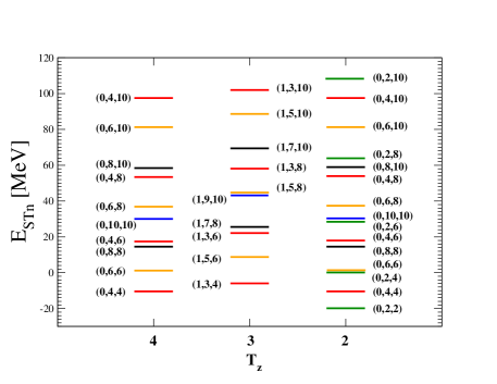
Figure 1: (Color online) Eigenenergies $E_{STn}$ of the Hamiltonian (13) for set of parameters (III), $T_{z}$=4, 3, and 2 and by assuming $H_{I}=0$. Energy states are labeled by spin, isospin, and the SU(4) quantum number $n$: ($S,T,n$). The levels with different value of $S+T$ are displayed in different colors online: $S+T=2$ (green), 4 (red), 6 (orange), 8 (black), and 10 (blue).

In Fig. 1 we present states with energy $E_{STn}$ of different isotopes. The considered level scheme illustrates the situation with double GT transition for ⁴⁸Ca as the isospin and its projection of the initial and final ground states correspond to those of ⁴⁸Ca and ⁴⁸Ti. We note that in nuclear physics the isospin symmetry is conserved to a great extent. Within the studied model in the SU(4) symmetry limit the ground states of ⁴⁸Ca and ⁴⁸Ti can be identified with $S=0$, $T=4$, $T_{z}=4$, $n=4$, and $S=0$, $T=2$, $T_{z}=2$, $n=2$, respectively, and the intermediate states in ⁴⁸Sc with S=1 (T=3,5,7, and 9) T_z=3 (n=4, 6, 8 and 10). As the GT operator is not changing quantum number $n$, the double GT matrix elements connecting initial and final ground states is nonzero only to the extent the breaking of SU(4) symmetry mixes the high-lying (0,4,4) analog of the ⁴⁸Ca ground state into (0,2,2) analog of the ⁴⁸Ti.

IV Double Fermi and GT matrix elements within the perturbation theory

We study the double GT and Fermi matrix elements using perturbation theory within the discussed model close to a point of restoration of the SU(4) symmetry of particle-particle interaction of $H$. First, we assume a conservation of the isospin symmetry by the particle-particle interaction and a subject of interest will be $M^{2\nu}_{GT}$ as function of the isospin of the initial state. Then a weak violation of the isospin symmetry is allowed and the dependence of $M^{2\nu}_{F}$ and $M^{2\nu}_{GT}$ on both quantities $g_{pair}-g_{pp}^{T=0}$ and $g_{pair}-g_{pp}^{T=1}$, which violates the SU(4) symmetry, is analyzed.

IV.1 The GT matrix element in the case of isospin symmetry

We consider a small violation of the SU(4) spin-isospin symmetry in nuclear Hamiltonian (13) due to $g_{pair}\neq g_{pp}^{T=0}$ and that isospin is a good quantum number, i.e., $g_{pair}=g_{pp}^{T=1}$, which implies $M^{2\nu}_{F}=0.$

As an example we discuss in details the GT matrix element for $2\nu\beta\beta$ decay from the state with $S=0$, $T=M_{T}=4$ to the state with $S=0$, $T=M_{T}=2$. The corresponding transition is

$$\ket{0,0,4,4,4}\rightarrow\ket{1,M_{S},3,3,4}\rightarrow\ket{0,0,2,2,2}.$$ (17)

In the case $g_{pair}=g_{pp}^{T=0}$ one finds that $M^{2\nu}_{GT}=0$ as eigenstates of the GT operators are diagonal in SU(4) quantum number $n$ and the initial and final states are assigned into different SU(4) multiplets. By breaking the SU(4) symmetry of particle-particle interaction the quantum number $n$ is not more a good quantum number and states with different $n$ are mixed. By keeping in mind a small violation of this symmetry we denote perturbated states and their energies with a superscript prime symbol ($|S,M_{S},T,M_{T},n^{\prime}\rangle$, $E^{\prime}_{S,M_{S},T,M_{T},n}$), unlike the states with a definite quantum number $n$ ($|S,M_{S},T,M_{T},n\rangle$, $E_{S,M_{S},T,M_{T},n}$).

Up to the second order of parameter $(g_{pair}-g_{pp}^{T=0})$ we get (for sake of simplicity a shorter notation of states and energies (14) is used)

$$E^{\prime}_{022} = E_{022}+\bra{022}H_{I}\ket{022}+\frac{|\bra{024}H_{I}\ket{022}|^{2}}{E_{022}-E_{024}}$$

$$= 12e_{n}+8e_{p}-94g_{pair}+6g_{ph}$$

$$+ (g_{pair}-g_{pp}^{T=0})\frac{132}{5}-\frac{(g_{pair}-g_{pp}^{T=0})^{2}}{10g_{pair}+20g_{ph}}\frac{8316}{25}$$

$$E^{\prime}_{134} = E_{134}+\bra{134}H_{I}\ket{134}+\frac{|\bra{136}H_{I}\ket{134}|^{2}}{E_{134}-E_{136}}$$

$$= 13e_{n}+7e_{p}-84g_{pair}+18g_{ph}$$

$$+ (g_{pair}-g_{pp}^{T=0})\frac{201}{7}-\frac{(g_{pair}-g_{pp}^{T=0})^{2}}{14g_{pair}+28g_{ph}}\frac{10125}{49}$$

$$E^{\prime}_{044} = E_{044}+\bra{044}H_{I}\ket{044}+\frac{|\bra{046}H_{I}\ket{044}|^{2}}{E_{044}-E_{046}}$$

$$= 14e_{n}+6e_{p}-84g_{pair}+12g_{ph}$$

$$+ (g_{pair}-g_{pp}^{T=0})\frac{108}{7}-\frac{(g_{pair}-g_{pp}^{T=0})^{2}}{14g_{pair}+28g_{ph}}\frac{7425}{49}.$$

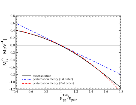
Figure 2: (Color online) Matrix element $M^{2\nu}_{GT}$ for the double-GT two-neutrino double-$\beta$ decay mode as function of ratio $g_{pp}^{T=0}/g_{pair}$ for a set of parameters (III). Exact results are indicated with a solid line. The results obtained within the perturbation theory up to the first and second order in $H_{I}$ contribution to Hamiltonian (13) are shown with dashed-dotted and dashed lines, respectively. The restoration of spin-isospin symmetry of particle-particle interaction is achieved for $g_{pp}^{T=0}/g_{pair}=1$.

For the double GT matrix element we have

$$M^{2\nu}_{GT} = \sum_{n^{\prime}}\frac{\bra{022^{\prime}}\vec{\sigma}\tau^{-}\ket{13n^{\prime}}\cdot\bra{13n^{\prime}}\vec{\sigma}\tau^{-}\ket{044^{\prime}}}{E^{\prime}_{13n}-\left(E^{\prime}_{044}-E^{\prime}_{022}\right)/2},$$ (21)

$$\simeq \frac{\bra{022^{\prime}}\vec{\sigma}\tau^{-}\ket{134^{\prime}}\cdot\bra{134^{\prime}}\vec{\sigma}\tau^{-}\ket{044^{\prime}}}{E^{\prime}_{134}-\left(E^{\prime}_{044}-E^{\prime}_{022}\right)/2}.$$

The allowed intermediate states $\ket{13n^{\prime}}$ are those with $S=1$, $T=3$ and $n^{\prime}=4,6,8$ and $10$. We note that up to second order of perturbation theory there is only a single contribution through the intermediate state $\ket{134^{\prime}}$ and the product of two corresponding $\beta$-amplitudes (numerator of (21) takes the form

$$\left\langle 022^{\prime}\left|\vec{\sigma}\tau^{-}\right|134^{\prime}\right\rangle\cdot\left\langle 134^{\prime}\left|\vec{\sigma}\tau^{-}\right|044^{\prime}\right\rangle=144\sqrt{\frac{231}{35}}$$

$$\times\left(\frac{(g_{pair}-g_{pp}^{T=0})}{10g_{pair}+20g_{ph}}-\frac{267(g_{pair}-g_{pp}^{T=0})^{2}}{35(10g_{pair}+20g_{ph})^{2}}\right).$$

We see that if $g_{pair}=g_{pp}^{T=0}$ GT matrix element vanishes. With help of Eqs. (IV.1), (IV.1) and (IV.1) for the energy denominator in (21) we obtain

$$(2E^{\prime}_{134}-E^{\prime}_{022}-E^{\prime}_{044})/2=5g_{pair}+9g_{ph}$$

$$+(g_{pair}-g_{pp}^{T=0})\frac{39}{5}+\frac{(g_{pair}-g_{pp}^{T=0})^{2}}{g_{pair}+2g_{ph}}\left(\frac{1249263}{171500}\right).$$

It is worth noting that neither the numerator nor denominator of $M^{2\nu}_{GT}$ depend explicitly on the single-particle energies $e_{n}$ and $e_{p}$. If we restrict our consideration to the first-order perturbation theory we find

$$M^{2\nu}_{GT} = \frac{144\sqrt{\frac{231}{35}}(g_{pair}-g_{pp}^{T=0})}{(5g_{pair}+9g_{ph})(10g_{pair}+20g_{ph})}.$$ (24)

In Fig. 2 $M^{2\nu}_{GT}$ is plotted as function of ratio $g_{pp}^{T=0}/g_{pair}$. We see that results obtained within the second-order perturbation theory agree well with exact results within a large range of this parameter. For $g_{pp}^{T=0}/g_{pair}=1$ the restoration of the SU(4) symmetry of particle-particle interaction is achieved, i.e., $M^{2\nu}_{GT}$ is equal to zero. We notice that if the quantity $g_{pp}^{T=0}/g_{pair}$ is within the range (0.8,1.2) the first-order perturbation theory seems to be sufficient.

Usually, ground states of stable even-even nuclei are identified with isospin $T=T_{z}$. The dependence of $M^{2\nu}_{GT}$ on the isospin of the initial nucleus is presented in Fig. 3. We see that for a fixed value of $g_{pp}^{T=0}/g_{pair}$ (i.e., breaking of the SU(4) symmetry) the absolute value of $M^{2\nu}_{GT}$ decreases with increasing isospin $T$. We note that apart from the shell effects of magic nuclei this tendency is observed also for measured $2\nu\beta\beta$-decay matrix elements barabash .

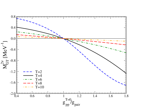
Figure 3: (Color online) Matrix element $M^{2\nu}_{GT}$ for the double-GT two-neutrino double-$\beta$ decay mode as function of ratio $g_{pp}^{T=0}/g_{pair}$ for different initial state with $T=M_{T}$ ($M_{T}=2$, 4, 6, 8, and 10).

IV.2 The Fermi and GT matrix elements in the case of broken SU(2) and SU(4) symmetries

The main task to be addressed in this subsection is determining the dependence of $M^{2\nu}_{F}$ and $M^{2\nu}_{GT}$ on both quantities $g_{pp}^{T=1}/g_{pair}$ and $g_{pp}^{T=0}/g_{pair}$. Recall that $g_{pp}^{T=1}\neq g_{pair}$ breaks both the SU(2) isospin and the SU(4) spin-isospin symmetries of particle-particle interaction unlike $g_{pp}^{T=0}\neq g_{pair}$, which is associated only with the violation of the SU(4) symmetry.

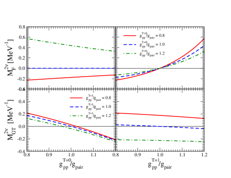
Figure 4: (Color online) Matrix elements $M^{2\nu}_{F}$ and $M^{2\nu}_{GT}$ as function of ratios $g_{pp}^{T=0}/g_{pair}$ and $g_{pp}^{T=1}/g_{pair}$ for transition from the initial $|04^{\prime}4^{\prime}\rangle$ to final $|02^{\prime}2^{\prime}\rangle$ ground state and a set of parameters (III). The results are obtained within the perturbation theory up to the second order.

We consider the $2\nu\beta\beta$-decay transition from the initial $|04^{\prime}4^{\prime}\rangle$ to final $|02^{\prime}2^{\prime}\rangle$ ground state. Up to the first order in the perturbation theory for double Fermi and GT matrix elements we find

$$M^{2\nu}_{F} = -\frac{48\sqrt{\frac{33}{5}}\left(g_{pair}-g_{pp}^{T=1}\right)}{(5g_{pair}+3g_{ph})(10g_{pair}+6g_{ph})},$$ (25)

$$M^{2\nu}_{GT} = \frac{144\sqrt{\frac{33}{5}}}{5g_{pair}+9g_{ph}}\left\{\frac{(g_{pair}-g_{pp}^{T=0})}{(10g_{pair}+20g_{ph})}\right.$$

$$+\left.\frac{2g_{ph}(g_{pair}-g_{pp}^{T=1})}{(10g_{pair}+20g_{ph})(10g_{pair}+6g_{ph})}\right\}.$$

We see that $M^{2\nu}_{F}$ depends only on strength of the isovector interaction $g_{pp}^{T=1}$ unlike $M^{2\nu}_{GT}$, which depends also on the strength of the isoscalar interaction $g_{pp}^{T=0}$. Due to the violation of the isospin symmetry the final ground state $|02^{\prime}2^{\prime}\rangle$ is mixed with both first $|04^{\prime}4^{\prime}\rangle$ and second $|02^{\prime}4^{\prime}\rangle$ excited states (see Fig. 1), resulting in $g_{pp}^{T=1}$ contribution to $M^{2\nu}_{GT}$.

In Fig. 4 we present behavior of $M^{2\nu}_{F}$ and $M^{2\nu}_{GT}$ as function of $g_{pp}^{T=1}/g_{pair}$ ($g_{pp}^{T=0}/g_{pair}$) for a particular values of $g_{pp}^{T=0}/g_{pair}$ ($g_{pp}^{T=1}/g_{pair}$). Results were obtained within the perturbation theory up to the second order. We see clearly that for $g_{pp}^{T=1}/g_{pair}=0$ matrix element $M^{2\nu}_{F}$ does not depend on $g_{pp}^{T=0}$ and varies strongly with change of $g_{pp}^{T=1}$. A different behavior offers $M^{2\nu}_{GT}$, which weakly depends on the $g_{pp}^{T=1}$ and significantly on the $g_{pp}^{T=0}$. These conclusions agree qualitatively well with results obtained for two-neutrino double-$\beta$ decay transitions within the proton-neutron QRPA with restoration of the isospin symmetry newpar13 . The advantage of the study which considered the schematic model and in perturbation theory is that explicit dependence of $M^{2\nu}_{F}$ and $M^{2\nu}_{GT}$ on isoscalar and isovector strength of particle-particle interactions can be determined.

V Energy-weighted sum rule of $\Delta Z=2$ nuclei

In Ref. dusan13 the double Fermi and GT sum rules associated with $\Delta Z=2$ nuclei were introduced. We have

$$S^{ew}_{F}(i,f) \equiv \sum_{n}(E_{n}-\frac{E_{i}+E_{f}}{2})\bra{f}T^{-}\ket{n}\bra{n}T^{-}\ket{i}$$ (27)

$$= \frac{1}{2}\bra{f}\left[T^{-},\left[H,T^{-}\right]\right]\ket{i}$$

$$S^{ew}_{GT}(i,f) \equiv \sum_{n}(E_{n}-\frac{E_{i}+E_{f}}{2})\bra{f}\vec{\cal O}_{GT}\ket{n}\cdot\bra{n}\vec{\cal O}_{GT}\ket{i}$$

$$= \sum_{M}(-1)^{M}\frac{1}{2}\bra{f}\left[({\cal O}_{GT})_{-M},\left[H,({\cal O}_{GT})_{M}\right]\right]\ket{i}$$

with

$$\vec{\cal O}_{GT}=\sum_{k=1}^{A}\tau^{-}_{k}\mathbf{\vec{\sigma}_{k}},$$ (29)

where $|i>$ ($|f>$) are $0^{+}$ ground states of the initial (final) even-even nuclei with energy $E_{i}$ ($E_{f}$), and $|1^{+}_{n}>$ ($|0^{+}_{n}>$) are the $1^{+}$ ($0^{+}$) states in the intermediate odd-odd nucleus with energies $E_{n}$.

If there is a dominance of contribution through a single or few states of the intermediate nucleus, energy-weighted sum rules (27) might be exploited to adjust the strengths of the residual interaction of Hamiltonian for nuclear structure calculations. The left-hand side of Eq. (27) might be determined phenomenologically, unlike the right-hand side of Eq. (27), which requires evaluation of the double commutator within a nuclear model and can be expressed in terms of the strengths of residual interaction. Due to a double commutator of nuclear Hamiltonian with charge-changing Fermi and GT operators connecting states with $\Delta Z=2$ the energy-weighted sum rule $S^{ew}_{F,GT}(i,f)$ does not depend explicitly on the mean field part of the nuclear Hamiltonian.

Table 1: The coefficients $a$, $b$, $c$ and $d$ of the expansion of the energy denominator $E^{\prime}_{n}-\frac{E^{\prime}_{i}+E^{\prime}_{f}}{2}$ [see Eq. (34)] associated with the dominant double GT (double Fermi) transition from the initial ground state $|0T=M_{T}n\rangle$ to the final ground state $|0~{}T=M_{T}-2~{}n-2\rangle$ through a single state of the intermediate nucleus $|1M_{T}~{}n\rangle$ ($|0~{}M_{T}~{}n\rangle$). Coefficients are presented for different isospin $T=M_{T}$ of the initial state.

$T=M_{T}$		Transition	Coefficients
			$a$	$b$	$c$	$d$
2		GT	3	5	$-59/15$	$44/5$
		Fermi	3	3	$50/3$	$-59/5$
4		GT	5	9	$-64/35$	$39/5$
4		Fermi	5	3	$401/35$	-192/35
6		GT	7	13	$-71/63$	$340/63$
		Fermi	7	3	$482/63$	$-71/21$
8		GT	9	17	$-80/99$	$103/33$
		Fermi	9	3	$469/99$	$-80/33$
10		GT	11	21	$-7/11$	$12/11$
		Fermi	11	3	$26/11$	$-21/11$

We analyze $S^{ew}_{F,GT}$ for the Hamiltonian (13) and by exploiting the commutation relations of the SO(8) group. For the case $|i\rangle=|044^{\prime}\rangle$, $|f\rangle=|022^{\prime}\rangle$, we get

$$S^{ew}_{GT}(04^{\prime}4^{\prime},02^{\prime}2^{\prime})\equiv\sum_{n}(E^{\prime}_{13n}-\frac{E^{\prime}_{044}+E^{\prime}_{022}}{2})$$

$$~{}~{}~{}~{}~{}~{}~{}~{}~{}~{}~{}~{}~{}~{}~{}~{}~{}~{}~{}\times\bra{02^{\prime}2^{\prime}}\vec{\sigma}\tau^{-}\ket{13^{\prime}n^{\prime}}\cdot\bra{13^{\prime}n^{\prime}}\vec{\sigma}\tau^{-}\ket{04^{\prime}4^{\prime}}$$

$$=6(g_{pp}^{T=0}-g_{pair})\bra{02^{\prime}2^{\prime}}A_{0,1}^{{}^{\dagger}}(0,-1)A_{0,1}(0,1)\ket{04^{\prime}4^{\prime}}$$

$$-g_{ph}\bra{02^{\prime}2^{\prime}}\vec{\sigma}\tau^{-}\cdot\vec{\sigma}\tau^{-}\ket{04^{\prime}4^{\prime}}-3g_{ph}\bra{02^{\prime}2^{\prime}}T^{-}T^{-}\ket{04^{\prime}4^{\prime}}$$

and

$$S^{ew}_{F}(04^{\prime}4^{\prime},02^{\prime}2^{\prime})\equiv\sum_{n}(E^{\prime}_{0,0,4,3,n}-\frac{E^{\prime}_{044}+E^{\prime}_{022}}{2})$$

$$~{}~{}~{}~{}~{}~{}~{}~{}~{}~{}~{}~{}~{}~{}~{}~{}~{}~{}~{}\times\bra{02^{\prime}2^{\prime}}T^{-}\ket{04^{\prime}n^{\prime}}\cdot\bra{04^{\prime}n^{\prime}}T^{-}\ket{04^{\prime}4^{\prime}}$$

$$=2(g_{pair}-g^{T=1}_{pp})\bra{02^{\prime}2^{\prime}}A_{0,1}^{{}^{\dagger}}(0,-1)A_{0,1}(0,1)\ket{04^{\prime}4^{\prime}}.$$

We note that the dominant contribution to $S^{ew}_{GT}(044^{\prime},022^{\prime})$ and $S^{ew}_{F}(044^{\prime},022^{\prime})$ comes from the transition through the single intermediate states $|134^{\prime}\rangle$ and $|044^{\prime}\rangle$, respectively. By exploiting the first-order perturbation theory to evaluation of matrix elements in Eqs. (V) and (V) for a combination of energies of involved states we find

$$E^{\prime}_{134}-\frac{E^{\prime}_{044}+E^{\prime}_{022}}{2}=5g_{pair}+9g_{ph}$$ (32)

$$~{}~{}~{}~{}~{}~{}~{}~{}-\frac{64}{35}(g_{pair}-g^{T=1}_{pp})+\frac{39}{5}(g_{pair}-g^{T=0}_{pp})$$

$$E^{\prime}_{0,0,4,3,4}-\frac{E^{\prime}_{044}+E^{\prime}_{022}}{2}=5g_{pair}+3g_{ph}$$ (33)

$$~{}~{}~{}~{}~{}+\frac{401}{35}(g_{pair}-g^{T=1}_{pp})-\frac{192}{35}(g_{pair}-g^{T=0}_{pp}).$$

The result in Eq. (V) is in agreement with above calculated expression for energy denominator in Eq. (IV.1), which was derived by assumption of the isospin conservation.

We see that considered energy-weighted sum rules imply useful relations between three energies of states appearing in the denominator of the double GT or Fermi matrix elements and nucleon-nucleon interactions. The energy denominator associated with the dominant double-GT (double-Fermi) transition from the initial ground state $|0T=M_{T}n\rangle$ to the final ground state $|0~{}T=M_{T}-2~{}n-2\rangle$ through a single state of the intermediate nucleus $|1M_{T}~{}n\rangle$ ($|0~{}M_{T}~{}n\rangle$) can be written as

$$E^{\prime}_{n}-\frac{E^{\prime}_{i}+E^{\prime}_{f}}{2}=$$ (34)

$$=ag_{pair}+bg_{ph}+c\left(g_{pair}-g_{pp}^{T=1}\right)+d\left(g_{pair}-g_{pp}^{T=0}\right).$$

Here, $a$, $b$, $c$ and $d$ are coefficients. The perturbation theory up to the first order is considered. For different isospin $T=M_{T}$ of the initial ground-state coefficients $a$, $b$, $c$ and $d$ are presented in Table 1. We see that for larger value of $T$ the value of the energy denominator is affected less by the violation of both the isospin and spin-isospin symmetries as it is for smaller value of $T$.

VI Conclusions

The anatomy of the two-neutrino double-$\beta$ decay matrix elements was studied within a schematic model, which can be solved exactly and yet contains most of the qualitative features of a more realistic description, and by taking advantage of the perturbation theory. We paid attention to violation of both spin-isospin SU(4) and isospin SU(2) symmetries of particle-particle interaction of Hamiltonian. The isospin violation originates from the difference of the proton-proton and the neutron-neutron pairing force compared to the proton-neutron isovector pairing force. The break down of the SU(4) symmetry is a consequence of the difference of the like-nucleon pairing interaction compared to the proton-neutron isoscalar interaction and/or to the proton-neutron isovector interaction, which violates also the isospin symmetry.

By using perturbation theory, an explicit dependence of the two-neutrino double-$\beta$ decay matrix elements on different constituents of the Hamiltonian was established. It was found that the mean-field part of the Hamiltonian does not enter explicitly in the decomposition of $M^{2\nu}_{F}$ and $M^{2\nu}_{GT}$ and is related only to the calculation of unperturbated states of the Hamiltonian. This general conclusion is valid for any mean field approximation. In the case of medium and heavy heavy nuclei the SU(4) symmetry is strongly broken by the spin-orbit splitting, affecting strongly the mean field part, unlike the interaction part of nuclear Hamiltonian. This fact might be an explanation for a smallness of $M^{2\nu}_{GT}$ being governed by a small violation of the SU(4) symmetry by the particle-particle interaction of the Hamiltonian.

The obtained expressions for $M^{2\nu}_{F}$ and $M^{2\nu}_{GT}$ supported by numerical calculation up to the second order in perturbation theory confirm the finding achieved within the proton-neutron QRPA approach that $M^{2\nu}_{F}$ depends strongly on the isovector part of the particle-particle neutron-proton interaction, unlike $M^{2\nu}_{GT}$, which depends strongly on its isoscalar part. By assuming a fixed violation of the SU(4) symmetry by the particle-particle interaction it is shown that value of $M^{2\nu}_{GT}$ decreases by an increase of the isospin of the initial ground state. This tendency is found also in the case of measured double-GT matrix elements being partially spoiled by different pairing properties. We also showed that $M^{2\nu}_{GT}$ contains a small component due to violation of the isospin symmetry. By keeping in mind that in nuclear physics the isospin symmetry is conserved to a great extent it is recommended for evaluation of double-$\beta$ decay matrix elements to use many-body approaches with a conservation or restoration of the isospin symmetry newpar13 ; iachello15 .

An important result coming from the analysis within perturbation theory is that there is a dominance of double-$\beta$ decay transition through a single intermediate state. Further, the importance of the energy-weighted sum rule associated with $\Delta Z=2$ nuclei for fitting different components of the residual interaction of the Hamiltonian was pointed out. It goes without saying that further studies, in particular those in which a realistic nuclear Hamiltonian is used, are of great interest.

Appendix A Operators in SO(8) schematic model

We consider a set of single-particle states with the associated creation and annihilation operators, $a^{\dagger}_{lmm_{s}m_{t}}$ and $a_{lmm_{s}m_{t}}$, which are labeled by orbital angular momentum $l$, its projection on $z$ axis $m$, and $z$ components of spin ($m_{s}=1/2$) and isospin ($m_{t}=1/2$).

The particle-particle operators entering the Hamiltonian (13) are given by pang

$$A_{S,T}^{\dagger}(M_{S},M_{T})=\sum_{l,m,m_{s},m_{t}}\sqrt{l+\frac{1}{2}}C_{lmlm^{\prime}}^{00}C_{\frac{1}{2}m_{t}\frac{1}{2}m_{t}^{\prime}}^{TM_{T}}C_{\frac{1}{2}m_{s}\frac{1}{2}m_{s}^{\prime}}^{SM_{S}}a^{\dagger}_{lmm_{s}m_{t}}a^{\dagger}_{lm^{\prime}m^{\prime}_{s}m^{\prime}_{t}},\quad(S,T)=(0,1)~{}\textrm{or}~{}(1,0),$$ (35)

the particle-hole GT operators take the form

$$E_{a,b}=\sum_{l,m,m_{s},m_{t}}\bra{(m_{s}+a)(m_{t}+b)}\sigma_{a}\tau_{b}\ket{m_{s}m_{t}}a^{\dagger}_{lm(m_{s}+a)(m_{t}+b)}a^{\phantom{\dagger}}_{lmm_{s}m_{t}},$$ (36)

and particle number operators are written as

$$N_{i}=\sum_{l,m,m_{s},m,l}a^{\dagger}_{lmm_{s}{m_{t}}_{i}}a^{\phantom{\dagger}}_{lmm_{s}{{m_{t}}_{i}}},\quad i=p,n,\quad m_{t_{n},t_{p}}=\pm 1/2.$$ (37)

Here, $\sigma_{a}$ and $\tau_{b}$ represent spherical components of the single-particle Pauli spin and isospin operators with convention used in Ref.pang .

Appendix B Relevant SO(8) matrix elements

The matrix elements of SO(8) operators in the basis of zero-seniority states are given in Refs. pang and hechtpang . Here, we present the SO(8) matrix elements relevant for calculation of the double GT and Fermi matrix elements. We have

$$\bra{S,M_{S},T,M_{T},n}\sum_{M_{S}}A^{\dagger}_{1,0}(M_{S},0)A_{1,0}(M_{S},0)\ket{S,M_{S},T,M_{T},n}$$

$$=\frac{(\Omega+n+\lambda+6)(\Omega-n-\lambda)}{8(n+2)(n+3)}\left[\frac{(S+1)(n+S+T+4)(n+S-T+3)+S(n-S+T+3)(n-S-T+2)}{(2S+1)}\right]$$

$$+\frac{(\Omega-n+\lambda+2)(\Omega+n-\lambda+4)}{8(n+1)(n+2)}\left[\frac{(S+1)(n-S+T+1)(n-S-T)+S(n+S-T+1)(n+S+T+2)}{(2S+1)}\right]$$

$$\bra{S,M_{S},T,M_{T},n}\sum_{M_{T}}A^{\dagger}_{0,1}(0,M_{T})A_{0,1}(0,M_{T})\ket{S,M_{S},T,M_{T},n}$$

$$=\frac{(\Omega+n+\lambda+6)(\Omega-n-\lambda)}{8(n+2)(n+3)}\left[\frac{(T+1)(n+T+S+4)(n+T-S+3)+T(n-T+S+3)(n-T-S+2)}{(2T+1)}\right]$$

$$+\frac{(\Omega-n+\lambda+2)(\Omega+n-\lambda+4)}{8(n+1)(n+2)}\left[\frac{(T+1)(n-T+S+1)(n-T-S)+T(n+T-S+1)(n+T+S+2)}{(2T+1)}\right]$$

$$\bra{S,M_{S},T,M_{T},n+2}\sum_{M_{T}}A^{\dagger}_{0,1}(0,M_{T})A_{0,1}(0,M_{T})\ket{S,M_{S},T,M_{T},n}$$

$$=-\bra{S,M_{S},T,M_{T},n+2}\sum_{M_{S}}A^{\dagger}_{1,0}(M_{S},0)A_{1,0}(M_{S},0)\ket{S,M_{S},T,M_{T},n}$$

$$=\frac{1}{8(n+3)}\sqrt{\frac{(\Omega+n+\lambda+6)(\Omega+n-\lambda+6)(\Omega-n+\lambda)(\Omega-n-\lambda)}{(n+2)(n+4)}}$$

$$\times\sqrt{(n+S+T+4)(n+S-T+3)(n-S+T+3)(n-S-T+2)}$$

$$\bra{S,M_{S},T,M_{T},n}\sum_{a,b}E_{ab}^{\dagger}E_{ab}\ket{S,M_{S},T,M_{T},n}$$

$$=n(n+4)-S(S+1)-T(T+1)$$

$$\bra{S,M_{S},T,M_{T},n}A^{\dagger}_{0,1}(0,0)A_{0,1}(0,0)\ket{S,M_{S},T,M_{T},n}$$

$$=\frac{n(\Omega-n+\lambda+2)(\Omega+n-\lambda+4)}{4(n+2)}$$

$$\times\left[\frac{T(n+S+T+2)(n-S+T+1)}{2n(n+1)(2T+1)}\frac{(T-M_{T})(T+M_{T})}{T(2T-1)}+\frac{(T+1)(n+S-T+1)(n-S-T)}{2n(n+1)(2T+1)}\frac{(T+M_{T}+1)(T-M_{T}+1)}{(T+1)(2T+3)}\right]$$

$$+\frac{(n+4)(\Omega+n+\lambda+6)(\Omega-n-\lambda)}{4(n+2)}$$

$$\times\left[\frac{T(n-S-T+2)(n+S-T+3)}{2(n+3)(n+4)(2T+1)}\frac{(T-M_{T})(T+M_{T})}{T(2T-1)}+\frac{(T+1)(n-S+T+3)(n+S+T+4)}{2(n+3)(n+4)(2T+1)}\frac{(T+M_{T}+1)(T-M_{T}+1)}{(T+1)(2T+3)}\right]$$

$$\bra{S,M_{S},T+2,M_{T},n}A^{\dagger}_{0,1}(0,0)A_{0,1}(0,0)\ket{S,M_{S},TM_{T},n,}$$

$$=\sqrt{\frac{(T+M_{T}+1)(T-M_{T}+1)}{(2T+3)(T+1)}}\sqrt{\frac{(T+M_{T}+2)(T-M_{T}+2)}{(2T+3)(T+2)}}$$

$$\times\left[\frac{n(\Omega-n+\lambda+2)(\Omega+n-\lambda+4)}{4(n+2)}\right.\sqrt{\frac{(T+2)(n+S+T+4)(n-S+T+3)}{2n(n+1)(2T+5)}}\sqrt{\frac{(T+1)(n+S-T+1)(n-S-T)}{2n(n+1)(2T+1)}}$$

$$+\left.\frac{(n+4)(\Omega+n+\lambda+6)(\Omega-n-\lambda)}{4(n+2)}\sqrt{\frac{(T+2)(n-S-T)(n+S-T+1)}{2(n+3)(n+4)(2T+5)}}\sqrt{\frac{(T+1)(n-S+T+3)(n+S+T+4)}{2(n+3)(n+4)(2T+1)}}\right]$$

$$\bra{S,M_{S},T,M_{T},n+2}A^{\dagger}_{0,1}(0,0)A_{0,1}(0,0)\ket{S,M_{S},T,M_{T},n}$$

$$=\sqrt{\frac{(n+2)(\Omega-n+\lambda)(\Omega+n-\lambda+6)}{4(n+4)}}\sqrt{\frac{(n+4)(\Omega+n+\lambda+6)(\Omega-n-\lambda)}{4(n+2)}}$$

$$\times\left[\sqrt{\frac{T(n+S+T+4)(n-S+T+3)}{2(n+2)(n+3)(2T+1)}\frac{T(n-S-T+2)(n+S-T+3)}{2(n+3)(n+4)(2T+1)}}\frac{(T-M_{T})(T+M_{T})}{T(2T-1)}\right.$$

$$+\left.\sqrt{\frac{(T+1)(n+S-T+3)(n-S-T+2)}{2(n+2)(n+3)(2T+1)}\frac{(T+1)(n-S+T+3)(n+S+T+4)}{2(n+3)(n+4)(2T+1)}}\frac{(T+M_{T}+1)(T-M_{T}+1)}{(T+1)(2T+3)}\right].$$

$$\bra{S,M_{S},T+2,M_{T},n+2}A^{\dagger}_{0,1}(0,0)A_{0,1}(0,0)\ket{S,M_{S},T,M_{T},n}$$

$$=\sqrt{\frac{(n+2)(\Omega-n+\lambda)(\Omega+n-\lambda+6)}{4(n+4)}}\sqrt{\frac{(n+4)(\Omega+n+\lambda+6)(\Omega-n-\lambda)}{4(n+2)}}\sqrt{\frac{(T+2)(n+S+T+6)(n-S+T+5)}{2(n+2)(n+3)(2T+5)}}$$

$$\times\sqrt{\frac{(T+1)(n-S+T+3)(n+S+T+4)}{2(n+3)(n+4)(2T+1)}}\sqrt{\frac{(T+M_{T}+1)(T-M_{T}+1)}{(2T+3)(T+1)}}\sqrt{\frac{(T+M_{T}+2)(T-M_{T}+2)}{(2T+3)(T+2)}}$$

$$\bra{0,0,T-2,M_{T}-2,n-2}A^{\dagger}_{0,1}(0,-1)A_{0,1}(0,1)\ket{0,0,T,M_{T},n}$$

$$=-\sqrt{\frac{(n+2)(\Omega+n+\lambda+4)(\Omega-n-\lambda+2)}{4n}}\sqrt{\frac{n(\Omega-n+\lambda+2)(\Omega+n-\lambda+4)}{4(n+2)}}\sqrt{\frac{(T-1)(n-1+T)(n+T)}{2(n+1)(n+2)(2T-3)}}$$

$$\times\sqrt{\frac{T(n+T+2)(n+T+1)}{2n(n+1)(2T+1)}}\sqrt{\frac{(T+M_{T}-2)(T+M_{T}-3)}{(2T-2)(2T-1)}}\sqrt{\frac{(T+M_{T}-1)(T+M_{T})}{(2T-1)2T}}$$

$$\bra{0,0,T-2,M_{T}-2,n}A^{\dagger}_{0,1}(0,-1)A_{0,1}(0,1)\ket{0,0,T,M_{T},n}$$

$$=-\sqrt{\frac{(T+M_{T}-2)(T+M_{T}-3)}{(2T-2)(2T-1)}}\sqrt{\frac{(T+M_{T}-1)(T+M_{T})}{(2T-1)2T}}$$

$$\times\left[\frac{n(\Omega-n+\lambda+2)(\Omega+n-\lambda+4)}{4(n+2)}\right.\sqrt{\frac{T(n+T+2)(n+T+1)}{2n(n+1)(2T+1)}}\sqrt{\frac{(T-1)(n-T+3)(n-T+2)}{2n(n+1)(2T-3)}}$$

$$+\left.\frac{(n+4)(\Omega+n+\lambda+6)(\Omega-n-\lambda)}{4(n+2)}\sqrt{\frac{(T-1)(n+T+1)(n+T+2)}{2(n+3)(n+4)(2T-3)}}\sqrt{\frac{T(n-T+2)(n-T+3)}{2(n+3)(n+4)(2T+1)}}\right]$$

$$\bra{0,0,T,M_{T}-2,n}A^{\dagger}_{0,1}(0,-1)A_{0,1}(0,1)\ket{0,0,T,M_{T},n}$$

$$=\frac{n(\Omega-n+\lambda+2)(\Omega+n-\lambda+4)}{4(n+2)}\left[\frac{T(n+T+2)(n+T+1)}{2n(n+1)(2T+1)}\sqrt{\frac{(T-M_{T}+1)(T-M_{T}+2)}{2T(2T-1)}}\sqrt{\frac{(T+M_{T}-1)(T+M_{T})}{2T(2T-1)}}\right.$$

$$+\left.\frac{(T+1)(n-T+1)(n-T)}{2n(n+1)(2T+1)}\sqrt{\frac{(T+M_{T})(T+M_{T}-1)}{(2T+2)(2T+3)}}\sqrt{\frac{(T-M_{T}+1)(T-M_{T}+2)}{(2T+2)(2T+3)}}\right]$$

$$+\frac{(n+4)(\Omega+n+\lambda+6)(\Omega-n-\lambda)}{4(n+2)}\left[\frac{T(n-T+2)(n-T+3)}{2(n+3)(n+4)(2T+1)}\sqrt{\frac{(T-M_{T}+1)(T-M_{T}+2)}{2T(2T-1)}}\sqrt{\frac{(T+M_{T}-1)(T+M_{T})}{2T(2T-1)}}\right.$$

$$+\left.\frac{(T+1)(n+T+3)(n+T+4)}{2(n+3)(n+4)(2T+1)}\sqrt{\frac{(T+M_{T})(T+M_{T}-1)}{(2T+2)(2T+3)}}\sqrt{\frac{(T-M_{T}+1)(T-M_{T}+2)}{(2T+2)(2T+3)}}\right].$$

For $T_{f}=T-2$ the GT matrix element is

$$\sum_{\tilde{n}^{\prime},M_{S}}\bra{0,0,T-2,T-2,\bar{n}^{\prime}}\vec{\sigma}\tau^{-}\ket{1,M_{S},T-1,T-1,\tilde{n}^{\prime}}\cdot\bra{1,M_{S},T-1,T-1,\tilde{n}^{\prime}}\vec{\sigma}\tau^{-}\ket{0,0,T,T,n^{\prime}}$$

$$\equiv \sum_{n,\bar{n}}2c^{\bar{n}^{\prime}}_{0,0,T-2,T-2,\bar{n}}c^{\tilde{n}^{\prime}}_{1,0,T-1,T-1,\bar{n}}c^{\tilde{n}^{\prime}}_{1,0,T-1,T-1,n}c^{n^{\prime}}_{0,0,T,T,n}$$

$$\times \sqrt{\frac{(T-1)T(\bar{n}-T+2)(n-T+3)(n+T+1)(\bar{n}+T+2)}{(2T-1)(2T+1)}}.$$

Within the perturbation theory the subject of interest is the GT matrix element as follows:

$$\sum_{M_{S}}\bra{0,0,4,2,4}\vec{\sigma}\tau^{-}\ket{1,M_{S},3,3,4}\cdot\bra{1,M_{S},3,3,4}\vec{\sigma}\tau^{-}\ket{0,0,4,4,4}=-\frac{12}{\sqrt{7}}.$$

References

- (1) J.D. Vergados, H. Ejiri, and F. Šimkovic, Rep. Prog. Phys. 75, 106301 (2012).
- (2) E. Caurier, F. Nowacki, and A. Poves, Phys. Lett. B 711, 62 (2012).
- (3) R.A. Sen’kov and M. Horoi, Phys. Rev. C 88, 064312 (2013).
- (4) J. Barea, J. Kotila, and F. Iachello, Phys. Rev. C 87, 014315 (2013).
- (5) P.K. Rath, R. Chandra, K. Chaturvedi, P. Lohani, P. K. Raina, and J. G. Hirsch,, Phys. Rev. C 88 (2013) 064322.
- (6) T.R. Rodriguez and G. Martinez-Pinedo, Phys. Rev. Lett. 105 (2010) 252503.
- (7) F. Šimkovic, A. Faessler, H. Muther, V. Rodin, and M. Stauf, Phys. Rev. C 79, 055501 (2009).
- (8) F. Šimkovic, V. Rodin, A. Faessler, and P. Vogel, Phys. Rev. C 87, 045501 (2013).
- (9) V. Rodin and A. Faessler, Phys. Rev. C 84, 014322 (2011).
- (10) W.C. Haxton and G.J. Stephenson, Jr., Prog. Part. Nucl. Phys. 12, 409 (1984).
- (11) M. Doi, T. Kotani, E. Takasugi, Prog. Theor. Phys. Suppl. 83, 1 (1985).
- (12) A.S. Barabash, Nucl. Phys. A 935, 52 (2015).
- (13) P. Vogel, M. Ericson, and J.D. Vergados, Phys. Lett. B 212, 259 (1988).
- (14) J. Bernabeu, B. Desplanques, J. Navarro, and S. Noguera, Z. Phys. C 46, 323 (1990).
- (15) P. Vogel and M.R. Zirnbauer, Phys. Rev. Lett. 57, 3148 (1986).
- (16) J. Engel, S. Pittel, M. Stoitsov, P. Vogel, and J. Dukelsky, Phys. Rev. C 55, 1781 (1997).
- (17) D. Štefánik, F. Šimkovic, K. Muto, and A. Faessler, Phys. Rev. C 88, 025503 (2013).
- (18) S.C. Pang, Nucl. Phys. A 128,497 (1969).
- (19) K.T.Hecht and S.C.Pang, J. Math. Phys. 10, 1571 (1969).
- (20) B.H. Flowers and S. Szpikowski, Proc. Phys. Soc. 84, 673 (1964).
- (21) J.A. Evans et al., Nucl. Phys. A 367, 77 (1981).
- (22) J. Barea, J. Kotila, F. Iachello, Phys. Rev. C 91, 034304 (2015).