Complexities of 3-manifolds from triangulations, Heegaard splittings, and surgery presentations

Abstract.

We study complexities of 3-manifolds defined from triangulations, Heegaard splittings, and surgery presentations. We show that these complexities are related by linear inequalities, by presenting explicit geometric constructions. We also show that our linear inequalities are asymptotically optimal. Our results are used in [Cha16b] to estimate Cheeger-Gromov $L^{2}$ $\rho$-invariants in terms of geometric group theoretic and knot theoretic data.

1. Introduction and main results

In this paper we study the relationship between various notions of complexities of 3-manifolds. In what follows, we always assume that 3-manifolds are compact.

Simplicial complexity

The first notion of complexity we consider is defined from triangulations. In this paper a triangulation designates a simplicial complex structure.

Definition 1.1.

For a 3-manifold $M$, the simplicial complexity $c^{\text{simp}}(M)$ is defined to be the minimal number of 3-simplices in a triangulation of $M$.

A similar notion of complexity defined from more flexible triangulations is often considered in the literature (e.g., see [MPV09, JRT09, JRT11, JRT13]): a pseudo-simplicial triangulation of a $3$-manifold $M$ is defined to be a collection of $3$-simplices together with affine identifications of faces from which $M$ is obtained as the quotient space. The pseudo-simplicial complexity, or the complexity $c(M)$ of $M$ is defined to be the minimal number of $3$-simplices in a pseudo-simplicial triangulation. For closed irreducible 3-manifolds, $c(M)$ agrees with Matveev’s complexity [Mat90] defined in terms of spines, unless $M=S^{3}$, $\mathbb{R}P^{3}$, or $L(3,1)$. Since the second barycentric subdivision of a pseudo-simplicial triangulation is a triangulation and a 3-simplex is decomposed to $(4!)^{2}=576$ 3-simplices in the second barycentric subdivision, we have

$$\frac{1}{576}\cdot c^{\text{simp}}(M)\leq c(M)\leq c^{\text{simp}}(M).$$

Heegaard-Lickorish complexity

Recall that a Heegaard splitting of a closed 3-manifold is represented by a mapping class in the mapping class group $\operatorname{Mod}(\Sigma_{g})$ of a surface $\Sigma_{g}$ of genus $g$. (Our precise convention is described in the beginning of Section 3. The identity mapping class gives the standard Heegaard splitting of $S^{3}$ shown in Figure 1.) It is well known that $\operatorname{Mod}(\Sigma_{g})$ is finitely generated; Lickorish showed that $\operatorname{Mod}(\Sigma_{g})$ is generated by the $\pm 1$ Dehn twists about the $3g-1$ curves $\alpha_{i}$, $\beta_{i}$, and $\gamma_{i}$ shown in Figure 1 [Lic62, Lic64].

0mm $\alpha_{1}$ at 46 70 $\beta_{1}$ at 34 14 $\gamma_{1}$ at 93 65 $\alpha_{2}$ at 138 70 $\beta_{2}$ at 124 14 $\gamma_{2}$ at 180 65 $\gamma_{g-1}$ at 228 65 $\alpha_{g}$ at 264 70 $\beta_{g}$ at 250 14

$$\Sigma_{g}=\;\vbox{\hbox{\includegraphics[scale={.8}]{lickorish-generators-complexities}}}$$

Figure 1. Standard Dehn twist curves of Lickorish.

From this, a geometric group theoretic notion of complexity is defined for 3-manifolds as follows.

Definition 1.2.

The Heegaard-Lickorish complexity $c^{\text{HL}}(M)$ of a closed $3$-manifold $M$ is defined to be the minimal word length, with respect to the Lickorish generators, of a mapping class $h\in\operatorname{Mod}(\Sigma_{g})$ on a surface $\Sigma_{g}$ of arbitrary genus which gives a Heegaard splitting of $M$.

Note that both the genus $g$ of a Heegard surface $\Sigma_{g}$ and the mapping class $h$ vary in taking the minimum in Definition 1.2. By definition, $c^{\text{HL}}(S^{3})=0$.

We remark that the Heegaard-Lickorish complexity tells us more delicate information than the Heegaard genus. It turns out that the difference of the Heegaard-Lickorish complexities of two $3$-manifolds with the same Heegaard genus can be arbitrarily large, whereas the Heegaard genus of a 3-manifold is bounded by twice its Heegaard-Lickorish complexity. See Lemma 3.1 and related discussions in Section 3.

Our first result is the following relationship between the two complexities defined above.

Theorem A.

For any closed 3-manifold $M\neq S^{3}$, $c^{\text{simp}}(M)\leq 552\cdot c^{\text{HL}}(M)$.

We remark that upper bounds to (pseudo-)simplicial complexity in terms of a Heegaard splitting were studied earlier in the literature, for instance see [Mat90, Proposition 3] and [Mat07, Proposition 2.1.8]. In many cases Theorem A provides a sharper upper bound. For more about this, see Remark 3.5 as well as Theorems C and D below which concern the optimality of our bound. The optimality is essential in an application of [Cha16b] (see the last part of the introduction).

Surgery complexity

To define another notion of complexity of 3-manifolds from knot theoretic information, we consider Dehn surgery with integral coefficients. For a framed link $L$ in $S^{3}$, let $f(L)=\sum_{i}|f_{i}(L)|$ where $f_{i}(L)\in\mathbb{Z}$ is the framing on the $i$th component of $L$. If a component $K$ of $L$ is contained in an embedded 3-ball in $S^{3}$ which is disjoint from other components, then we call $K$ a split component. Let $n(L)$ be the number of split unknotted zero framed components of $L$. An example with $f(L)=2$, $n(L)=1$ is illustrated in Figure 2. We denote by $c(L)$ the crossing number of a link $L$ in $S^{3}$, that is, $c(L)$ is the minimal number of crossings in a planar diagram of $L$. As a convention, if $L$ is empty, then $c(L)=f(L)=n(L)=0$.

Figure 2. A framed link $L$ with $f(L)=2$, $n(L)=1$.

Definition 1.3.

The surgery complexity of a closed 3-manifold $M$ is defined by

$$c^{\text{surg}}(M)=\min_{L}\{2c(L)+f(L)+n(L)\}$$

where $L$ varies over framed links in $S^{3}$ from which $M$ is obtained by surgery.

We remark that we bring in $n(L)$ to detect $S^{1}\times S^{2}$ summands, which can be added to any 3-manifold by connected sum without altering $c(L)$ and $f(L)$ of a framed link $L$ giving the 3-manifold. Note that $n(L)=0$ for any $L$ that gives $M$ if $M$ has no $S^{1}\times S^{2}$ summand. In particular it is the case if $M$ is irreducible. Note that $c^{\text{surg}}(S^{3})=0$ by our convention.

Our second result is the following relationship between the simplicial complexity and the surgery complexity.

Theorem B.

For any closed 3-manifold $M\neq S^{3}$, $c^{\text{simp}}(M)\leq 72\cdot c^{\text{surg}}(M)$.

We remark that Matveev gave a similar inequality which relates the complexity $c(M)$ to a surgery presentation [Mat07, Proposition 2.1.13]

The proofs of Theorems A and B consist of geometric arguments which explicitly construct triangulations from Heegaard splittings and from surgery presentations. Details are given in Sections 2 and 3.

Optimality of Theorems A and B

It is natural to ask how sharp the inequalities in Theorems A and B are. This seems to be a nontrivial problem, since it appears to be hard to determine the complexities we consider, or even to find an efficient lower bound for them. We remark that the determination and lower bound problems for the pseudo-simplicial complexity $c(M)$ have been studied extensively in the literature and regarded as difficult problems [Mat03, JRT13].

We show that the linear inequalities in Theorems A and B are asymptotically optimal. This can be described in terms of standard notations for asymptotic growth, as follows. Recall that we write $f(n)\in O(g(n))$ if $f$ is bounded above by $g$ asymptotically, that is, $\limsup_{n\mathchoice{\longrightarrow}{\rightarrow}{\rightarrow}{\rightarrow}\infty}|f(n)/g(n)|$ is finite. Also, $f(n)\in o(g(n))$ if $f(n)$ is dominated by $g(n)$ asymptotically, that is, $\limsup_{n\mathchoice{\longrightarrow}{\rightarrow}{\rightarrow}{\rightarrow}\infty}|f(n)/g(n)|=0$. We write $f(n)\in\Omega(g(n))$ if $f(n)$ is not dominated by $g(n)$.

Define two functions $s_{\text{HL}}(\ell)$ and $s_{\text{surg}}(k)$ by

$$s_{\text{HL}}(\ell) =\sup\{c^{\text{simp}}(M)\mid c^{\text{HL}}(M)\leq\ell\},$$

$$s_{\text{surg}}(k) =\sup\{c^{\text{simp}}(M)\mid c^{\text{surg}}(M)\leq k\},$$

where the supremums exist by Theorems A and B. In other words, $s_{\text{HL}}(\ell)$ is the “largest possible value” of the simplicial complexity for 3-manifolds with Heegaard-Lickorish complexity $\ell$ or less. We can interpret $s_{\text{surg}}(k)$ similarly.

Theorem C.

$s_{\text{HL}}(\ell)\in O(\ell)\cap\Omega(\ell)$ and $s_{\text{surg}}(k)\in O(k)\cap\Omega(k)$.

As explicit examples, the lens spaces $L(n,1)$ satisfy the following:

Theorem D.

For any $n>3$,

$$\frac{1}{4357080}\cdot c^{\text{HL}}(L(n,1))\leq c^{\text{simp}}(L(n,1)),$$

$$\frac{1}{4357080}\cdot c^{\text{surg}}(L(n,1))\leq c^{\text{simp}}(L(n,1)).$$

We also prove a similar inequality for a larger class of 3-manifolds. See Theorem 4.4 and related discussions in Section 4.

The proofs of Theorems C and D are given in Section 4.

Applications to universal bounds for Cheeger-Gromov invariants

Results in this paper are closely related to the recent development of a topological approach to the universal bounds of Cheeger-Gromov $L^{2}$ $\rho$-invariants in [Cha16b]. In fact, Theorems A and B of this paper are used as essential ingredients in [Cha16b] to give explicit linear estimates of Cheeger-Gromov $\rho$-invariants of 3-manifolds in terms of geometric group theoretical and knot theoretical data. See Theorems 1.8 and 1.9 of [Cha16b]. This application is a major motivation of the present paper. Our inequalities in Theorems A and B are sharp enough, compared with earlier similar work, to give results that the linear estimates in [Cha16b] are asymptotically optimal. See Theorem 7.8 of [Cha16b].

On the other hand, the lower bounds in Theorem D are proven by employing results of [Cha16b] which relate triangulations and the Cheeger-Gromov $\rho$-invariants. See Section 4 for more details.

Acknowledgements

The author thanks an anonymous referee for comments which were very helpful in improving results and in fixing a mistake of an earlier version of this paper. This work was partially supported by NRF grants 2013067043 and 2013053914.

2. Linear complexity triangulations from surgery presentations

In this section we present a construction of a triangulation from a surgery presentation.

Lemma 2.1.

Suppose $L$ is a framed link in $S^{3}$. Suppose there is a planar diagram $D$ with $c$ or fewer crossings for $L$, in which there is no local kink ( , ) and each zero framed component of $L$ is involved in a crossing. Let $w_{i}\in\mathbb{Z}$ be the writhe of the $i$th component in the diagram $D$. Then the 3-manifold $M$ obtained by surgery on $L$ has simplicial complexity at most $96c+48\sum|f_{i}(L)-w_{i}|$.

Example 2.2.

Consider the stevedore knot, which is $6_{1}$ in the table in Rolfsen [Rol76], or KnotInfo [CL]. It has a planar diagram with 6 crossings, where 2 of them have the same sign but the other 4 have the opposite sign. It follows that the zero surgery manifold $M$ of $6_{1}$ satisfies $c^{\text{simp}}(M)\leq 96\cdot 6+48\cdot 2=672$.

Before we prove Lemma 2.1, we prove Theorem B using Lemma 2.1.

Proof of Theorem B.

Recall that Theorem B says

$$c^{\text{simp}}(M)\leq 72\cdot c^{\text{surg}}(M)$$

for $M\neq S^{3}$.

We need the following two observations: firstly, we have

(2.1) $$c^{\text{simp}}(M_{1}\#M_{2})\leq c^{\text{simp}}(M_{1})+c^{\text{simp}}(M_{2})-2,$$

since the connected sum of two triangulated 3-manifolds can be performed by deleting a 3-simplex from each and then glueing faces. Second, we have

(2.2) $$c^{\text{simp}}(S^{1}\times S^{2})\leq 72.$$

For instance, by taking the product of a triangle triangulation of $S^{1}$ and its suspension which is a triangulation of $S^{2}$, and then by applying the standard prism decomposition to each product $\Delta^{1}\times\Delta^{2}$ (see Figure 3), we obtain a triangulation of $S^{1}\times S^{2}$ with $3\cdot 6\cdot 3=54$ tetrahedra.

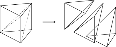
Figure 3. Prism decomposition of $\Delta^{1}\times\Delta^{2}$.

Choose a framed link $L$ such that $M$ is obtained by surgery on $L$ and $2c(L)+f(L)+n(L)=c^{\text{surg}}(M)$. Choose a planar diagram $D$ for $L$ with minimal number of crossings, and let $D_{0}$ be the subdiagram of $D$ consisting of zero framed split components of $L$. From the minimality, it follows that $D$ has no local kink and $D_{0}$ consists of zero framed circles with no crossing. Also every zero framed component of $L$ in $D-D_{0}$ is involved in a crossing. Let $M^{\prime}$ be the 3-manifold obtained by surgery along the given framing of $D-D_{0}$. Since a component of $D_{0}$ contributes an $S^{1}\times S^{2}$ summand, $M=M^{\prime}\mathbin{\#}(n(L)\cdot(S^{1}\times S^{2}))$.

If $D=D_{0}$, then $c(L)=f(L)=0$ and $M^{\prime}=S^{3}$; also, $n(L)\geq 1$ since $M\neq S^{3}$. It follows that

$$c^{\text{simp}}(M)\leq n(L)\cdot c^{\text{simp}}(S^{1}\times S^{2})\leq 72\cdot n(L)$$

by using (2.1) and (2.2). This is the desired conclusion for this case.

If $D\neq D_{0}$, we have

(2.3) $$c^{\text{simp}}(M)\leq c^{\text{simp}}(M^{\prime})+n(L)\cdot c^{\text{simp}}(S^{1}\times S^{2})\leq c^{\text{simp}}(M^{\prime})+72\cdot n(L)$$

by using (2.1) and (2.2). The number of crossings of $D-D_{0}$ is equal to that of $D$, which is equal to $c(L)$ by our choice of $D$. Let $w_{i}$ be the writhe of the $i$th component in $D-D_{0}$, and $f_{i}$ be its given framing. Since a crossing in the diagram contributes $1$, $0$, or $-1$ to $w_{i}$ for some $i$, it follows that $\sum|w_{i}|\leq c(L)$. Therefore we have

(2.4) $$c^{\text{simp}}(M^{\prime}) \leq 96\cdot c(L)+48\cdot\sum|f_{i}-w_{i}|$$

$$\leq 96\cdot c(L)+48\cdot(f(L)+c(L))\leq 72\cdot(2c(L)+f(L))$$

by Lemma 2.1. From (2.3) and (2.4), the desired conclusion follows. ∎

Proof of Lemma 2.1.

We will construct a triangulation of the exterior of $L$ which is motivated from J. Weeks’ SnapPea (see [Wee05]), and then will triangulate the Dehn filling tori in a compatible way.

In what follows we view $D$ as a planar diagram lying on $S^{2}$. By the subadditivity (2.1), we may assume that the diagram $D$ is nonsplit, that is, any simple closed curve in $S^{2}$ disjoint from $D$ bounds a disk disjoint from $D$. This is equivalent to that every region of $D$ is a disk.

Either $D$ has at least one crossing, or $D$ is a circle with no crossings. First, suppose that it is the former case.

Consider the dual graph $G_{0}$ of $D$, whose regions are quadrangles corresponding to crossings. (Since $D$ has no local kinks, the four vertices of each quadrangles are mutually distinct.) For each component of the link $L$, choose an edge of $G_{0}$ which is dual to the component (that is, the edge intersects a strand of $D$ that belongs to the component), and add $2|f_{i}-w_{i}|$ parallels of the edge, where $f_{i}=f_{i}(L)$ is the framing and $w_{i}\in\mathbb{Z}$ is the writhe of the component. Denote the resulting graph by $G$. For an example, see the left of Figure 4, which illustrates the case of a $(+1)$-framed figure eight.

View the link $L$ as a submanifold of $S^{2}\times[-1,1]$ which projects to $D$ under $S^{2}\times[-1,1]\mathchoice{\longrightarrow}{\rightarrow}{\rightarrow}{\rightarrow}S^{2}$, and remove from $S^{2}\times[-1,1]$ an open tubular neighborhood $\nu(L)$ of $L$ which is tangential to $S^{2}\times\{-1,1\}$ at $(\text{each crossing})\times\{-1,1\}$; cutting along $G\times[-1,1]$, we obtain pieces of two types: (i) cubes with two tunnels, which correspond to the crossings of $D$, and (ii) those of the form $(\text{2-gon})\times[-1,1]$ with a tunnel removed, which correspond to the edges of $G-G_{0}$. See the middle of Figure 4.

$D$ at 85 235 $G$ at 20 136 type (i) at 240 140 type (ii) at 240 20

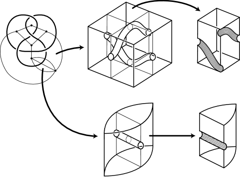
Figure 4. A decomposition of a link diagram.

Cut each piece along $D\times[-1,1]$. In case of type (i), we obtain 4 equivalent subpieces. See the top right of Figure 4. The hatched quadrangles represent $\partial\nu(L)$. Each of the 4 subpieces can be viewed as a cube shown in the left of Figure 5. Let $p$ be the vertex shown in Figure 5, and triangulate the three square faces not adjacent to $p$ as in the left of Figure 5. By taking a cone from $p$, we obtain a triangulation of the each type (i) subpiece. Since the triangulation of the faces away from $p$ has 14 triangles, the cone triangulation of a type (i) subpiece has 14 tetrahedra.

$p$ at 49 55 $q$ at 237 68

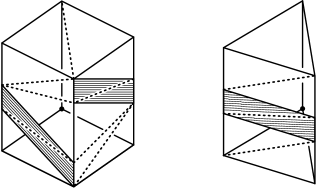
Figure 5. Decomposition of subpieces.

In case of type (ii), by cutting each piece along $D\times[-1,1]$, we obtain two subpieces each of which are as in the bottom right of Figure 4. For each type (ii) subpiece, triangulate the front face as shown in the right of Figure 5, and then triangulate the subpiece by taking the cone of the union of the front face and top triangle from the vertex $q$, similarly to the above type (i) case. This triangulation of a type (ii) subpiece has 7 tetrahedra.

Suppose $D$ has $c$ crossings. For brevity, denote $\delta:=\sum|f_{i}-w_{i}|$. There are $4c$ subpieces of type (i) and $4\delta$ subpieces of type (ii). By applying the above to each of them, we obtain a triangulation of $S^{2}\times[-1,1]\smallsetminus\nu(L)$, which has $14\cdot 4c+7\cdot 4\delta=56c+28\delta$ tetrahedra.

For $t=\pm 1$, the triangulation restricts to a triangulation of $S^{2}\times\{t\}$ with $8c+4\delta$ triangles, since the top of type (i) and (ii) subpieces consist of two triangles and a single triangle respectively. Attaching two $3$-balls triangulated as the cone of these triangulations, we obtain a triangulation of $S^{3}\smallsetminus\nu(L)$ which has $(56c+28\delta)+2\cdot(8c+4\delta)=72c+36\delta$ tetrahedra.

In our triangulation, there are $8c+4\delta$ hatched quadrangular regions, and they are paired up to form $4c+2\delta$ annuli, and the $i$th boundary component of $\nu(L)$ is a union of $2k_{i}+2|f_{i}-w_{i}|$ such annuli, where $k_{i}$ is the number of times the $i$th component of $L$ passes through a crossing. We have $\sum k_{i}=2c$. (Since a component may pass through the same crossing twice, $k_{i}$ may not be equal to the number of crossings that the component passes through.) See the left of Figure 6; the hatched meridional annulus is one of these $2k_{i}+2|f_{i}-w_{i}|$ annuli.

$\alpha_{i}$ at 33 107 $\alpha^{\prime}_{i}$ at 17 74 from type (i) (untwisted) at 60 50 from type (ii) (twisted) at 105 50 from type (i) (untwisted) at 150 50 the $i$th component of $\partial\nu(L)$ at 193 68 $\alpha_{i}$ at 296 74 $\alpha^{\prime}_{i}$ at 295 156 $D^{2}\times S^{1}$ at 255 66 $\alpha_{i}$ at 267 8 $\alpha^{\prime}_{i}$ at 365 8

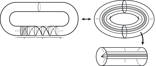
Figure 6. A boundary component and a Dehn filling torus.

On the $i$th boundary component of $\nu(L)$, take the top and bottom edges of the hatched quadrangles in type (i) subpieces, and the diagonal edges used to triangulate the hatched quadrangles in type (ii) subpieces. We may assume that the union of these edges consists of two parallel circles, say $\alpha_{i}$ and $\alpha^{\prime}_{i}$, by appropriately altering the choices of diagonals used above to triangulate the hatched quadrangles if necessary. See the left of Figure 6 in which $\alpha_{i}$ and $\alpha^{\prime}_{i}$ are shown as thick curves. Moreover we may assume that the framing represented by $\alpha_{i}$ differs from the blackboard framing by $f_{i}-w_{i}$; that is, whenever $\alpha_{i}$ passes through a type (ii) piece, a half twist with the same sign as that of $f_{i}-w_{i}$ is introduced with respect to the blackboard framing, while $\alpha_{i}$ runs along the blackboard framing in type (i) pieces. See the left of Figure 6, which illustrates the case of $f_{i}-w_{i}=1$. Since the blackboard framing is equal to $w_{i}$, it follows that $\alpha_{i}$ represents the given framing $f_{i}$.

Take a solid torus $D^{2}\times S^{1}$ for each component of $L$. Attach the solid tori to the exterior $S^{3}\smallsetminus\nu(L)$ along orientation reversing homeomorphisms of boundary tori which takes the curves $\alpha_{i}$ and $\alpha^{\prime}_{i}$ to meridians bounding disks and takes a hatched annulus to a longitudinal annulus, as shown in Figure 6. Pulling back the triangulation of $\partial(S^{3}\smallsetminus\nu(L))$, we obtain a triangulation of $\partial(D^{2}\times S^{1}$). It extends to a triangulation of $D^{2}\times S^{1}$ as follows. By cutting the $D^{2}\times S^{1}$ along the meridional disks bounded by $\alpha_{i}$ and $\alpha^{\prime}_{i}$, we obtain two solid cylinders $D^{2}\times[0,1]$. Note that we already have $2k_{i}+2|f_{i}-w_{i}|$ vertices on $\partial D^{2}\times 0$. We triangulate $D^{2}\times 0$ into $2k_{i}+2|f_{i}-w_{i}|$ triangles, by drawing edges joining the vertices to the center of $D^{2}\times 0$. See the bottom of Figure 6. Taking the product with $[0,1]$, we decompose $D^{2}\times[0,1]$ into $2k_{i}+2|f_{i}-w_{i}|$ triangular prisms. Note that each prism corresponds to a hatched quadrangle. Finally we apply the standard prism decomposition (Figure 3) to each prism. Since each prism gives 3 tetrahedra and there are $8c+4\delta$ hatched quadrangles, the union of all the Dehn filling solid tori is decomposed into $3(8c+4\delta)=24c+12\delta$ tetrahedra.

The triangulation of our surgery manifold $M$ is obtained by adjoining the Dehn filling tori triangulations to that of the exterior. By the above tetrahedra counting, it follows that the number of tetrahedra in $M$ is at most $(72c+36\delta)+(24c+12\delta)=96c+48\delta$. This completes the proof when there is at least one crossing in $D$.

Now, suppose $D$ consists of a single circle without crossings. Note that the writhe is zero in this case. Let $f_{1}\in\mathbb{Z}$ be the given framing. By the hypothesis, $f_{1}\neq 0$. We need to prove that $c^{\text{simp}}(M)\leq 48|f_{1}|$. If $f_{1}=\pm 1$, then $M=L(f_{1},1)=S^{3}$, and it is straightforward to verify that $c^{\text{simp}}(S^{3})\leq 48$. (For instance, triangulate the equator $S^{2}\subset S^{3}$ into 4 triangles, by viewing it as the boundary of a 3-simplex, and triangulate the upper and lower hemispheres by taking a cone of the equator, to obtain a triangulation of $S^{3}$ with $8$ tetrahedra.) Suppose $|f_{1}|\geq 2$. Note that the dual graph $G_{0}$ of $D$ consists of two vertices and a single edge joining them. Let $G$ be the graph obtained by adding $2|f_{1}|-1$ parallels of the edge, that is, $G$ consists of $2|f_{1}|$ edges between the two vertices. Apply the same construction as above, using this $G$, to triangulate $M$. In this case we have $2|f_{1}|$ type (ii) pieces and no type (i) pieces. Using $|f_{1}|\geq 2$, it is verified that our construction produces a simplicial complex structure. (No two vertices of a tetrahedron are identified and each tetrahedron is uniquely determined by its vertices.) By the above counting, the number of tetrahedra is $48|f_{1}|$, as desired. ∎

3. Linear complexity triangulations from Heegaard splittings

In this section we present an explicit construction of a triangulation from a Heegaard splitting given by a mapping class. Recall from Definition 1.2 that the Heegaard-Lickorish complexity of a closed $3$-manifold $M$ is the minimal word length, in the Lickorish generators, of a mapping class on an arbitrary surface which gives a Heegaard splitting of $M$. Here the Lickorish generators of the mapping class group $\operatorname{Mod}(\Sigma_{g})$ of an oriented surface $\Sigma_{g}$ of genus $g$ are defined to be the $\pm 1$ Dehn twists along the curves $\alpha_{1},\ldots,\alpha_{g}$, $\beta_{1},\ldots,\beta_{g}$, $\gamma_{1},\ldots,\gamma_{g-1}$ shown in Figure 1.

To make it precise, we use the following convention. Fix a standard embedding of a surface $\Sigma_{g}$ of genus $g$ in $S^{3}$ as in Figure 1. Then $\Sigma_{g}$ bounds the inner handlebody $H_{1}$ and the outer handlebody $H_{2}$ in $S^{3}$. Let $i_{j}\colon\Sigma_{g}\mathchoice{\longrightarrow}{\rightarrow}{\rightarrow}{\rightarrow}H_{j}$ ($j=1,2$) be the inclusion. The mapping class $h\in\operatorname{Mod}(\Sigma_{g})$ of a homeomorphism $f\colon\Sigma_{g}\mathchoice{\longrightarrow}{\rightarrow}{\rightarrow}{\rightarrow}\Sigma_{g}$ gives a Heegaard splitting $(\Sigma_{g},\{\beta_{i}\},\{f(\alpha_{i})\})$ of the $3$-manifold

$$M=(H_{1}\cup H_{2})/i_{1}(f(x))\sim i_{2}(x),\ x\in\Sigma_{g}.$$

In other words, $M$ is obtained by attaching $g$ $2$-handles to the inner handlebody $H_{1}$ with boundary $\Sigma_{g}$ along the curves $f(\alpha_{i})$ and then attaching a $3$-handle. Under our convention, the identity mapping class gives us $S^{3}$.

The Heegaard-Lickorish complexity can be compared with the Heegaard genus by the following lemma.

Lemma 3.1.

Suppose $M$ is a closed $3$-manifold with a Heegaard splitting given by a mapping class $h\in\operatorname{Mod}(\Sigma_{g})$ which is a product of $\ell$ Lickorish generators. Then for some $g^{\prime}\leq 2\ell$, $M$ admits a Heegaard splitting given by a mapping class $h^{\prime}\in\operatorname{Mod}(\Sigma_{g^{\prime}})$ which is a product of $\ell$ Lickorish generators.

From Lemma 3.1, it follows immediately that the Heegaard genus is not greater than twice the Heegaard-Lickorish complexity. On the other hand, it is easily seen that a 3-manifold may be drastically more complicated than another with the same Heegaard genus. For example, all the lens spaces $L(n,1)$ have Heegaard genus one, but $L(n,1)$ is represented by a genus one mapping class of Heegaard-Lickorish word length $n$. In fact, by results of [Cha16b] (see also Lemma 4.2 and related discussions in the present paper), $c^{\text{simp}}(L(n,1))\mathchoice{\longrightarrow}{\rightarrow}{\rightarrow}{\rightarrow}\infty$ as $n\mathchoice{\longrightarrow}{\rightarrow}{\rightarrow}{\rightarrow}\infty$, and consequently $c^{\text{HL}}(L(n,1))\mathchoice{\longrightarrow}{\rightarrow}{\rightarrow}{\rightarrow}\infty$ and $c^{\text{surg}}(L(n,1))\mathchoice{\longrightarrow}{\rightarrow}{\rightarrow}{\rightarrow}\infty$ by Theorems A and B.

Proof of Lemma 3.1.

For a Lickorish generator $t\in\operatorname{Mod}(\Sigma_{g})$, we say that $t$ passes through the $i$th hole of $\Sigma_{g}$ if $t$ is a Dehn twist along either one of the curves $\alpha_{i}$, $\beta_{i}$, $\gamma_{i}$ or $\gamma_{i-1}$ (see Figure 1). It is easily seen from Figure 1 that a Lickorish generator can pass through at most two holes of $\Sigma_{g}$. Therefore, the Lickorish generators which appear in the given word expression of $h$ of length $\ell$ can pass through at most $2\ell$ holes. If $g>2\ell$, then for some $i$, no Lickorish generator used in $h$ passes through the $i$th hole. By a destabilization which removes the $i$th hole from $\Sigma_{g}$, we obtain a Heegaard splitting of $M$ of genus $g-1$ given by a mapping class which is a product of $\ell$ Lickorish generators. By an induction, the proof is completed. ∎

Lickorish’s work [Lic62, Lic64] presents a construction of a surgery presentation from a Heegaard splitting. From his proof, we obtain the following:

Theorem 3.2.

For any closed 3-manifold $M$, $c^{\text{surg}}(M)\leq 2\cdot c^{\text{HL}}(M)^{2}+3\cdot c^{\text{HL}}(M)$.

Proof.

Suppose $M$ has a Heegaard splitting represented by a mapping class of Lickorish word length $\ell$. By the arguments in Lickorish [Lic62, Lic64] (see also Rolfsen’s book [Rol76, Chapter 9, Section I]), $M$ is obtained by surgery on a link $L$ with $\ell$ $(\pm 1)$-framed components, which admits a planar diagram in which no component has a self-crossing and any two distinct components have at most two crossings between them. See Figure 7 for an example. It follows that $n(L)=0$, $f(L)=\ell$, and $c(L)\leq 2\cdot\binom{\ell}{2}=\ell(\ell+1)$. By definition, we have $c^{\text{surg}}(M)\leq 2c(L)+f(L)+n(L)\leq 2\ell^{2}+3\ell$. ∎

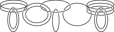
Figure 7. An example of Lickorish’s surgery link.

Remark 3.3.

Conversely, a surgery presentation can be converted to a Heegaard splitting. For instance, Lu’s method in [Lu92] tells us how to obtain a Heegaard splitting from a surgery link, as a product of explicit Dehn twists on an explicit surface. By rewriting those Dehn twists in terms of the Lickorish twists, for instance by following the arguments of existing proofs that Lickorish twists generate the mapping class group (e.g, see [Lic62, Lic64] or [FM12]), one would obtain a word in the Lickorish twists which represents the mapping class, and in turn an upper bound for the Heegaard-Lickorish complexity of the 3-manifold. We do not address details here.

Remark 3.4.

Theorem 3.2 and (the proof of) Theorem B immediately give a triangulation from a Heegaard splitting, together with the following complexity estimate:

$$c^{\text{simp}}(M)\leq 72\cdot(2\cdot c^{\text{HL}}(M)^{2}+3\cdot c^{\text{HL}}(M)).$$

It tells us that the simplicial complexity is bounded by a quadratic function in the Heegaard-Lickorish complexity. A quadratic bound seems to be the best possible result from this method (unless one finds a clever simplification of the resulting surgery link). For instance, by generalizing the rightmost 5 components in Figure 7 and considering the corresponding mapping class, one sees that there is actually a genus one mapping class of Lickorish word length $\leq\ell$ for which the associated link $L$ has crossing number $\geq\frac{\ell}{2}(\frac{\ell}{2}-1)$. In general, except for sufficiently small values of $c^{\text{HL}}$, this quadratic bound is weaker than the linear bound in Theorem A.

Remark 3.5.

The upper bound to the (pseudo-)simplicial complexity in terms of Heegaard splittings given in Theorem A is often stronger than Matveev’s upper bound in [Mat90, Mat07]. We recall Matveev’s result: suppose $M$ admits a Heegaard splitting $M=H_{1}\cup_{\Sigma}H_{2}$ with handlebodies $H_{1}$ and $H_{2}$ and Heegaard surface $\Sigma$. Let $\alpha$ and $\beta$ be the union of the meridian curves of $H_{1}$ and $H_{2}$ on $\Sigma$, respectively. Suppose $\alpha$ and $\beta$ are transverse, $n=\#(\alpha\cap\beta)$, and the closure of a component of $\Sigma\smallsetminus(\alpha\cup\beta)$ contains $m$ points in $\alpha\cap\beta$. Then $c(M)\leq n-m$ [Mat90, Proposition 3], [Mat07, Proposition 2.1.8]. As an explicit example, let $\tau$, $\sigma$ be the $+1$ Dehn twists along the meridian and preferred longitude on the boundary of the standard solid torus in $S^{3}$, and consider the lens space $L$ with Heegaard splitting determined by the mapping class of $\sigma^{k}\tau^{k}$. It is straightforward to see that $n=k^{2}+1$ and $m=4$ for this Heegaard splitting, so that the result in [Mat90, Mat07] gives $c(L)\leq k^{2}-3$, a quadratic upper bound. On the other hand, Theorem A gives a linear upper bound $c(L)\leq c^{\text{simp}}(L)\leq 1104k$, since $\sigma^{k}\tau^{k}$ has Lickorish word length $\leq 2k$. In fact, for arbitrary $N>0$, we can construct examples of lens spaces, using mapping classes of the form $(\sigma^{k}\tau^{k})^{N}$ and $\tau^{k}(\sigma^{k}\tau^{k})^{N}$, for which Matveev’s upper bound $c(M)\leq n-m$ has order $N$ (i.e., asymptotic growth of $k^{N}$) while Theorem A gives a linear upper bound.

The rest of this section is devoted to the proof of Theorem A. The key idea used in our proof below, which enables us to produce a more efficient triangulation (cf. Remark 3.4), is that we view Lickorish’s surgery link (Figure 7) as a link in the thickened Heegaard surface.

Proof of Theorem A.

Here we will prove the following statement, which is slightly sharper than Theorem A: if a closed $3$-manifold $M\neq S^{3}$ has Heegaard-Lickorish complexity $\ell$, then the simplicial complexity of $M$ is not greater than $552\ell-120$.

Suppose $h\in\operatorname{Mod}(\Sigma_{g})$ gives a Heegaard splitting of a given $3$-manifold $M$, and suppose $h$ is a product of $\ell$ Lickorish generators. Both $g$ and $\ell$ are nonzero, since $M\neq S^{3}$. By Lickorish [Lic62], $M$ is obtained by surgery on an $\ell$-component link $L$ in $S^{3}$, where each component has either $(+1)$ or $(-1)$-framing. His proof tells us more about $L$ (another useful reference for this is [Rol76, Chapter 9, Section I]). In fact, $L$ lies in a bicollar $\Sigma_{g}\times[-1,1]$ of $\Sigma_{g}$ in $S^{3}$, and each component is of the form $\alpha_{i}\times\{t\}$, $\beta_{i}\times\{t\}$, or $\gamma_{i}\times\{t\}$ for some $i$ and $t\in[-1,1]$. An example is shown in Figure 7. Let

$$D=\Big{(}\bigcup_{i=1}^{g}\alpha_{i}\Big{)}\cup\Big{(}\bigcup_{i=1}^{g}\beta_{i}\Big{)}\cup\Big{(}\bigcup_{i=1}^{g-1}\gamma_{i}\Big{)}.$$

Then $L$ lies on $D\times[-1,1]\subset S^{3}$.

Note that for a link in the bicollar $\Sigma_{g}\times[-1,1]$, if each component is regular with respect to the projection of $\Sigma_{g}\times[-1,1]\mathchoice{\longrightarrow}{\rightarrow}{\rightarrow}{\rightarrow}\Sigma_{g}$, then the blackboard framing with respect to $\Sigma_{g}$ is well-defined; the preferred parallel with respect to the blackboard framing is defined to be the push-off along the $[-1,1]$ direction. In particular, for our surgery link $L$, the blackboard framing with respect to $\Sigma_{g}$ is equal to the zero framing in $S^{3}$.

Now, in order to construct a triangulation of $\Sigma_{g}\times[-1,1]\smallsetminus\nu(L)$, we proceed similarly to the proof of Lemma 2.1; the difference is that we now use a “diagram” on $\Sigma_{g}$, instead of a planar link diagram. Let $G_{0}$ be the dual graph of $D$ on $\Sigma_{g}$. Let $G$ be the graph shown in Figure 8, which is obtained by adding parallel edges to $G_{0}$.

(top view) at 171 131 (bottom view) at 171 5 $D$ at 90 200 $G$ at 80 162 $D$ at 90 73 $G$ at 80 100

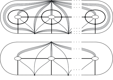
Figure 8. The graphs $D$ and $G$ on $\Sigma_{g}$, which are depicted in thick and thin edges respectively.

Note that for each of the curves $\alpha_{i}$, $\beta_{i}$ and $\gamma_{i}$, an edge of $G_{0}$ dual to the curve is chosen and two parallels of the chosen edge are added to produce $G$. Each region of $G$ is a quadrangle or a bigon. (Each quadrangle/bigon has no two edges which are identified, while vertices are allowed to be identified; using this, it can be verified that our construction described below gives a simplicial complex structure in which each tetrahedron has no identified vertices and is uniquely determined by its vertices.)

Cutting $\Sigma_{g}\times[-1,1]\smallsetminus\nu(L)$ along $G\times[-1,1]$, we obtain pieces corresponding to quadrangle regions and bigon regions; call them type (i) and (ii) respectively. See the left of Figure 9. Cutting along $D\times[-1,1]$, a type (i) piece is divided into four cubic subpieces, and a type (ii) piece is divided into two triangular prism subpieces. See the middle of Figure 9. Hatched quadrangles represent $\partial\nu(L)$.

$=$ a cone of at 235 250 $=$ a cone of at 235 70 type (i) at 90 160 type (ii) at 90 15

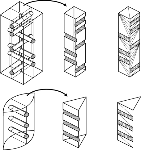
Figure 9. Decomposition of the surgery link exterior pieces.

For a type (i) subpiece, triangulate the three front faces of each subpiece as in the top right of Figure 9, and then triangulate the subpiece by taking a cone at the opposite vertex, as we did in the proof of Lemma 2.1. We claim that there are $6k+6$ tetrahedra in this subpiece triangulation, where $k$ is the number of hatched quadrangles in the subpiece. The number of tetrahedra in the subpiece is equal to the number of triangles in the three front faces. There are two triangles in the top face. To count triangles in the remaining two faces, observe that the front middle vertical edge is divided into $2k+1$ $1$-simplices. There are $4k+2$ triangles that have one of these $1$-simplices as an edge, and there are $2k+2$ remaining triangles. Therefore there are total $6k+6$ triangles, as we claimed.

A type (ii) subpiece is triangulated similarly, as depicted in the bottom of Figure 9. When a type (ii) subpiece has $k$ hatched quadrangles, its triangulation has $4k+3$ tetrahedra.

Combining the triangulations of the subpieces, we obtain a triangulation of $\Sigma_{g}\times[-1,1]\smallsetminus\nu(L)$. To estimate the number of tetrahedra, first observe that the graph $D$ has $3g-2$ vertices, where $g$ is the genus of the Heegaard surface $\Sigma_{g}$. Therefore its dual graph $G_{0}$ has $3g-2$ quadrangular regions. Since $2(3g-1)$ parallel edges have been added to $G_{0}$ and each of them introduces a bigon region, the graph $G$ has $3g-2$ quadrangular regions and $6g-2$ bigon regions. It follows that there are $12g-8$ type (i) subpieces and $12g-4$ type (ii) subpieces in $\Sigma_{g}\times[-1,1]\smallsetminus\nu(L)$. Also, observe that each component of $L$ passes through type (i) pieces at most three times, and type (ii) pieces twice. Therefore a component can contribute at most $4\cdot 3=12$ hatched quadrangles in type (i) subpieces, and $2\cdot 2=4$ hatched quadrangles in type (ii) subpieces. It follows that there are at most

$$6\cdot 12\ell+6\cdot(12g-8)+4\cdot 4\ell+3\cdot(12g-4)=88\ell+108g-60$$

tetrahedra in our triangulation of $\Sigma_{g}\times[-1,1]\smallsetminus\nu(L)$.

For later use, note that our triangulation restricted to $\Sigma_{g}\times\{t\}$ ($t=\pm 1$) has $2(12g-8)+(12g-4)=36g-20$ triangles, since the top face of each of the $12g-8$ type (i) subpieces consists of two triangles, and the top of each of the $12g-4$ type (ii) subpieces is a single triangle.

Now we triangulate the inner and outer handlebodies, which are the components of $S^{3}\smallsetminus(\Sigma_{g}\times(-1,1))$. First we consider the outer handlebody. Choose disjoint disks $D_{0},D_{1},\ldots,D_{g}$ in the outer handlebody such that $\partial D_{i}=\alpha_{i}$ for $i=1,\ldots,g$, and $\partial D_{0}$ is the union of the outermost edges of the graph $G$ in the top view of Figure 8; $\partial D_{0}$ is parallel to the outer dotted circle in Figure 8. Our triangulation on $\Sigma_{g}\times\{1\}$ divides $\partial D_{0}$ into $2g$ edges, each of $\partial D_{1}$ and $\partial D_{g}$ into 6 edges, and each $\partial D_{i}$ ($i=2,\ldots,g-1$) into 8 edges. Extending this triangulation of the boundary, we triangulate $D_{0}$ into $2g-2$ triangles, each of $D_{1}$, $D_{g}$ into 4 triangles, and each $D_{i}$ ($i=2,\ldots,g-1$) into 6 triangles, by drawing edges joining vertices. Cutting the outer handlebody along the disks $D_{0}$, $\ldots$, $D_{g}$, we obtain two $3$-balls $B_{1}$ and $B_{2}$. Our triangulations of the $D_{i}$ and $\Sigma_{g}\times\{1\}$ give triangulations of $\partial B_{1}$ and $\partial B_{2}$. Triangulate each of $B_{1}$ and $B_{2}$ by taking the cone of the boundary. Note that a triangle in $\Sigma\times\{1\}$ contributes one tetrahedron to $B_{1}\cup B_{2}$, while a triangle in $D_{i}$ contributes two tetrahedra to $B_{1}\cup B_{2}$. It follows that the outer handlebody has at most $(36g-20)+2\cdot(2g-2+6g-4)=52g-32$ tetrahedra.

For the inner handlebody, choose disjoint disks $D^{\prime}_{1},\ldots,D^{\prime}_{g},D^{\prime\prime}_{1},\ldots,D^{\prime\prime}_{g-1}$ in the inner handlebody such that $\partial D^{\prime}_{i}=\beta_{i}$ and $\partial D^{\prime\prime}_{i}=\gamma_{i}$. Similarly to the case of the disks $D_{i}$ above, our triangulation extends to $(\bigcup D^{\prime}_{i})\cup(\bigcup D^{\prime\prime}_{j})$ where $D^{\prime}_{i}$ and $D^{\prime\prime}_{i}$ are decomposed to 2 and 4 triangles respectively. Cutting the inner handlebody along the disks $D^{\prime}_{i}$ and $D^{\prime\prime}_{i}$, we obtain $g$ 3-balls. Triangulate each 3-ball by taking the cone of the boundary. A counting argument similar to the above shows that the inner handlebody has $(36g-20)+2(2g+4(g-1))=48g-28$ tetrahedra.

To obtain the surgery manifold, attach and triangulate Dehn filling tori as in the proof of Lemma 2.1. Recall that the blackboard framing is equal to the zero framing in the present case. Since each component of $L$ passes through two type (ii) pieces each of which introduces a half twist with respect to the blackboard framing, each Dehn filling torus can be assumed to be attached along the given $(\pm 1)$-framing of $L$, by appropriately choosing diagonal edges used to triangulate the hatched quadrangles of type (ii) pieces in Figure 9. Therefore the surgery manifold is equal to the given $M$. Since there are at most $16\ell$ hatched quadrangles and each hatched quadrangle contributes a triangular prism which consists of $3$ tetrahedra in the Dehn filling tori, there are at most $48\ell$ tetrahedra in the Dehn filling tori.

It follows that our triangulation of the surgery manifold $M$ has at most

$$(88\ell+108g-60)+(52g-32)+(48g-28)+48\ell=136\ell+208g-120$$

tetrahedra. By Lemma 3.1, we may assume that $g\leq 2\ell$. It follows that the simplicial complexity of $M$ is at most $552\ell-120$. ∎

4. Theorems A and B are asymptotically optimal

In this section we prove Theorem D and related results. For this purpose we use some results in [Cha16b]. First, we need the following lower bound of the simplicial complexity. In [CG85], Cheeger and Gromov introduced the von Neumann $L^{2}$ $\rho$-invariant $\rho^{(2)}(M,\phi)\in\mathbb{R}$ which is defined for a smooth closed $(4k-1)$-manifold $M$ and a homomorphism $\phi\colon\pi_{1}(M)\mathchoice{\longrightarrow}{\rightarrow}{\rightarrow}{\rightarrow}G$. By deep analytic arguments, they showed that for each $M$ there is a universal bound for the values of $\rho(M,\phi)$ [CG85]; that is, there is $C_{M}>0$ satisfying that $|\rho^{(2)}(M,\phi)|\leq C_{M}$ for any $\phi$. In [Cha16b], a topological approach to the universal bound for $\rho^{(2)}(M,\phi)$ is presented, and in particular, an explicit linear universal bound is given in terms of the simplicial complexity of 3-manifolds:

Theorem 4.1 ([Cha16b, Theorem 1.5]).

Suppose $M$ is a closed 3-manifold. Then

$$|\rho^{(2)}(M,\phi)|\leq 363090\cdot c^{\text{simp}}(M)$$

for any homomorphism $\phi$.

In this paper, we will use the Cheeger-Gromov $\rho$-invariant as a lower bound of the simplicial complexity.

For the lens space $L(n,1)$ and the identity map $\mathrm{id}\colon\pi_{1}(L(n,1))\mathchoice{\longrightarrow}{\rightarrow}{\rightarrow}{\rightarrow}\mathbb{Z}_{n}$ ($n>0$), Lemma 7.1 of [Cha16b] gives the following value of the Cheeger-Gromov $\rho$-invariant, using the computation of Atiyah-Patodi-Singer [APS75, p. 412]:

$$\rho^{(2)}(L(n,1)),\mathrm{id})=\frac{n}{3}+\frac{2}{3n}-1.$$

From this and Theorem 4.1, a lower bound of the simplicial complexity of $L(n,1)$ is obtained. We state it as a lemma:

Lemma 4.2.

$\displaystyle c^{\text{simp}}(L(n,1))\geq\frac{n-3}{1089270}.$

We remark that a pseudo-simplicial complexity analogue is given in [Cha16b, Corollary 1.15].

Now we are ready to proof Theorem D. In fact, the following stronger inequalities hold, and Theorem D follows immediately from them.

Theorem 4.3.

$$\frac{1}{1089720}\cdot\Big{(}1-\frac{3}{n}\Big{)}\cdot c^{\text{HL}}(L(n,1))\leq c^{\text{simp}}(L(n,1)),$$

$$\frac{1}{1089720}\cdot\Big{(}1-\frac{3}{n}\Big{)}\cdot c^{\text{surg}}(L(n,1))\leq c^{\text{simp}}(L(n,1)).$$

Proof.

Since $L(n,1)$ is obtained by the $n$-framed surgery on the unknot, it is easily seen that $c^{\text{HL}}(M)$, $c^{\text{surg}}(M)\leq n$. The desired inequalities follow from this and Lemma 4.2. ∎

In what follows we discuss a generalization and a specialization of the lens space case we considered in Theorem 4.3.

First, the second inequality in Theorem 4.3 generalizes for a larger class of 3-manifolds. For a knot $K$ in $S^{3}$, let $M(K,n)$ be the 3-manifold obtained by $n$-framed surgery on $K$. Let $g_{4}(K)$ be the (topological) slice genus of $K$.

Theorem 4.4.

For any $n\neq 0$,

$$\frac{1}{1089720}\cdot\Big{(}1-\frac{3+6g_{4}(K)}{|n|}\Big{)}\cdot\big{(}c^{\text{surg}}(M(K,n))-2c(K)\big{)}\leq c^{\text{simp}}(M(K,n)).$$

Proof.

Let $\phi\colon\pi_{1}(M(K,n))\mathchoice{\longrightarrow}{\rightarrow}{\rightarrow}{\rightarrow}\mathbb{Z}_{|n|}$ be the abelianization. Due to [Cha16a, Equation (2.8)],

$$|\rho^{(2)}(M(K,n),\phi)|\geq\frac{1}{3}\cdot(|n|-3-6g_{4}(K)).$$

By Theorem 4.1, it follows that

(4.1) $$c^{\text{simp}}(M(K,n))\geq\frac{1}{1089270}\cdot(|n|-3-6g_{4}(K)).$$

By definition, $c^{\text{surg}}(M(K,n))\leq 2c(K)+|n|$. From this and (4.1), the desired inequality follows. ∎

On the other hand, if we consider the special case of lens spaces $L(2k,1)$, then the inequalities in Theorem 4.3 (and hence those in Theorem D) can be improved significantly as follows.

Theorem 4.5.

For $k>1$, the following hold:

$$\Big{(}1-\frac{3}{2k\mathstrut}\Big{)}\cdot c^{\text{HL}}(L(2k,1))\leq c^{\text{simp}}(L(2k,1)),$$

$$\Big{(}1-\frac{3}{2k}\Big{)}\cdot c^{\text{surg}}(L(2k,1))\leq c^{\text{simp}}(L(2k,1)).$$

Proof.

Due to Jaco, Rubinstein, and Tillman [JRT09], the pseudo-simplicial complexity of $L(2k,1)$ is equal to $2k-3$ for $k>1$, and consequently $c^{\text{simp}}(L(2k,1))\geq 2k-3$. Using this in place of Lemma 4.2 in the proof of Theorem 4.3, we obtain the inequalities. ∎

We finish this section with a proof of Theorem C.

Proof of Theorem C.

Recall the definition of the “largest possible value” of the simplicial complexity for Heegaard-Lickorish complexity $\leq\ell$:

$$s_{\text{HL}}(\ell):=\sup\{c^{\text{simp}}(M)\mid c^{\text{HL}}(M)\leq\ell\}.$$

The first assertion of Theorem C, which says $s_{\text{HL}}(\ell)\in O(\ell)\cap\Omega(\ell)$, follows immediately from the estimate

(4.2) $$\frac{1}{1089270}\leq\limsup_{\ell\mathchoice{\longrightarrow}{\rightarrow}{\rightarrow}{\rightarrow}\infty}\frac{s_{\text{HL}}(\ell)}{\ell}\leq 552.$$

which we prove in what follows.

Fix $\ell$. For any $M$ with $c^{\text{HL}}(M)\leq\ell$, we have

$$\frac{c^{\text{simp}}(M)}{\ell}\leq\frac{c^{\text{simp}}(M)}{c^{\text{HL}}(M)}\leq 552$$

by Theorem A. Taking the supremum over all such $M$, we obtain $s_{\text{HL}}(\ell)/\ell\leq 552$. From this we obtain the upper bound in (4.2).

By the definition of $s_{\text{HL}}(\ell)$, we have

$$\frac{c^{\text{simp}}(M)}{c^{\text{HL}}(M)}\leq\frac{s_{\text{HL}}(c^{\text{HL}}(M))}{c^{\text{HL}}(M)}$$

for any $M$. By Theorem 4.3, the limit supremum of the left hand side as $c^{\text{HL}}(M)\mathchoice{\longrightarrow}{\rightarrow}{\rightarrow}{\rightarrow}\infty$ is bounded from below by $1/1089270$. From this the lower bound in (4.2) follows.

The analogous statement for the function $s_{\text{surg}}(k)$ is proved by the same argument. ∎

References

- [APS75] M. F. Atiyah, V. K. Patodi, and I. M. Singer, Spectral asymmetry and Riemannian geometry. II, Math. Proc. Cambridge Philos. Soc. 78 (1975), no. 3, 405–432.
- [CG85] Jeff Cheeger and Mikhael Gromov, Bounds on the von Neumann dimension of -cohomology and the Gauss-Bonnet theorem for open manifolds, J. Differential Geom. 21 (1985), no. 1, 1–34.
- [Cha16a] Jae Choon Cha, Complexity of surgery manifolds and Cheeger-Gromov invariants, Int. Math. Res. Not. IMRN (2016), no. 18, 5603–5615.
- [Cha16b] by same author, A topological approach to Cheeger-Gromov universal bounds for von Neumann -invariants, Comm. Pure Appl. Math. 69 (2016), no. 6, 1154–1209.
- [CL] Jae Choon Cha and Charles Livingston, KnotInfo: table of knot invariants, http://www.indiana.edu/~knotinfo.
- [FM12] Benson Farb and Dan Margalit, A primer on mapping class groups, Princeton Mathematical Series, vol. 49, Princeton University Press, Princeton, NJ, 2012.
- [JRT09] William Jaco, Hyam Rubinstein, and Stephan Tillmann, Minimal triangulations for an infinite family of lens spaces, J. Topol. 2 (2009), no. 1, 157–180.
- [JRT11] William Jaco, J. Hyam Rubinstein, and Stephan Tillmann, Coverings and minimal triangulations of 3-manifolds, Algebr. Geom. Topol. 11 (2011), no. 3, 1257–1265.
- [JRT13] by same author, -Thurston norm and complexity of -manifolds, Math. Ann. 356 (2013), no. 1, 1–22.
- [Lic62] W. B. R. Lickorish, A representation of orientable combinatorial -manifolds, Ann. of Math. (2) 76 (1962), 531–540.
- [Lic64] by same author, A finite set of generators for the homeotopy group of a -manifold, Proc. Cambridge Philos. Soc. 60 (1964), 769–778.
- [Lu92] Ning Lu, A simple proof of the fundamental theorem of Kirby calculus on links, Trans. Amer. Math. Soc. 331 (1992), no. 1, 143–156.
- [Mat90] Sergei Matveev, Complexity theory of three-dimensional manifolds, Acta Appl. Math. 19 (1990), no. 2, 101–130.
- [Mat03] by same author, Complexity of three-dimensional manifolds: problems and results [translated from proceedings of the conference “geometry and applications” dedicated to the seventieth birthday of v. a. toponogov (russian) (novosibirsk, 2000), 102–110, Ross. Akad. Nauk Sib. Otd. Inst. Mat., Novosibirsk, 2001], Siberian Adv. Math. 13 (2003), no. 3, 95–103.
- [Mat07] by same author, Algorithmic topology and classification of 3-manifolds, second ed., Algorithms and Computation in Mathematics, vol. 9, Springer, Berlin, 2007.
- [MPV09] Sergei Matveev, Carlo Petronio, and Andrei Vesnin, Two-sided asymptotic bounds for the complexity of some closed hyperbolic three-manifolds, J. Aust. Math. Soc. 86 (2009), no. 2, 205–219.
- [Rol76] Dale Rolfsen, Knots and links, Publish or Perish Inc., Berkeley, Calif., 1976, Mathematics Lecture Series, No. 7.
- [Wee05] Jeff Weeks, Computation of hyperbolic structures in knot theory, Handbook of knot theory, Elsevier B. V., Amsterdam, 2005, pp. 461–480.