Lagrangian Duality in 3D SLAM:
Verification Techniques and Optimal Solutions

Abstract

State-of-the-art techniques for simultaneous localization and mapping (SLAM) employ iterative nonlinear optimization methods to compute an estimate for robot poses. While these techniques often work well in practice, they do not provide guarantees on the quality of the estimate. This paper shows that Lagrangian duality is a powerful tool to assess the quality of a given candidate solution. Our contribution is threefold. First, we discuss a revised formulation of the SLAM inference problem. We show that this formulation is probabilistically grounded and has the advantage of leading to an optimization problem with quadratic objective. The second contribution is the derivation of the corresponding Lagrangian dual problem. The SLAM dual problem is a (convex) semidefinite program, which can be solved reliably and globally by off-the-shelf solvers. The third contribution is to discuss the relation between the original SLAM problem and its dual. We show that from the dual problem, one can evaluate the quality (i.e., the suboptimality gap) of a candidate SLAM solution, and ultimately provide a certificate of optimality. Moreover, when the duality gap is zero, one can compute a guaranteed optimal SLAM solution from the dual problem, circumventing non-convex optimization. We present extensive (real and simulated) experiments supporting our claims and discuss practical relevance and open problems.

Please cite this paper as: “L. Carlone, D.M. Rosen, G.C. Calafiore, J.J. Leonard, F. Dellaert, Lagrangian Duality in 3D SLAM: Verification Techniques and Optimal Solutions, Int. Conf. on Intelligent RObots and Systems (IROS), 2015.”

I Introduction

Simultaneous localization and mapping (SLAM) is an enabling technology for many applications, including service and industrial robotics, autonomous driving, search and rescue, planetary exploration, and augmented reality.

The last decade has witnessed several groundbreaking results in SLAM, and state-of-the-art approaches are now transitioning from academic research to industrial applications. Standard techniques compute an estimate (e.g., for robot poses) by minimizing a nonlinear cost function, whose global minimum is the maximum likelihood estimate (or maximum a posteriori estimate in presence of priors). The optimization problem underlying SLAM is commonly solved using iterative nonlinear optimization methods, e.g. the Gauss-Newton method [1, 2, 3], the gradient method [4, 5], trust region methods [6], or ad-hoc approximations [7, 8].

Despite the success of state-of-the-art techniques, some practical and theoretical problems remain open. While iterative approaches are observed to work well in many problem instances, they cannot guarantee the correctness (global optimality) of the estimates that they compute. This is due to the fact that the optimization problem is non-convex, hence iterative techniques may be trapped in local minima (Fig. 1), which correspond to wrong estimates. Recent work [9, 10] shows that iterative techniques fail to converge to a correct estimate even in fairly simple (real and simulated) 3D problems. Recent research efforts have addressed the issue of global convergence from several angles. Olson et al. [4], Grisetti et al. [5], Rosen et al. [6], and Tron et al. [11] study iterative techniques with larger basins of convergence. Carlone et al. [8, 12], and Rosen et al. [10] propose initialization techniques to bootstrap iterative optimization. Huang et al. [13], Wang et al. [14], Carlone [15], and Khosoussi et al. [16] investigate the factors influencing local convergence and the quality of the optimal SLAM solution. While these techniques provide remarkable insights into the problem, and working solutions to improve convergence, none of them can guarantee the recovery of a globally optimal solution to SLAM.

	sphere-a	torus
Optimum
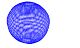
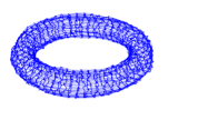
Local Minimum

Figure 1: This paper exploits Lagrangian duality to evaluate the quality of a SLAM solution. For instance, our verification techniques are able to certify the optimality of the solutions in the first row of the figure, while they reject as suboptimal the estimates shown in the bottom row.

The motivation behind this work is that the transition of SLAM from research topic to industrial technology requires techniques with guaranteed performance. In autonomous vehicle applications, failure to produce a correct SLAM solution may put passengers’ lives at risk. In other applications, SLAM failures can possibly cascade into path planning failures (if the plan is computed using a wrong map), and this may prevent the reliable operation of mobile robots.

Therefore, in this paper we address the following question:

Verification Problem: Given a candidate SLAM estimate (e.g., returned by a state-of-the-art iterative solver), is it possible to evaluate the quality of this estimate (e.g., its sub-optimality gap), possibly certifying its optimality?

To address this problem, we introduce a powerful tool, Lagrangian duality, borrowing the corresponding theory from the optimization community. Duality was first applied to 2D SLAM by Carlone and Dellaert [9]. In this work, we provide a nontrivial extension of [9] to 3D SLAM.

This paper contains three main contributions. The first contribution is a revised formulation of the SLAM inference problem. Our formulation is a probabilistically grounded maximum likelihood (ML) estimator, and has the advantage of leading to an optimization problem with quadratic objective, which facilitates the derivation of the dual problem. Our revised SLAM formulation is presented in Section II.

The second contribution is the derivation of the Lagrangian dual problem. A key step towards this goal consists of rewriting the 3D SLAM problem as a quadratic optimization problem with quadratic equality constraints. Intuitively, the constraints impose that the pose estimates are members of $\mathrm{SE}(3)$, while the objective minimizes the mismatch w.r.t. the measurements. The dual SLAM problem, introduced in Section III, is a (convex) semidefinite program (SDP), and can be solved globally by off-the-shelf solvers.

The third contribution is to provide verification techniques to assess the quality of a given SLAM solution, leveraging the relation between the standard SLAM problem and its dual. We show that solving the dual problem allows us to bound the sub-optimality gap of a given candidate solution, hence we are able to quantify how far the candidate solution is from being optimal. Since current SDP solvers do not scale well to large problems, we also propose a second verification technique that does not require solving the SDP. As a by-product of our derivation, we show that, when the duality gap is zero, we can compute an optimal SLAM solution directly from the dual problem. Our verification techniques, presented in Section IV, can be seamlessly integrated in standard SLAM pipelines. Experimental evidence (Section V) confirms that these techniques enable the certification of globally optimal solutions in both real and simulated experiments. Extra results and visualizations are given in the appendix of this paper.

II 3D Pose Graph Optimization Revisited

We consider the pose graph optimization (PGO) formulation of the SLAM problem. PGO computes the maximum likelihood estimate for $n$ poses ${\bm{x}}_{1},\ldots,{\bm{x}}_{n}$, given $m$ relative pose measurements ${\bar{{\bm{x}}}}_{ij}$ between pairs of poses $i$ and $j$. In a 3D setup, both the unknown poses and the measurements are quantities in $\mathrm{SE}(3)\doteq\{({\bm{R}},{\bm{t}}):{\bm{R}}\in\mathrm{SO}(3),{\bm{t}}\in{{\mathbb{R}}^{3}}\}$. We use the notation ${\bm{x}}_{i}\!=\!({\bm{R}}_{i},{\bm{t}}_{i})$ and ${\bar{{\bm{x}}}}_{ij}\!=\!(\bar{{\bm{R}}}_{ij},\bar{{\bm{t}}}_{ij})$ to make explicit the rotation and the translation of each pose. PGO can be visualized as a directed graph ${\cal G}({\cal V},{\cal E})$, in which we associate a node $i\in{\cal V}\!=\!\{1,\!\ldots\!,n\}$ to each pose ${\bm{x}}_{i}$ and an edge $(i,j)\!\in\!{\cal E}$ to each relative measurement ${\bar{{\bm{x}}}}_{ij}$.

In this section we propose a revised PGO formulation. The key difference w.r.t. related work is the use of the chordal distance to quantify the rotation errors (more details in Section II-B). To lay the groundwork for this formulation, we begin with a generative model for our measurements, and then derive the corresponding ML estimator.

II-A Generative Noise Model

We assume the following generative model for the relative pose measurements $(\bar{{\bm{R}}}_{ij},\bar{{\bm{t}}}_{ij})$:

$$\begin{array}[]{llllll}\bar{{\bm{t}}}_{ij}\!\!\!&=&\!\!\!{\bm{R}}_{i}^{\mathsf{T}}({\bm{t}}_{j}\!-\!{\bm{t}}_{i})\!+\!{\bm{t}}_{\epsilon}&\;\;{\bm{t}}_{\epsilon}\;\sim\mbox{gaussian}({\mathbf{0}}_{3},{\tiny\omega_{t}^{2}}{\mathbf{I}}_{3})\\ \bar{{\bm{R}}}_{ij}\!\!\!&=&\!\!\!{\bm{R}}_{i}^{\mathsf{T}}{\bm{R}}_{j}{\bm{R}}_{\epsilon}&\;\;{\bm{R}}_{\epsilon}\sim\mbox{vonMises}({\mathbf{I}}_{3},{\tiny\omega_{R}^{2}})\end{array}$$ (1)

where “$\mbox{gaussian}({\bm{\mu}},{\bm{\Omega}})$” denotes a Gaussian distribution with mean ${\bm{\mu}}$ and information matrix ${\bm{\Omega}}$, while “$\mbox{vonMises}({\bm{S}},\kappa)$” denotes the isotropic von Mises-Fisher distribution, with mean ${\bm{S}}\in\mathrm{SO}(3)$ and concentration parameter $\kappa$. The key difference w.r.t. to measurement models in other PGO formulations lies in the use of the von Mises-Fisher distribution as the model for the rotational measurements errors ${\bm{R}}_{\epsilon}\in\mathrm{SO}(3)$.

The isotropic von Mises-Fisher (or Langevin) [17] distribution on $\mathrm{SO}(n)$ with mean ${\bm{S}}\in\mathrm{SO}(n)$ and concentration parameter $\kappa\geq 0$ can be written explicitly as:

$${\mathbb{P}}\left({\bm{R}}_{\epsilon}\right)=\frac{1}{c_{n}(\kappa)}\exp\left(\kappa\;\mathrm{tr}\left({\bm{S}}^{\mathsf{T}}{\bm{R}}_{\epsilon}\right)\right),$$ (2)

where $\mathrm{tr}\left(\cdot\right)$ is the matrix trace and $c_{n}(\kappa)$ is a normalization term. Closed-form expressions for $c_{n}(\kappa)$ are given in [17]; these are inconsequential for our derivation. For $\kappa\rightarrow 0$, the distribution tends to the uniform distribution over $\mathrm{SO}(n)$. For $\kappa\rightarrow\infty$, ${\bm{R}}_{\epsilon}={\bm{S}}$ with probability one. Roughly speaking, one may think at $\kappa$ in terms of information content.

We are now ready to introduce the maximum likelihood estimator for the poses, given the measurement model (1).

II-B Maximum Likelihood Estimator

The ML estimate corresponds to the set of poses maximizing the likelihood of the measurements, or, equivalently, minimizing the negative log-likelihood:

$$f_{\tt ML}^{\star}=\min_{\{{\bm{x}}_{i}\in\mathrm{SE}(3)\}}\displaystyle\sum_{(i,j)\in{\cal E}}-\log{\cal L}(\bar{{\bm{R}}}_{ij}|{\bm{x}})-\log{\cal L}(\bar{{\bm{t}}}_{ij}|{\bm{x}}).$$ (3)

The negative log-likelihood of the Cartesian measurements can be easily computed from the Gaussian distribution:

$$-\log{\cal L}(\bar{{\bm{t}}}_{ij}|{\bm{x}})={\tiny\omega_{t}^{2}}\left\|{\bm{t}}_{j}\!-\!{\bm{t}}_{i}\!-\!{\bm{R}}_{i}\bar{{\bm{t}}}_{ij}\right\|^{2}+\mbox{const.}$$ (4)

Using (2), the negative log-likelihood for $\bar{{\bm{R}}}_{ij}$ is:

$$\begin{split}-\log{\cal L}(\bar{{\bm{R}}}_{ij}|{\bm{x}})&=-{\tiny\omega_{R}^{2}}\;\mathrm{tr}\left({\bm{R}}_{j}^{\mathsf{T}}{\bm{R}}_{i}\bar{{\bm{R}}}_{ij}\right)+\mbox{const.}\\ &=\frac{{\tiny\omega_{R}^{2}}}{2}\left\|{\bm{R}}_{j}-{\bm{R}}_{i}\bar{{\bm{R}}}_{ij}\right\|^{2}_{{\tt F}}+\mbox{const.}\end{split}$$ (5)

where $\left\|\cdot\right\|^{2}_{{\tt F}}$ is the Frobenius matrix norm (sum of the squares of the entries), and we used $\left\|{\bm{S}}-{\bm{R}}\right\|^{2}_{{\tt F}}\!=\!\mathrm{tr}\left(({\bm{S}}\!-\!{\bm{R}})({\bm{S}}\!-\!{\bm{R}})^{\mathsf{T}}\right)$. The norm $\left\|{\bm{S}}-{\bm{R}}\right\|^{2}_{{\tt F}}$ is usually referred to as the chordal distance between two rotations ${\bm{S}}$ and ${\bm{R}}$ [18].

Plugging (4) and (5) back into (3) we obtain our ML estimator:

$$f_{\tt ML}^{\star}=\min_{\!\!\!\begin{subarray}{c}\{{\bm{t}}_{i}\in{{\mathbb{R}}^{3}}\}\\ \{{\bm{R}}_{i}\in\mathrm{SO}(3)\}\end{subarray}}\hskip 5.69046pt\displaystyle\sum_{(i,j)\in{\cal E}}\hskip 5.69046pt{\tiny\omega_{t}^{2}}\left\|{\bm{t}}_{j}\!-\!{\bm{t}}_{i}\!-\!{\bm{R}}_{i}\bar{{\bm{t}}}_{ij}\right\|^{2}\hskip 28.45274pt\text{(PGO)}$$

$$\hskip 85.35826pt+\frac{{\tiny\omega_{R}^{2}}}{2}\left\|{\bm{R}}_{j}\!-\!{\bm{R}}_{i}\bar{{\bm{R}}}_{ij}\right\|^{2}_{{\tt F}}\vspace{-0.1cm}$$ (6)

The main difference between (6) and formulations in related work is the use of the chordal distance (related work instead uses the geodesic distance $\left\|\mathrm{Log}\left(\bar{{\bm{R}}}_{ij}^{\mathsf{T}}{\bm{R}}_{i}^{\mathsf{T}}{\bm{R}}_{j}\right)\right\|^{2}$). References [9, 18] show that for small residual errors $\frac{1}{2}\left\|{\bm{R}}_{j}-{\bm{R}}_{i}\bar{{\bm{R}}}_{ij}\right\|^{2}_{{\tt F}}\approx\left\|\mathrm{Log}\left(\bar{{\bm{R}}}_{ij}^{\mathsf{T}}{\bm{R}}_{i}^{\mathsf{T}}{\bm{R}}_{j}\right)\right\|^{2}$, making the formulations equivalent from a practical standpoint.

The advantage of the formulation (6) is that it has a quadratic objective function. This facilitates the derivation of the Lagrangian dual problem, as shown in the next section.

III Lagrangian Duality in 3D PGO

The main goal of this paper is to provide tools to check if a candidate SLAM solution $\hat{{\bm{x}}}$ is globally optimal. If we knew the optimal cost $f_{\tt ML}^{\star}$ this would be easy: calling $f_{\tt ML}(\cdot)$ the objective function of (6), if $f_{\tt ML}(\hat{{\bm{x}}})=f_{\tt ML}^{\star}$ then $\hat{{\bm{x}}}$ is optimal. Unfortunately, $f_{\tt ML}^{\star}$ is unknown. Our contribution is to show that we can compute close proxies of $f_{\tt ML}^{\star}$ using duality theory. To make the derivation easier, we first rewrite the problem as a quadratic problem with equality constraints (Section III-A), and then derive the dual (Section III-B).

III-A Quadratic Problem with Quadratic Equality Constrains

In this section, we rewrite (6) in order to (i) have vector variables (the rotations ${\bm{R}}_{i}$ are matrices), and (ii) formulate the constraints ${\bm{R}}_{i}\in\mathrm{SO}(3)$ as quadratic equality constraints.

We define ${\bm{r}}_{i}\in{{\mathbb{R}}^{9}}$ as the vectorized version of ${\bm{R}}_{i}$: ${\bm{r}}_{i}\doteq[{\bm{R}}_{i}^{(1)}\;{\bm{R}}_{i}^{(2)}\;{\bm{R}}_{i}^{(3)}]^{\mathsf{T}}$, where ${\bm{R}}_{i}^{(k)}$ is the $k$th row of ${\bm{R}}_{i}$. We use the shorthand ${\bm{r}}_{i}=\mbox{rows}({\bm{R}}_{i})$ to obtain the vector representation ${\bm{r}}_{i}$ of a $3\times 3$ matrix ${\bm{R}}_{i}$. Using this parametrization, each summand in the objective in (6) becomes (using that $\|{\bm{R}}\|_{\tt F}=\|{\bm{R}}^{\mathsf{T}}\|_{\tt F}$ in the first expression):

$${\tiny\omega_{t}^{2}}\left\|{\bm{t}}_{j}\!-\!{\bm{t}}_{i}\!-\!{\bm{R}}_{i}\bar{{\bm{t}}}_{ij}\right\|^{2}+\frac{{\tiny\omega_{R}^{2}}}{2}\left\|{\bm{R}}_{j}^{\mathsf{T}}\!-\!\bar{{\bm{R}}}_{ij}^{\mathsf{T}}{\bm{R}}_{i}^{\mathsf{T}}\right\|^{2}_{{\tt F}}$$ (7)

$$= {\tiny\omega_{t}^{2}}\left\|{\bm{t}}_{j}\!-\!{\bm{t}}_{i}\!-\!{{\bm{T}}}_{ij}{\bm{r}}_{i}\right\|^{2}+\frac{{\tiny\omega_{R}^{2}}}{2}\left\|{\bm{r}}_{j}\!-\!{{\bm{Q}}}_{ij}{\bm{r}}_{i}\right\|^{2}\!\!\!\!\!\!$$

where ${{\bm{T}}}_{ij}\doteq{\mathbf{I}}_{3}\otimes\bar{{\bm{t}}}_{ij}^{\mathsf{T}}\in{{\mathbb{R}}^{3\times 9}}$, ${{\bm{Q}}}_{ij}\doteq{\mathbf{I}}_{3}\otimes\bar{{\bm{R}}}_{ij}^{\mathsf{T}}\in{{\mathbb{R}}^{9\times 9}}$, and $\otimes$ is the Kronecker product.

We cannot choose arbitrary vectors ${\bm{r}}_{i}\in{{\mathbb{R}}^{9}}$, but have to limit ourself to choices of ${\bm{r}}_{i}$ that produce meaningful rows of a rotation matrix ${\bm{R}}_{i}\in\mathrm{SO}(3)$. The rotation group $\mathrm{SO}(3)$ is defined as $\mathrm{SO}(3)\doteq\{{\bm{R}}\in{{\mathbb{R}}^{3\times 3}}\;{:}\;{\bm{R}}^{\mathsf{T}}{\bm{R}}={\mathbf{I}}_{3},\det({\bm{R}})=1\}$, which, written in terms of the rows of ${\bm{R}}_{i}$, becomes:

$${\bm{R}}_{i}^{\mathsf{T}}{\bm{R}}_{i}={\mathbf{I}}_{3}\!\! \!\!\Leftrightarrow\!\! \!\!({\bm{R}}_{i}^{(u)})^{\mathsf{T}}{\bm{R}}_{i}^{(v)}=\left\{\begin{array}[]{ll}1&\text{if }u=v,\\ 0&\text{if }u\neq v,\end{array}\right.\begin{array}[]{l}u,v=\\ 1,2,3\end{array}$$ (12)

$$\det({\bm{R}}_{i})=1\!\! \!\!\Leftrightarrow\!\! \!\!{\bm{R}}_{i}^{(1)}\times{\bm{R}}_{i}^{(2)}={\bm{R}}_{i}^{(3)}$$ (13)

where $\times$ is the cross product. In other words, the rows of a rotation matrix have to be orthonormal, and have to satisfy the right-hand rule. To derive the dual problem we relax the second condition ($\det({\bm{R}})=1$), which amounts to performing estimation in $\mathrm{O}(3)$ rather than $\mathrm{SO}(3)$ (i.e., resulting matrices can have determinant $\det({\bm{R}})=\pm 1$). Then in Proposition 4 we show how to reconcile our verification techniques to work directly on the original PGO problem (6).

Using (7) and (12) and relaxing the determinant constraints, we rewrite the PGO problem (6) as:

$$f^{\star}=\min_{\{{\bm{r}}_{i},{\bm{t}}_{i}\}}\!\!\! \!\!\!\!\displaystyle\sum_{(i,j)\in{\cal E}}\!\!{\tiny\omega_{t}^{2}}\left\|{\bm{t}}_{j}\!-\!{\bm{t}}_{i}\!-\!{{\bm{T}}}_{ij}{\bm{r}}_{i}\right\|^{2}+\frac{{\tiny\omega_{R}^{2}}}{2}\left\|{\bm{r}}_{j}\!-\!{{\bm{Q}}}_{ij}{\bm{r}}_{i}\right\|^{2}$$

subject to $$\left.\begin{array}[]{ll}{\bm{r}}_{i}^{\mathsf{T}}{\bm{E}}_{uv}{\bm{r}}_{i}=1,\quad u=v\\ {\bm{r}}_{i}^{\mathsf{T}}{\bm{E}}_{uv}{\bm{r}}_{i}=0,\quad u\neq v\end{array}\right\}\begin{array}[]{ll}u,v=1,2,3\\ i=1,\ldots,n\end{array}$$ (18)

where ${\bm{E}}_{uv}$ is a $9\times 9$ selection matrix composed of $3\times 3$ blocks that are zero everywhere except the $3\times 3$ block in position $(u,v)$, which is the identity matrix. The matrices ${\bm{E}}_{uv}$ are built such that ${\bm{r}}_{i}^{\mathsf{T}}{\bm{E}}_{uv}{\bm{r}}_{i}=({\bm{R}}_{i}^{(u)})^{\mathsf{T}}{\bm{R}}_{i}^{(v)}$, hence the constraints in (III-A) correspond to the orthonormality constraints in (12).

In order to write (III-A) in a more compact matrix notation, we define the vector $\breve{\bm{x}}=[{\bm{t}}_{1}^{\mathsf{T}},\ldots,{\bm{t}}_{n}^{\mathsf{T}},{\bm{r}}_{1}^{\mathsf{T}},\ldots,{\bm{r}}_{n}^{\mathsf{T}}]^{\mathsf{T}}\in{{\mathbb{R}}^{12n}}$. Using this notation, (III-A) becomes:

$$f^{\star}=\min_{\breve{\bm{x}}} \|\breve{{\bm{A}}}\breve{\bm{x}}\|^{2}\hskip 142.26378pt$$ (19)

subject to $$\left.\begin{array}[]{ll}\breve{\bm{x}}^{\mathsf{T}}\breve{{\bm{E}}}_{iuv}\breve{\bm{x}}=1,\quad u=v\\ \breve{\bm{x}}^{\mathsf{T}}\breve{{\bm{E}}}_{iuv}\breve{\bm{x}}=0,\quad u\neq v\end{array}\right\}\begin{array}[]{ll}u,v=1,2,3\\ i=1,\ldots,n\end{array}$$ (22)

where the matrices $\breve{{\bm{A}}}$ and $\breve{{\bm{E}}}_{iuv}$ are obtained by stacking the coefficient matrices in (III-A), with suitable zero blocks for padding; ${\tiny\omega_{t}^{2}}$ and ${\tiny\omega_{R}^{2}}$ are included in the definition of $\breve{{\bm{A}}}$.

Finally, since absolute poses are not observable from relative measurements, we fix a pose to be our reference frame. Without loss of generality we fix the pose of the first node to the identity pose (${\bm{t}}_{1}={\mathbf{0}}_{3}$ and ${\bm{R}}_{1}={\mathbf{I}}_{3}$, or, equivalently ${\bm{r}}_{1}=\mbox{rows}({\mathbf{I}}_{3})$). This process is usually called anchoring. Fixing the first pose modifies (19) as follows:

$$f^{\star}=\min_{{\bm{x}}} \left\|{\bm{A}}{\bm{x}}-{\bm{b}}\right\|^{2}\hskip 128.0374pt$$ (23)

subject to $$\left.\begin{array}[]{ll}{\bm{x}}^{\mathsf{T}}{{\bm{E}}}_{iuv}{\bm{x}}=1,\quad u=v\\ {\bm{x}}^{\mathsf{T}}{{\bm{E}}}_{iuv}{\bm{x}}=0,\quad u\neq v\end{array}\right\}\begin{array}[]{ll}u,v=1,2,3\\ i=1,\ldots,n-1\end{array}$$ (28)

where ${\bm{x}}\in{{\mathbb{R}}^{12(n-1)}}$ is obtained by removing the first pose from $\breve{{\bm{x}}}$, ${\bm{A}}$ is obtained by removing from $\breve{{\bm{A}}}$ the columns corresponding to the first pose, and ${\bm{b}}$ is the known right-hand-side arising from anchoring; ${{\bm{E}}}_{iuv}$ are the same as $\breve{{\bm{E}}}_{iuv}$ but without the rows and columns corresponding to the first pose.

We conclude this section by transforming (23) into an equivalent problem with homogeneous objective (i.e., without constant terms in the squared cost). For this purpose, we note that solving (23) is the same as solving:

$$f^{\star}=\min_{{\bm{x}},y} \left\|{\bm{A}}{\bm{x}}-{\bm{b}}y\right\|^{2}\hskip 56.9055pt\text{(primal problem)}$$

subject to $$\left.\begin{array}[]{ll}{\bm{x}}^{\mathsf{T}}{{\bm{E}}}_{iuv}{\bm{x}}=1,\quad u=v\\ {\bm{x}}^{\mathsf{T}}{{\bm{E}}}_{iuv}{\bm{x}}=0,\quad u\neq v\end{array}\right\}\begin{array}[]{ll}u,v=1,2,3\\ i=1,\ldots,n-1\end{array}$$ (33)

$$y^{2}=1\hskip 142.26378pt$$ (34)

meaning that the two problems have the same optimal objective, and the corresponding solutions can be mapped to each other. Intuitively, if the solution of (III-A) is $[{\bm{x}}_{H}^{\star}\;1]$, then ${\bm{x}}^{\star}={\bm{x}}_{H}^{\star}$ is also optimal for (23), while if the solution is $[{\bm{x}}_{H}^{\star}\;-1]$, then ${\bm{x}}^{\star}=-{\bm{x}}_{H}^{\star}$ will be optimal for (23). The inclusion of the slack variable $y$ is often referred to as homogenization. We refer to (III-A) as the primal problem.

III-B The dual problem

In this section we apply Lagrangian duality to the primal problem (III-A), borrowing the corresponding theory from the optimization community [19, 20]. We begin by recalling basic properties and notions about duality theory and then we tailor these concepts to our SLAM problem.

The key insight of duality is that for every constrained optimization problem of the form:

$$f^{\star}= \min_{{\bm{x}}} f({\bm{x}})$$

subject to $$c_{i}({\bm{x}})=0\quad\forall i\in{\cal C}$$

(where ${\cal C}$ is a set indexing the constraints $c_{i}({\bm{x}})$), there is an associated unconstrained optimization problem:

$$d^{\star}=\max_{{\bm{\lambda}}}\bigg{(}\overbrace{\inf_{{\bm{x}}}f({\bm{x}})+\sum_{i\in{\cal C}}\lambda_{i}c_{i}({\bm{x}})}^{d({\bm{\lambda}})}\bigg{)}$$ (36)

called the dual problem. The scalar variables $\lambda_{i}$ appearing in (36) are called Lagrange multipliers or dual variables, and the function $d({\bm{\lambda}})$ is called the dual function; ${\bm{\lambda}}$ is a vector stacking all dual variables. With reference to the dual problem (36), problem (III-B) is referred to as the primal problem. Intuitively, the minimization (“$\inf$”) in $d({\bm{\lambda}})$ can be understood as a relaxation of the original problem (III-B) in which the constraints are transformed into penalty terms in the objective, whose “importance” is controlled by ${\bm{\lambda}}$; hence, the maximization (w.r.t., ${\bm{\lambda}}$) tries to make this relaxation as tight as possible.

The dual problem (36) has two important properties. First, since the dual function $d({\bm{\lambda}})$ is the pointwise infimum of a family of affine functions of ${\bm{\lambda}}$, it is always concave, and therefore the dual maximization problem (36) is a convex program [19, Sec. 5.2]. Its convexity guarantees that the dual problem can always be solved globally optimally using local search techniques. Second, given any feasible ${\bm{x}}$ for (III-B) (for which $c_{i}({\bm{x}})=0$), the definition of $d({\bm{\lambda}})$ in (36) shows that $d({\bm{\lambda}})\leq f({\bm{x}})$ for any choice of ${\bm{\lambda}}$. In particular, this must also hold at the optima ${\bm{x}}^{\star}$ and ${\bm{\lambda}}^{\star}$ in (III-B) and (36), so that:

$$d^{\star}\leq f^{\star}.$$ (37)

The inequality (37) is referred to as weak (Lagrangian) duality, and it enables us to lower-bound the optimal value $f^{\star}$ of the (possibly very difficult, nonconvex) primal problem (III-B) using the optimal value $d^{\star}$ of the (convex) dual problem (36). For some problems, the inequality (37) is tight (i.e. $d^{\star}=f^{\star}$), for which we say that strong (Lagrangian) duality holds. The quantity $f^{\star}-d^{\star}\geq 0$ is called the duality gap.

Using weak duality, it is easy to show that, given a primal feasible point $\hat{{\bm{x}}}$ and a dual point $\hat{{\bm{\lambda}}}$, the following chain of inequality holds:

$$d(\hat{{\bm{\lambda}}})\leq d({\bm{\lambda}}^{\star})\doteq d^{\star}\leq f^{\star}\doteq f({\bm{x}}^{\star})\leq f(\hat{{\bm{x}}})$$ (38)

where the first inequality stems from the fact that ${\bm{\lambda}}^{\star}$ attains the maximum over all ${\bm{\lambda}}$, and the last follows from the optimality of $f^{\star}$ (which is the global minimum among all feasible ${\bm{x}}$).

Therefore, in this work we exploit a simple idea: given a candidate solution $\hat{{\bm{x}}}$, if we are able to find a $\hat{{\bm{\lambda}}}$, for which $d(\hat{{\bm{\lambda}}})=f(\hat{{\bm{x}}})$, then the chain of inequalities (38) becomes tight ($d(\hat{{\bm{\lambda}}})=d^{\star}=f^{\star}=f(\hat{{\bm{x}}})$), which implies that $\hat{{\bm{x}}}$ is an optimal solution. Equation (38) thus provides a means of certifying the global optimality of a candidate solution $\hat{{\bm{x}}}$ for (III-B) and enables our derivation of algorithmic approaches for certifying the correctness of SLAM solutions.

We are now ready to apply duality to our primal problem (III-A). From (III-A) and (36), the dual function is:

$$d({\bm{\lambda}})\!\! = \!\!\inf_{{\bm{x}},y}\left\|{\bm{A}}{\bm{x}}-{\bm{b}}y\right\|^{2}+\sum_{i=1}^{n-1}\bigg{[}\displaystyle\sum_{\begin{subarray}{c}u=1,2,3\end{subarray}}\lambda_{iuu}(1-{\bm{x}}^{\mathsf{T}}{{\bm{E}}}_{iuu}{\bm{x}})$$ (39)

$$+ \!\!\!\!\displaystyle\sum_{\begin{subarray}{c}u,v=1,2,3\\ u\neq v\end{subarray}}\lambda_{iuv}(-{\bm{x}}^{\mathsf{T}}{{\bm{E}}}_{iuv}{\bm{x}})\bigg{]}+\lambda_{y}(1-y^{2}),$$

where ${\bm{\lambda}}$ is the vector of Lagrange multipliers $\lambda_{iuv}$ and $\lambda_{y}$, associated with the orthonormality and homogeneity constraints in (III-A), respectively. We observe that the quadratic terms in (39) can be written more compactly as:

$$\left\|{\bm{A}}{\bm{x}}-{\bm{b}}y\right\|^{2}-{\bm{x}}^{\mathsf{T}}\displaystyle\bigg{[}\sum_{i=1}^{n-1}\displaystyle\sum_{\begin{subarray}{c}u,v=1\end{subarray}}^{3}\!\!\!\lambda_{iuv}{{\bm{E}}}_{iuv}\bigg{]}{\bm{x}}-\lambda_{y}\;y^{2}$$

$$= \left[\begin{array}[]{c}{\bm{x}}\\ y\end{array}\right]^{\mathsf{T}}\left[\begin{array}[]{cc}{\bm{H}}({\bm{\lambda}})&-{\bm{A}}^{\mathsf{T}}{\bm{b}}\\ -{\bm{b}}^{\mathsf{T}}{\bm{A}}&{\bm{b}}^{\mathsf{T}}{\bm{b}}-\lambda_{y}\end{array}\right]\left[\begin{array}[]{c}{\bm{x}}\\ y\end{array}\right],$$ (46)

where

$${\bm{H}}({\bm{\lambda}})\doteq{\bm{A}}^{\mathsf{T}}{\bm{A}}-\sum_{i=1}^{n-1}\displaystyle\sum_{\begin{subarray}{c}u,v=1\end{subarray}}^{3}\!\!\!\lambda_{iuv}{{\bm{E}}}_{iuv}.$$ (47)

Calling ${\bm{M}}({\bm{\lambda}})$ the matrix in (III-B), the dual function (39) can thus be written as:

$$d({\bm{\lambda}})\!\!\!\! = \!\!\!\!\inf_{{\bm{x}},y}\left[\begin{array}[]{c}{\bm{x}}\\ y\end{array}\right]^{\mathsf{T}}{\bm{M}}({\bm{\lambda}})\left[\begin{array}[]{c}{\bm{x}}\\ y\end{array}\right]+\!\!\sum_{\begin{subarray}{c}i=1,\ldots,n-1\\ u=1,2,3\end{subarray}}\!\!\!\!\!\lambda_{iuu}+\lambda_{y}.$$ (52)

Now in the dual problem (36) we try to maximize $d({\bm{\lambda}})$; however, from (52) we see that $d({\bm{\lambda}})=-\infty$ if ${\bm{M}}({\bm{\lambda}})$ has a negative eigenvalue (by letting $[{\bm{x}},y]$ lie in the corresponding eigenspace). Consequently, we can safely restrict our search to the vectors ${\bm{\lambda}}$ that preserve positive semi-definiteness of ${\bm{M}}({\bm{\lambda}})$ [19, Sec. 5.1.5]. Moreover:

$${\bm{M}}({\bm{\lambda}})\succeq 0\quad\Rightarrow\quad\inf_{{\bm{x}},y}\left[\begin{array}[]{c}{\bm{x}}\\ y\end{array}\right]^{\mathsf{T}}{\bm{M}}({\bm{\lambda}})\left[\begin{array}[]{c}{\bm{x}}\\ y\end{array}\right]=0,$$ (53)

as the minimization over $[{\bm{x}}\;y]$ in the homogenized problem  (53) is unconstrained. The dual problem (36) thus becomes:

$$d^{\star}= \max_{{\bm{\lambda}}} \textstyle\sum_{\begin{subarray}{c}i=1,\ldots,n\\ u=1,2,3\end{subarray}}\lambda_{iuu}+\lambda_{y}\quad\quad\text{(dual problem)}$$ (54)

subject to $${\bm{M}}({\bm{\lambda}})\succeq 0.$$

The dual SLAM problem turns out to be a semidefinite program (SDP), for which specialized solvers exist [21]. In the following section we discuss the relations between the primal and the dual problem, and elucidate on its practical use.

IV Relation between the Primal and
the Dual Problem and Practical Use

In this section we present two powerful applications of the dual problem (54). Section IV-A deals with the case in which one is given a candidate PGO solution, and wants to evaluate its quality, possibly certifying its optimality. Section IV-B shows that in particular cases (when the duality gap is zero) one can obtain an optimal solution of the primal problem from the solution ${\bm{\lambda}}^{\star}$ of the dual.

In both sections, we use the following property.

Lemma 1 (Primal optimal solution and zero duality gap)

If the duality gap is zero ($d^{\star}=f^{\star}$), then any primal optimal solution $[{\bm{x}}^{\star}\;1]$ of (III-A) is in the null space of the matrix ${\bm{M}}({\bm{\lambda}}^{\star})$, where ${\bm{\lambda}}^{\star}$ is the solution of the dual problem (54).

Proof:

When the duality gap is zero, any minimizer of the primal problem is also a minimizer for the infimum in the dual function (36) [19, Sec. 5.5.5]. Consider a primal optimal solution $[{\bm{x}}^{\star}\;1]$. We already observed than any such minimizer annihilates the quadratic term in (52), and therefore it holds that $[{\bm{x}}^{\star}\;1]^{\mathsf{T}}{\bm{M}}({\bm{\lambda}}^{\star})[{\bm{x}}^{\star}\;1]=0$, which implies that $[{\bm{x}}^{\star}\;1]$ is in the null space of ${\bm{M}}({\bm{\lambda}}^{\star})$, proving the claim. ∎

We give an alternative proof, which does not require prior knowledge on duality, in Appendix A.

IV-A Verification

In this section we consider the case in which we are given a candidate solution $\hat{{\bm{x}}}$ for the primal problem, and we want to evaluate the quality of this solution. For brevity, we denote with $f(\hat{{\bm{x}}})$ the objective evaluated at $\hat{{\bm{x}}}$, for both (23) and its homogeneous form (III-A) (for the latter we imply $y=1$).

We begin with the following proposition, whose proof easily follows from (38) and the discussion in Section III-B.

Proposition 2 (Verification of Primal Optimal Objective)

Given a candidate solution $\hat{{\bm{x}}}$ for the primal problem (III-A), if $f(\hat{{\bm{x}}})=d^{\star}$, then the duality gap is zero and $\hat{{\bm{x}}}$ is an optimal solution of (III-A). Moreover, even if the duality gap is nonzero, $f(\hat{{\bm{x}}})-d^{\star}\geq f(\hat{{\bm{x}}})-f^{\star}$, meaning that $f(\hat{{\bm{x}}})-d^{\star}$ is an upper-bound for the sub-optimality gap of $\hat{{\bm{x}}}$.

Proposition 2 ensures that the candidate $\hat{{\bm{x}}}$ is optimal when $f(\hat{{\bm{x}}})=d^{\star}$. Moreover, even in the case in which we get $f(\hat{{\bm{x}}})>d^{\star}$, the quantity $f(\hat{{\bm{x}}})-d^{\star}$ can be used as an indicator of how far $\hat{{\bm{x}}}$ is from the global optimum.

While Proposition 2 already provides means of verifying a candidate solution, it requires solving the dual problem, to compute $d^{\star}$. The following proposition provides a technique to verify the optimality of $\hat{{\bm{x}}}$ without solving the SDP.

Proposition 3 (Verification of Primal Optimal Solution)

Given a candidate solution $\hat{{\bm{x}}}$ for the primal problem (III-A), if the solution $\hat{{\bm{\lambda}}}$ of the linear system

$${\bm{M}}(\hat{{\bm{\lambda}}})\left[\begin{array}[]{c}\hat{{\bm{x}}}\\ 1\end{array}\right]={\mathbf{0}}\qquad\text{(to be solved w.r.t. $\hat{{\bm{\lambda}}}$)}$$ (55)

is such that ${\bm{M}}(\hat{{\bm{\lambda}}})\succeq 0$ and $d(\hat{{\bm{\lambda}}})=f(\hat{{\bm{x}}})$, then the duality gap is zero and $\hat{{\bm{x}}}$ is a primal optimal solution.

Proof:

From Lemma 1, we know that when the duality gap is zero, it must hold ${\bm{M}}({\bm{\lambda}}^{\star})[{\bm{x}}^{\star}\;1]={\mathbf{0}}$. Therefore, in Proposition 3 we solve the linear system (55), trying to obtain ${\bm{\lambda}}^{\star}$. When ${\bm{M}}(\hat{{\bm{\lambda}}})\succeq 0$, the solution $\hat{{\bm{\lambda}}}$ of (55) is such that $d(\hat{{\bm{\lambda}}})\leq d^{\star}$ (recall that $d^{\star}$ is the maximum over ${\bm{\lambda}}$). Therefore, it holds that (i) $d(\hat{{\bm{\lambda}}})\leq d^{\star}\leq f^{\star}\leq f(\hat{{\bm{x}}})$ (by weak duality and optimality of $f^{\star}$). However, if $d(\hat{{\bm{\lambda}}})=f(\hat{{\bm{x}}})$, the chain of inequalities (i) becomes tight, $d(\hat{{\bm{\lambda}}})=d^{\star}=f^{\star}=f(\hat{{\bm{x}}})$, implying that $\hat{{\bm{x}}}$ attains the optimal objective $f^{\star}$. ∎

In practice, iterative SLAM solvers optimize (6), rather than the primal problem (III-A). A natural question is then how to use the results in Propositions 2-3 (which relate $f^{\star}$ and $d^{\star}$) to verify the solution of (6), whose optimal value is $f_{\tt ML}^{\star}\geq f^{\star}$. This extension is given by the following proposition, which essentially states that Propositions 2-3 can be applied directly to check the solution of (6).

Proposition 4 (Verification techniques for PGO)

The following statements hold true:

1. Given a candidate solution $\hat{{\bm{x}}}$ for the PGO problem (6), if $f_{\tt ML}(\hat{{\bm{x}}})=d^{\star}$, then $\hat{{\bm{x}}}$ is an optimal solution of (6). Moreover, $f_{\tt ML}(\hat{{\bm{x}}})-d^{\star}\geq f_{\tt ML}(\hat{{\bm{x}}})-f_{\tt ML}^{\star}$, i.e., $f_{\tt ML}(\hat{{\bm{x}}})-d^{\star}$ is an upper-bound for the sub-optimality gap of $\hat{{\bm{x}}}$.

2. Given a candidate solution $\hat{{\bm{x}}}$ for the PGO problem (6), if the solution $\hat{{\bm{\lambda}}}$ of the linear system (55) is such that ${\bm{M}}(\hat{{\bm{\lambda}}})\succeq 0$ and $d(\hat{{\bm{\lambda}}})=f_{\tt ML}(\hat{{\bm{x}}})$, then the duality gap is zero and $\hat{{\bm{x}}}$ is an optimal solution of (6).

Proof:

The first claim can be proven by observing that the following chain of inequalities holds (i) $d^{\star}\leq f^{\star}\leq f_{\tt ML}^{\star}\leq f_{\tt ML}(\hat{{\bm{x}}})$, hence $f_{\tt ML}(\hat{{\bm{x}}})=d^{\star}$ implies that $d^{\star}=f^{\star}=f_{\tt ML}^{\star}=f_{\tt ML}(\hat{{\bm{x}}})$, which implies that $\hat{{\bm{x}}}$ is optimal. The inequality $f_{\tt ML}(\hat{{\bm{x}}})-d^{\star}\geq f_{\tt ML}(\hat{{\bm{x}}})-f_{\tt ML}^{\star}$ easily follows from (i). The second claim can be proven in the same way, noting that (ii) $d(\hat{{\bm{\lambda}}})\leq d^{\star}\leq f^{\star}\leq f_{\tt ML}^{\star}\leq f_{\tt ML}(\hat{{\bm{x}}})$: if we are able to compute a $\hat{{\bm{\lambda}}}$ that is dual feasible (${\bm{M}}(\hat{{\bm{\lambda}}})\succeq 0$) and such that $d(\hat{{\bm{\lambda}}})=f_{\tt ML}(\hat{{\bm{x}}})$, then it must hold $d(\hat{{\bm{\lambda}}})=d^{\star}=f^{\star}=f_{\tt ML}^{\star}=f_{\tt ML}(\hat{{\bm{x}}})$, which implies that $f_{\tt ML}(\hat{{\bm{x}}})$ is optimal. ∎

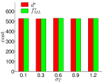
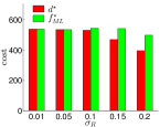
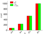
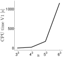
Verification 1	(a1)	(a2)	(a3)	(a4)
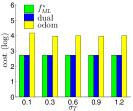
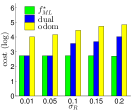
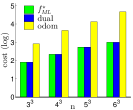
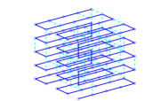
Primal via dual	(b1)	(b2)	(b3)	(b4)
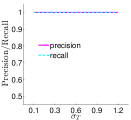
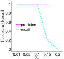
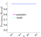
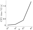
Verification 2	(c1)	(c2)	(c3)	(c4)

Figure 2: Statistics regarding the verification technique V1 (first row), the computation of the primal solution via the dual (second row), and the verification technique V2 (third row). Results are shown for different levels of translation noise $\sigma_{T}$ (first column), rotation noise $\sigma_{R}$ (second column), and size of the problem (third column). The rightmost column shows the CPU time required by V1 and V2 and the datasets used for the Monte Carlo simulations.

IV-B Primal Optimal Solutions

In this section, rather than verifying the quality of a given candidate solution, we show how to use duality to compute a primal optimal solution directly. We focus on the particular case in which the duality gap is zero. This case is of interest as we observe that the duality gap is often zero in practice.

From Lemma 1 we know that an optimal solution must be in the null space of ${\bm{M}}({\bm{\lambda}}^{\star})$. This motivates the following proposition, which provides a way to compute a primal optimal solution directly from the solution ${\bm{\lambda}}^{\star}$ of (54).

Proposition 5

If the duality gap is zero and ${\bm{\lambda}}^{\star}$ is an optimal solution of (54), then an optimal solution ${\bm{x}}^{\star}$ of (III-A) can be computed by solving the following linear system:

$$\left[\begin{array}[]{c}{\bm{H}}({\bm{\lambda}}^{\star})\\ {\bm{b}}^{\mathsf{T}}{\bm{A}}\end{array}\right]{\bm{x}}^{\star}=\left[\begin{array}[]{c}{\bm{A}}^{\mathsf{T}}{\bm{b}}\\ \lambda_{y}^{\star}-{\bm{b}}^{\mathsf{T}}{\bm{b}}\end{array}\right]\quad\text{(to be solved w.r.t. ${\bm{x}}^{\star}$)}$$ (56)

Proof:

From Lemma 1, we know that when the duality gap is zero, it holds ${\bm{M}}({\bm{\lambda}}^{\star})[{\bm{x}}^{\star}\;1]={\mathbf{0}}$. Then, recalling the structure of ${\bm{M}}({\bm{\lambda}}^{\star})$ from (III-B), it’s easy to see that (56) only rewrites the condition ${\bm{M}}({\bm{\lambda}}^{\star})[{\bm{x}}^{\star}\;1]={\mathbf{0}}$, moving the constant terms to the right-hand side. ∎

Note that Lemma 1 ensures that the linear system (56) admits a solution. Proposition 5 allows finding an optimal solution to the primal problem (III-A). If this satisfies the determinant constraints in (6), it follows that this solution is also optimal for the original PGO problem (6). While currently we cannot prove that the determinant constraints are always satisfied, this was always the case in our experiments.

V Experiments

In this section we show that the first verification technique in Proposition 4 (referred to as V1) enables accurate quantification of the sub-optimality gap of a candidate SLAM solution, but that current SDP solvers do not scale well with increasing problem size. The second verification technique in Proposition 4 (referred to as V2) provides a convenient alternative for large-scale problems: it is reliable and less computationally demanding. Finally, we provide empirical evidence that when the duality gap is zero we can compute an optimal solution from the solution of the dual problem, as suggested by Proposition 5. The SDP (54) is solved using SDPA [21].

Effectiveness of V1. Proposition 4(V1) ensures that for any candidate solution $\hat{{\bm{x}}}$, $f_{\tt ML}(\hat{{\bm{x}}})-d^{\star}$ represents an upper-bound on the sub-optimality gap $f_{\tt ML}(\hat{{\bm{x}}})-f_{\tt ML}^{\star}$ of $\hat{{\bm{x}}}$. However, it is possible that this bound is very loose, in which case it would be of little practical utility. In this section, we show that $d^{\star}$ is close to $f_{\tt ML}^{\star}$ in practice, hence $f_{\tt ML}(\hat{{\bm{x}}})-d^{\star}$ is a very good measure of the sub-optimality gap of the candidate $\hat{{\bm{x}}}$.

In our experiments we compute the “optimal” solution $f_{\tt ML}^{\star}$ of (6) by refining the chordal initialization of [22, 23] with 10 Gauss-Newton (GN) iterations. While one cannot guarantee a priori that this approach always produces the optimal estimate, using the results of this paper we will be able to check optimality a posteriori.

We evaluated how close $d^{\star}$ is to $f_{\tt ML}^{\star}$ on the cube dataset of Fig. 2(b4). In this dataset, the odometric trajectory is simulated as the robot travels on a 3D grid world, and random loop closures are added between nearby nodes, with probability $0.3$. Relative pose measurements are obtained by contaminating the true relative poses with zero-mean Gaussian noise, with standard deviation $\sigma_{T}$ and $\sigma_{R}$ for the translational and rotational noise, respectively. Statistics are computed over 10 runs: for each run we create a cube with random connectivity and random measurement noise. We consider an example with $n=5^{3}$ poses and varying noise levels $\sigma_{T}$ and $\sigma_{R}$.

Fig. 2(a1) shows $d^{\star}$ and $f_{\tt ML}^{\star}$ for different translational noise levels, fixing $\sigma_{R}=0.05\mbox{rad}$. The figure shows that $d^{\star}=f_{\tt ML}^{\star}$ (zero duality gap) independently on the translational noise level, hence $d^{\star}$ is a very good proxy of $f_{\tt ML}^{\star}$.

Fig. 2(a2) shows $d^{\star}$ and $f_{\tt ML}^{\star}$ for different rotational noise, fixing $\sigma_{T}=0.1\mbox{m}$. In this case the duality gap $f_{\tt ML}^{\star}-d^{\star}$ is more sensitive to the noise level, and for large rotational noise $d^{\star}$ becomes smaller than $f_{\tt ML}^{\star}$. However, the gap $f_{\tt ML}^{\star}-d^{\star}$ remains small, and is within $20\%$ of $f_{\tt ML}^{\star}$ in all cases.

Fig. 2(a3) shows $d^{\star}$ and $f_{\tt ML}^{\star}$ for different sizes of the cube dataset, fixing $\sigma_{R}=0.05\mbox{rad}$ and $\sigma_{T}=0.1\mbox{m}$. Again in this case $d^{\star}=f_{\tt ML}^{\star}$ (zero duality gap) independently of the size of the dataset. However, we observe that the SDP (54) becomes intractable for larger problem sizes, as shown in Fig. 2(a4).

Primal optimal solution via the dual. Here we demonstrate experimentally that one can recover a primal optimal solution ${\bm{x}}^{\star}$ for the SLAM problem from the dual optimal solution ${\bm{\lambda}}^{\star}$ of (54) whenever strong duality holds.

For each of the experimental trials described previously, we also computed an estimate $\hat{{\bm{x}}}$ for the SLAM solution directly from the optimal solution ${\bm{\lambda}}^{\star}$ for the dual program (54) using equation (56). Figs. 2(b1)-(b3) compare the value $f(\hat{{\bm{x}}})$ of this estimate against the value $f_{\tt ML}^{\star}$ of the solution obtained by solving the SLAM problem directly using the chordal initialization, and against the cost of the odometric guess.

We can see that for those experimental conditions in which strong duality holds (those experiments in Figs. 2(a1)-(a3) for which the green and red bars are the same height), the estimate $\hat{{\bm{x}}}$ in fact achieves the (certified) globally optimal cost $f_{\tt ML}^{\star}$ and is therefore a globally optimal solution for the SLAM problem, as guaranteed by Proposition 5. More interestingly, we also find that even in those cases when strong duality does not hold (in which case Proposition 5 no longer guarantees that $\hat{{\bm{x}}}$ is a primal optimal solution), the quality of the candidate $\hat{{\bm{x}}}$ degrades gracefully (i.e. the gap $f(\hat{{\bm{x}}})-f_{\tt ML}^{\star}$ increases gradually) with increasing noise levels. In particular, we find that $\hat{{\bm{x}}}$ outperforms the odometric guess in all tested cases.

These experiments confirm that we can extract a primal optimal solution ${\bm{x}}^{\star}$ for the SLAM problem directly from the solution ${\bm{\lambda}}^{\star}$ of the convex dual problem whenever strong duality holds. However, this approach is unfortunately not currently practical as a general-purpose SLAM technique, due to the high computational cost of solving large scale SDPs.

Effectiveness of V2. In this section we show that V2 is a computationally tractable verification approach, and it preserves the desirable properties of V1, i.e., it is able to discern optimal estimates from suboptimal ones. In contrast to V1, V2 does not quantify the sub-optimality gap, but can only give a binary answer: either it certifies that the estimate $\hat{{\bm{x}}}$ is optimal (by producing a dual certificate $\hat{{\bm{\lambda}}}$), or it is inconclusive. Before moving to the real tests, we consider the cube scenario discussed in the previous section.

We perform the following test: for each realization of the cube scenario, we compute the optimal solution ${\bm{x}}^{\star}$ (attaining $f_{\tt ML}^{\star}$) as in the previous tests, and a sub-optimal solution ${\bm{x}}^{\dagger}$ (attaining $f^{\dagger}>f^{\star}$) by bootstrapping the Gauss-Newton method with a random initial guess. Then, we apply the verification technique to both ${\bm{x}}^{\star}$ and ${\bm{x}}^{\dagger}$ and see if they pass the optimality test. Using the results we can compute the precision and recall of our classification:

$$\text{precision}=\frac{|{\color[rgb]{0,1,0}\checkmark}\;{\bm{x}}^{\star}|}{|{\color[rgb]{0,1,0}\checkmark}\;{\bm{x}}^{\star}|+|{\color[rgb]{0,1,0}\checkmark}\;{\bm{x}}^{\dagger}|}\;\;\text{recall}=\frac{|{\color[rgb]{0,1,0}\checkmark}\;{\bm{x}}^{\star}|}{|{\color[rgb]{0,1,0}\checkmark}\;{\bm{x}}^{\star}|+|{\color[rgb]{1,0,0}\mbox{X}}\;{\bm{x}}^{\star}|}$$ (57)

where $|{\color[rgb]{0,1,0}\checkmark}\;{\bm{x}}^{\star}|$ denotes the number of tests in which an optimal solution ${\bm{x}}^{\star}$ was accepted as optimal by V2, $|{\color[rgb]{0,1,0}\checkmark}\;{\bm{x}}^{\dagger}|$ is the number of tests in which a suboptimal solution was accepted as optimal, and $|{\color[rgb]{1,0,0}\mbox{X}}\;{\bm{x}}^{\star}|$ is the number of tests in which V2 was not able to certify the optimality of an optimal solution.

We point out that Proposition 4(V2) guarantees that our certification approach always has precision equal to $1$; however, recall may be less than $1$, and will be for cases in which strong duality does not hold. We plot precision/recall for different levels of translational and rotational noise, and for different sizes of the dataset, as shown in Figs. 2(c1)-(c2)-(c3). We observe that only for larger rotational noise Fig. 2(c2) the recall decreases; these are exactly the cases in which the duality gap is nonzero. (For $\sigma_{R}=0.2\mbox{rad}$, V2 was not able to certify optimality in any case, which means that the precision becomes undefined ($\frac{0}{0}$) and for this reason we do not show the corresponding data point in Fig. 2(c2).) Finally, Fig. 2(d2) shows the CPU time required by V2. This is the time required to solve the linear system (55), and check if ${\bm{M}}(\hat{{\bm{\lambda}}})\succeq 0$. V2 is computationally cheap, as it does not require solving the SDP.

We conclude the experimental part of this paper by testing the performance of the verification technique V2 on large-scale SLAM datasets. We consider the same datasets as [22]: the sphere, sphere-a, torus and cube are simulated datasets, while the garage, cubicle and rim are real datasets. For the results in this paper we substituted the covariances in the datasets of the scenarios sphere, sphere-a, garage, cubicle and rim with isotropic ones, as required by the PGO formulation (6).

Table I shows the results of the application of V2 to the SLAM datasets. The first column shows the cost obtained by applying a GN method starting from the initialization [22] (rows “Init.” in the table) and from the odometric guess (rows “Odom.”). These are the candidate solutions that we want to check, using V2. The columns “$d(\hat{{\bm{\lambda}}})$” and “$\mu$” show intermediate results of V2. In particular, $d(\hat{{\bm{\lambda}}})$ is the same one described in Proposition 4(V2), while $\mu$ is the smallest eigenvalue of ${\bm{M}}(\hat{{\bm{\lambda}}})$. Recall that V2 certifies optimality when $f_{\tt ML}(\hat{{\bm{x}}})=d(\hat{{\bm{\lambda}}})$ and $\mu\geq 0$ (if the smallest eigenvalue is non-negative, then ${\bm{M}}(\hat{{\bm{\lambda}}})\succeq 0$). We specify a tolerance in these tests, since the GN estimate $\hat{{\bm{x}}}$ will not attain the optimal solution ${{\bm{x}}}^{\star}$ exactly. Consequently, the solution $\hat{{\bm{\lambda}}}$ of (55) is not exact, so we consider that $f_{\tt ML}(\hat{{\bm{x}}})=d(\hat{{\bm{\lambda}}})$ if $|f_{\tt ML}(\hat{{\bm{x}}})-d(\hat{{\bm{\lambda}}})|/f_{\tt ML}(\hat{{\bm{x}}})<20\%$. Similarly, we add some tolerance to the condition $\mu\!\geq\!0$, and accept $\mu\!\!\geq\!\!-1$. Recall that $\mu$ is expected to be slightly negative, as the objective in (54) tends to push ${\bm{M}}({\bm{\lambda}})$ towards the boundary of the positive definite cone, and the SDP is solved numerically.

		$f_{\tt ML}(\hat{\bm{x}})$	$d(\hat{{\bm{\lambda}}})$	$\mu$	Time	V2
​​sphere	Init.	$5.7595\!\cdot\!10^{2}\!$	$5.75\!\cdot\!10^{2}\!$	$-1.80\!\cdot\!10^{-4}\!$	$609$	✓
$\begin{subarray}{c}n=2500\\ m=4949\end{subarray}$	Odom.	$5.8019\!\cdot\!10^{2}\!$	$4.38\!\cdot\!10^{2}\!$	$-1.45\!\cdot\!10^{-4}\!$	$597$	X
​​sphere-a	Init.	$1.2485\!\cdot\!10^{6}\!$	$1.25\!\cdot\!10^{6}\!$	$-9.64\!\cdot\!10^{-3}\!$	$332$	✓
$\begin{subarray}{c}n=2200\\ m=8647\end{subarray}$	Odom.	$3.0413\!\cdot\!10^{6}\!$	$3.04\!\cdot\!10^{6}\!$	$-1.01\!\cdot\!10^{2}\!$	$2.5$	X
​​torus	Init.	$1.2114\!\cdot\!10^{4}\!$	$1.21\!\cdot\!10^{4}\!$	$-7.85\!\cdot\!10^{-2}\!$	$39$	✓
$\begin{subarray}{c}n=5000\\ m=9048\end{subarray}$	Odom.	$2.7666\!\cdot\!10^{4}\!$	$2.76\!\cdot\!10^{4}\!$	$-1.04\!\cdot\!10^{2}\!$	$3.7$	X
​​cube	Init.	$4.216\!\cdot\!10^{4}\!$	$4.22\!\cdot\!10^{4}\!$	$-1.24\!\cdot\!10^{-2}\!$	$1646$	✓
$\begin{subarray}{c}n=8000\\ m=22236\end{subarray}$	Odom.	$2.7465\!\cdot\!10^{5}\!$	$2.74\!\cdot\!10^{5}\!$	$-9.98\!\cdot\!10^{1}\!$	$68.2$	X
​​garage	Init.	$\!\!6.2994\!\cdot\!10^{-1}\!$	$6.11\!\cdot\!10^{-1}\!$	$-6.78\!\cdot\!10^{-2}\!$	$12.3$	✓
$\begin{subarray}{c}n=1661\\ m=6275\end{subarray}$	Odom.	$\!\!6.2997\!\cdot\!10^{-1}\!$	$3.53\!\cdot\!10^{-1}\!$	$-6.75\!\cdot\!10^{-2}\!$	$11.2$	X
​​cubicle	Init.	$\!\!6.2481\!\!\cdot\!10^{2}\!\!$	$6.25\!\cdot\!10^{2}\!$	$-4.76\!\cdot\!10^{-1}\!$	$16.8$	✓
$\begin{subarray}{c}n=5750\\ m=16869\end{subarray}$	Odom.	$6.2484\!\cdot\!10^{2}\!$	$6.16\!\cdot\!10^{2}\!$	$-4.75\!\cdot\!10^{-1}\!$	$15.5$	✓
​​rim	Init.	$1.235\!\cdot\!10^{4}\!$	$1.23\!\cdot\!10^{4}\!$	$-9.77\!\cdot\!10^{1}\!$	$7.7$	X
$\begin{subarray}{c}n=10195\\ m=29743\end{subarray}$	Odom.	$1.6985\!\cdot\!10^{4}\!$	$-2.8\!\cdot\!10^{4}\!$	$-9.38\!\cdot\!10^{1}\!$	$7.1$	X

TABLE I: Verification technique V2 on large-scale SLAM datasets.

Let us start our analysis from the sphere dataset. When using the initialization (“Init.” row), the GN method attains an objective $5.7595\!\cdot\!10^{2}\!$. In this case, the two conditions for V2 are satisfied and we can certify the optimality of the resulting estimate (green check-mark in the rightmost column). When using the odometric initialization the resulting cost is larger (red entry in the column $f_{\tt ML}(\hat{\bm{x}})$), hence the estimate is suboptimal. V2 is able to identify the suboptimality, since $d(\hat{{\bm{\lambda}}})$ becomes much smaller than $f_{\tt ML}(\hat{\bm{x}})$. Hence V2 correctly decides not to certify the optimality of the odometric estimate (red “X” in the last column). Similar considerations hold for the second scenario, the challenging sphere-a: in this case the initialized estimate (shown in Fig. 1, top left) is accepted as optimal. The odometric estimate, instead, is trapped in a local minimum (Fig. 1, bottom left), and the optimality test V2 correctly rejects the estimate since it leads to a very negative $\mu$. Similar considerations hold for the torus, cube, and the cubicle datasets: our technique is able to discern optimal solutions from suboptimal estimates in all cases.

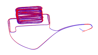
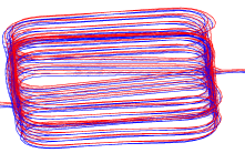
Figure 4: garage dataset: while the estimates obtained from GN with initialization (blue) and GN from odometry (red) attain a very similar cost ($6.2994\!\cdot\!10^{-1}\!$ versus $6.2997\!\cdot\!10^{-1}\!$), the corresponding trajectories are still different, which indicates that GN from odometry did not completely converge after 10 iterations.

For the garage dataset, the initialized estimate is classified as optimal, while the odometric estimate, which has a similar cost ($6.2997\!\cdot\!10^{-1}\!$ vs $6.2994\!\cdot\!10^{-1}\!\,$), is rejected as suboptimal. We observed the corresponding trajectory estimates (see Fig.4) and, while they are are both visually correct and have very similar costs, they do not overlap. This may indicate the presence of regions in the cost functions that are nearly flat, i.e., for which different estimates can have similar cost. Allowing for extra GN iterations, the odometric estimate converges to the same cost as the initialized one, and our technique is able to certify its optimality. Empirically, we observed that estimates that are suboptimal because they need extra iterations to converge tend to fail the check on $d(\hat{{\bm{\lambda}}})$ (compare with sphere and garage), while estimates that converge to a wrong minimum tend to fail the check on $\mu$ (compare with sphere-a, torus, and cube).

For the rim dataset, both estimates (“init” and “odom”) are rejected by V2. While the initialized estimate is visually correct, currently, we cannot conclude anything as it might be that there exists a better estimate (i.e., GN failed), or our technique failed because the duality gap was nonzero.

Finally, in the column “Time”, we report the CPU time (in seconds) required to perform the second verification technique. Most of the time here is spent computing the smallest eigenvalue $\mu$ of ${\bm{M}}(\hat{{\bm{\lambda}}})$, which was obtained using Matlab’s ${\tt eigs}$, specifying $-100$ as guess for the eigenvalue. The CPU time depends on the size of the problem, but also depends on the distance between our guess ($-100$) and the closest eigenvalue. We leave a more thorough investigation of these computational aspects for future work.

VI Conclusion

We show that Lagrangian duality is an effective tool to assess the quality of a given SLAM estimate. We propose two techniques to judge if an estimate is globally optimal (i.e., it is the ML estimate), and we show that when the duality gap is zero one can compute an optimal SLAM solution from the dual problem. The performance of our verification techniques is extensively tested in real and simulated datasets, including large-scale benchmarks. Many theoretical questions remain open, e.g., under which conditions the duality gap is zero? is it possible to derive bounds on the duality gap? We also leave as future work more practical problems, such as the one of exploring more efficient solvers for large SDPs, possibly exploiting problem structure.

-A Extended Proof of Lemma 1

Appendix A Extended Proof of Lemma 1

Here we give an alternative proof of Lemma 1. For the sake of readability, we restate the Lemma before proving it.

Lemma 6 (Primal optimal solution and zero duality gap)

If the duality gap is zero ($d^{\star}=f^{\star}$), then any primal optimal solution $[{\bm{x}}^{\star}\;1]$ of (III-A) is in the null space of the matrix ${\bm{M}}({\bm{\lambda}}^{\star})$, where ${\bm{\lambda}}^{\star}$ is the solution of the dual problem (54).

Proof:

Assume that the duality gap between the primal problem (III-A) and the dual problem (54) is zero:

$$d^{\star}=f^{\star}\Leftrightarrow\sum_{\begin{subarray}{c}i=1,\ldots,n-1\\ u=1,2,3\end{subarray}}\lambda^{\star}_{iuu}+\lambda_{y}^{\star}=\left\|{\bm{A}}{\bm{x}}^{\star}-{\bm{b}}y^{\star}\right\|^{2}$$ (58)

Now, since $[{\bm{x}}^{\star}\;y^{\star}]$ is a solution of the primal problem, it must also be feasible, hence the following equality holds:

$$\sum_{i=1}^{n-1}\bigg{[}\displaystyle\sum_{\begin{subarray}{c}u=1,2,3\end{subarray}}\lambda^{\star}_{iuu}(1-({\bm{x}}^{\star})^{\mathsf{T}}{{\bm{E}}}_{iuv}({\bm{x}}^{\star}))$$ (59)

$$+\!\!\!\!\displaystyle\sum_{\begin{subarray}{c}u,v=1,2,3\\ u\neq v\end{subarray}}\lambda^{\star}_{iuv}(-({\bm{x}}^{\star})^{\mathsf{T}}{{\bm{E}}}_{iuv}({\bm{x}}^{\star}))\bigg{]}+\lambda_{y}^{\star}(1-(y^{\star})^{2})=0$$

Therefore, we can subtract the left-hand side of (59) to the left-hand side of (58) without altering the result:

$$-\sum_{i=1}^{n-1}\bigg{[}\displaystyle\sum_{\begin{subarray}{c}u=1,2,3\end{subarray}}\lambda^{\star}_{iuu}(1-({\bm{x}}^{\star})^{\mathsf{T}}{{\bm{E}}}_{iuv}({\bm{x}}^{\star}))$$

$$-\!\!\!\!\displaystyle\sum_{\begin{subarray}{c}u,v=1,2,3\\ u\neq v\end{subarray}}\lambda^{\star}_{iuv}(-({\bm{x}}^{\star})^{\mathsf{T}}{{\bm{E}}}_{iuv}({\bm{x}}^{\star}))\bigg{]}-\lambda_{y}^{\star}(1-(y^{\star})^{2})$$

$$+\sum_{\begin{subarray}{c}i=1,\ldots,n\\ u=1,2,3\end{subarray}}\lambda^{\star}_{iuu}+\lambda_{y}^{\star}=\left\|{\bm{A}}{\bm{x}}^{\star}-{\bm{b}}y^{\star}\right\|^{2}$$ (60)

Noting that some terms in $\lambda^{\star}_{iuu}$ and $\lambda_{y}^{\star}$ cancel out, we get:

$$\sum_{i=1}^{n-1} \!\!\!\!\bigg{[}\displaystyle\sum_{\begin{subarray}{c}u=1,2,3\end{subarray}}\!\!\lambda^{\star}_{iuu}({\bm{x}}^{\star})^{\mathsf{T}}{{\bm{E}}}_{iuv}({\bm{x}}^{\star})+\!\!\!\!\displaystyle\sum_{\begin{subarray}{c}u,v=1,2,3\\ u\neq v\end{subarray}}\!\!\lambda^{\star}_{iuv}({\bm{x}}^{\star})^{\mathsf{T}}{{\bm{E}}}_{iuv}({\bm{x}}^{\star})\bigg{]}$$

$$+\lambda_{y}^{\star}(y^{\star})^{2}=\left\|{\bm{A}}{\bm{x}}^{\star}-{\bm{b}}y^{\star}\right\|^{2}$$

Reorganizing the terms as done in (III-B), we obtain:

$$\left[\begin{array}[]{c}{\bm{x}}^{\star}\\ y^{\star}\end{array}\right]^{\mathsf{T}}\left[\begin{array}[]{cc}{\bm{H}}({\bm{\lambda}}^{\star})&-{\bm{A}}^{\mathsf{T}}{\bm{b}}\\ -{\bm{b}}^{\mathsf{T}}{\bm{A}}&{\bm{b}}^{\mathsf{T}}{\bm{b}}-\lambda_{y}^{\star}\end{array}\right]\left[\begin{array}[]{c}{\bm{x}}^{\star}\\ y^{\star}\end{array}\right]=0$$ (67)

which implies that $[{\bm{x}}^{\star}\;y^{\star}]$ is the null space of ${\bm{M}}({\bm{\lambda}}^{\star})$, proving the claim. ∎

A-A Estimated Trajectories for the Datasets in Table I

	GN from initialization	GN from odometry
sphere
sphere-a
torus

cube
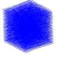
garage
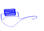
cubicle
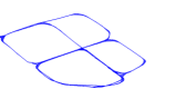
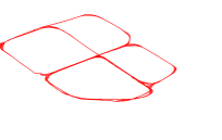
rim

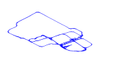
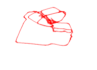
Figure 3: Blue: Estimated trajectory obtained by refining the chordal initialization of [22] with 10 Gauss-Newton iterations. Red: Estimated trajectory obtained by refining the odometric guess with 10 Gauss-Newton iterations.

garage: zoomed-in view and comparison

References

- [1] F. Lu and E. Milios, “Globally consistent range scan alignment for environment mapping,” Autonomous Robots, pp. 333–349, Apr 1997.
- [2] R. Kümmerle, G. Grisetti, H. Strasdat, K. Konolige, and W. Burgard, “g2o: A general framework for graph optimization,” in Proc. of the IEEE Int. Conf. on Robotics and Automation (ICRA), Shanghai, China, May 2011.
- [3] M. Kaess, H. Johannsson, R. Roberts, V. Ila, J. Leonard, and F. Dellaert, “iSAM2: Incremental smoothing and mapping using the Bayes tree,” Intl. J. of Robotics Research, vol. 31, pp. 217–236, Feb 2012.
- [4] E. Olson, J. Leonard, and S. Teller, “Fast iterative alignment of pose graphs with poor initial estimates,” in IEEE Intl. Conf. on Robotics and Automation (ICRA), May 2006, pp. 2262–2269.
- [5] G. Grisetti, C. Stachniss, and W. Burgard, “Non-linear constraint network optimization for efficient map learning,” Trans. on Intelligent Transportation systems, vol. 10, no. 3, pp. 428–439, 2009.
- [6] D. Rosen, M. Kaess, and J. Leonard, “RISE: An incremental trust-region method for robust online sparse least-squares estimation,” IEEE Trans. Robotics, 2014.
- [7] F. Dellaert and A. Stroupe, “Linear 2D localization and mapping for single and multiple robots,” in IEEE Intl. Conf. on Robotics and Automation (ICRA), May 2002.
- [8] L. Carlone, R. Aragues, J. Castellanos, and B. Bona, “A fast and accurate approximation for planar pose graph optimization,” Intl. J. of Robotics Research, 2014.
- [9] L. Carlone and F. Dellaert, “Duality-based verification techniques for 2D SLAM,” in Intl. Conf. on Robotics and Automation (ICRA), accepted, 2015.
- [10] D. Rosen and J. Leonard, “A convex relaxation for approximate global optimization in simultaneous localization and mapping,” in IEEE Intl. Conf. on Robotics and Automation (ICRA), 2015.
- [11] R. Tron, B. Afsari, and R. Vidal, “Intrinsic consensus on SO(3) with almost global convergence,” in IEEE Conf. on Decision and Control, 2012.
- [12] L. Carlone and A. Censi, “From angular manifolds to the integer lattice: Guaranteed orientation estimation with application to pose graph optimization,” IEEE Trans. Robotics, 2014.
- [13] S. Huang, Y. Lai, U. Frese, and G. Dissanayake, “How far is SLAM from a linear least squares problem?” in IEEE/RSJ Intl. Conf. on Intelligent Robots and Systems (IROS), 2010, pp. 3011–3016.
- [14] H. Wang, G. Hu, S. Huang, and G. Dissanayake, “On the structure of nonlinearities in pose graph SLAM,” in Robotics: Science and Systems (RSS), 2012.
- [15] L. Carlone, “Convergence analysis of pose graph optimization via Gauss-Newton methods,” in IEEE Intl. Conf. on Robotics and Automation (ICRA), 2013, pp. 965–972.
- [16] K. Khosoussi, S. Huang, and G. Dissanayake, “Novel insights into the impact of graph structure on SLAM,” in IEEE/RSJ Intl. Conf. on Intelligent Robots and Systems (IROS), 2014.
- [17] N. Boumal, A. Singer, and P. Absil, “Cramer-rao bounds for synchronization of rotations,” Information and Inference, vol. 3, no. 1, pp. 1–39, 2014.
- [18] R. Hartley, J. Trumpf, Y. Dai, and H. Li, “Rotation averaging,” IJCV, vol. 103, no. 3, pp. 267–305, 2013.
- [19] S. Boyd and L. Vandenberghe, Convex optimization. Cambridge University Press, 2004.
- [20] G. Calafiore and L. E. Ghaoui, Optimization Models. Cambridge University Press, 2014.
- [21] M. Yamashita, K. Fujisawa, and M. Kojima, “Implementation and evaluation of SDPA 6.0 (semidefinite programming algorithm 6.0),” Optimization Methods and Software, vol. 18, no. 4, pp. 491–505, Aug. 2003.
- [22] L. Carlone, R. Tron, K. Daniilidis, and F. Dellaert, “Initialization techniques for 3D SLAM: a survey on rotation estimation and its use in pose graph optimization,” in IEEE Intl. Conf. on Robotics and Automation (ICRA), 2015.
- [23] D. Martinec and T. Pajdla, “Robust rotation and translation estimation in multiview reconstruction,” in IEEE Conf. on Computer Vision and Pattern Recognition (CVPR), 2007, pp. 1–8.