Constraints on neutrino masses coming from magnetic dipole moments in a two Higgs doublet model type I and II

Abstract

In the framework of a two Higgs doublet model type I and type II, we calculate limits on neutrino masses for the different types of neutrinos, by using the experimental bounds on their magnetic dipole moments. This is carried out by analyzing diagrams of Cherenkov neutrino decays with a charged Higgs into the loop, coming  from the two Higgs doublet model (2HDM). Such constraints are translated into allowed regions in the free parameters of the models, for each neutrino flavor.

The analysis was performed by sweeping the charged Higgs mass between $(100-900)GeV$ and taking into account the experimental constraints for $\tan\beta$ in the 2HDM type I and II, obtaining contributions close to the experimental thresholds for muon and tau neutrinos, while for electron neutrino the relevant contribution comes from standard model and keeps out of the reach of forthcoming experiments.

PACS: 41.20.Cv, 02.10.Yn, 01.40.Fk, 01.40.gb, 02.30.Tb

1 Introduction

The phenomenon of neutrino oscillations, has been supported by the discovery of flavor conversions of neutrinos from different sources, like the atmospheric neutrinos made by Super-Kamiokande in 1998[1], or more recently by T2K Collaboration[2]. These oscillations occur among at least three types of flavors of neutrinos: electron, muon and tau neutrinos.

$$\left|\nu_{\alpha}\right\rangle=\sum\limits_{k}U_{\alpha k}^{\ast}\left|\nu_{k}\right\rangle\text{ \ \ \ \ \ \ \ }\left(\alpha=e,~{}\mu,~{}\tau\right)$$ (1)

all neutrinos produced and observed so far, have left-handed helicities, while all antineutrinos have right-handed helicities. Neutrino oscillations provided the first glimpse of physics beyond the standard model of particles. Now, since neutrino oscillations are sensitive only to the difference in the squares of their masses, such a phenomenon requires that at least two neutrino species have nonzero mass. The transition probability between different flavors can be approximated by

$$P_{\nu_{\alpha}\rightarrow\nu_{\beta}}\left(t\right)=\sum\limits_{k,j}U_{\alpha k}^{\ast}U_{\beta k}U_{\alpha j}U_{\beta j}^{\ast}\exp\left(-i\frac{\Delta m_{kj}^{2}L}{2E}\right)$$ (2)

where $P_{\nu_{\alpha}\rightarrow\nu_{\beta}}\left(t\right)$ is the probability that after travelling a distance $L$, a neutrino with flavor $\nu_{\alpha}$ converts into a neutrino with flavor $\nu_{\beta}$. As for the neutrino masses, we have only upper bounds hitherto[3]

$$m_{\nu_{e}}\leq 2.05eV\ ,\ \ m_{\nu_{\mu}}\leq 0.19MeV\ ,\ \ m_{\nu_{\tau}}\leq 18.2MeV$$ (3)

All elementary fermions in the Standard Model are Dirac fermions. Nevertheless, the nature of the neutrino is not yet definitely settled and depending on the model the neutrino can be either a Majorana or Dirac fermion. On the other hand, despite the neutrinos do not carry electric charge, they can participate in electromagnetic interactions by coupling with photons via loop diagrams, and like other particles the electromagnetic properties can be described by electromagnetic form factors (EFF’s). For example, by means of its multipole moments, neutrinos can be sensitive to intense electromagnetic fields, and such intense fields can exist in nature. It has been suggested that there could be sources of magnetic fields of order $\left(10^{13}-10^{18}\right)G$, as it could be the case during a supernova explosion or in the vicinity of special groups of neutron stars known as magnetars[4].

On the other hand, present limits on the scalar sector in the standard model, still permits the possibility of an extended Higgs sector. We shall study one of the simplest extension of the scalar sector of the standard model, the so-called Two Higgs Doublet Model (2HDM) in which we add a second Higgs doublet with the same quantum numbers of the first. There are many motivations for this model, one of this is the fact that the SM is unable to generate a baryon asymmetry of the universe of sufficient size, or to explain the mass hierarchy in the third generation of quarks. Two Higgs Doublet models are possible scenarios to solve these problems, due to the flexibility of their scalar mass spectrum and the existence of additional sources of $CP$ violation. In addition in the Minimal Supersymmetric Standard Model (MSSM), a second doublet should be added in order to cancel anomalies[5].

The coupling of neutrinos with photons occur via loop diagrams. In the Standard Model (SM), the loop corrections have the form of vertex diagrams and vacuum polarization diagrams. When a second doublet of scalars is included in the spectrum, further corrections appear by replacing the vector bosons $W^{\pm}$ by charged Higgs bosons $H^{\pm}$. Our goal is to characterize the corrections to the EFF’s coming from the new physics, and particularly on the region of parameters in which such factors become near the threshold of detection. In the region of parameters in which the threshold of detection is reached, we obtain bounds on neutrino masses.

The structure of this paper is as follows. In section 2 we discuss briefly the implementation of neutrino Dirac masses in SM. In section 3 we discuss the general form of the EFF’s for neutrinos. In section 4 we describe briefly the two Higgs doublet Model (2HDM), particularly the models of type I and of type II as well as the implementation of neutrinos masses into those models. In section 5, we characterize the loop diagrams coming from the 2HDM that contributes to the EFF’s of the neutrino. In section 6 we find upper bounds for the neutrino masses in the framework of the 2HDM type I and II, by using the allowed values of the free parameters of the model, as well as the experimental limits for the magnetic dipole moments of such neutrinos. Finally, section 7 yields our conclusions.

2 Neutrino Dirac mass term in SM

There are several ways to incorporate neutrino masses within the SM or its extensions, in order to explain the observed neutrino oscillations. We shall use a simple form which consists of adding right-handed singlets of neutrinos fields $\left(\nu_{\alpha^{\prime}R}\right)$ corresponding to each charged lepton. This insertion implies new gauge invariant interactions in the Yukawa sector

$$-\mathcal{L}_{Yukawa}=\sum\limits_{\alpha=e,\mu,\tau}\sum\limits_{\alpha^{\prime}=1}^{3}f_{\alpha,\alpha^{\prime}}\overline{\psi}_{\alpha L}\widetilde{\Phi}\nu_{\alpha^{\prime}R}+h.c$$ (4)

where $f_{\alpha,\alpha^{\prime}}$ is a matrix with new coupling constants, $\psi_{\alpha L}$ is the left-handed lepton doublet and $\Phi$ is the SM Higgs doublet, with $\widetilde{\Phi}\equiv i\sigma_{2}\Phi^{\ast}$

$$\left\langle\Phi\right\rangle=\frac{1}{\sqrt{2}}\left(\begin{array}[]{c}0\\ v\end{array}\right)$$ (5)

a nonzero vacuum expectation value (VEV) of the Higgs doublet induces the spontaneous symmetry breaking from $SU\left(2\right)_{L}\times U\left(1\right)_{Y}$ to $U\left(1\right)_{Q}$. In turn, the VEV also provides the neutrino Dirac mass term

$$-\mathcal{L}_{D_{mass}}=\frac{v}{\sqrt{2}}\sum\limits_{\alpha=e,\mu,\tau}\sum\limits_{\alpha^{\prime}=1}^{3}f_{\alpha,\alpha^{\prime}}\overline{\nu}_{\alpha L}\nu_{\alpha^{\prime}R}+h.c$$ (6)

In general the matrix $f_{\alpha,\alpha^{\prime}}$ is a complex $3\times 3$ matrix, the massive neutrino fields are obtained through the diagonalization of $\mathcal{L}_{D_{mass}}$ , this can be done by diagonalizing $f_{\alpha,\alpha^{\prime}}$ with a biunitary transformation

$$\frac{v}{\sqrt{2}}\left(U^{\dagger}~{}f~{}V\right)_{k,j}=m_{k}\delta_{kj}$$ (7)

where $m_{k}$ is a diagonal matrix with real and positive values.

The flavor eigenstates $\nu_{e},~{}\nu_{\mu}$ and $~{}\nu_{\tau}$ are superpositions of the mass eigenstates

$$\nu_{\alpha L}=\sum\limits_{k=1}^{3}U_{\alpha,k}\nu_{kL}\ \ ;\ \ \nu_{\alpha^{\prime}R}=\sum\limits_{j=1}^{3}V_{\alpha^{\prime},j}\nu_{jR}$$

or equivalently, the mass eigenstates $\nu_{k}$ are mixtures of flavor eigenstates. The mixing matrix $U$ is called the PMNS matrix due to Pontecorvo[6], Maki, Nakagawa and Sakata[7].

The result of the diagonalization gives Dirac mass terms of the form

$$-\mathcal{L}_{D_{mass}}=\sum\limits_{k=1}^{3}m_{k}\overline{\nu}_{k}\nu_{k}$$ (8)

with the Dirac fields of massive neutrinos given by

$$\nu_{k}=\nu_{kL}+\nu_{kR}$$ (9)

3 The electromagnetic form factors (EFF’s)

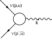
Figure 1: Effective coupling of two neutrinos with a photon

$$\left\langle u\left(p,\lambda\right)|J_{\mu}^{EM}\left(x\right)|u\left(p^{\prime},\lambda^{\prime}\right)\right\rangle=\overline{u}\left(p,\lambda\right)\Lambda_{\mu}\left(l,q\right)u\left(p^{\prime},\lambda^{\prime}\right)$$ (10)

To find all the EFF’s, we use the general expression for the current[8],[9], where $q_{\mu}=p_{\mu}^{\prime}-p_{\mu}$, $l_{\mu}=p_{\mu}^{\prime}+p_{\mu}$ are the four-momenta shown in Fig. 1, and $u\left(p,\lambda\right)$, $u\left(p^{\prime},\lambda^{\prime}\right)$ are the initial and final fermion states respectively. Further, $\Lambda_{\mu}$ are matrices of couplings acting on the spinors. The matrices $\Lambda_{\mu}$ have some interesting properties

• The first condition is that the arrangement $\Lambda_{\mu}$ must be a 4-vector, i.e. must be Lorentz covariant.

• The second condition is hermiticity of the associated current, i.e., $J_{\mu}^{{}^{{\dagger}}EM}=J_{\mu}^{EM}$ which implies

  $$\Lambda_{\mu}\left(l,q\right)=\gamma^{0}\Lambda_{\mu}^{{\dagger}}\left(l,-q\right)\gamma^{0}$$ (11)

• The current conservation or gauge invariance $\partial^{\mu}J_{\mu}^{EM}=0$ can be recast into

  $$q^{\mu}\overline{u}\left(p^{\prime},\lambda^{\prime}\right)\Lambda_{\mu}\left(l,q\right)u\left(p,\lambda\right)=0$$ (12)

The most general expression for $\Lambda_{\mu}\left(l,q\right)$ reads[10]

$$\Lambda_{\mu}\left(q\right) = F_{Q}\left(q^{2}\right)\gamma_{\mu}+\left[F_{M}\left(q^{2}\right)i+F_{E}\left(q^{2}\right)\gamma_{5}\right]\sigma_{\mu\nu}q^{\nu}+F_{A}\left(q^{2}\right)\left(q^{2}\gamma_{\mu}-q_{\mu}\not{q}\right)\gamma_{5}$$ (13)

where $F_{Q},~{}F_{M},~{}F_{E}$ and $F_{A}$ represent the electric charge, dipole magnetic moment, dipole electric moment and anapole moment respectively.

The EFF’s show us how the particles are coupled with the photon at the tree level or in loop corrections. At the tree level we got the electric charge and one part of the contribution coming from the magnetic dipole moment. Now, if we consider the interaction with an external field $A_{ext}^{\mu}$ in the form

$$\mathcal{L}_{ext}=-eA_{ext}^{\mu}J_{\mu}^{EM}$$ (14)

the so-called anomalous magnetic moment arises. Even uncharged particles may have magnetic dipole moment. However, for uncharged particles all dipole moments only appear in loop corrections. Just like the anomalous magnetic moment, the dipole electric moment and the anapole moment can be non-zero even for an uncharged particle[11]. We summarize some electromagnetic properties of charged leptons in table 1

$$l$$ Mass MDM EDM

Table 1: Electromagnetic properties of charged leptons, MDM represents the magnetic dipole moment and EDM electric dipole moment

Like other particles, neutrinos can be described by EFF’s with vertex functions. For neutrinos the magnetic and electric dipole moments are expected to be very small since they are likely proportional to the neutrino masses. For the anomalous magnetic moment the leading contribution is [11]

$$a_{\nu_{i}}=-\frac{3G_{F}m_{\nu_{i}}}{4\sqrt{2}\pi^{2}}m_{e}$$ (15)

Consequently, the neutrino magnetic moment is [15]

$$\vec{\mu}_{\nu_{i}} = -\frac{e}{m_{e}}a_{\nu_{i}}\vec{s}_{\nu_{i}}$$

$$\Rightarrow \mu_{\nu}=-\frac{3G_{F}em_{\nu_{i}}}{4\sqrt{2}\pi^{2}}\simeq 3.2\times 10^{-19}\left(\frac{m_{\nu}}{1eV}\right)\mu_{B}$$

where $\mu_{B}$ is the Bohr’s magneton. If neutrino couples to photons via such moments, the neutrino electromagnetic properties can be used to distinguish Majorana and Dirac neutrinos. For Dirac neutrinos the most relevant moment is $F_{M}$, because the other terms vanish in a $CP-$conserving scenario with an hermitian $J_{\mu}^{EM}$, and are highly supressed owing to the soft violation of $CP$. On the other hand, for Majorana neutrinos only $F_{A}$ is possible, because the other terms vanish owing to the self-conjugate nature of Majorana neutrinos. Table 2 summarizes the electromagnetic properties of massive neutrinos[11]

$$l$$ Mass Magnetic dipole moment

Table 2: Electromagnetic properties of massive neutrinos.

4 The two Higgs doublet model with massive neutrinos

The 2HDM contains five Higgs bosons in its spectrum[12]. The symmetry breaking is implemented by introducing a new scalar doublet with the same quantum numbers of the first one[13]. In a CP-conserving scenario, the Higgs sector consists of: Two Higgs CP-even scalars $\left(H^{0},h^{0}\right),$ one CP-odd scalar $\left(A^{0}\right)$ and two charged Higgs bosons $\left(H^{\pm}\right)$. A key parameter of the model is the ratio between the vacuum expectation values

$$\tan\beta=\frac{v_{2}}{v_{1}}$$ (17)

where $v_{1}$ and $v_{2}$ are the vacuum expectation values of the Higgs doublets[14], with values of $0\leq\beta\leq\frac{\pi}{2}$.

The most general gauge invariant Lagrangian that couples the Higgs fields to leptons (with massless neutrinos) reads

$$-\mathcal{L}_{Y}=\eta_{i,j}^{E,0}\overline{l}_{iL}^{0}\Phi_{1}E_{jR}^{0}+\xi_{i,j}^{E,0}\overline{l}_{iL}^{0}\Phi_{2}E_{jR}^{0}+h.c.$$

where $\Phi_{1,2}\;$represents the Higgs doublets, and$\ \widetilde{\Phi}_{1,2}\equiv i\sigma_{2}\Phi_{1,2}$, The superscript “$0$” indicates that the fields are not mass eigenstates yet,$\;\eta_{i,j}\;$and $\xi_{i,j}\;$are non diagonal $3\times 3$ matrices with $\left(i,j\right)\;$denoting family indices. $E_{jR}^{0}\;$denotes the three charged leptons and$\ \overline{l}_{iL}^{0}\;$denotes the lepton weak isospin left-handed doublets.

It is customary to implement a discrete symmetry in the 2HDM in order to suppress some processes such as the Flavor Changing neutral currents (FCNC). In particular by demanding the discrete symmetry

$$\Phi_{1} \rightarrow \Phi_{1}\ \ ;\ \ \ \Phi_{2}\rightarrow-\Phi_{2}$$

$$D_{jR} \rightarrow \mp D_{jR}\ \ ;\ \ U_{jR}\rightarrow-U_{jR}$$ (18)

such kind of processes are eliminated at the tree-level. Here $D_{jR}$ and$\ U_{jR}$ denote right-handed singlets of the down and up types of fermions.

4.1 The 2HDM type I

By taking $D_{jR}\rightarrow-D_{jR}$ we arrive to the so-called 2HDM of type I. In this scenario, only $\Phi_{2}\;$couples in the Yukawa sector and gives masses to all fermions. The Lepton Yukawa Lagrangian becomes

$$-\mathcal{L}_{Y}=\eta_{ij}^{E,0}\overline{l}_{iL}^{0}\widetilde{\Phi}_{2}\nu_{jR}^{0}+\xi_{ij}^{E,0}\overline{l}_{iL}^{0}\Phi_{2}E_{jR}^{0}+h.c.$$ (19)

and the term of charged current of the Lagrangian with leptons yields

$$-\mathcal{L}_{Y}=\frac{g\cot\beta}{\sqrt{2}M_{W}}\overline{l}\left(M_{l}^{diag}P_{R}-M_{\nu}^{diag}P_{L}\right)\nu H^{+}+h.c.$$ (20)

4.2 The 2HDM type II

If we use $D_{jR}\rightarrow D_{jR}\;$ we obtain the so-called 2HDM of type II. In this model $\Phi_{1}$ couples and gives masses to the down sector, while $\Phi_{2}$ couples and gives masses to the up sector. In consequence, the Lepton Yukawa Lagrangian (with massless neutrinos) becomes

$$-\mathcal{L}_{Y}=\eta_{ij}^{D,0}\overline{l}_{iL}^{0}\widetilde{\Phi}_{1}E_{jR}^{0}+\xi_{ij}^{\nu,0}\overline{l}_{iL}^{0}\Phi_{2}\nu_{jR}^{0}+h.c.$$ (21)

and the term of charged current of the lagrangian with leptons gives

$$\mathcal{L}_{Y}=\frac{g}{\sqrt{2}M_{W}}\overline{\nu}\left[\left(\cot\beta M_{\nu}^{diag}P_{L}+\tan\beta M_{l}^{diag}P_{R}\right)\right]lH^{+}+h.c.$$

An interesting aspect is that the limits for the parameter space ($m_{H^{+}},\tan\beta$), for model type II are very similar to those obtained by considering the minimal supersymmetric scenario.

4.3 2HDM type I and II with massive neutrinos

The term (4) inserted in the Yukawa sector of the standard model should also be inserted in the two Higgs doublet model for each doublet $\Phi_{i}$. Nevertheless, when we implement the discrete symmetry (18) in a Lagrangian of the form (4) we observe that the term involving the doublet $\Phi_{1}$ cannot appear, and that the extra term is the same in either model type I or model type II.

5 Radiative corrections in 2HDM

The diagrams that contribute to the neutrino electromagnetic vertex in SM are displayed in Fig. 2

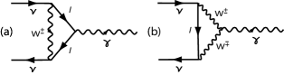
Figure 2: Loop corrections with leptons and $W^{\pm}$ vector bosons in SM.

And for the vacuum polarization they are shown in Fig. 3.

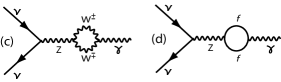
Figure 3: Vacuum polarization with $W^{\pm}$ vector bosons, and fermions denoted by $f$ in SM.

Within the framework of a 2HDM with massive neutrinos, we should add three new types of diagrams: two vertex corrections illustrated in Fig. 4, and one correction to the vacuum polarization displayed in Fig. 5. They arise by replacing $W^{\pm}$ by $H^{\pm}$ in the SM diagrams.

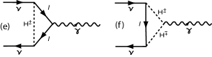
Figure 4: Loop corrections with leptons and $H^{\pm}$ in the 2HDM.

Figure 5: Vacuum polarization with $H^{\pm}$ in the 2HDM.

Fig. 4(f) shows the vertex correction involving two charged Higgs bosons and one charged lepton into the loop $\left(2H^{\pm}1L\right)$. For this diagram, the general form of the contribution can be written as

$$\Lambda_{2H^{\pm}1L}^{\alpha}\left(q,l\right)=-e\int\frac{d^{4}k}{\left(2\pi\right)^{4}}\left\{\frac{\left(2k^{\alpha}+p_{2}^{\alpha}+p_{1}^{\alpha}\right)\left(aP_{L}+bP_{R}\right)\left(\not{k}+m_{l}\right)\left(cP_{L}+dP_{R}\right)}{\left[\left(k+p_{1}\right)^{2}-m_{H^{\pm}}^{2}\right]\left[\left(k+p_{2}\right)^{2}-m_{H^{\pm}}^{2}\right]\left(k^{2}-m_{l}^{2}\right)}\right\}$$

where $a,b,c$ and $d$ are constants associated with the Feynman rules of the 2HDM, with $P_{R,L}=\left(1\pm\gamma^{5}\right)/2$. The contribution to the EFF’s of this diagram is described in the appendix, and in particular, the contribution to the magnetic dipole moment (MDM) is given by

$$\Lambda_{2H^{\pm}1L}^{\alpha}\left(q,l\right)_{MDM}=\frac{-ie}{16\pi^{2}}\int\limits_{0}^{1}dx\int\limits_{0}^{x}dy\frac{1}{P^{2}}\left[\left(m_{\nu}-\frac{1}{2}m_{l}\right)+\left(m_{l}-3m_{\nu}\right)x+2x^{2}m_{\nu}\right]i\sigma^{\alpha\mu}q_{\mu}\left[\left(ac+bd\right)+\left(bd-ac\right)\gamma_{5}\right]$$

On the other hand, the diagram in Fig. 4(e) with two leptons and one charged Higgs into the loop $\left(2L1H^{\pm}\right)$, gives a contribution of the form

$$\Lambda_{2L1H}^{\alpha}\left(q,l\right)=-e\int\frac{d^{4}k}{\left(2\pi\right)^{4}}\left\{\frac{\left(aP_{L}+bP_{R}\right)\left(\not{k}+\not{p}_{1}+m_{l}\right)\gamma^{\alpha}\left(\not{k}+\not{p}_{2}+m_{l}\right)\left(cP_{L}+dP_{R}\right)}{\left[\left(k+p_{1}\right)^{2}-m_{l}^{2}\right]\left[\left(k+p_{2}\right)^{2}-m_{l}^{2}\right]\left(k^{2}-m_{H^{\pm}}^{2}\right)}\right\}$$

from which we obtain the contribution of this diagram to the MDM, that is given by

$$\Lambda_{2L1H^{\pm}}^{\alpha}\left(q,l\right)_{MDM}=\frac{-ie}{16\pi^{2}}\int\limits_{0}^{1}dx\int\limits_{0}^{x}dy\frac{1}{P^{2}}\left(2x^{2}m_{\nu}+m_{l}x-xm_{\nu}\right)i\sigma^{\alpha\mu}q_{\mu}\left[\left(ac+bd\right)+\left(bd-ac\right)\gamma_{5}\right]$$

On the other hand the contribution of the vacuum polarization vanishes. Therefore, the full contribution to the MDM yields

$$\Lambda_{2HDM}^{\alpha}\left(q,l\right)_{MDM}=\Lambda_{2H^{\pm}1L}^{\alpha}\left(q,l\right)_{MDM}+\Lambda_{2L1H^{\pm}}^{\alpha}\left(q,l\right)_{MDM}$$ (22)

for the 2HDM type I, the values of $a,b,c$ and $d$ are

$$a=c=\frac{2^{\frac{3}{4}}\sqrt{G_{F}}}{\tan\beta}m_{v_{l}}\ \ ;\ \ b=d=\frac{2^{\frac{3}{4}}\sqrt{G_{F}}}{\tan\beta}m_{l}$$

we shall use the numerical value

$$G_{F}=\frac{\sqrt{2}}{8}\frac{g^{2}}{M_{W}^{2}}=1.1663787(6)\times 10^{-5}GeV^{-2}$$

as for the 2HDM type II, the values of $a,b,c$ and $d$ are given by

$$a=c=\frac{2^{\frac{3}{4}}\sqrt{G_{F}}}{\tan\beta}m_{v_{l}}\ ;\ \ b,d=2^{\frac{3}{4}}\sqrt{G_{F}}m_{l}\tan\beta$$

6 Results and analysis

Our analysis will be based on constraints on charged Higgs masses and the $\tan\beta$ parameter. For either model type I or II the experimental constraints on the possible values in the $\left(m_{H^{\pm}},\tan\beta\right)$ parameter space comes from processes such as $B_{u}\rightarrow\tau\nu_{\tau},~{}D_{s}\rightarrow\tau\nu_{\tau},~{}B\rightarrow D\tau\nu_{\tau},~{}K\rightarrow\mu\nu_{\mu}$ and $BR\left(B\rightarrow X_{s}\gamma\right)$[16].

Based on the phenomenological constraints on the 2HDM type I, we take values of $\tan\beta$ between $\left(2-90\right)$ and values of the charged Higgs mass of $m_{H^{\pm}}=\left(100-300-500-700-900\right)GeV\$[17]. On the other hand, for the 2HDM type II, we have different allowed intervals of $\tan\beta$ for different values of the charged Higgs mass: for $m_{H^{\pm}}=300GeV$ the values of $\tan\beta$ lie within the interval $\left(4-40\right)$, for $m_{H^{\pm}}=500GeV$ the value of $\tan\beta$ is between $\left(2-69\right)$ and for $m_{H^{\pm}}\left(700-900\right)GeV$ the values of $\tan\beta$ is between $\left(1-70\right)\$[17].

We shall make contourplots of the neutrino mass versus MDM of the neutrino for different values of the charged Higgs mass sweeping all allowed values of $\tan\beta$ for each mass. As for the neutrino masses, we shall plot up to an order of magnitude higher than the upper bound of the SM.

• Electron neutrino case

Taking into account the upper experimental bound in the SM for the electron neutrino mass$\ m_{\nu_{e}}$, we shall plot within the interval $1\times 10^{-8}MeV\leq m_{\nu_{e}}\leq 1\times 10^{-5}MeV$. If we use the above interval in a model with two Higgs doublets, for different values of Higgs mass and $\tan\beta$, we shall obtain exclusion regions by taking as reference the experimental thresholds for the MDM of the electron neutrino. In this way, it is possible to obtain upper bounds on the neutrino mass in this scenario.

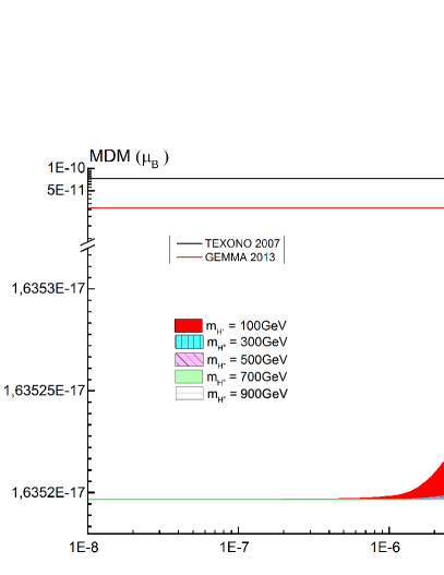
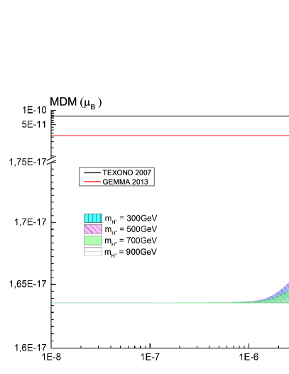
Figure 6: The graphics show the values of the magnetic dipole moment (MDM) as a function of the electron neutrino mass between $\left(1\times 10^{-8}-1\times 10^{-5}\right)MeV$ and for values of the charged Higgs mass of $\left(100-300-500-700-900\right)GeV$ for the 2HDM type I (left-hand side) and $\left(300-500-700-900\right)GeV$ for the 2HDM type II (right-hand side).

In Fig. 6, we plot the electron neutrino mass versus MDM for charged Higgs masses of $100,\ 300,\ 500,\ 700,900\ GeV$ for the 2HDM type I (left-hand side) and for masses of $300,500,700,900$ $GeV$ for the 2HDM type II (right-hand side). The horizontal lines correspond to the experimental upper limits for MDM coming from TEXONO 2007 (Taiwan EXperiment On NeutriNO) [18] which is $\mu_{\overline{\nu}_{e}}<7.4\times 10^{-11}\mu_{B}$ at $90\%~{}C.L.$, and GEMMA 2013. (Germanium Experiment for measurement of Magnetic Moment of Antineutrino)[19] which is $\mu_{\nu_{e}}<2.9\times 10^{-11}\mu_{B}$ at $90\%~{}C.L.$. We observe that the maximum values of MDM that can be reached are $1.635\times 10^{-17}\mu_{B}$ for a value of the charged Higgs mass of $m_{H^{\pm}}=100GeV$ and $\tan\beta=2$ in the case of the 2HDM type I with an electron neutrino mass of $1\times 10^{-5}MeV$ and $1.715\times 10^{-17}\mu_{B}$ for a value of the charged Higgs mass of $m_{H^{\pm}}=500GeV$ and $\tan\beta=69$ in the case of the 2HDM type II with an electron neutrino mass of $1\times 10^{-5}MeV$ . These values are far from the experimental threshold and provide no bounds on the neutrino mass.

• Muon neutrino case

We shall plot within the interval $2\times 10^{-6}MeV\leq m_{\nu_{\mu}}\leq 4\times 10^{-1}MeV$. Using such an interval in the 2HDM, for different values of Higgs mass and $\tan\beta$, we can obtain exclusion regions by taking as reference the experimental thresholds for the MDM of the muon neutrino. In that way we obtain upper limits for the muon neutrino mass in this scenario.

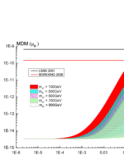
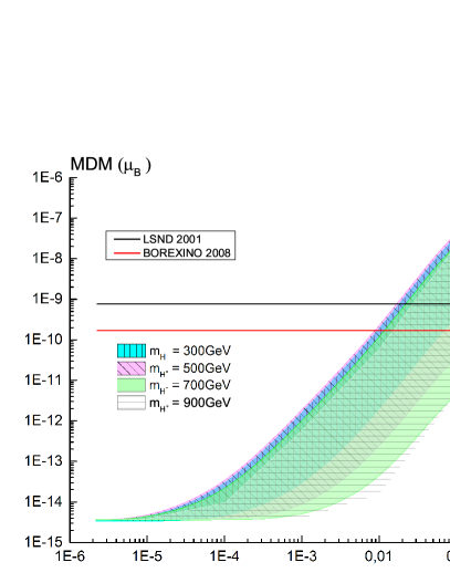
Figure 7: Values of the magnetic dipole moment (MDM) as a function of the muon neutrino mass between $\left(1\times 10^{-5}-4\times 10^{-1}\right)MeV$ and for values of the charged Higgs mass of $\left(100-300-500-700-900\right)GeV$ for the 2HDM type I and $\left(300-500-700-900\right)GeV$ for the 2HDM type II.

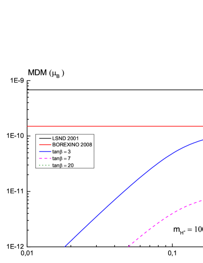
Figure 8: Values of the MDM as a function of the muon neutrino mass between $\left(1\times 10^{-2}-4\times 10^{-1}\right)MeV$ and for values of the charged Higgs mass of $100GeV$ for the 2HDM type I.

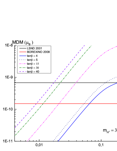
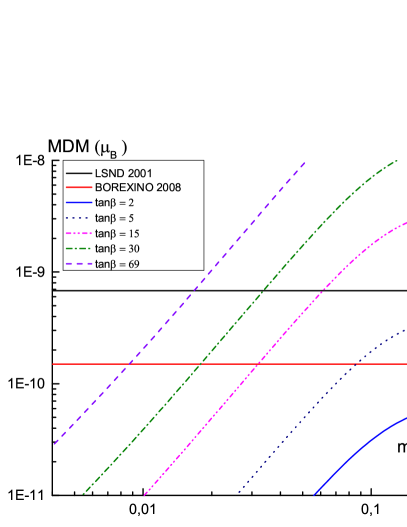
Figure 9: Values of the MDM as a function of the muon neutrino mass between $\left(1\times 10^{-3}-4\times 10^{-1}\right)MeV$ and for values of the charged Higgs mass of $\left(300-500-700-900\right)GeV$ to 2HDM type II

	$m_{H^{\pm}}\left(GeV\right)$
$\tan\beta$	$300$	$500$	$700$	$900$	Experiment
2	$-$	$-$	$-$	$-$	LSND 2001
	$-$	$3.31\times 10^{-1}$	$-$	$-$	BOREXINO 2008
4	$1.85\times 10^{-1}$	$-$	$-$	$-$	LSND 2001
	$6.47\times 10^{-2}$	$-$	$-$	$-$	BOREXINO 2008
5	$1.16\times 10^{-1}$	$2.82\times 10^{-1}$	$-$	$-$	LSND 2001
	$5.3\times 10^{-2}$	$8.71\times 10^{-2}$	$2.18\times 10^{-1}$	$2.25\times 10^{-1}$	BOREXINO 2008
15	$3.95\times 10^{-2}$	$6.16\times 10^{-2}$	$8.64\times 10^{-2}$	$1.16\times 10^{-1}$	LSND 2001
	$2.07\times 10^{-2}$	$3.18\times 10^{-2}$	$4.26\times 10^{-2}$	$5.27\times 10^{-2}$	BOREXINO 2008
30	$2.2\times 10^{-2}$	$3.36\times 10^{-2}$	$4.51\times 10^{-2}$	$5.57\times 10^{-2}$	LSND 2001
	$1.15\times 10^{-2}$	$1.78\times 10^{-2}$	$2.39\times 10^{-2}$	$2.89\times 10^{-2}$	BOREXINO 2008
40	$1.72\times 10^{-2}$	$-$	$-$	$-$	LSND 2001
	$8.95\times 10^{-3}$	$-$	$-$	$-$	BOREXINO 2008
69	$-$	$1.67\times 10^{-2}$	$-$	$-$	LSND 2001
	$-$	$8.7\times 10^{-3}$	$-$	$-$	BOREXINO 2008
70	$-$	$-$	$2.19\times 10^{-2}$	$2.69\times 10^{-2}$	LSND 2001
	$-$	$-$	$1.15\times 10^{-2}$	$1.43\times 10^{-2}$	BOREXINO 2008

Table 3: This table shows upper bounds for the muon neutrino mass $\left(MeV\right)$ as a function the free parameters $\tan\beta$ and $m_{H^{\pm}}$ in the 2HDM type II, taken from figure 9. The empty cases correspond to excluded regions of the model.

In Fig. 7, we plot the muon neutrino mass versus MDM for the same charged Higgs masses as before for the 2HDM type I (left-hand side) and type II (right-hand side). The horizontal lines correspond to the experimental limits for MDM coming from LSND 2001(Liquid Scintillating Neutrino Detector)[20] which is $\mu_{\nu_{\mu}}<6.8\times 10^{-10}\mu_{B}$ at $90\%~{}C.L.$, and BOREXino 2008 (Boron solar neutrino experiment)[21] which is $\mu_{\nu_{\mu}}<1.9\times 10^{-10}\mu_{B}$ at $90\%~{}C.L.$.

From Fig. 7, we can see that it is necessary to make a more detailed analysis for certain values of the Higgs mass and the respective values of $\tan\beta$ for each model, in order to find upper limits for the neutrino mass as a function of charged Higgs masses, $\tan\beta$ and the current experimental limits. This more detailed analysis is shown in Fig. 8 for the 2HDM type I and in Fig. 9 for the 2HDM type II. We observe that in the 2HDM type I the strongest bound for the muon neutrino mass that we obtain is given by$~{}2.583\times 10^{-1}MeV\$for $M_{H^{+}}=100GeV\$and $\tan\beta=3$ obtained from the bound of MDM from BOREXino. Nevertheless, for the interval of neutrino mass plotted we do not obtain bounds on the neutrino mass from the bound of MDM coming from LSND, neither for other masses of the charged Higgs.

As for the 2HDM type II, we observe significant differences in the patterns of the bounds. For instance, in the 2HDM type II the hierarchy of the bounds are in opposite order as a function of $\tan\beta$ with respect to the 2HDM type I. This happens because in the 2HDM type I the couplings are proportional only to $\tan\beta$, while for the 2HDM type II the couplings are proportional to either $\tan\beta$ or $\cot\beta$. Of course, when the charged Higgs mass increases, the bounds on the muon neutrino mass become less restrictive since the contribution of the new physics tends to decouple as the Higgs mass increases.

Considering the current experimental limits, the strongest upper limit that could take the muon neutrino mass in the 2HDM type II is $8.953\times 10^{-3}MeV,\$obtained from the set of parameters $m_{H^{\pm}}=300GeV$ and $\tan\beta=40$. The numerical values of the upper bounds for the muon neutrino mass within the 2HDM type II, are shown in table 3 for different allowed values of $m_{H^{\pm}}$ and $\tan\beta$ parameters.

Figure 10: Values of the MDM as a function of the tau neutrino mass between $\left(1\times 10^{-6}-3\times 10^{1}\right)MeV$ and for values of the charged Higgs mass of $\left(100-300-500-700-900\right)GeV$ for the 2HDM type I and $\left(300-500-700-900\right)GeV$ for the 2HDM type II.

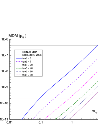
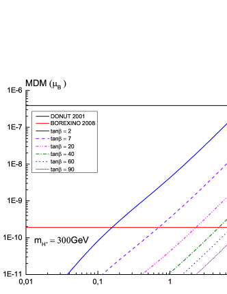
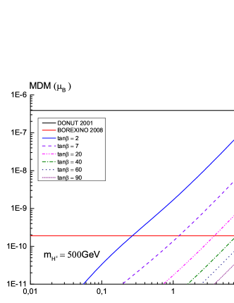
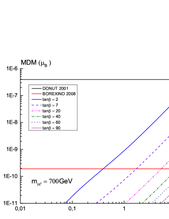
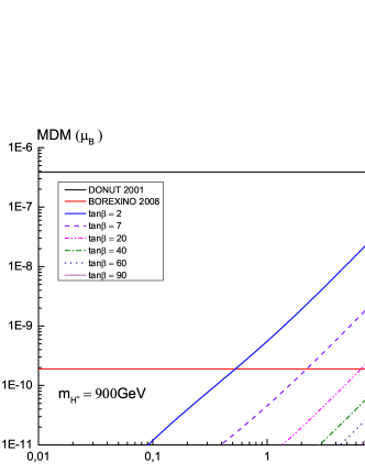
Figure 11: Values of the MDM as a function of the tau neutrino mass between $\left(1\times 10^{-2}-3\times 10^{1}\right)MeV$ and for values of the charged Higgs mass of $\left(100-300-500-700-900\right)GeV$ for the 2HDM type I.

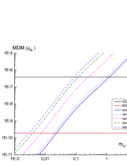
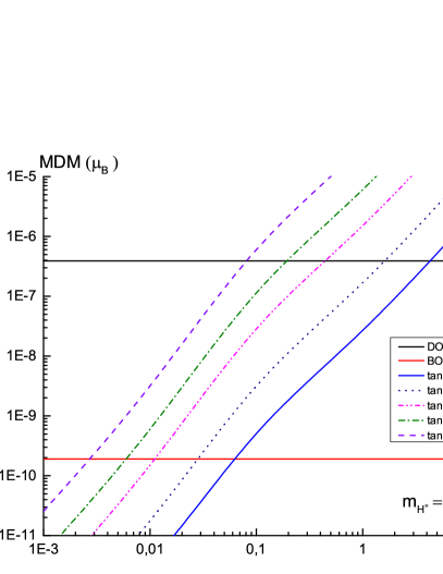
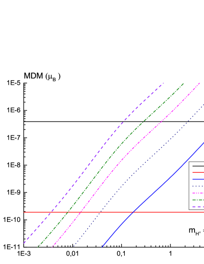
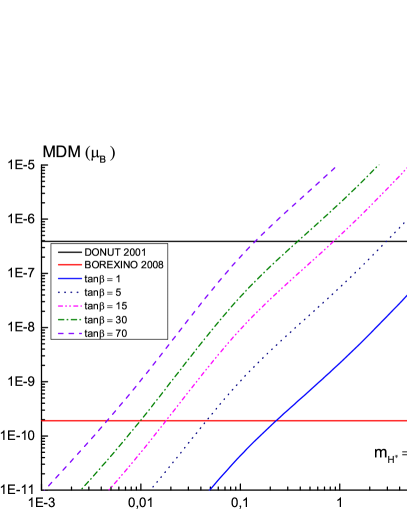
Figure 12: Values of the MDM as a function of the tau neutrino mass between $\left(1\times 10^{-3}-3\times 10^{1}\right)MeV$ and for values of the charged Higgs mass of $\left(300-500-700-900\right)GeV$ for the 2HDM type II

	$m_{H^{\pm}}\left(GeV\right)$
$\tan\beta$	$100$	$300$	$500$	$700$	$900$	Experiment
2	$-$	$10.95$	$17.42$	$23.95$	$29.78$	DONUT 2001
	$-$	$1.55$	$2.71\times 10^{-1}$	$3.95\times 10^{-1}$	$5.3\times 10^{-1}$	BOREXINO 2008
3	$6.28$	$-$	$-$	$-$	$-$	DONUT 2001
	$8.86\times 10^{-2}$	$-$	$-$	$-$	$-$	BOREXINO 2008
7	$16.67$	$-$	$-$	$-$	$-$	DONUT 2001
	$2.6\times 10^{-1}$	$7.08\times 10^{-1}$	$1.19$	$1.74$	$2.19$	BOREXINO 2008
20	$-$	$-$	$-$	$-$	$-$	DONUT 2001
	$7.74\times 10^{-1}$	$2.31$	$3.75$	$5.29$	$6.59$	BOREXINO 2008
40	$-$	$-$	$-$	$-$	$-$	DONUT 2001
	$1.72$	$4.84$	$7.69$	$10.4$	$13.07$	BOREXINO 2008
60	$-$	$-$	$-$	$-$	$-$	DONUT 2001
	$2.67$	$7.19$	$11.81$	$15.68$	$19.35$	BOREXINO 2008
90	$-$	$-$	$-$	$-$	$-$	DONUT 2001
	$4.05$	$10.95$	$17.42$	$23.64$	$29.4$	BOREXINO 2008

Table 4: This table shows the upper bounds for the tau neutrino mass $\left(MeV\right)$ for several allowed values of the free parameters $\tan\beta$ and $m_{H^{\pm}}$ in the 2HDM type I, taken from figure 11. The empty cases correspond to excluded regions of the model.

	$m_{H^{\pm}}\left(GeV\right)$
$\tan\beta$	$300$	$500$	$700$	$900$	Experiment
1	$-$	$-$	$11.87$	$15.65$	DONUT 2001
	$-$	$-$	$1.73\times 10^{-1}$	$2.27\times 10^{-1}$	BOREXINO 2008
2	$-$	$4.44$	$-$	$-$	DONUT 2001
	$-$	$6.24\times 10^{-2}$	$-$	$-$	BOREXINO 2008
4	$1.24$	$-$	$-$	$-$	DONUT 2001
	$2.27\times 10^{-2}$	$-$	$-$	$-$	BOREXINO 2008
5	$9.52\times 10^{-1}$	$1.58$	$2.27$	$2.97$	DONUT 2001
	$1.82\times 10^{-2}$	$2.77\times 10^{-2}$	$3.66\times 10^{-2}$	$4.52\times 10^{-2}$	BOREXINO 2008
15	$2.48\times 10^{-1}$	$4.58\times 10^{-1}$	$6.49\times 10^{-1}$	$8.63\times 10^{-1}$	DONUT 2001
	$7.13\times 10^{-3}$	$1.13\times 10^{-2}$	$1.43\times 10^{-2}$	$1.73\times 10^{-2}$	BOREXINO 2008
30	$1.14\times 10^{-1}$	$1.93\times 10^{-1}$	$2.89\times 10^{-1}$	$3.82\times 10^{-1}$	DONUT 2001
	$3.7\times 10^{-3}$	$5.82\times 10^{-3}$	$8.04\times 10^{-3}$	$9.62\times 10^{-3}$	BOREXINO 2008
40	$8.58\times 10^{-2}$	$-$	$-$	$-$	DONUT 2001
	$2.87\times 10^{-3}$	$-$	$-$	$-$	BOREXINO 2008
69	$-$	$8.14\times 10^{-2}$	$-$	$-$	DONUT 2001
	$-$	$2.71\times 10^{-3}$	$-$	$-$	BOREXINO 2008
70	$-$	$-$	$1.12\times 10^{-1}$	$1.39\times 10^{-1}$	DONUT 2001
	$-$	$-$	$3.57\times 10^{-3}$	$4.48\times 10^{-3}$	BOREXINO 2008

Table 5: Upper bounds for the tau neutrino mass $\left(MeV\right)$ for several allowed values of the free parameters $\tan\beta$ and $m_{H^{\pm}}$ in the 2HDM type II, taken from figure 12. The empty cases correspond to excluded regions of the model.

• Tau neutrino case

We shall plot within the interval $2\times 10^{-6}\leq m_{\nu_{\tau}}\leq 20MeV$, and obtain our bounds from the experimental limits on the MDM. In Fig. 10, we plot the tau neutrino mass versus MDM for the same charged Higgs masses as before for the 2HDM type I (left-hand side) and type II (right-hand side). The horizontal lines correspond to the experimental limits for MDM coming from DONUT 2001(Direct Observation of the NU Tau)[22] which is $\mu_{\nu_{\tau}}<3.9\times 10^{-7}\mu_{B}$ at $90\%~{}C.L.$, and BOREXino 2008[21] which is $\mu_{\nu_{\mu}}<1.5\times 10^{-10}\mu_{B}$ at $90\%~{}C.L$.

Figure 10 shows that we require a more detailed analysis of the upper bounds of the tau neutrino masses in terms of the free parameters. Such an analysis is carried out in Fig. 11 for the 2HDM type I and in Fig. 12 for the 2HDM type II. Once again we have significant differences in the patterns of the bounds for the models of type I and of type II because of the different behavior of the couplings with respect to the $\tan\beta$ parameter. Further, the upper limits of the tau neutrino mass is weakened as the charged Higgs mass increases owing to the decoupling behavior of the diagrams with respect to the Higgs mass.

Considering the current experimental limits, the strongest limit obtained for the tau neutrino mass in the 2HDM type I is$\ 9.098\times 10^{-2}MeV$, and occurs for the values $m_{H^{\pm}}=100GeV$ and $\tan\beta=3$. As for the 2HDM type II the strongest upper limit on the tau neutrino mass is $2.926\times 10^{-3}MeV$ obtained with the set of parameters $m_{H^{\pm}}=300GeV$ and $\tan\beta=40$. Finally, the numerical values of the upper bounds for the muon neutrino mass within the 2HDM type I and II, are shown in tables 4 and 5 respectively, for different allowed values of $m_{H^{\pm}}$ and $\tan\beta$ parameters.

7 Conclusions

The neutrino magnetic moment provides a tool for exploration of physics beyond the Standard Model. The magnitude of the magnetic moment is highly sensitive to the neutrino mass, but also depends on the mass of the associated charged lepton inserted into the loops.

Further, the value of the magnetic moments of the neutrinos could be modified with physics beyond the Standard Model. In particular for the Two Higgs Doublet Model (2HDM) we evaluated the contributions coming from the insertion of the charged Higgs boson into the loops. Our results show that for the 2HDM of type I and of type II, the total contribution is far from the threshold of experimental detection in the case of electron neutrinos (owing to the supression coming from the electron mass into the loops), obtaining a maximum contribution about six orders of magnitude below the present experimental limits. In the case of muon neutrinos the total contribution produces weak bounds for the mass of the neutrinos for model type I, and stronger bounds for the case of model type II. Finally, such bounds are much stronger for tau neutrinos (because of the enhancement of the tau mass into the loops) for either type of 2HDM, but restrictions are much stronger for the model type II.

In general since the bounds are highly sensitive to the value of the $\tan\beta$ parameter, the limits obtained are significantly different for the model type I with respect to the model type II because of the different dependence on the Yukawa couplings of each model with $\tan\beta$. Of course, the limits are weakened as the mass of the charged Higgs increases since the contribution of new physics tends to decouple as the Higss mass grows. Further, since the contribution of diagrams involving the associated charged lepton increases with the mass of the charged lepton, the strongest bounds are obtained for the neutrino associated with the heaviest charged lepton (tau neutrino) while basically no bounds near the experimental threshold are obtained for the electron neutrino.

8 Acknowledgments

We acknowledge to Division de Investigacion de Bogotá (DIB) for its financial support and the Universidad Manuela Beltran.

Appendix A Explicit expressions for the EFF

In this Appendix we present some details of the process of calculating the EFF’s. For the case of two higgs bosons and one lepton $\left(2H^{\pm}1L\right)$, the general form of the contribution can be written as

$$\Lambda_{2H^{\pm}1L}^{\alpha}\left(q,l\right)=-e\int\frac{d^{4}k}{\left(2\pi\right)^{4}}\left\{\frac{\left(2k^{\alpha}+p_{2}^{\alpha}+p_{1}^{\alpha}\right)\left(aP_{L}+bP_{R}\right)\left(\not{k}+m_{l}\right)\left(cP_{L}+dP_{R}\right)}{\left[\left(k+p_{1}\right)^{2}-m_{H^{\pm}}^{2}\right]\left[\left(k+p_{2}\right)^{2}-m_{H^{\pm}}^{2}\right]\left(k^{2}-m_{l}^{2}\right)}\right\}$$

expanding the numerator, denoting $A=\left(aP_{L}+bP_{R}\right)$ and $B=\left(cP_{L}+dP_{R}\right)$ we find

$$\left(2k^{\alpha}+p_{2}^{\alpha}+p_{1}^{\alpha}\right)A\left(\not{k}+m_{l}\right)B=\left(2k^{\alpha}k_{\beta}+p_{2}^{\alpha}k_{\beta}+p_{1}^{\alpha}k_{\beta}\right)A\gamma^{\beta}B+m_{l}\left(2k^{\alpha}+p_{2}^{\alpha}+p_{1}^{\alpha}\right)AB$$

and for the denominator we use the dimensional regularization method

$$\frac{1}{\underset{a_{1}}{\underbrace{\left[\left(k+p_{2}\right)^{2}-m_{H^{\pm}}^{2}\right]}}\underset{a_{2}}{\underbrace{\left(k^{2}-m_{l}^{2}\right)}}\underset{a_{3}}{\underbrace{\left[\left(k+p_{1}\right)^{2}-m_{H^{\pm}}^{2}\right]}}}$$

then

$$\frac{1}{a_{1}^{1}a_{2}^{1}a_{3}^{1}} = \frac{\Gamma\left(1+1+1\right)}{\Gamma\left(1\right)\Gamma\left(1\right)\Gamma\left(1\right)}\int\limits_{0}^{1}dx\int\limits_{0}^{x}dy\frac{\left(x_{0}-x\right)^{\left(1-1\right)}\left(x-y\right)^{\left(1-1\right)}\left(y-x_{3}\right)^{\left(1-1\right)}}{\left[a_{3}\left(x_{0}-x\right)+a_{2}\left(x-y\right)+a_{1}\left(y-x_{3}\right)\right]^{3}}$$

$$= \Gamma\left(3\right)\int\limits_{0}^{1}dx\int\limits_{0}^{x}dy\frac{1}{\left[\left(\left(k+p_{1}\right)^{2}-m_{H^{\pm}}^{2}\right)\left(1-x\right)+\left(k^{2}-m_{l}^{2}\right)\left(x-y\right)+\left[\left(k+p_{2}\right)^{2}-m_{H^{\pm}}^{2}\right]y\right]^{3}}$$

where $x_{0}=1$ and $x_{3}=0$. Thus, the denominator can be written as

$$\left[\left(k+p_{1}\right)^{2}-m_{H^{\pm}}^{2}\right]\left(1-x\right)+\left(k^{2}-m_{l}^{2}\right)\left(x-y\right)+\left[\left(k+p_{2}\right)^{2}-m_{H^{\pm}}^{2}\right]y$$

$$= k^{2}+2k\cdot\underset{b}{\underbrace{\left(p_{1}\left(1-x\right)+p_{2}y\right)}}+\underset{a^{2}}{\underbrace{\left(m_{H^{\pm}}^{2}-m_{\nu}^{2}-m_{l}^{2}\right)x+\left(m_{l}^{2}+m_{\nu}^{2}-m_{H^{\pm}}^{2}\right)y+m_{\nu}^{2}-m_{H^{\pm}}^{2}}}$$

$$= k^{2}+2k\cdot b+a^{2}$$

$$= k^{2}+P^{2}$$

where we use the transformation $k\rightarrow k-b$ in the last equation and

$$P^{2}=a^{2}-b^{2}=y^{2}m_{\nu}^{2}-2xym_{\nu}^{2}+\left(m_{\nu}^{2}-m_{l}^{2}+m_{H^{\pm}}^{2}\right)y+x^{2}m_{\nu}^{2}+\left(m_{l}^{2}-m_{\nu}^{2}-m_{H^{\pm}}^{2}\right)x+m_{H^{\pm}}^{2}$$

in consequence, adding the corresponding terms to the integral with terms in the numerator $1,k^{\mu}$ and $k^{\mu}k_{\nu}$ we obtain

$$\Lambda_{2H^{\pm}1L}^{\alpha}\left(q,l\right) = -e\int\frac{d^{4}k}{\left(2\pi\right)^{4}}\left\{\frac{\left(2k^{\alpha}k_{\beta}+p_{2}^{\alpha}k_{\beta}+p_{1}^{\alpha}k_{\beta}\right)A\gamma^{\beta}B+m_{l}\left(2k^{\alpha}+p_{2}^{\alpha}+p_{1}^{\alpha}\right)AB}{\left[\left(k+p_{1}\right)^{2}-m_{H^{\pm}}^{2}\right]\left[\left(k+p_{2}\right)^{2}-m_{H^{\pm}}^{2}\right]\left(k^{2}-m_{l}^{2}\right)}\right\}$$

$$= -e\frac{i}{16\pi^{2}}\int\limits_{0}^{1}dx\int\limits_{0}^{x}dy\left[\left(-\frac{2b^{\alpha}b^{\beta}}{P^{2}}+g^{\alpha\beta}\ln\frac{\Lambda^{2}}{P^{2}}+\frac{p_{2\alpha}b^{\beta}}{P^{2}}+\frac{p_{1_{\alpha}}b^{\beta}}{P^{2}}\right)A\gamma^{\beta}B+\left(\frac{2b^{\alpha}}{P^{2}}-\frac{p_{2\alpha}}{P^{2}}-\frac{p_{1\alpha}}{P^{2}}\right)m_{l}AB\right]$$

expanding the terms $b^{\mu}$ and employing the Dirac equation

$$\left(\gamma\cdot p_{1}-m\right)u\left(p_{1}\right) = 0\Rightarrow\not{p}u\left(p_{1}\right)=mu\left(p_{1}\right)$$

$$\bar{u}\left(p_{2}\right)\left(\gamma\cdot p_{2}-m\right) = 0\Rightarrow\bar{u}\left(p_{2}\right)\not{p}_{2}=m\bar{u}\left(p_{2}\right)$$

then

$$\Lambda_{2H^{\pm}1L}^{\alpha}\left(q,l\right)$$

$$= -e\frac{i}{16\pi^{2}}\int\limits_{0}^{1}dx\int\limits_{0}^{x}dy\left[\left(-\frac{2b^{\alpha}b^{\beta}}{P^{2}}+g^{\alpha\beta}\ln\frac{\Lambda^{2}}{P^{2}}+\frac{p_{2\alpha}b^{\beta}}{P^{2}}+\frac{p_{1_{\alpha}}b^{\beta}}{P^{2}}\right)A\gamma^{\beta}B+\left(\frac{2b^{\alpha}}{P^{2}}-\frac{p_{2\alpha}}{P^{2}}-\frac{p_{1\alpha}}{P^{2}}\right)m_{l}AB\right]$$

$$= -e\frac{i}{16\pi^{2}}\int\limits_{0}^{1}dx\int\limits_{0}^{x}dy\left[\frac{1}{P^{2}}\left(\left[\begin{array}[]{c}-p_{1\alpha}\left(1-x\right)^{2}-p_{2\alpha}y\left(1-x\right)-p_{1\alpha}\left(1-x\right)y-p_{2\alpha}y^{2}\\ +\left(p_{2\alpha}\left(1-x\right)+p_{2\alpha}y\right)\frac{1}{2}+\left(p_{1\alpha}\left(1-x\right)+p_{1\alpha}y\right)\frac{1}{2}\end{array}\right]m_{\nu}\left(\left(ac+bd\right)+\left(bd-ac\right)\gamma_{5}\right)\right.\right.$$

$$\left.\left.+m_{l}\left[p_{1\alpha}\left(1-x\right)+p_{2\alpha}y-p_{2\alpha}\frac{1}{2}-p_{1\alpha}\frac{1}{2}\right]\left[\left(ac+bd\right)+\left(bd-ac\right)\gamma_{5}\right]\right)+\frac{1}{2}\gamma^{\alpha}\left[\left(bc+ad\right)-\left(bc-ad\right)\gamma_{5}\right]\ln\left(\frac{\Lambda^{2}}{P^{2}}\right)\right]$$

and using the Gordon relation

$$\overline{u}\left(p_{2\alpha}\right)\gamma_{\alpha}u\left(p_{1\alpha}\right) = \frac{1}{2m_{\nu}}\overline{u}\left(p_{2\alpha}\right)\left[\left(p_{2}+p_{1}\right)_{\alpha}+i\sigma^{\alpha\mu}q_{\mu}\right]u\left(p_{1\alpha}\right)$$

$$\Rightarrow \overline{u}\left(p_{2\alpha}\right)\left(p_{2}+p_{1}\right)_{\alpha}u\left(p_{1\alpha}\right)=\overline{u}\left(p_{2\alpha}\right)2m_{\nu}\gamma_{\alpha}u\left(p_{1\alpha}\right)-\overline{u}\left(p_{2\alpha}\right)i\sigma^{\alpha\mu}q_{\mu}u\left(p_{1\alpha}\right)$$

finally the contribution for the EFF’s with two charged Higgses and one lepton can be represented by

$$\Lambda_{2H^{\pm}1L}^{\alpha}\left(q,l\right)=$$

$$\frac{-ie}{16\pi^{2}}\int\limits_{0}^{1}dx\int\limits_{0}^{x}dy\left[\frac{1}{P^{2}}\left(\left(\left(m_{l}m_{\nu}-2m_{\nu}^{2}\right)\gamma_{\alpha}+x\left(6m_{\nu}^{2}-2m_{\nu}m_{l}\right)\gamma_{\alpha}-4x^{2}m_{\nu}^{2}\gamma_{\alpha}+\left(m_{\nu}-\frac{1}{2}m_{l}\right)i\sigma^{\alpha\mu}q_{\mu}\right.\right.\right.$$

$$\left.\left.+\left(m_{l}-3m_{\nu}\right)ix\sigma^{\alpha\mu}q_{\mu}+2x^{2}im_{\nu}\sigma^{\alpha\mu}q_{\mu}\right)\left[\left(ac+bd\right)+\left(bd-ac\right)\gamma_{5}\right]+\frac{1}{2}\gamma^{\alpha}\left[\left(bc+ad\right)-\left(bc-ad\right)\gamma_{5}\right]\ln\left(\frac{\Lambda^{2}}{P^{2}}\right)\right]$$

And for the case of two lepton and a charged Higgs $\left(2L1H^{\pm}\right)$ the general form of the contribution can be written as

$$\Lambda_{2L1H^{\pm}}^{\alpha}\left(q,l\right)=-e\int\frac{d^{4}k}{\left(2\pi\right)^{4}}\left\{\frac{\left(aP_{L}+bP_{R}\right)\left(\not{k}+\not{p}_{1}+m_{l}\right)\gamma^{\alpha}\left(\not{k}+\not{p}_{2}+m_{l}\right)\left(cP_{L}+dP_{R}\right)}{\left[\left(k+p_{1}\right)^{2}-m_{l}^{2}\right]\left[\left(k+p_{2}\right)^{2}-m_{l}^{2}\right]\left(k^{2}-m_{H^{+}}^{2}\right)}\right\}$$

expanding the numerator and using the same change as for the vertex $2H^{\pm}1L$ we have

$$\left.A\left(\not{k}+\not{p}_{1}+m_{l}\right)\gamma^{\alpha}\left(\not{k}+\not{p}_{2}+m_{l}\right)B=\right.$$

$$\left(k_{\mu}k_{\beta}+p_{1\mu}k_{\beta}+k_{\mu}p_{2\beta}+p_{1\mu}p_{2\beta}\right)A\gamma^{\mu}\gamma^{\alpha}\gamma^{\beta}B+m_{l}\left(k+p_{1}\right)_{\mu}A\gamma^{\mu}\gamma^{\alpha}B+m_{l}\left(k+p_{2}\right)_{\beta}A\gamma^{\alpha}\gamma^{\beta}B+m_{l}^{2}A\gamma^{\alpha}B$$

and for the denominator we use the dimensional regularization method

$$\frac{1}{\underset{a_{1}}{\underbrace{\left[\left(k+p_{2}\right)^{2}-m_{l}^{2}\right]}}\underset{a_{2}}{\underbrace{\left(k^{2}-m_{H^{\pm}}^{2}\right)}}\underset{a_{3}}{\underbrace{\left[\left(k+p_{1}\right)^{2}-m_{l}^{2}\right]}}}$$

then

$$\frac{1}{a_{1}^{1}a_{2}^{1}a_{3}^{1}}=\Gamma\left(3\right)\int\limits_{0}^{1}dx\int\limits_{0}^{x}dy\frac{1}{\left[\left(\left(k+p_{1}\right)^{2}-m_{l}^{2}\right)\left(1-x\right)+\left(k^{2}-m_{H^{\pm}}^{2}\right)\left(x-y\right)+\left(\left(k+p_{2}\right)^{2}-m_{l}^{2}\right)y\right]^{3}}$$

where $x_{0}=1$ and $x_{3}=0$. Hence, the denominator can be written as

$$\left[\left(k+p_{1}\right)^{2}-m_{l}^{2}\right]\left(1-x\right)+\left(k^{2}-m_{H^{\pm}}^{2}\right)\left(x-y\right)+\left[\left(k+p_{2}\right)^{2}-m_{l}^{2}\right]y$$

$$= k^{2}+2k\cdot\underset{b}{\underbrace{\left(p_{1}\left(1-x\right)+p_{2}y\right)}}+\underset{a^{2}}{\underbrace{\left(m_{l}^{2}-m_{\nu}^{2}-m_{H^{\pm}}^{2}\right)x+\left(m_{H^{\pm}}^{2}+m_{\nu}^{2}-m_{l}^{2}\right)y+m_{\nu}^{2}-m_{l}^{2}}}$$

$$= k^{2}+2k\cdot b+a^{2}$$

$$= k^{2}+P^{2}$$

where we use the transformation $k\rightarrow k-b$ in the last equation and

$$P^{2}=a^{2}-b^{2}=y^{2}m_{\nu}^{2}-\left(m_{H^{\pm}}^{2}-m_{\nu}^{2}-m_{l}^{2}\right)y-2xym_{\nu}^{2}+x^{2}m_{\nu}^{2}-\left(m_{l}^{2}+m_{\nu}^{2}-m_{H^{\pm}}^{2}\right)x+m_{l}^{2}$$

therefore, adding the corresponding terms to the integral with terms $1,k^{\mu}$ and $k^{\mu}k_{\nu}$ in the numerator, we obtain

$$\Lambda_{2L1H^{\pm}}^{\alpha}\left(q,l\right)$$

$$= -e\int\frac{d^{4}k}{\left(2\pi\right)^{4}}\left\{\frac{\left(\left(k_{\mu}k_{\beta}+p_{1\mu}k_{\beta}+k_{\mu}p_{2\beta}+p_{1\mu}p_{2\beta}\right)A\gamma^{\mu}\gamma^{\alpha}\gamma^{\beta}B+m_{l}\left(k+p_{1}\right)_{\mu}A\gamma^{\mu}\gamma^{\alpha}B+m_{l}\left(k+p_{2}\right)_{\beta}A\gamma^{\alpha}\gamma^{\beta}B+m_{l}^{2}A\gamma^{\alpha}B\right)}{\left[\left(k+p_{1}\right)^{2}-m_{l}^{2}\right]\left[\left(k+p_{2}\right)^{2}-m_{l}^{2}\right]\left(k^{2}-m_{H^{\pm}}^{2}\right)}\right\}$$

$$= -e\frac{i}{16\pi^{2}}\int\limits_{0}^{1}dx\int\limits_{0}^{x}dy\left[\left(-\frac{b^{\mu}b^{\beta}}{P^{2}}+\frac{g^{\mu\beta}}{2}\ln\frac{\Lambda^{2}}{P^{2}}+\frac{p_{1\mu}b^{\beta}}{P^{2}}+\frac{p_{2_{\beta}}b^{\mu}}{P^{2}}-\frac{p_{1\mu}p_{2_{\beta}}}{P^{2}}\right)A\gamma^{\mu}\gamma^{\alpha}\gamma^{\beta}B\right.$$

$$\left.+\left(\frac{b^{\mu}}{P^{2}}-\frac{p_{1\mu}}{P^{2}}\right)m_{l}A\gamma^{\mu}\gamma^{\alpha}B+\left(\frac{b^{\beta}}{P^{2}}-\frac{p_{2\beta}}{P^{2}}\right)m_{l}A\gamma^{\alpha}\gamma^{\beta}B-\frac{1}{P^{2}}m_{l}^{2}A\gamma^{\alpha}B\right]$$

expanding the terms $b^{\mu}$ and employing the Dirac equation we obtain

$$\Lambda_{2L1H^{\pm}}^{\alpha}\left(q,l\right)$$

$$= -e\frac{i}{16\pi^{2}}\int\limits_{0}^{1}dx\int\limits_{0}^{x}dy\left[\left(-\frac{b^{\mu}b^{\beta}}{P^{2}}+\frac{g^{\mu\beta}}{2}\ln\frac{\Lambda^{2}}{P^{2}}+\frac{p_{1\mu}b^{\beta}}{P^{2}}+\frac{p_{2_{\beta}}b^{\mu}}{P^{2}}-\frac{p_{1\mu}p_{2_{\beta}}}{P^{2}}\right)A\gamma^{\mu}\gamma^{\alpha}\gamma^{\beta}B+\left(\frac{b^{\mu}}{P^{2}}-\frac{p_{1\mu}}{P^{2}}\right)m_{l}A\gamma^{\mu}\gamma^{\alpha}B\right.$$

$$\left.+\left(\frac{b^{\beta}}{P^{2}}-\frac{p_{2\beta}}{P^{2}}\right)m_{l}A\gamma^{\alpha}\gamma^{\beta}B-\frac{1}{P^{2}}m_{l}^{2}A\gamma^{\alpha}B\right]$$

$$= -e\frac{i}{16\pi^{2}}\int\limits_{0}^{1}dx\int\limits_{0}^{x}dy\left[\frac{1}{P^{2}}\left(\frac{1}{2}\left(x^{2}-2xy+2x+y^{2}-y\right)m_{\nu}^{2}\gamma^{\alpha}\left(\left(bc+ad\right)-\left(bc-ad\right)\gamma_{5}\right)\right.\right.$$

$$+\left(\left(y-x+xy\right)\left(p_{2\alpha}+p_{1\alpha}\right)-p_{2\alpha}y^{2}+p_{1\alpha}\left(x-y-x^{2}\right)\right)m_{\nu}\left(\left(ac+bd\right)+\left(bd-ac\right)\gamma_{5}\right)$$

$$m_{l}m_{\nu}\gamma^{\alpha}\left(\left(bc+ad\right)-\left(bc-ad\right)\gamma_{5}\right)+m_{l}\left(p_{2\alpha}\left(y-1\right)-xp_{1\alpha}\right)\left(\left(ac+bd\right)+\left(bd-ac\right)\gamma_{5}\right)$$

$$\left.\left.-m_{l}^{2}\frac{1}{2}\gamma^{\alpha}\left(\left(bc+ad\right)-\left(bc-ad\right)\gamma_{5}\right)\right)-\frac{1}{2}\gamma^{\alpha}\left(\left(bc+ad\right)-\left(bc-ad\right)\gamma_{5}\right)\ln\frac{\Lambda^{2}}{P^{2}}\right)$$

and using the Gordon relation like in the previous case, the contribution to the EFF’s with two leptons and one charged Higgs can be represented as

$$\Lambda_{2L1H^{\pm}}^{\alpha}\left(q,l\right)=$$

$$\frac{-ie}{16\pi^{2}}\int\limits_{0}^{1}dx\int\limits_{0}^{x}dy\left(\frac{1}{P^{2}}\left(\begin{array}[]{c}\left(2x^{2}m_{\nu}^{2}-\frac{1}{2}xm_{\nu}^{2}+m_{l}m_{\nu}-\frac{1}{2}m_{l}^{2}\right)\gamma^{\alpha}\left(\left(bc+ad\right)-\left(bc-ad\right)\gamma_{5}\right)\\ +\left(2x\left(m_{\nu}^{2}-m_{l}m_{\nu}\right)-4m_{\nu}^{2}x^{2}\right)\gamma_{\alpha}\left(\left(ac+bd\right)+\left(bd-ac\right)\gamma_{5}\right)\end{array}\right.\right.$$

$$\left.\left.+\left(2x^{2}m_{\nu}i\sigma^{\alpha\mu}q_{\mu}+m_{l}xi\sigma^{\alpha\mu}q_{\mu}-xm_{\nu}i\sigma^{\alpha\mu}q_{\mu}\right)\left[\left(ac+bd\right)+\left(bd-ac\right)\gamma_{5}\right]\right)-\frac{1}{2}\gamma^{\alpha}\left[\left(bc+ad\right)-\left(bc-ad\right)\gamma_{5}\right]\ln\frac{\Lambda^{2}}{P^{2}}\right)$$

References

[1] Y. Fukuda et al. (Super-Kamiokande Collaboration) Phys.
Rev. Lett. 81, 1562 (1998).
[2] K. Abe et al. (T2K Collaboration), PRL 112, 061802 (2014)
[3] J. Beringer et al. (Particle Data Group), Phys. Rev. D86,
010001 (2013)
[4] S. Mereghetti, Astron. Astrophys. Rev. 15, 225 (2008);
[5] G.C. Branco, P.M. Ferreira, L. Lavoura, M.N. Rebelo, Marc
Sher, Joao P. Silva, Theory and phenomenology of two-Higgs-doublet models,
Physics reports 516 (2012).
[6] B. Pontecorvo, Journal of Experimental and Theoretical
Physics 26, 984 (1983);
[7] Z. Maki, M. Nakagawa, S. Sakata, Progress of Theoretical
Physics 28, 870, (1962);
[8] M. Nowakowski, E. A. Paschos, J. M. Rodriguez, Eur. J. Phys.
26 (2005) 545
[9] Broggini, C., C. Giunti, and A. Studenikin,
Electromagnetic properties of neutrinos, Adv. High Energy Phys. 2012,
459526, arXiv:1207.3980 [hep-ph]
[10] Carlo Giunti, Alexander Studenikin. Neutrino
electromagnetic properties,[arXiv:1006.1502v1 [hep-ph]].
[11] Lepton dipole moments (ed B. Roberts, J. Marciano) world
Scientific, (2010);
[12] J. Gunion, H. Haber, G. Kane, S. Dawson. Higgs hunters guide,
Perseus publishing. (2000);
[13] R. A. Diaz, Ph.D. Thesis [arXiv: hep-ph/0212237].
[14] M. Carena, H. Haber. Higgs Boson Theory and Phenomenology,
Prog. Part. Nucl. Phys. 50, 63 (2003). [arXiv:hep/ph/0208209]
[15] K. Fujikawa, R. Shrock, The Magnetic Moment of a Massive
Neutrino and Neutrino Spin Rotation, Phys. Rev. Lett. 45 (1980) 963.
[16] A.G. Akeroyd and F. Mahmoudi, Constraints on charged
Higgs bosons from and , JHEP04(2009)121
[17] F. Mahmoudi and O. Stål, Flavor constraints on
two-Higgs-doublet models with general diagonal Yukawa couplings, Phys. Rev.
D 81, 035016, (2010)
[18] H. Wong, et al., A Search of Neutrino Magnetic Moments with a
High-Purity Germanium Detector at the Kuo-Sheng Nuclear Power Station,
Phys.Rev. D75 (2007) 012001.
[19] A. Beda, V. Brudanin, V. Egorov, D. Medvedev, V. Pogosov, et
al., Gemma experiment: The results of neutrino magnetic moment search,
Phys.Part.Nucl.Lett. 10 (2013) 139-143.
[20] L. B. Auerbach, R. L. Burman, D. O. Caldwell et al.,
Measurement of electron-neutrino electron elastic scattering, Physcial
Review D, vol. 63, no. 11, 11 pages, 2001.
[21] D. Montanino, M. Picariello, and J. Pulido, Probing
neutrino magnetic moment and unparticle interactions with Borexino, Physical
Review D, vol. 77, no. 9, Article ID 093011, 9 pages, 2008.
[22] R. Schwienhorst, D. Ciampa, C. Erickson et al., A new
upper limit for the tau-neutrino magnetic moment, Physics Letters B, vol.
513, no. 1-2, pp. 23–29, 2001.