Route to hyperchaos in Rayleigh-Bénard convection

Abstract

Transition to hyperchaotic regimes in Rayleigh-Bénard convection in a square periodicity cell is studied by three-dimensional numerical simulations. By fixing the Prandtl number at $P=0.3$ and varying the Rayleigh number as a control parameter, a bifurcation diagram is constructed where a route to hyperchaos involving quasiperiodic regimes with two and three incommensurate frequencies, multistability, chaotic intermittent attractors and a sequence of boundary and interior crises is shown. The three largest Lyapunov exponents exhibit a linear scaling with the Rayleigh number and are positive in the final hyperchaotic attractor. Thus, a route to weak turbulence is found.

1 Introduction

Thermal convection refers to the motion of a heat-conducting fluid due to the presence of temperature differences. Convective flows are of interest in many areas ranging from technological processes (cooling of electronic devices, drying, material processing) to natural phenomena (convection in the terrestrial atmosphere, oceans, mantle, outer core and stellar convection). Origin of magnetic fields of many astrophysical objects is explained in the framework of the dynamo theory [1], where magnetic fields are generated by convective motions of electrically conducting fluids in their interior; chaotic convective flows play an important role in the fast dynamo theory.

Thermal convection in the dimensionless form is characterised by the Rayleigh number (Ra), that measures the magnitude of thermal buoyancy force, and the Prandtl number ($P$), the ratio of kinematic viscosity to thermal diffusivity. In the context of Astrophysics, values of the Prandtl number vary from small (for the solar convective zone, $P\sim 10^{-7}$ [2]) to large (for mantle convection, $P\sim 10^{23}$ [3]) values. The Prandtl number for the terrestrial outer core has intermediate values estimated to be between $0.1$ and $0.5$ [4, 5], however, in many terrestrial convective dynamo simulations a larger value ($P\sim 1$) is employed (see, e.g., [6] and references therein) using the argument that it expresses the “effective” or ”turbulent” value of the diffusivity [7].

In the dynamo theory, interest in the use of realistic values for the Prandtl number was enhanced by the following findings. Varying the value of the Prandtl number from 0.1 to 10 was found to have a strong influence on the morphology and dynamics of convection in the Earth’s outer core [8]. Strong dependence of the magnetic fields generated by convective flows on the value of the Prandtl number was found for $0.2\leq P\leq 5$ [9]. In [10], moderately low Prandtl numbers were beneficial for magnetic field generation in rotating spherical shells and special attention was devoted to dynamos for $P=0.1$. Analysis of the kinematic dynamo problem in [11] showed that convective attractors for $P=0.3$ are beneficial for the magnetic field generation (in comparison to the attractors for $P=1$ and 6.8).

Most of the convective flows in nature are turbulent. Thermal convection in a plane horizontal layer, called Rayleigh-Bénard convection, has been used for decades as one of the simplest examples of realistic hydrodynamic systems driven out of equilibrium where the simple flow becomes complex (turbulent) in a variety of bifurcation sequences, revealing different mechanisms of instability and demonstrating many common nonlinear dynamics phenomena, e.g., spontaneous symmetry breaking, pattern formation, intermittency, synchronisation, etc. (for a review, see [12, 13]). A common approach to study transition to turbulence in the framework of the dynamical systems theory is to study the evolution from simple non-chaotic (steady, time-periodic and quasiperiodic) attractors of the convective system to the chaotic ones. In chaotic attractors, trajectories are sensitive to initial conditions, i.e., initially close trajectories diverge in time, which is quantitatively characterised by the Lyapunov spectrum. Turbulent systems usually display hyperchaos, i.e., more than one positive Lyapunov exponent.

There is a wide range of works on bifurcation analysis of Rayleigh-Bénard convection as a function of Ra and $P$, most of which are devoted to the formation and destabilisation of steady planar convective rolls [14, 15, 16, 17] and transition to chaos [18, 11]. In [19], a bifurcation diagram is presented where a series of steady states representing different patterns is numerically obtained as a function of Ra in a small cylindrical domain. Also in cylindrical domains, hyperchaotic states were found in studies of spiral defect chaos using simulations of three-dimensional Rayleigh-Bénard convection, where the spectrum of Lyapunov exponents was used to quantify extensivity in spatiotemporal chaos [20, 21].

Still regarding transition to hyperchaos in Rayleigh-Bénard convection, in [22], a square periodicity cell with aspect ratio $L=2\sqrt{2}$ and stress-free boundaries was studied for $P=6.8$ in two-dimensional convection for Ra up to 32875 using a low-dimensional model (16 Fourier modes); the sequence of regimes is as follows: time-periodic, quasiperiodic with two basic frequencies, phase-locked (periodic) and then chaotic state (some of the chaotic states are hyperchaotic with two positive Lyapunov exponents).

In this letter we study the transition to hyperchaotic regimes (also referred to as transition to weak turbulence [23]) in three-dimensional Rayleigh-Bénard convection for $P=0.3$ in a square convective cell for Ra increasing from 1720 (time-periodic state) to 2500 (hyperchaotic state). We show that a sequence of crises involving quasiperiodic and chaotic attractors, as well as chaotic saddles, is responsible for the evolution of the attractors of the system from periodic convective states to hyperchaos with at least three positive Lyapunov exponents.

2 Statement of the problem and solution

A Newtonian fluid flow in a horizontal plane layer is considered, where the fluid is uniformly heated from below and cooled from above. Fluid flow is buoyancy-driven and the Boussinesq approximation is assumed. We adopt the vertical size of the layer as a length scale, the vertical heat diffusion time as a time scale, and the vertical temperature gradient as a temperature scale. Then, in a Cartesian reference frame with the orthonormal basis $({\bf e}_{1},{\bf e}_{2},{\bf e}_{3})$, where ${\bf e}_{3}$ is opposite to the direction of gravity, the equations governing the convective system are (see, e.g., [15]):

$${\partial{\bf v}}/{\partial t}=P\nabla^{2}{\bf v}+{\bf v}\times(\nabla\times{\bf v})+P{\rm Ra}\theta{\bf e}_{3}-\nabla p,$$ (1)

$${\partial\theta}/{\partial t}=\nabla^{2}\theta-({\bf v}\cdot\nabla)\theta+v_{3},$$ (2)

$$\nabla\cdot{\bf v}=0,$$ (3)

where ${\bf v}({\bf x},t)=(v_{1},v_{2},v_{3})$ is the fluid velocity, $p({\bf x},t)$ the pressure, and $\theta({\bf x},t)=T({\bf x},t)-(T_{1}+(T_{2}-T_{1})x_{3})$ is the difference between the temperature $T$ and its linear profile. Temperatures of the horizontal boundaries at the bottom, $T_{1}$, and top, $T_{2}$, are maintained constant, with $T_{1}>T_{2}$. Here, the spatial coordinates are ${\bf x}=(x_{1},x_{2},x_{3})$ and $t$ stands for time. The non-dimensional parameters are the Prandtl number, $P$, and the Rayleigh number, Ra.

The horizontal boundaries of the layer are assumed to be stress-free, $\partial v_{1}/\partial x_{3}=\partial v_{2}/\partial x_{3}=v_{3}=0$, and maintained at constant temperatures, $\theta=0$. A square convective cell is considered, ${\bf x}\in[0,L]^{2}\times[0,1]$, and all the fields are periodic in the horizontal directions, $x_{1}$ and $x_{2}$, with period $L$. The linear theory [14] suggests that at the onset of convection in an infinite layer (Ra_c=657.5 for the boundary conditions under consideration) the critical horizontal wavenumber is $\pi/\sqrt{2}$, independently of the Prandtl number; here, $L=4$ is taken, hence the most unstable mode at the onset is aligned with the diagonal of the cell.

Following [11], we studied attractors of the convective system for $P=0.3$ and $1720\leq{\rm Ra}\leq 2500$. The attractors were obtained integrating the system in time starting from an attractor for a neighboring value of Ra (in most cases located at distance 10); the first 1500 eddy turnover times of the largest eddies were disregarded as transients. To check if multiple attractors co-exist, for several values of Ra the problem was solved for four initial conditions defined by random Fourier coefficients of $\bf v$ and $\theta$ with exponentially decaying spectrum and the following values of kinetic energy: $E_{v}(0)=1,\,100,\,400,\,2500$.

For a given initial condition, the system under consideration is integrated numerically forward in time using the standard pseudospectral method [24]: the fields are represented as Fourier series in all spatial variables (exponentials in the horizontal directions, sine/cosine in the vertical direction), derivatives are computed in the Fourier space, multiplications are performed in the physical space, and Orszag’s 2/3-rule is applied for dealiasing. The system of ordinary differential equations for the Fourier coefficients is solved using the third-order exponential time-differencing method ETDRK3 [25] with constant time step $\Delta t=5\cdot 10^{-4}$. The spatial resolution was chosen to be $32\times 32\times 16$ Fourier harmonics (multiplications were performed on a uniform $48\times 48\times 24$ grid). For all solutions, the time-averaged energy spectra of the velocity decay at least by 5 orders of magnitude. For each branch of attractors, several runs with doubled spatial and temporal resolution showed no qualitative difference.

The three largest Lyapunov exponents, $\lambda_{1}\geq\lambda_{2}\geq\lambda_{3}$, were computed using the technique described in [26], with recourse to the operator of linearisation of the governing equations (1)–(3) and the Gramm-Shmidt orthonormalisation. Translational invariance of the convective system in the horizontal directions gives rise to two vanishing Lyapunov exponents, which were disregarded in computations by removing the corresponding components of the perturbations (note that for non-steady attractors at least one vanishing Lyapunov exponent remains since eqs. (1)–(3) are an autonomous system). According to the general theory [27], for a stable limit cycle (time-periodic attractor) $\lambda_{1}=0,\,\lambda_{2},\lambda_{3}<0$; for a $k$-torus (quasi-periodic attractor with $k$ basic frequencies) the largest $k$ Lyapunov exponents vanish; chaotic and hyperchaotic attractors are characterised by at least one and two positive Lyapunov exponents, respectively.

In our computations we traced the kinetic energy, $E_{v}(t)=\int_{0}^{L}\int_{0}^{L}\int_{0}^{1}{\bf v}^{2}{\rm d}{\bf x}/({2L^{2}}),$ as well as the Fourier harmonics of the flow velocity, $\widehat{\bf v}_{\bf k}(t)=(\widehat{v}_{\bf k}^{1},\widehat{v}_{\bf k}^{2},\widehat{v}_{\bf k}^{3})$, for some wave vectors, ${\bf k}=(k_{1},k_{2},k_{3})$. Poincaré sections were constructed for the Fourier harmonic of the fluid velocity for ${\bf k}=(1,1,1)$ on the quadrant $(|\widehat{v}^{1}_{\bf k}|,|\widehat{v}^{2}_{\bf k}|)$, where intersection of the trajectory with the plane $|\widehat{v}^{3}_{\bf k}|=0.25$ was considered. Using the solenoidality condition (3) for the Fourier coefficient $\widehat{\bf v}_{1,1,1}$ and the inequalities $|z_{1}|-|z_{2}|\leq|z_{1}+z_{2}|\leq|z_{1}|+|z_{2}|,\,\forall z_{1},z_{2}\in\nolinebreak\mathbb{C}$, one proves that all the points on the Poincaré section belong to the semi-infinite strip $||\widehat{v}^{1}_{1,1,1}|-|\widehat{v}^{2}_{1,1,1}||\leq 0.5$, $|\widehat{v}^{1}_{1,1,1}|+|\widehat{v}^{2}_{1,1,1}|\geq 0.5$. Absolute values eliminate drifting frequencies from consideration. On the Poincaré section, a time-periodic attractor and a 2-torus appear as a finite set of points and a curve, respectively.

3 Results

In what follows, attractors of the convective system for $1720\leq{\rm Ra}\leq 2500$ are discussed. This range of Ra was also considered in [11], where bifurcations of the convective attractors were studied for $657.5\leq{\rm Ra}\leq 2500$, with transition to chaotic attractors following the sequence: periodic-quasiperiodic-chaotic. However, no detailed study of the chaotic attractors was performed. In the present letter, results of a detailed analysis of the transition to chaos are reported. Branches of attractors found for different intervals of Ra are shown in fig. 1.

Figure 1: Time-averaged kinetic energy versus Rayleigh number of the attractor families. IC denotes an interior crisis, H a Hopf bifurcation.

Attractors of the branch $\rm{A}_{1}$ are periodic states, existing for $1720\leq{\rm Ra}\leq 1780$, and are symmetric at any time with respect to rotation about the vertical axis by $\pi/2$. On increasing Ra, the symmetry is broken and the branch $\rm{A}_{2}$ of time-periodic states (with trivial symmetry group) drifting along the horizontal directions emanates. Although the convective regimes constituting $\rm{A}_{2}$ are formally quasiperiodic, for simplicity, we classify them as periodic (also referred to as relative periodic orbits [28]) since they are periodic in a co-moving reference frame. In what follows, we ignore drift frequencies when classifying an attractor as periodic or quasiperiodic.

A branch of quasiperiodic attractors, $\rm{A}_{3}$, exists for $2075\leq{\rm Ra}\leq 2130$, with three basic frequencies (the Poincaré plane shown on fig. 2 confirms that the regime has at least three incommensurate frequencies). We have also checked that for all attractors from this branch all the three largest Lyapunov exponents vanish.

Figure 2: Kinetic energy evolution and the Poincaré section for the quasiperiodic attractor at Ra=2075 from the family $\rm{A}_{3}$. Left panel: kinetic energy $E_{v}$ versus time; right panel: Poincaré section defined by $|\widehat{v}^{3}_{1,1,1}|=0.25$ on the $(|\widehat{v}^{1}_{1,1,1}|,|\widehat{v}^{2}_{1,1,1}|)$ quadrant.

Coexisting with $\rm{A}_{2}$, there is a family of quasiperiodic and chaotic attractors denoted by $\rm{B}_{1}$ which, on increasing Ra, gains stability at Ra=1880. For $1880\leq{\rm Ra}\leq 1900$ the attractors in this family are quasiperiodic with two basic (incommensurate) frequencies (see fig. 3 (a)). On increasing Ra a period doubling bifurcation occurs, cf. fig. 3 (a) and (b), whereby the lowest frequency is halved; this quasiperiodic attractor exists in $1910\leq{\rm Ra}\leq 1980$. As Ra is increased further, a sequence of chaotic and quasiperiodic regimes is observed: for Ra=1990 the convective attractor is chaotic (fig. 3 (c)); for Ra=2000 it is quasiperiodic (fig. 3 (d)); for $2010\leq{\rm Ra}\leq 2040$ regimes are chaotic; for Ra=2050 they are quasiperiodic (fig. 3 (h)) and finally, for $2060\leq{\rm Ra}\leq 2070$ they are chaotic (fig. 3 (i) and (j)). Measurements of the three largest Lyapunov exponents reveal that all chaotic attractors in this sequence have one positive and two small in modulus Lyapunov exponents. Although the identification of each bifurcation occurring in this interval is out of the scope of our study, we note that i) windows of quasiperiodicity can be attributed to frequency locking [27], ii) some chaotic attractors in the sequence display intermittent behaviour, i.e., irregular energy bursts (see fig. 3 (f) for $200\leq{t}\leq 350$ and fig. 3 (j) for $40\leq{t}\leq 110$) randomly occur on the relatively “smooth background” reminiscent of regimes shown on fig. 3 (g) and (i).

                                   (a)

                                   (b)

                                   (c)

                                   (d)

                                   (e)

                                   (f)

                                   (g)

                                   (h)

                                   (i)

                                   (j)

Figure 3: Kinetic energy evolution and the Poincaré section for the attractors of the family B₁ for Ra=1880 (a), Ra=1910 (b), Ra=1990 (c), Ra=2000 (d), Ra=2010 (e), Ra=2035 (f), Ra=2040 (g), Ra=2050 (h), Ra=2060 (i), Ra=2070 (j). The axes are as in fig. 2.

     

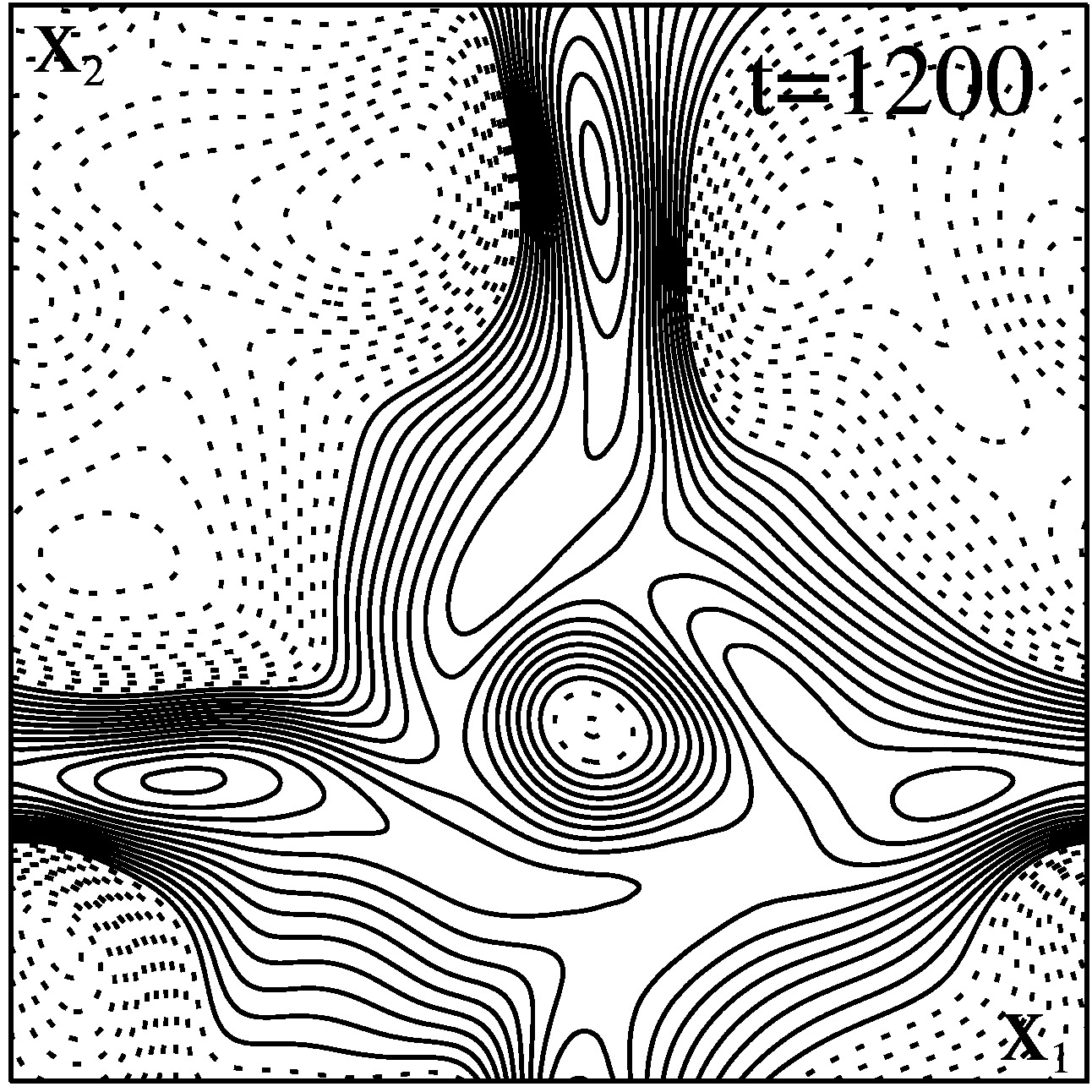
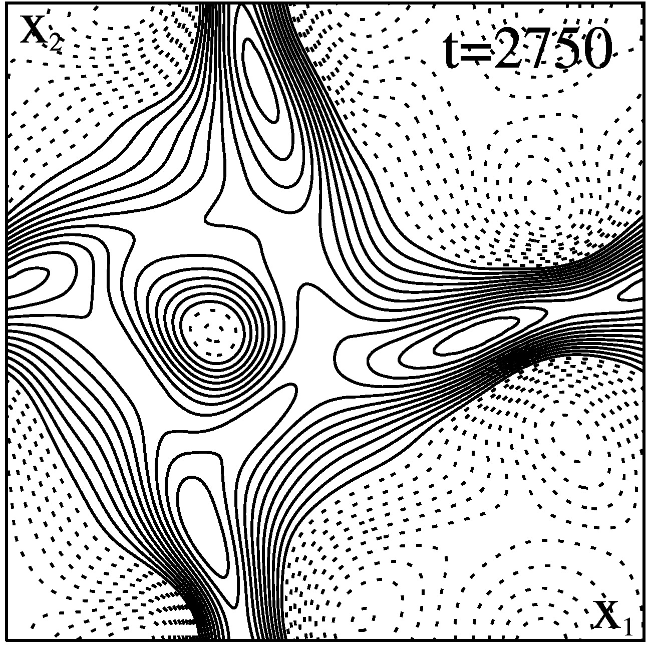
(a)                     (b)                     (c)

(d)                           (e)

Figure 4: Kinetic energy evolution, the Poincaré sections and the vertival velocity profiles for the intermittent attractor at Ra=2075. On the top and (a) panels the same as on fig. 2 is shown. Points from (a) for the trajectories intersecting the Poincaré plane for $400\leq{t}\leq 1900$ (b) and $2500\leq{t}\leq 3000$ (c). Four open circles in (c) show where the stable periodic orbit for Ra=2055 from branch $\rm{A}_{2}$ intersects the Poincaré plane. Isolines of $v_{3}$ on the horizontal mid-plane $x_{3}=1/2$ are shown for $t=1200$ (d) and $t=2750$ (e) (solid and dashed lines stand for positive and negative values, respectively).

For $2073\leq{\rm Ra}\leq 2080$, the family B₁ gives rise to an attractor (B₂) displaying “in-out” intermittent behaviour [29], i.e., the trajectory switches irregularly in time between two main states, one is a time-periodic state corresponding to the destabilized ${\rm A}_{2}$, the other is chaotic, corresponding to the destabilized ${\rm B}_{1}$. Fig. 4 shows the time series, Poincaré sections and velocity profiles for the attractor at Ra=2075; the trajectory in the phase space visits the periodic state at $0\leq{t}\leq 200$ and $2100\leq{t}\leq 3200$. Thus, B₂ is formed by a crisis-like event involving the previously destabilized A₂ and B₁. However, a comparison between the right panel of fig. 3 (j) and fig. 4 (a) reveals that B₂ is larger than the union of A₂ and B₁. The missing component can be found from a set of initial conditions displaying chaotic transients for ${\rm Ra}<2073$. This set constitutes a chaotic saddle (CS), i.e., a nonattracting chaotic set responsible for chaotic transients [30, 31]. Figs. 5(a) and (b) reveal the kinetic energy time series of two initial conditions at Ra=2070. Both trajectories exhibit chaotic behavior for about 100 time units, before they escape from the chaotic region toward the destabilized A₂. Later, the same trajectories will converge to attractor B₁. The Poincaré plot for the union of the transient parts of both series is shown on fig. 5 (c) and resembles the Poincaré plots of figs. 4 (b) and (c). From all this information, we conjecture the following scenario. Attractor A₂ is destabilized in a boundary crisis at Ra$\approx$2055 after a collision with CS, a chaotic saddle lying on the basin boundary between A₂ and B₁. The unstable set formed by the union of CS and the destabilized A₂, then, collides with B₁ at an interior crisis at Ra$\approx$2073 (IC1 in fig. 1), leading to the intermittent attractor B₂, where trajectories alternate between phases where A₂, CS and B₁ can be identified. The highest energy bursts in fig. 4 correspond to CS.

On increasing Ra, the intermittent attractor loses its stability, and trajectories for $2090\leq{\rm Ra}\leq 2130$ are attracted to A₃. However, chaotic transients reminiscent of the intermittent attractor B₂ remain all throughout this interval as a signature of a chaotic saddle in the background of A₃. For ${\rm Ra}\geq 2140$, the stability of A₃ is lost, and a new chaotic attractor, B₃, rises as (apparently) the sole attractor in the system. This attractor resembles B₂ and the chaotic saddle (cf. the kinetic energy evolution for Ra=2075 from B₂ in fig. 4, and for Ra=2140 and Ra=2200 from B₃ in fig. 6). In the intermittent regimes of B₃, the time spent near a state with regular behaviour is shortening for increasing Ra (cf.regimes at Ra=2140, top panel of fig. 6, and at Ra=2200, bottom panel of fig. 6). Note that some of the regular phases of the intermittency are in the region previously occupied by A₃. This corroborates another interior crisis scenario (IC2 in fig 1), whereby attractor A₃ collides with the background chaotic saddle to form an enlarged chaotic attractor B₃, where intermittent switches between the former A₃ and the chaotic saddle take place. Such crisis-induced intermittency involving a destabilized attractor and a surrounding chaotic saddle was reported for a one-dimensional spatiotemporally chaotic system in [32].

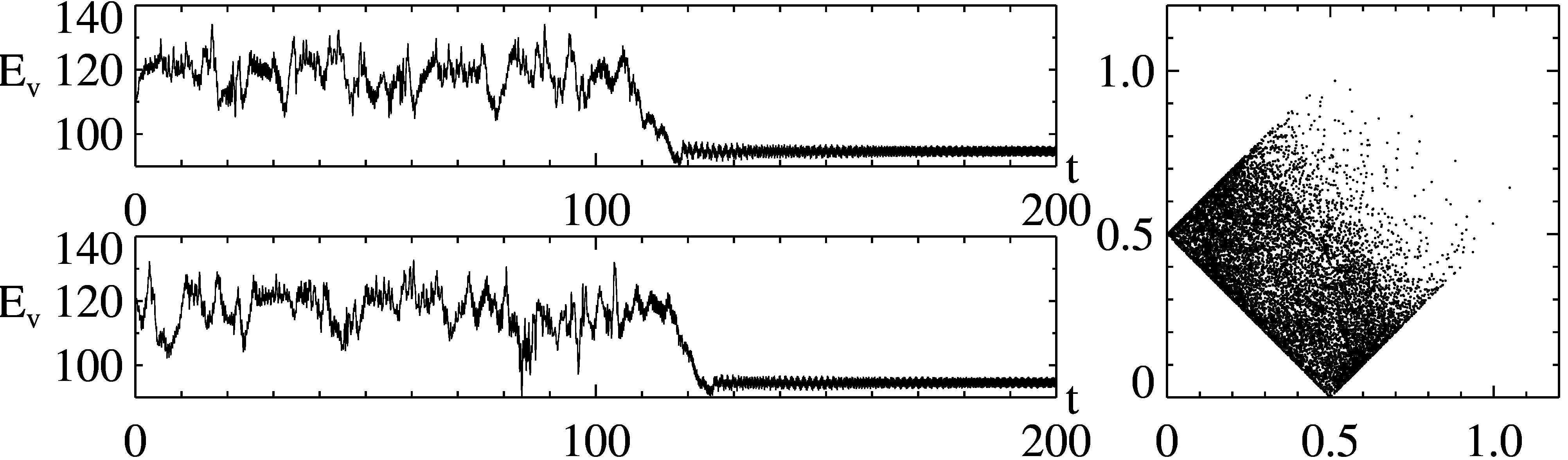
(a)       (c)

(b)

Figure 5: Kinetic energy evolution of transients for Ra=2070 ((a) and (b)) and Poincaré section for the transients (c). These transients are in the vicinity of a chaotic saddle in the phase space. The axes are as in fig. 2.

Figure 6: Kinetic energy evolution for the attractors of the family B₃ for Ra=2140 (top panel) and Ra=2200 (bottom panel).

The three largest Lyapunov exponents for the attractors from branches B₁ and B₃ of fig. 1 are shown in fig. 7 as a function of Ra. Hyperchaos with at least three positive Lyapunov exponents is observed after the interior crisis of B₃. Note the linear scaling of the exponents with Ra, a feature that has been observed in Rayleigh-Bénard convection near the onset for the first exponent as a function of the reduced Rayleigh number by [33]. The gap between B₁ and B₃ is filled by a chaotic saddle that evolves from the destabilized B₁. Although we have not computed the Lyapunov exponents of the chaotic saddle due to its repelling nature, we believe it should show a continuation of the linear scaling observed in fig. 7.

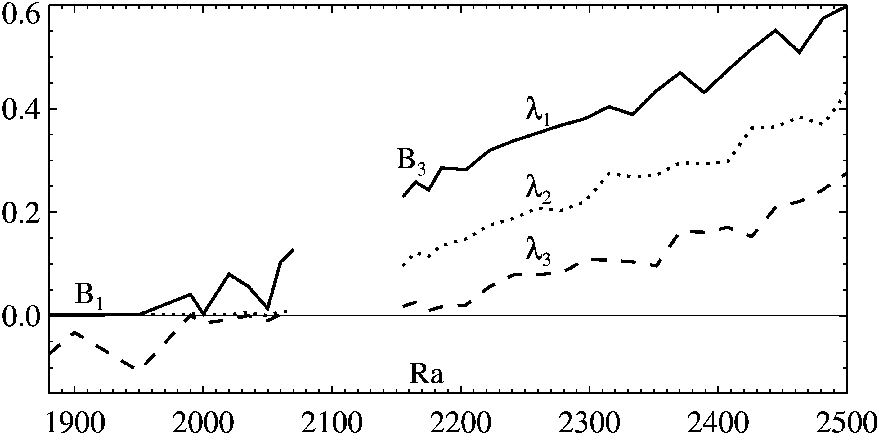
Figure 7: The three largest Lyapunov exponents (vertical axis) for the attractors of the families B₁ and B₃.

4 Conclusions

We have shown that the evolution from periodic convective states to hyperchaos in Rayleigh-Bénard convection for $P=0.3$ occurs through a sequence of local and global bifurcations as the Rayleigh number is increased, including three crises. First, a quasiperiodic attractor A₂ coexisting with another attractor B₁ collides with a chaotic saddle (CS) in the basin boundary and loses stability due to a boundary crisis. Evidence for this is based on A₂ becoming transient and the disappearance of its basin of attraction. Then, the newly formed chaotic saddle (CS + destabilized A₂) collides with the chaotic attractor B₁ in an interior crisis (IC1) leading to an enlarged attractor B₂. The evidence is the intermittent switching between B₁, CS and A₂. Next, attractor B₂ is destabilized and generates a chaotic saddle surrounding a quasiperiodic attractor A₃ (evidenced by B₂ becoming transient and the destruction of its basin of attraction). Finally, A₃ collides with the surrounding chaotic saddle in another interior crisis (IC2), which is evident from the intermittent switching between A₃ and CS in the time series. The enlarged attractor B₃ exhibits hyperchaos with at least three positive Lyapunov exponents.

Although strictly speaking a crisis is a collision of a chaotic attractor with a saddle invariant set [34], in a more general definition, a crisis can be described as a collision between any attractor and a saddle-type invariant set [35]. In the present letter, two of the identified crises involve the collision of a quasiperiodic attractor and a chaotic saddle.

There is surprising similarity between our results and the route to chaos found in [22], where two-dimensional Rayleigh-Bénard convection was studied for $P=6.8$. However, the attractors found ibid. are of a limited interest in hydrodynamics, because two-dimensional convective flows for the considered value of $P$ are stable only in a narrow window of parameter values [16, 17]. They are also not useful in the dynamo theory, since magnetic field generation by a planar flow is impossible by virtue of the Zeldovich antidynamo theorem (see [1] for details). Note that our results also have some correlation with the bifurcation diagram shown in [36] for zero Prandtl number near the onset of convection, where stationary, oscilating and chaotic regimes are found, although no hyperchaos was reported then, probably due to the low values of Ra. Intermittent and chaotic waves were also found in [37] for $P=0.2$ as well as $P=0$, with both free-slip and no-slip boundary conditions for small aspect ratio geometries.

Experimental verification of some bifurcations reported here have been found in the past for Rayleigh-Bénard convection, such as abrupt transitions from quasiperiodic to chaotic attractors [38], a route to chaos via intermittency [39], and quasiperiodic attractors with three basic frequencies [40].

Regarding future works, note that we have not fully characterised all bifurcations presented and, in particular, the destabilisation of B₂ (supposedly another boundary crisis) was not investigated. Additionally, we do not claim to have found all the attractors present in the range of Ra studied. Continuing the line of research started in [11, 41, 42], we plan to add rotation and magnetic field, whereby one can study mechanisms of the convective electromagnetic processes in the liquid outer core of the Earth.

RC and ELR acknowledge financial support from FAPESP (Brazil, grants 2013/01242-8 and 2013/22314-7, respectively). ELR also acknowledges financial support from CNPq (Brazil, grant 305540/2014-9). EVC acknowledges financial support from CAPES.

References

- [1] \NameMoffat H. \BookMagnetic Field Generation in Electrically Conducting Fluids (Cambridge University Press) 1978.
- [2] \NameOssendrijver M. \REVIEWAstron. Astrophys. Rev.112003287.
- [3] \NameSchubert G., Turcotte D. Olson P. \BookMantle Convection in the Earth and Planets (Cambridge University Press) 2001.
- [4] \NameOlson P. \BookOverview in \BookTreatise on Geophysics, Volume 8: Core Dynamics, edited by \NameSchubert G. (Elsevier) 2007 pp. 1–30.
- [5] \NameFearn D. Roberts P. \BookThe geodynamo (Roca Baton: CRC Press) 2007.
- [6] \NameJones C. A. \REVIEWAnnu. Rev. Fluid Mech.432011583.
- [7] \NameGubbins D. \REVIEWPhys. Earth Planet. Inter.12820013.
- [8] \NameCalkins M. A., Aurnou J. M., Eldredge J. D. Julien K. \REVIEWEarth Planet. Sci. Lett.359–360201255 .
- [9] \NameŠoltis T. Šimkanin J. \REVIEWContributions to Geophysics and Geodesy442014293.
- [10] \NameBusse F. \REVIEWAnnu. Rev. Fluid Mech.322000383.
- [11] \NamePodvigina O. M. \REVIEWGeophys. Astrophys. Fluid Dyn.1022008409.
- [12] \NameBodenschatz E., Pesch W. Ahlers G. \REVIEWAnnu. Rev. Fluid Mech.322000709.
- [13] \NameCross M. C. Hohenberg P. \REVIEWRev. Mod. Phys.651993851.
- [14] \NameChandrasekhar S. \BookHydrodynamic and Hydromagnetic Stability (Dover Publications) 1961.
- [15] \NameGetling A. \BookRayleigh-Bénard Convection: Structures and Dynamics (World Scientific) 1998.
- [16] \NameBusse F. H. Bolton E. W. \REVIEWJ. Fluid Mech.1461984115.
- [17] \NameBolton E. W. Busse F. H. \REVIEWJ. Fluid Mech.1501985487.
- [18] \NameMeneguzzi M., Sulem C., Sulem P. L. Thual O. \REVIEWJ. Fluid Mech.1821987169.
- [19] \NameBorońska K. Tuckerman L. \REVIEWPhys. Rev. E812010036321.
- [20] \NameEgolf D., Melnikov I., Pesch W. Ecke R. \REVIEWNature4042000733.
- [21] \NameKarimi A. Paul M. \REVIEWPhys. Rev. E852012046201.
- [22] \NamePaul S., Wahi P. Verma M. K. \REVIEWInt. J. Nonlinear. Mech.462011772 .
- [23] \NameManneville P. \BookRayleigh-Bénard convection: thirty years of experimental, theoretical, and modeling work in \BookDynamics of spatio-temporal cellular structures, edited by \NameMutabazi I., Wesfreid J. E. Guyon E. (Springer) 2006 pp. 41–65.
- [24] \NameCanuto C., Hussaini M., Quarteroni A. Zang T. \BookSpectral Methods: Fundamentals in Single Domains (Springer) 2006.
- [25] \NameCox S. M. Matthews P. C. \REVIEWJ. Comput. Phys.1762002430.
- [26] \NameHramov A. E., Koronovskii A. A., Maximenko V. A. Moskalenko O. I. \REVIEWPhys. Plasmas192012082302.
- [27] \NameOtt E. \BookChaos in Dynamical Systems (Cambridge University Press) 2002.
- [28] \NameChossat P. Lauterbach R. \BookMethods in Equivariant Bifurcations and Dynamical Systems (World Scientific) 2000.
- [29] \NameCovas E., Tavakol R., Ashwin P., Tworkowski A. Brooke J. \REVIEWChaos112001404.
- [30] \NameHsu G.-H., Ott E. Grebogi C. \REVIEWPhys. Lett. A1271988199.
- [31] \NameRempel E. L., Chian A. C.-L., Macau E. E. N. Rosa R. R. \REVIEWPhysica D1992004407.
- [32] \NameRempel E. L. Chian A. C.-L. \REVIEWPhys. Rev. Lett.982007014101.
- [33] \NameJayaraman A., Scheel J. D., Greenside H. S. Fischer P. F. \REVIEWPhys. Rev. E742006016209.
- [34] \NameGrebogi C., Ott E., Romeiras F. Yorke J. A. \REVIEWPhys. Rev. A3619875365.
- [35] \NameWitt A., Feudel F. Pikovsky A. \REVIEWPhysica D1091997180.
- [36] \NamePal P., Wahi P., Paul S., Verma M. K., Kumar K. Mishra P. K. \REVIEWEurophys. Lett.87200954003.
- [37] \NameThual O. \REVIEWJ. Fluid Mech.2401992229.
- [38] \NameSwinney H. Gollub J. \REVIEWPhysics Today31197841.
- [39] \NameBergé P., Dubois M., Mannevillel P. Pomeau Y. \REVIEWJournal de Physique Lettres411980341.
- [40] \NameGollub J. Benson S. \REVIEWJ. Fluid Mech.1001980449.
- [41] \NameChertovskih R., Gama S., Podvigina O. Zheligovsky V. \REVIEWPhysica D23920101188.
- [42] \NamePodvigina O. \REVIEWEur. Phys. J. B502006639.