A possible geometrical origin of the accelerated expansion of the universe

Abstract

The modified geodetic brane cosmology (MGBC) is tested with observational data. The MGBC is derived from the geodetic brane gravity action corrected by the extrinsic curvature of the braneworld. The density parameter coming from this additional term produces an accelerated expansion of geometrical origin. Subject to the Supernovae Ia, Observable Hubble parameter, Baryon Acoustic Oscillations and Cosmic Microwave Background probes, the obtained fit provides enough evidence in the sense that the extrinsic curvature effect is able to reproduce the accelerated expansion of the universe without need of invoking dark energy, exotic matter or cosmological constant. Moreover the MGBC is free of the problems present in other braneworld models.

I Introduction

One of the current challenging problems in physics is the explanation of the accelerated expansion of the Universe. The main hypothesis to explain this fact relies on the existence of an unusual energy form, the so-called dark energy, that for example can be produced by scalar fields incarnated in a great variety of field theories like quintessence, k-essence, Galileons, etc Amendola and Tsujikawa (2010). Aside, a plenty of modified theories of gravity have been proposed to elucidate the origin of the cosmic acceleration like $f(R)$ gravity, scalar-tensor theories, braneworlds models, etc. Regarding this last, in the past decade an intense research on the braneworld models has captivated cosmologists Arkani-Hamed et al. (1998); Antoniadis et al. (1998); Randall and Sundrum (1999a, b); Dvali et al. (2000). Some of these models do have an accelerated epoch where exotic matter is not needed.

An attempt tied only to geometry to model our accelerated Universe was suggested recently and named modified geodetic brane cosmology Cordero et al. (2012) (MGBC), based in the RT model  Regge and Teiltelboim (1977); Davidson and Karasik (1998); Karasik and Davidson (2003). This turns out to be an alternative to the cosmological constant problem for describing the late accelerated expansion of the Universe. It can also be thought as an implementation of a gravity theory from the perspective of string theory. In this framework gravity, through a Ricci scalar, is considered to be induced on a hypersurface which is evolving in a higher dimensional Minkowski space besides of taking into account a linear correction term in the extrinsic curvature of the brane trajectory. Physically, this correction term can be considered as a remanent of the Dvali, Gabadadze and Porrati (DGP) Dvali et al. (2000) model that modifies General Relativity (GR) and exhibiting a self-accelerated phase that may explain the current cosmological expansion. In this sense, MGBC mimics the accelerating expansion of this type of universe.

There is a main difference with general relativity. Unlike usual gravity theories where the metric components are considered to be fundamental variables, in MGBC the embedding functions are the field variables instead of the four-dimensional metric components. Within a minisuperspace framework these local coordinates induced on the hypersurface are considered to be dynamical and form a minisuperspace in the higher dimensional embedding space. This type of model is often called geodetic brane gravity (GBG) Davidson and Karasik (1998) since it is not considered the gravitational effect of the brane on the background spacetime. In fact, since the point of view of the so called unified brane cosmology (UBC) discussed by Davidson and Gurwich Gurwich and Davidson (2009), the GBG is one part of several brane models like Randall-Sundrum (RS) Randall and Sundrum (1999a, b), DGP and RT models that can be described in a unified way. In the unified brane cosmology, by means of a Dirac brane style variation, the effect of gravity produced by the brane in the bulk is considered and the Israel Junction conditions are relaxed. If the gravitational effect of the brane on the bulk is not considered the equations of motion can be obtained by taking the background gravitational constant very large. A fundamental quantity that enters into the game is the conserved bulk energy and plays the role of a parameter that deviates the model from GR.

On geometrical grounds, the MGBC is conformed only by the first three Lovelock brane invariants associated to the brane trajectory (our Universe). Such second-order field theories are conformed by actions whose Lagrangian is the sum of geometric quantities constructed from the extrinsic curvature and the induced metric

$$L =a_{0}+a_{1}K+a_{2}R+a_{3}(K^{3}-3KK_{\mu\nu}K^{\mu\nu}+2K^{\mu}_{\alpha}K^{\alpha}_{\beta}K^{\beta}_{\mu})$$

$$+a_{4}(R^{2}-4R_{\mu\nu}R^{\mu\nu}+R_{\alpha\beta\gamma\delta}R^{\alpha\beta\gamma\delta})+a_{5}{\cal O}(K^{5}),$$ (1)

where $R$, $R_{\mu\nu}$ and $R_{\mu\nu\alpha\beta}$ are the Ricci scalar, Ricci tensor and the Riemann tensor constructed by the associated Gauss-Codazzi integrability condition for surfaces, $R_{\mu\nu\alpha\beta}=K_{\mu\alpha}K_{\nu\beta}-K_{\mu\beta}K_{\nu\alpha}$, and $K_{\mu\nu}$ is extrinsic curvature of the worldvolume, respectively Cruz and Rojas (2013). The ensuing equations of motion from (1) remain second-order which leads to a ghost-free field theory.

In spite of its theoretical predictions, MGBC has not been observationally tested. This is the purpose of the present paper. To make progress on this issue, we report here the results of probing the MGBC with Supernovae Ia (SNe Ia), direct observations of the Hubble parameter (OHD), Baryon Acoustic Oscillations (BAO) and Cosmic Microwave Background (CMB). The agreement is very promising that allow us to conclude that the current accelerated expansion might be of geometric origin. Moreover, based on these results, the idea that our $4D$ universe floats within a fifth dimension must not be ruled out yet. The inclusion of the $K$ term is not a simple improvisation. It has been considered in several contexts ranging from the bending and shape determination of phospholipids membranes Svetina and Zekz (1989), in particle physics models to improve the earlier attempt by Dirac to picture the electron as a bubble Onder and Tucker (1988); Cordero et al. (2011), in pure GR as being the well known Gibbons-Hawking-York term, and recently as an effective $4D$ field yielding one of the Galileon actions with applications in particle physics and cosmology de Rham and Tolley (2010); Goon et al. (2011).

The paper is organized as follows. In Section II we briefly review the MGBC and confine our attention to the expression for the Hubble parameter in terms of the matter density parameters, that will be used in the tests. In Section III the probes and statistical method are described. The results are discussed in Section IV and finally the concluding remarks are given in the last Section.

II The Modified Geodetic Brane Cosmology

Let us briefly review the MGBC model as well as the derivation of the Friedmann equations that are taken as the basis for the cosmological data confrontation. Detailed calculations can be found in Cordero et al. (2012). Consider a spacelike 3-brane $\Sigma$, propagating in a flat five-dimensional nondynamical Minkowski background spacetime with metric $\eta_{AB},\,(A,B=0,1,2,3,4)$. The brane trajectory or worldvolume, $m$, is an oriented timelike $4$-dimensional hypersurface parametrized by $y^{A}=X^{A}(x^{\mu})$ in the bulk where $y^{A}$ are the local coordinates for the background spacetime, and $x^{\mu}$ are the local coordinates for $m$ while $X^{A}$ are the embedding functions ($\mu=0,1,2,3$). In general, any 4 dimensional brane Universe can be embedded at least locally for a background spacetime with dimension $N\geq 10$ Janet (1926); Cartan (1927), and for $N\geq 91$ a global Clarke (1970) embedding is possible. In this spirit, a Friedmann-Robertson-Walker (FRW) metric can be embedded in a 5 dimensional background Rosen (1965).

The dynamics of $\Sigma$ under the MGBC model is derived from the functional

$$S[X]=\int_{m}d^{4}x\,\sqrt{-g}\left({\frac{\alpha}{2}{R}+\beta K-\Lambda}\right),$$ (2)

where the constants $\alpha$ and $\beta$ have the dimensions [L]^-2 and [L]^-3 in Planck units, respectively; $g={\rm det}(g_{\mu\nu})$, $R$ stands for the worldvolume Ricci scalar, $K=g^{\mu\nu}K_{\mu\nu}$ is the mean extrinsic curvature of $m$, and $\Lambda$ is the cosmological constant defined on $m$. The action (2) is invariant under reparametrizations of the worldvolume and it leads to an only second-order equation of motion.

From the action it is obtained the generalized geodetic equation that governs the $\Sigma$ evolution,

$$(\alpha G^{\mu\nu}+\beta S^{\mu\nu}+\Lambda g^{\mu\nu})K_{\mu\nu}=0,$$ (3)

where $G_{\mu\nu}=R_{\mu\nu}-Rg_{\mu\nu}/2$ is the worldvolume Einstein tensor and $S_{\mu\nu}:=K_{\mu\nu}-Kg_{\mu\nu}$. Notice that it is a second-order differential equation written in a compact form. The tensors $G_{\mu\nu},S_{\mu\nu}$ are conserved in the sense that $\nabla_{\mu}G^{\mu\nu}=0$ and $\nabla_{\mu}S^{\mu\nu}=0$ where $\nabla_{\mu}$ is the covariant derivative compatible with the induced metric $g_{\mu\nu}$ (see Cruz and Rojas (2013) for more details). We assume that the five-dimensional Minkowski spacetime, where $\Sigma$ evolves, is

$$ds_{5}^{2}=-dt^{2}+da^{2}+a^{2}d\Omega_{3}^{2},$$ (4)

where $d\Omega_{3}^{2}$ denotes the unit 3-sphere. In addition, by assuming that on large scales this type of universe is homogeneous and isotropic, the worldvolume $m$ can be parametrized by $y^{A}=X^{A}(\xi^{\mu})=(t(\tau),a(\tau),\chi,\theta,\phi))$, with $\tau$ being the proper time for an observer at rest w. r. t. the brane. This is the usual Friedmann-Robertson-Walker (FRW) geometry. Thus, the metric induced from the background spacetime is

$$ds_{4}^{2}=-N^{2}dt^{2}+a^{2}d\Omega_{3}^{2}=g_{\mu\nu}dx^{\mu}dx^{\nu}.$$ (5)

where $N=\sqrt{\dot{t}^{2}-\dot{a}^{2}}$. The evolution of the brane $\Sigma$, derived from Eq. (3) under the FRW geometry is given by

$$\frac{d}{d\tau}\left({\frac{\dot{a}}{\dot{t}}}\right)=-\frac{N^{2}}{a^{2}(\dot{t}/a)}\frac{(\dot{t}^{2}/a^{2}-3\bar{\Lambda}N^{2}+6\bar{\beta}N\dot{t}/a)}{(3\dot{t}^{2}/a^{2}-\bar{\Lambda}N^{2}+6\bar{\beta}N\dot{t}/a)},$$ (6)

where $\bar{x}$ denotes $x/(3\alpha)$ and $\dot{x}$ means derivative w. r. t. the parameter $\tau$. Later on it will be clear that depending on its sign, the $\beta$ parameter contributes as either a catalyst or a preventer of the acceleration of this type of universe.

So far this review comprises only the geometrical information. If we intend to make contact with the cosmological implications of the model we need to include the brane matter content which should be compatible with the assumed symmetries. Thus, a perfect fluid fulfills these requirements

$$T_{m}^{\mu\nu}=(\rho+P)\eta^{\mu}\eta^{\nu}+Pg^{\mu\nu},$$ (7)

where $\eta^{\mu}$ denotes the timelike unit normal vector to $\Sigma$, and $\rho(a)$ and $P(a)$ are the energy density and pressure of the fluid, respectively. It was also shown that since the model is invariant under reparametrizations in the time coordinate $t$, the energy $E$ of the brane trajectory of this brane-like universe results constant and given by

$$-\frac{E}{a^{4}}=\frac{(\dot{a}^{2}+k)^{1/2}}{a}\left[\frac{(\dot{a}^{2}+k)}{a^{2}}-(\overline{\Lambda}+\overline{\rho})\right]+3\overline{\beta}\frac{(\dot{a}^{2}+k)}{a^{2}},$$ (8)

where we have considered the three possible geometries for this type of universe through the parameter $k$ ($k=-1,0,1$) besides of considering the so-called cosmic gauge, $N=1$. Some remarks are in order. Expression (8) is nothing but the Friedmann equation associated to the model (2). It is noteworthy that $E$, being and integration constant, it parametrizes the deviation from the Einstein limit since as $E\to 0$ and $\beta\to 0$ together, the standard cosmology is recovered. Finally, notice that this is a peculiar algebraic cubic equation in the combination $(\dot{a}^{2}+k)^{1/2}/a$ such that it only possesses a single physical solution Cordero et al. (2012).

At this point it is important to remark the similarities and differences and between MGBC and UBC. The MGBC is one part of the UBC and it can be obtained if the gravitational effect of the brane on the bulk is not considered by means of taking the gravitational constant of the background spacetime very large (smooth background case). The term $\frac{E}{a^{4}}$ was introduced before the RS radiation term and its origin is different because in the later case this term comes once the FRW brane is embedded in a Schwarzchild-AdS₅ black hole background spacetime. Since the point of view of UBC (for $Z_{2}$ symmetry) $E$ parametrizes the deviation from General Relativity and RS model and it is not necessary small.

Inclusion of matter will not affect the form of the equation of motion (3). Hence, within this FRW geometry expression (3) in terms of the energy $E$ and in presence of a perfect fluid, reads

$$\frac{\ddot{a}}{a}=\frac{\left({\frac{\dot{t}^{2}}{a^{2}}}\right)\left[\frac{E}{a^{4}}-3\bar{\beta}\frac{\dot{t}^{2}}{a^{2}}+2(\bar{\Lambda}+\bar{\rho})\frac{\dot{t}}{a}-3(\bar{P}+\bar{\rho})\frac{\dot{t}}{a}\right]}{\left[-3\frac{E}{a^{4}}-3\bar{\beta}\frac{\dot{t}^{2}}{a^{2}}+2(\bar{\Lambda}+\bar{\rho})\frac{\dot{t}}{a}\right]}.$$ (9)

A convenient form to rewritting the Friedmann equation (8) is in terms of the Hubble parameter $H:=\dot{a}/a$ as well as the energy density parameters associated with the model. Thus, Eq. (8) becomes

$$\left({\frac{H^{2}}{H_{0}^{2}}-\frac{\Omega_{k,0}}{a^{2}}}\right)^{1/2}\left({\frac{H^{2}}{H_{0}^{2}}-\frac{\Omega_{k,0}}{a^{2}}-\frac{\Omega_{m,0}}{a^{3}}-\Omega_{\Lambda,0}}\right)+$$

$$\Omega_{\beta,0}\left({\frac{H^{2}}{H_{0}^{2}}-\frac{\Omega_{k,0}}{a^{2}}}\right)=\frac{\Omega_{dr}}{a^{4}},$$ (10)

where the density parameters are defined by $\Omega_{\Lambda,0}:=\Lambda/(3\alpha H_{0}^{2})$, $\Omega_{m,0}:=\rho_{m,0}/(3\alpha H_{0}^{2})$, $\Omega_{\beta,0}:=\beta/(\alpha H_{0})$ and the so called dark radiation density parameter $\Omega_{dr}:=-E/(H_{0}^{3})$. $H_{0}$ being the Hubble constant.

As it was pointed out in Cordero et al. (2014), the case when $\Omega_{dr}=0$ and $\beta>0$ corresponds to the non-accelerating branch of the DGP theory, whereas $\Omega_{dr}=0$ and $\beta<0$ conforms a self-accelerating branch similar to the one of the DGP framework, and therefore appears a number of pathologies. Notice also that the $\beta$ parameter plays the role of the inverse of the crossover scale $r_{c}$, related to the transition from $4D$ to $5D$ in the DGP approach. Furthermore, $\beta$ is related to the $5D$ Planck mass in the context of the Galileon field theory of brane cosmology de Rham and Tolley (2010). The normalization condition is obtained by evaluating Eq. (10) at the present moment,

$$\left({1-\Omega_{k,0}}\right)^{1/2}\left({1-\Omega_{k,0}-\Omega_{m,0}-\Omega_{\Lambda,0}}\right)+\Omega_{\beta,0}\left({1-\Omega_{k,0}}\right)=\Omega_{dr}.$$ (11)

As before, when $\Omega_{dr}=0$ and $\Omega_{\beta,0}=0$ the standard cosmology is recovered, accordingly. The general behaviour of the scale factor is studied in detail in Cordero et al. (2012). Now, (10) is an algebraic cubic equation in $H^{2}/H_{0}^{2}$ whose real root has been determined. This shall be used to compare with the cosmological data in the next Section. For sake of illustration, in the analysis below we shall assume a flat FRW type universe, i.e., by considering $\Omega_{k,0}=0$

III Statistics and Observational Samples

III.1 Statistical Method

To find the high confidence region of the parameter space of the MGBC given a set of observational data, we use the Markov Chain Monte Carlo (MCMC) method, which is an algorithm with the capability of providing robust and realistic constraints on cosmological model parameters. The method is fairly standard but suffers of an important complication consisting in how to approach correctly the convergence of the chain. In particular, our code addresses this issue following the prescription developed in Dunkley et al. (2005). See Berg (2004); MacKay (2003); Neal (1993) and references therein, for a review of MCMC methods.

By using our MCMC code, we perform a likelihood analysis in which we minimize the $\chi^{2}$ function thus obtaining the best fit of model parameters from observational data. This minimization is equivalent to maximizing the likelihood function $\mathcal{L}(\theta)\propto\exp[-\chi^{2}(\theta)/2]$ where $\theta$ is the vector of model parameters. The expression for $\chi^{2}(\theta)$ depends on the used dataset. In what follows we briefly describe the probes and samples.

III.2 Type Ia Supernovae (SNe Ia)

We consider the Union2.1 compilation of 580 SNe Ia in the redshift range $0.015<z<1.414$ reported by the Supernova Cosmology Project (SCP) Suzuki et al. (2012). As is usual, the comparison with SNe Ia data is made via the standard $\chi^{2}$ statistics given by

$$\chi^{2}_{SNeIa}=\mathrm{\Delta}\mathrm{\mu}\cdot\mathrm{C^{-1}}\cdot\mathrm{\Delta}\mathrm{\mu},$$ (12)

where $\mathrm{C}$ is the covariance matrix and $\mathrm{\Delta}\mathrm{\mu}=\mathrm{\mu_{th}}-\mathrm{\mu_{obs}}$ is the vector of the differences between the observed and theoretical value of the distance modulus $\mathrm{\mu}$. For Union2.1, $\mathrm{C}$ captures all identified systematic errors besides to the statistic errors of the SNe Ia data and $\mathrm{\mu}$ is defined by

$$\mu(z,\theta)=5\log_{10}\left[d_{L}(z,\theta)\right]+\mu_{0},$$ (13)

where $d_{L}(z,\theta)$ is the dimensionless luminosity distance given by

$$d_{L}(z,\theta)=(1+z)\int_{0}^{z}\frac{dz^{\prime}}{E(z^{\prime},\theta)},$$ (14)

with $E(z,\theta)=H(z,\theta)/H_{0}$ the dimensionless Hubble function, $H_{0}$ the Hubble constant and $\theta$ the free parameters of the cosmological model.

In Eq. (13) $\mu_{0}$ is a nuisance parameter that depends on both the absolute magnitude of a fiducial SN Ia and the Hubble constant. Here, we marginalize the $\chi^{2}_{SNeIa}$ over $\mu_{0}$.

III.3 Observational Hubble Data (OHD)

The observational Hubble parameter $H(z)$ data provide a direct measurement of the Hubble parameter, instead of its integral like the SNe Ia or the Baryon Acoustic Oscillations (BAO) probes.

So far the main complication of the OHD data is the number of data points available in comparison with SNe Ia luminosity distance data. However, we think the OHD data can help break the parameter degeneracies and shed light on the cosmological scenarios that are being studied.

In this work, we use 18 data points from differential evolution of passively evolving early-type galaxies in the redshift range $0<z<1.75$ reported in Moresco et al. (2012).

The best fit values of the model parameters from OHD are determined by minimizing the quantity

$$\chi^{2}_{OHD}=\sum^{18}_{j=1}\frac{\left[H_{th}(z_{j},\mathbf{\theta})-H_{obs}(z_{j})\right]^{2}}{\sigma^{2}_{H_{obs}}(z_{j})},$$ (15)

where $\sigma^{2}_{H_{obs}}$ are the measurement variances, and $\mathbf{\theta}$ corresponds to the free parameters of the cosmological model.

III.4 Baryon Acoustic Oscillations (BAO)

Currently BAO is considered a promising standard ruler to use in cosmology enabling precise measurements of the distance ratio, $D_{V}/r_{s}$, the distance to objects at redshift $z$ in units of the sound horizon at recombination, independently of the local Hubble constant. The observed angular and radial BAO scales at redshift $z$ provide a geometric estimate of the effective distance,

$$D_{V}(z)\equiv\left[(1+z)^{2}D_{A}^{2}(z)cz/H(z)\right]^{1/3},$$ (16)

where $D_{A}(z)$ is the angular diameter distance and $H(z)$ is the Hubble parameter. The measured ratio $D_{V}/r_{s}$, with $r_{s}$ being the comoving sound horizon scale at the end of the drag epoch, is what can be compared to theoretical predictions.

Since the release of the seven-year WMAP data, the acoustic scale measurement has been improved by the Sloan Digital Sky Survey (SDSS) and SDSS-III Baryon Oscillation Spectroscopic Survey (BOSS) galaxy surveys, and by the WiggleZ and 6dFGS surveys. An upgraded estimate of the acoustic scale in the SDSS-DR7 data was made in Padmanabhan et al. (2012), giving $D_{V}(0.35)/r_{s}=8.88\pm 0.17$, and reducing the uncertainty from 3.5$\%$ to 1.9$\%$. More recently, the SDSS-DR9 data from the BOSS survey has been used to estimate the BAO scale of the CMASS sample. In this last case, in Anderson et al. (2012) was reported $D_{V}(0.57)/r_{s}=13.67\pm 0.22$ for galaxies in the range $0.43<z<0.7$ (at an effective redshift $z=0.57$). On the other hand, the acoustic scale has also been measured at higher redshift using the WiggleZ galaxy survey. In Blake et al. (2012) was reported distances in three correlated redshift bins between $0.44$ and $0.73$. At lower redshift, $z=0.1$, a detection of the BAO scale has been made using the 6dFGS survey, see Beutler et al. (2011). To perform our analysis we employed the data described before; a summary of these measurements can be found in Table 1 of Hinshaw et al. (2013).

The corresponding $\chi^{2}$ is given by

$$\chi^{2}_{BAO}=(v_{i}-v_{i}^{BAO})(\mathbf{C}^{-1})_{ij}^{BAO}(v_{j}-v_{j}^{BAO})^{T},$$ (17)

where $(\mathbf{C}^{-1})^{BAO}$ is the inverse covariance matrix of the data and $v_{i}$ is given by $v_{i}=\left\{\frac{r_{s}(z_{drag};\mathbf{\theta})}{D_{V}(z;\theta)}\right\}$.

III.5 Cosmic Microwave Background (CMB)

We also use the CMB data reported in Wang and Wang (2013), where distance priors are derived from the first release of the Planck results.

CMB data provide the comoving distance to the photon-decopling surface $r(z_{*})$, $z_{*}=1090$, and the comoving sound horizon at photon-decopling epoch $r_{s}(z_{*})$ which are defined as,

$$r(z_{*})=\frac{c}{H_{0}}\int_{0}^{z_{*}}\frac{dz^{\prime}}{E(z^{\prime})},$$ (18)

and

$$r_{s}(z_{*}) = \frac{c}{H_{0}}\int_{z_{*}}^{\infty}\frac{c_{s}}{E(z^{\prime})}dz^{\prime}$$

$$\equiv \frac{c}{H_{0}}\int_{0}^{a_{*}}\frac{da^{\prime}}{\sqrt{3(1+\overline{R_{b}}a^{\prime})a^{\prime 4}E^{2}(a^{\prime})}},$$

where $\overline{R_{b}}a=3\rho_{b}/(4\rho_{\gamma})=31500\Omega_{b}h^{2}(T_{CMB}/2.7K)^{-4}a$.

The CMB shift parameters are

$$R\equiv\sqrt{\Omega_{m}H_{0}^{2}}\frac{r(z_{*})}{c},$$ (20)

$$l_{a}\equiv\pi\frac{r(z_{*})}{r_{s}(z_{*})},$$ (21)

and both are evaluated at photon-decoupling epoch $z_{*}$. The baryon density $\Omega_{b}h^{2}$ is also considered as shift parameter.

The mean values for these shift parameters as well as their standard deviations and normalized covariance matrix are taken from Wang and Wang (2013). Thus, the corresponding $\chi^{2}$ for the CMB is

$$\chi^{2}_{CMB}=(v_{i}-v_{i}^{CMB})(\mathbf{C}^{-1})_{ij}^{CMB}(v_{j}-v_{j}^{CMB})^{T},$$ (22)

where $(\mathbf{C}^{-1})^{CMB}$ is the inverse covariance matrix of the data and $v_{j}$ means the vector parameter $(\mathbf{v})_{j}$, $\mathbf{v}=(l_{a},R,\Omega_{b}h^{2})$.

IV Observational results

Table 1: Summary of the Modified GBG cosmological scenarios tested.

Case	Free Parameters	Assumptions
I	$\Omega_{\beta}$, $\Omega_{dr}$, $\Omega_{\Lambda}$	$\Omega_{m}=0.315$
II	$\Omega_{\beta}$, $\Omega_{dr}$, $\Omega_{m}$	$\Omega_{\Lambda}=0$
III	$\Omega_{\beta}$, $\Omega_{m}$, $\Omega_{\Lambda}$	$\Omega_{dr}=\Omega_{r}$
IV	$\Omega_{\beta}$, $\Omega_{m}$	$\Omega_{dr}=\Omega_{r}$, $\Omega_{\Lambda}=0$
V	$\Omega_{\beta}$, $\Omega_{dr}$	$\Omega_{m}=0.315$, $\Omega_{\Lambda}=0$

In this section we will discuss the results of probing the MGBC cosmology with the observational samples. Five cases will be considered, some of them being very promising in explaining the current accelerated expansion.

In Table 1, we present a summary of the cases analyzed. Case I has as free parameters $\Omega_{\beta}$, $\Omega_{dr}$ and $\Omega_{\Lambda}$; for this case it is assumed the matter density of the universe is $\Omega_{m}=0.315$ as the Planck’s results suggest Ade et al. (2014). Case II has $\Omega_{\beta}$, $\Omega_{dr}$ and $\Omega_{m}$ as free parameters and we consider $\Omega_{\Lambda}=0$. Case III consists in taking $\Omega_{\beta}$, $\Omega_{m}$, $\Omega_{\Lambda}$ as free parameters and $\Omega_{dr}$ corresponding to the radiation density, $\Omega_{r}$. Case IV has as free parameters just to $\Omega_{\beta}$, $\Omega_{m}$ and it is assumed that $\Omega_{dr}=\Omega_{r}$, $\Omega_{\Lambda}=0$. Case V consists in taking $\Omega_{\beta}$, $\Omega_{dr}$ as free parameters of the model with the assumptions of $\Omega_{m}=0.315$, $\Omega_{\Lambda}=0$.

Table 2: Summary of the best estimates of model parameters for the Case I as well as for the best values for the parameter $\Omega_{\Lambda}$ coming from the normalization condition, Eq. (11) with $\Omega_{k,0}=0$. The errors are at $68.3\%$ confidence level. Here, to obtain the best estimates of model parameters, it has been assumed a prior on $\Omega_{m}=0.315\pm 0.012$ from the first Planck results Ade et al. (2014).

	SNIa	OHD	Joint
$\Omega_{\beta}$	$-0.074^{+0.191}_{-0.254}$	$-0.136^{+0.347}_{-0.473}$	$-0.084^{+0.204}_{-0.276}$
$\Omega_{dr}$	$0.028^{+0.031}_{-0.028}$	$0.038^{+0.068}_{-0.038}$	$0.023^{+0.038}_{-0.023}$
$\chi^{2}_{r}$	0.959	0.989	0.952
$\Omega_{\Lambda}$	$0.580^{+0.163}_{-0.223}$	$0.507^{+0.283}_{-0.431}$	$0.577^{+0.168}_{-0.252}$

Firstly we will describe the results obtained with SNIa and OHD data, while in the next subsection the BAO and CMB probes will be incorporated to the analysis.

The best fit parameter values with 1$\sigma$ error and the corresponding values of $\chi^{2}$ obtained by using SNIa data, OHD data and the joint of these data sets are summarized case by case in Tables 2 to 6.

Table 2 shows the results for the Case I. In this scenario the preferred amounts for $\Omega_{\beta}$ and $\Omega_{dr}$ from both data sets, SNIa data and OHD data, are very small; however by combining these data sets, the best-fit parameter values increase but not significantly. This results suggest that $\Omega_{\Lambda}$, although smaller than the one in $\Lambda$CDM, has to be present in order to drive the accelerated expansion.

For the Case II, the best-fit for $\Omega_{\beta}$ resulted to be as the MGBC model dictates in order to produce the cosmic acceleration, a negative quantity. Furthermore, $\Omega_{\beta}$ contributes in a significantly way. However from the normalization condition, Eq. (11), it is found that the amount of matter, $\Omega_{m}$, is inconsistent with the result given by Planck’s Ade et al. (2014), see Table 3. This case is therefore ruled out for explaining the accelerated expansion.

Table 3: Best estimates of model parameters for the Case II as well as for the best values for the parameter $\Omega_{m}$ from the normalization condition. The errors are at $68.3\%$ confidence level.

	SNIa	OHD	Joint
$\Omega_{\beta}$	$-0.808^{+0.056}_{-0.077}$	$-0.745^{+0.050}_{-0.073}$	$-0.779^{+0.046}_{-0.055}$
$\Omega_{dr}$	$0.089^{+0.127}_{-0.089}$	$0.127^{+0.163}_{-0.127}$	$0.103^{+0.131}_{-0.103}$
$\chi^{2}_{r}$	0.955	0.986	0.951
$\Omega_{m}$	$0.099^{+0.149}_{-0.099}$	$0.125^{+0.177}_{-0.125}$	$0.116^{+0.149}_{-0.116}$

Table 4 summarizes the results for the Case III. For this scenario, assuming $\Omega_{dr}$ equal to $\Omega_{r}$, the obtained best-fit value for $\Omega_{\beta}$ is almost negligible, meaning that the model cannot explain the accelerated expansion through this parameter, and instead $\Omega_{\Lambda}$ dominates the Universe in almost the same quantity dictated by the $\Lambda$CDM model.

Table 5 shows the observational constraints for the Case IV. It is assumed $\Omega_{\Lambda}=0$ and $\Omega_{dr}=\Omega_{r}$. The results coming from the OHD data, the SNIa data and the combination of the two samples point out that $\Omega_{\beta}$ could be responsible of cosmic acceleration. On the other hand, from the normalization condition is found that the matter content is smaller than the accepted value.

Table 4: Summary of the best estimates of model parameters for Case III as well as the best values for the parameter $\Omega_{\Lambda}$ obtained by the normalization condition. The errors are at $68.3\%$ confidence level. To obtain the best estimates it has been assumed $\Omega_{dr}=\Omega_{r}=\Omega_{\gamma}(1+0.2271N_{eff})$.

	SNIa	OHD	Joint
$\Omega_{\beta}$	$0.028^{+0.759}_{-0.869}$	$0.007^{+0.793}_{-0.791}$	$0.073^{+0.703}_{-0.868}$
$\Omega_{m}$	$0.300^{+0.174}_{-0.145}$	$0.343^{+0.145}_{-0.131}$	$0.331^{+0.133}_{-0.128}$
$\chi^{2}_{r}$	0.955	0.831	0.949
$\Omega_{\Lambda}$	$0.722^{+0.593}_{-0.722}$	$0.661^{+0.654}_{-0.661}$	$0.740^{+0.575}_{-0.740}$

Table 5: Best estimates of model parameters for Case IV as well as the best values for the parameter $\Omega_{m}$ obtained from the normalization condition. The errors are at $68.3\%$ confidence level. To obtain the best estimates it has been assumed $\Omega_{dr}=\Omega_{r}=\Omega_{\gamma}(1+0.2271N_{eff})$.

	SNIa	OHD	Joint
$\Omega_{\beta}$	$-0.797^{+0.037}_{-0.031}$	$-0.742^{+0.047}_{-0.048}$	$-0.768^{+0.035}_{-0.035}$
$\chi^{2}_{r}$	0.953	0.833	0.948
$\Omega_{m}$	$0.203^{+0.037}_{-0.031}$	$0.258^{+0.047}_{-0.048}$	$0.232^{+0.035}_{-0.035}$

Finally, Table 6 shows the results for the scenario (Case V) in which $\Omega_{\Lambda}=0$ and $\Omega_{m}=0.315$. The free parameter of the model is $\Omega_{\beta}$, and from the normalization condition straightforwardly is inferred $\Omega_{dr}$. In this case pretty good restrictions are obtained. The amount predicted for $\Omega_{\beta}$ is negative and very close to the abundance ascribed to $\Omega_{\Lambda}$. Taking together SNIa and OHD data we obtained as best-fit model parameter $\Omega_{\beta}=-0.679^{+0.002}_{-0.006}$ and $\Omega_{dr}=0.007^{+0.003}_{-0.007}$, from the normalization condition. As far as these probes concern, this is a good candidate to account for the observed accelerated expansion.

Table 6: Summary of the best estimates of model parameters as well as for the best values for the parameter $\Omega_{dr}$. The errors are at $68.3\%$ confidence level. In this case $\Omega_{\Lambda}=0$ and $\Omega_{m}=0.315$ (Case V).

	SNIa	OHD	Joint
$\Omega_{\beta}$	$-0.673^{+0.005}_{-0.012}$	$-0.673^{+0.008}_{-0.012}$	$-0.679^{+0.002}_{-0.006}$
$\chi^{2}_{r}$	0.972	1.069	0.969
$\Omega_{dr}$	$0.012^{+0.005}_{-0.012}$	$0.012^{+0.008}_{-0.012}$	$0.007^{+0.003}_{-0.007}$

IV.1 Complementing with BAO and CMB probes

Up to now we have performed observational tests by using SNIa and H(z) data, thus we have only focused on low-redshift probes. To arrive to more robust conclusions it is worth to study the MGBC model at high redshifts. In order to do that, we add a term of standard radiation, $\Omega_{r}$, in the Hubble parameter equation, Eq. (10), then the model becomes suitable to be confronted with BAO and CMB. BAO data is considered a powerful probe of dark energy and in turn, CMB data provide the strongest constraints on cosmological parameters thus being capable to break degeneracies between dark energy and cosmological parameters.

In Table 7 we present the results of the inclusion of these data sets. The constraints were derived from the union of all the observational data sets: SNIa, $H(z)$, BAO and CMB; in all cases we assume $\Omega_{r}=\Omega_{\gamma}(1+0.2271N_{eff})$ from the Planck results. By comparing the new results with the previous ones (SNIa and $H(z)$ data), we found a good agreement between them, thus validating our earlier conclusions. Notice that an important difference with this inclusion is that tighter constraints are obtained, which are easily observed in the errors of the cosmological parameters.

Table 7: Summary of the best estimates of model parameters obtained by the joint of SNIa, $H(z)$, BAO and CMB data for all the scenarios studied before. Separated of the former by a horizontal line are the parameters obtained from their respective normalization condition, $\Omega_{\Lambda}=0$, prior means $\Omega_{m}=0.315$ was assumed. For Cases III and IV, $\Omega_{dr}=\Omega_{r}$. The errors are at $68.3\%$ confidence level.

	Case I	Case II	Case III	Case IV	Case V
$\Omega_{\beta}$	$-0.023^{+0.035}_{-0.063}$	$-0.759\pm 0.004$	$-0.119^{+0.097}_{-0.099}$	$-0.759\pm 0.004$	$-0.6848\pm 0.0001$
$\Omega_{dr}$	$0.002^{+0.004}_{-0.002}$	$0.0004^{+0.0001}_{-0.0004}$	–	–	–
$\Omega_{m}$	–	–	$0.304\pm 0.012$	–	–
$\chi^{2}_{r}$	0.946	1.118	0.943	1.119	1.853
$\Omega_{\Lambda}$	$0.660^{+0.032}_{-0.060}$	0	$0.577^{+0.087}_{-0.089}$	0	0
$\Omega_{m}$	prior	$0.241^{+0.005}_{-0.003}$	–	$0.241\pm 0.004$	prior
$\Omega_{dr}$	–	–	$\Omega_{r}$	$\Omega_{r}$	$(8.9^{+3.5}_{-8.9})\times 10^{-5}$

In Figure 1, results are shown for Cases I and II; both panels show contours in the $\Omega_{\beta}$-$\Omega_{dr}$ parameter space. On the other hand, Figure 2 shows the constraints on the free parameters ($\Omega_{m}$ , $\Omega_{\beta}$) for the third scenario. In both figures 68$\%$ and 95$\%$ confidence level contours are displayed.

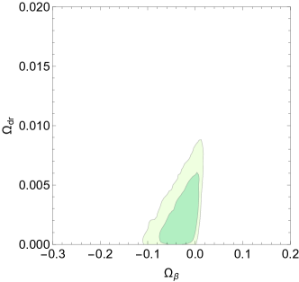
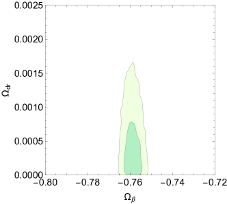
Figure 1: 1$\sigma$ and 2$\sigma$ contours in the $\Omega_{\beta}$-$\Omega_{dr}$ parameter space. Contours from the joint of SNIa, $H(z)$, BAO and CMB data. CASE I (Top Panel): It has been considered a prior on $\Omega_{m}$ from the Planck results Ade et al. (2014). CASE II (Bottom Panel) : For this case no prior has been assumed on $\Omega_{m}$. For both cases it has been assumed $\Omega_{r}=\Omega_{\gamma}(1+0.2271N_{eff})$

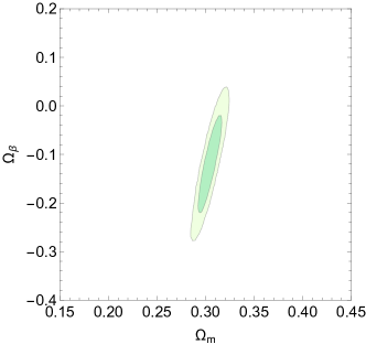
Figure 2: CASE III: 1$\sigma$ and 2$\sigma$ contours in the $\Omega_{m}$-$\Omega_{\beta}$ parameter space. Contours come from the joint of SNIa, $H(z)$, BAO and CMB data.

The Case V deserves special attention. Notice that from the combination of all data sets, the amount obtained of $\Omega_{\beta}$ suggests that it could account for cosmic acceleration. It is well known that the reduced $\chi^{2}$ gives us an idea of the quality of the fit, which should be close to 1 to be considered good. In this case the obtained $\chi^{2}_{r}=1.853$ is a little bit high. With this in mind we examined once again the scenario but taking out the CMB data. Then from the combined probes SNIa, OHD and BAO the obtained adjustment is $\Omega_{\beta}=-0.682^{+0.001}_{-0.003}$ with a $\chi^{2}_{r}=0.982$; from the normalization condition the best value for $\Omega_{dr}$ is $\Omega_{dr}=0.003^{+0.001}_{-0.003}$. These results are in excellent agreement with previous tests and additionally the fit is very good.

Finally, with the goal of getting more robust conclusions about the power of the MGBC model in explaining the current accelerated expansion, we perform an analysis by keeping free all the cosmological parameters, namely, $\Omega_{\beta}$, $\Omega_{dr}$, $\Omega_{m}$, $\Omega_{r}$ and $h$. With the normalization condition, the value for $\Omega_{\Lambda}$ can be obtained with $\Omega_{\Lambda}=1+\Omega_{\beta}-\Omega_{dr}-\Omega_{m}-\Omega_{r}$. By combining all the used data sets we get $\Omega_{\beta}=-0.024^{+0.112}_{-0.082}$, $\Omega_{dr}=0.007^{+0.012}_{-0.007}$, $\Omega_{m}=0.301^{+0.014}_{-0.019}$, $\Omega_{r}=[9.157^{+0.307}_{-0.652}]\times 10^{-5}$ and $h=0.690^{+0.035}_{-0.022}$ with $\chi^{2}_{r}=0.945$. One can immediately note that the fit is pretty good, but in cases with a non zero cosmological constant, $\Omega_{\beta}$ is not enough to produce the current cosmic acceleration, instead $\Omega_{\Lambda}$ contributes to the total of matter content with $\Omega_{\Lambda}=0.667^{+0.132}_{-0.082}$, in agreement with Planck results Ade et al. (2014).

On the other hand, in the cases with $\Omega_{\Lambda}=0$ (cases II, IV, V), from the combined analysis including the four probes (see table 7), it turned out that $\Omega_{\beta}$ is able to account for the accelerated expansion, and so the three of them, specially case V, are good candidates in favor of considering a geometrical origin of the accelerated expansion.

V Concluding Remarks

In this work it is examined how well the cosmological observations fit with the parameters of the modified geodetic brane cosmology (MGBC). Four probes have been considered: the supernovae Ia observations; the direct measurements of the Hubble parameter from differential evolution of passively evolving early-type galaxies; measurements of the distance ratio, $D_{V}/r_{s}$ gained from BAO measurements and finally, measurements of CMB shift parameters which provide an efficient summary of CMB data.

The set of parameters to be tested are $\theta_{i}=(\Omega_{m,0},\Omega_{\Lambda,0},\Omega_{\beta},\Omega_{dr})$, taken in pairs, fixing one of them and determining the fourth using the consistency relation; five cases were considered (see Table 1). For the first one were considered the following parameters I:$\theta_{i}=(\Omega_{\beta,0},\Omega_{dr},\Omega_{\Lambda,0})$ assuming the value of $\Omega_{m}=0.315\pm 0.012$ from the first Planck results Ade et al. (2014). It turns out that this case is unable to explain the cosmic acceleration without cosmological constant. The second case consist of the specifications II:$\theta_{i}=(\Omega_{\beta,0},\Omega_{dr},\Omega_{m,0})$ without cosmological constant $\Omega_{\Lambda,0}=0$; with this setting the right cosmological acceleration has its origin in the $\beta$ parameter; however the resulting matter content is a little bit smaller than the accepted value. The third case is proposed as III:$\theta_{i}=(\Omega_{\beta,0},\Omega_{m,0},\Omega_{\Lambda,0})$; $\Omega_{dr}$ is assumed to be the CMB radiation; the contribution of $\Omega_{\beta,0}$ is not enough to accelerate and cosmological constant is needed; the resulting matter content is correct; this case resembles pretty much the $\Lambda$CDM model. Case IV:$\theta_{i}=(\Omega_{\beta,0},\Omega_{m,0})$ without cosmological constant $\Omega_{\Lambda,0}=0$ and considering that $\Omega_{dr}$ is the CMB radiation; $\Omega_{\beta,0}$ accelerates the universe in the right amount but the matter content value is below to the accepted one.

The last and most promising case V is:$\theta_{i}=(\Omega_{\beta,0},\Omega_{dr})$ without cosmological constant $\Omega_{\Lambda,0}=0$ and assuming $\Omega_{m}=0.315\pm 0.012$; $\Omega_{\beta,0}$ accelerates the universe in the right amount. The best fit is obtained for this set of parameters with the joint probes SNIa, OHD and BAO, for redshifts in the range $0<z<1.75$. See Table 7 for a comparison of the adjustments of the five cases.

Finally it is remarkable that in cases with $\Omega_{\Lambda}=0$ (II, IV, V), the adjustment of $\Omega_{\beta}$ significantly increases its absolute value, supporting the argument that indeed $\Omega_{\beta}$ can play the role of a cosmological constant. The obtained results confirm that the currently observed accelerated expansion might have a geometrical origin, since the introduced parameter corresponding to the extrinsic curvature of the brane, is able to produce the observed acceleration.