Maxima of a randomized Riemann zeta function,
and branching random walks

Abstract.

A recent conjecture of Fyodorov–Hiary–Keating states that the maximum of the absolute value of the Riemann zeta function on a typical bounded interval of the critical line is $\exp\{\log\log T-\frac{3}{4}\log\log\log T+O(1)\}$, for an interval at (large) height $T$. In this paper, we verify the first two terms in the exponential for a model of the zeta function, which is essentially a randomized Euler product. The critical element of the proof is the identification of an approximate tree structure, present also in the actual zeta function, which allows us to relate the maximum to that of a branching random walk.

1. Introduction

The Riemann zeta function is defined for $\text{Re}(s)>1$ by a sum over integers, or equivalently by an Euler product over primes, as

(1) $$\zeta(s)=\sum_{n=1}^{\infty}\frac{1}{n^{s}}=\prod_{p\text{ primes}}(1-p^{-s})^{-1}\ ,$$

and by analytic continuation for other complex $s$. The behaviour of the function on the critical line $\text{Re}(s)=1/2$ is a major theme in number theory, the most important questions of course concerning the zeroes (e.g. the Riemann Hypothesis).

This paper is motivated by the study of the large values of $|\zeta(s)|$ on the critical line $s=1/2+it$. Little is known about the behavior on long intervals, say $0\leq t\leq T$ for $T$ large. The Lindelöf hypothesis, which is implied by the Riemann hypothesis, states that $\max_{0\leq t\leq T}|\zeta(1/2+it)|$ grows slower than any small power of $T$. See the paper of Farmer, Gonek and Hughes [12] for more precise conjectures about this maximum size, and the paper of Soundararajan [25] for a rigorous lower bound. More recently, Fyodorov, Hiary and Keating considered the maximum on bounded intervals of the critical line. They made the following conjecture:

Conjecture (Fyodorov–Hiary–Keating [14, 15]).

For $\tau$ sampled uniformly from $[0,T]$,

(2) $$\max_{h\in[0,1]}\log|\zeta(1/2+i(\tau+h))|=\log\log T-\frac{3}{4}\log\log\log T+O_{P}(1)\ ,$$

where $O_{P}(1)$ is a term that is stochastically bounded as $T\to\infty$.

The main result of this paper is a proof of the validity of the first two terms in (2) for a random model of $\zeta$ defined in (5) below, which is essentially a randomized Euler product. Until now such precise estimates were not known rigorously even for models of zeta.

The conjecture is intriguing for many reasons. From a number theory point of view, the precision of the prediction is striking. From a probability point of view, the leading and subleading order of the maximum correspond exactly to those of the maximum of a branching random walk (which is a collection of correlated random walks indexed by the leaves of a tree), as will be explained below. In fact, the key element of the proof for the random model will be the identification of an approximate tree structure for the zeta function.

1.1. Modelling the zeta function

If we take logarithms and Taylor expand the Euler product formula for the zeta function, we find for $\text{Re}(s)>1$,

(3) $$\log\zeta(s)=-\sum_{p}\log(1-p^{-s})=\sum_{k=1}^{\infty}\frac{1}{k}\sum_{p}\frac{1}{p^{ks}}=\sum_{p}\frac{1}{p^{s}}+O(1),\;\;\;\;\;$$

since the total contribution from all proper prime powers ($p^{ks}$ with $k\geq 2$) is uniformly bounded. One of the great challenges of analytic number theory is to understand how the influence of the Euler product may persist for general $s\in\mathbb{C}$. The definition of our random model is based on a rigorous result in that direction, assuming the truth of the Riemann Hypothesis, proved by Harper [19] by adapting a method of Soundararajan [26] (which itself builds heavily on classical work of Selberg [24]).

Proposition 1.1 (See Proposition 1 of Harper [19]).

Assume the Riemann Hypothesis. For $T$ large enough there exists a set $\mathcal{H}\subseteq[T,T+1]$, of measure at least $0.99$, such that

(4) $$\log|\zeta(1/2+it)|=\textup{Re}\left(\sum_{p\leq T}\frac{1}{p^{1/2+it}}\frac{\log(T/p)}{\log T}\right)+O(1)\;\;\;\;\;\forall t\in\mathcal{H}.$$

The set $\mathcal{H}$ produced in Proposition 1.1 consists of values $t$ that are not abnormally close, in a certain averaged sense, to many zeros of the zeta function. It seems reasonable to think that one shouldn’t typically find maxima very close to zeros. Moreover, if one only wants an upper bound then the restriction to the set $\mathcal{H}$ can in fact be removed, at the cost of a slightly more complicated right-hand side. Therefore, to understand the typical size of $\max_{0\leq h\leq 1}\log|\zeta(1/2+i(\tau+h))|$ as $\tau$ varies we should try to understand the typical size of $\max_{0\leq h\leq 1}\sum_{p\leq T}\text{Re}\left(\frac{1}{p^{1/2+i(\tau+h)}}\frac{\log(T/p)}{\log T}\right)$. The factor $\log(T/p)/\log T$ is a smoothing introduced for technical reasons. For simplicity we shall ignore it in our model.

Since the values of $\log p$ are linearly independent for distinct primes, it is easy to check by computing moments that the finite-dimensional distributions of the process $(p^{-i\tau},\text{ $p$ primes})$, where $\tau$ is sampled uniformly from $[0,T]$, converge as $T\rightarrow\infty$ to those of a sequence of independent random variables distributed uniformly on the unit circle. Following [19], this observation suggests to build a model from a probability space $(\Omega,\mathcal{F},\mathbb{P})$ with random variables $(U_{p},p\text{ primes})$ which are uniform on the unit circle, and independent. For $T>0$ and $h\in\mathbb{R}$, we consider the random variables $\sum_{p\leq T}p^{-1/2}\text{Re}(U_{p}p^{-ih})$. In view of Proposition 1.1, the process

(5) $$\left(\sum_{p\leq T}\frac{\text{Re}(U_{p}p^{-ih})}{p^{1/2}},h\in[0,1]\right)$$

seems like a reasonable model for the large values of $(\log|\zeta(1/2+i(\tau+h))|,h\in[0,1])$.

1.2. Main Result

In this paper, we provide evidence in favor of Conjecture Conjecture by proving a similar statement for the random model (5). At the same time, we hope to outline a possible approach to tackle the conjecture for the Riemann zeta function itself.

Theorem 1.2.

Let $(U_{p},p\text{ primes})$ be independent random variables on $(\Omega,\mathcal{F},\mathbb{P})$, distributed uniformly on the unit circle. Then

(6) $$\max_{h\in[0,1]}\sum_{p\leq T}\frac{\text{Re}(U_{p}p^{-ih})}{p^{1/2}}=\log\log T-\frac{3}{4}\log\log\log T+o_{P}(\log\log\log T),$$

where the sum is over the primes less than or equal to $T$ and the error term converges to $0$ in probability when divided by $\log\log\log T$.

An outline of the proof of the theorem is given in Section 1.4 below. The technical tools needed are developed in Section 2, and finally the proof is given in Section 3.

1.3. Relations to previous results

The leading order term $\log\log T$ in (6) was proved in [19], where it was also shown that the second order term must lie between $-2\log\log\log T$ and $-(1/4)\log\log\log T$. As well as giving a stronger result, our analysis here is ultimately based on a control of the joint distribution of only two points $h_{1}$ and $h_{2}$ of the random process at a time, which could feasibly be achieved for the zeta function itself. In contrast, the lower bound analysis in [19] depends on a Gaussian comparison inequality that requires control of $\log T$ points.

Fyodorov, Hiary and Keating motivated Conjecture Conjecture in [14, 15] using a connection to random matrices. There is convincing evidence, see e.g. [20], that the values of the zeta function in an interval of the critical line are well modelled by the characteristic polynomial $P_{N}(x)$ of an $N\times N$ matrix sampled uniformly from the unitary group, for $x=e^{i\theta}$ on the unit circle. In this spirit, they compute in [15] the moments of the partition function $Z_{N}(\beta)=\int_{0}^{2\pi}|P_{N}(e^{i\theta})|^{\beta}d\theta$. They argue that these coincide with those previously obtained for a logarithmically correlated Gaussian field [13]. For large $\beta$, this leads to the conjecture that the maximum of the characteristic polynomial behaves like the maximum of the Gaussian model. Unfortunately, the analogue of Conjecture Conjecture for this random matrix model is not known rigorously even to leading order (see [28] for recent developments at low $\beta$ and its relation to Gaussian multiplicative chaos). The conjecture is also expected to hold for other random matrix models such as the Gaussian Unitary Ensembles, see [16]. One advantage of the model (5) is that it can be analysed rigorously to a high level of precision with current probabilistic techniques.

As explained in Section 1.4, the proof of Theorem 1.2 uses in a crucial way an approximate tree structure present in our model and also in the actual zeta function. This structure explains the observed agreement between the high values of the zeta function and those of log-correlated random fields. The approach to control subleading orders of log-correlated Gaussian fields and branching random walks was first developed by Bramson [9] in his seminal work on the maximum of branching Brownian motion. It has since been extended to more general branching random walks by several authors, e.g. [1, 2, 11], and to log-correlated Gaussian fields, see for example [10, 22]. This type of argument can also be applied to obtain the joint distribution of the near-maxima, see e.g. [3, 4, 7]. Recently, a multiscale refinement of the second moment method was introduced by Kistler in [21] to control the leading and subleading orders of processes with neither a priori Gaussianity nor exact tree structure. It was successfully implemented in [5] to obtain the subleading order of cover times on the two-dimensional torus. The proof of Theorem 1.2 follows the same approach.

It is instructive to consider the conjecture in the light of the statistics of typical values of the zeta function. One beautiful result is the Selberg central limit theorem [24], which asserts that if $\tau$ is sampled uniformly from the interval $[0,T]$ then $(\frac{1}{2}\log\log T)^{-1/2}\log|\zeta(1/2+i\tau)|$ converges in law to a standard Gaussian variable. Thus, to obtain a rough prediction for the order of the maximum on $[0,1]$, one may compare it to the maximum of independent Gaussian variables of mean $0$ and variance $\frac{1}{2}\log\log T$. For $\log T$ such variables, it is not hard to show that the order of the maximum is $\log\log T-\frac{1}{4}\log\log\log T+O(1)$. The leading order agrees with Conjecture Conjecture, but the constant in the subleading correction is different. Our proof shows how to modify this “independent” heuristic to account for the “extra” $-\frac{1}{2}\log\log\log T$ present in Conjecture Conjecture. Bourgade showed a multivariate version of Selberg’s theorem where the correlations are logarithmic in the limit [8]. However, the convergence is too weak to describe the maximum on an interval.

1.4. Outline of the proof

The proof of Theorem 1.2 is based on an analogy between the process (5) and a branching random walk (also known as hierarchical random field). We make this connection precise here, and indicate for an unfamiliar reader how to analyse the maximum of a branching random walk.

We will work in the case where $T=e^{2^{n}}$ for some large natural number $n$. In this setup, the process of interest in Theorem 1.2 is

(7) $$(X_{n}(h),h\in[0,1])\ ,\qquad\text{ where }\ X_{n}(h)=\sum_{p\leq e^{2^{n}}}\frac{\text{Re}(U_{p}p^{-ih})}{p^{1/2}}\$$

is a continuous function of $h$. Since $\log\log T=n\log 2$ and $\log\log\log T=\log n+O(1)$, Theorem 1.2 can be restated as:

(8) $$\displaystyle{\lim_{n\to\infty}}\mathbb{P}\left[m_{n}(-\varepsilon)\leq\max_{h\in[0,1]}X_{n}(h)\leq m_{n}(\varepsilon)\right]=1\mbox{, for all }\varepsilon>0,$$

(9) $$\text{where }m_{n}(\varepsilon)=n\log 2-\frac{3}{4}\log n+\varepsilon\log n\ .$$

In other words, with large probability, the maximum of the process lies in an arbitrarily small window (of order $\log n$) around $n\log 2-\frac{3}{4}\log n$.

By symmetry of $U_{p}$ we have $\mathbb{E}[X_{n}(h)]=0$ for any $h\in[0,1]$. Also a simple computation shows that $\mathbb{E}[\text{Re}(U_{p}p^{-ih})\text{Re}(U_{p}p^{-ih^{\prime}})]=(1/2)\cos(|h-h^{\prime}|\log p)$, so the covariance $\mathbb{E}[X_{n}(h)X_{n}(h^{\prime})]$ equals $\frac{1}{2}\sum_{\log p\leq 2^{n}}p^{-1}\cos(|h-h^{\prime}|\log p)$. Using well known results on primes (cf. Lemma 2.1), it is possible to estimate this as

(10) $$\mathbb{E}\left[X_{n}(h)X_{n}(h^{\prime})\right]\approx\frac{1}{2}\log|h-h^{\prime}|^{-1},$$

for any $h,h^{\prime}\in[0,1]$ provided $|h-h^{\prime}|\geq 2^{-n}$. If instead $|h-h^{\prime}|<2^{-n}$, then the covariance is almost $n(\log 2)/2$, i.e. $X_{n}(h)$ and $X_{n}(h^{\prime})$ are almost perfectly correlated. Therefore, one can think of the maximum over $h\in[0,1]$ as a maximum over $2^{n}$ equally spaced points.

The key point of the proof is that the logarithmic nature of the correlations can be understood in a more structural way using a multiscale decomposition. Precisely, we rewrite the process as

(11) $$X_{n}(h)=\sum_{k=0}^{n}Y_{k}(h),\;\;\;\text{where}\;Y_{k}(h)=\sum_{2^{k-1}<\log p\leq 2^{k}}\frac{\text{Re}(U_{p}p^{-ih})}{p^{1/2}}\ ,$$

is the increment at “scale” $k$ of $X_{n}(h)$. It is not hard to show, see Section 2.1, that for $k$ large,

(12) $$\mathbb{E}\left[Y_{k}(h)^{2}\right] \approx\frac{\log 2}{2},\quad\mbox{ and}\quad\mathbb{E}\left[Y_{k}(h)Y_{k}(h^{\prime})\right] \approx\begin{cases}\frac{\log 2}{2}&\text{ if $|h-h^{\prime}|\leq 2^{-k}$},\\ 0&\text{ if $|h-h^{\prime}|>2^{-k}$.}\end{cases}$$

In view of (12), for given $h,h^{\prime}$, one can think of the partial sums $X_{k}(h)=\sum_{j=1}^{k}Y_{j}(h)$ and $X_{k}(h^{\prime})=\sum_{j=1}^{k}Y_{j}(h^{\prime})$ as random walks, where the increments $Y_{j}(h),Y_{j}(h^{\prime})$ are almost perfectly correlated (so roughly the same) for those $j$ such that $2^{j}\leq|h-h^{\prime}|^{-1}$, and where they are almost perfectly decorrelated (so essentially independent) when $2^{j}>|h-h^{\prime}|^{-1}$. A similar, but exact, behaviour would be obtained as follows: Consider $2^{n}$ equally spaced points in $[0,1]$, thought of as leaves of a binary tree of depth $n$. Place on each edge of the binary tree an independent Gaussian with mean zero and variance $(\log 2)/2$, and associate to a leaf the random walk given by the partial sums of the Gaussians on the path from root to leaf, see Figure 1. With this construction, the first $k$ increments of the random walks of two leaves will be exactly the same, where $k$ is the level of the most recent common ancestor, and the rest of the increments will be perfectly independent. This tree construction is an example of branching random walk. For the model (7) of zeta, the branching point $k$ where the paths $X_{k}(h)$ and $X_{k}(h^{\prime})$ roughly decorrelate is

(13) $$h\wedge h^{\prime}=\lfloor\log_{2}|h-h^{\prime}|^{-1}\rfloor\ .$$

So $h$ and $h^{\prime}$ correspond to leaves whose most recent common ancestor is in level $k=h\wedge h^{\prime}$. We note that the different nature of the correlations for different ranges of $p$ was already exploited in early work of Halász [18], although without drawing any connection to branching.

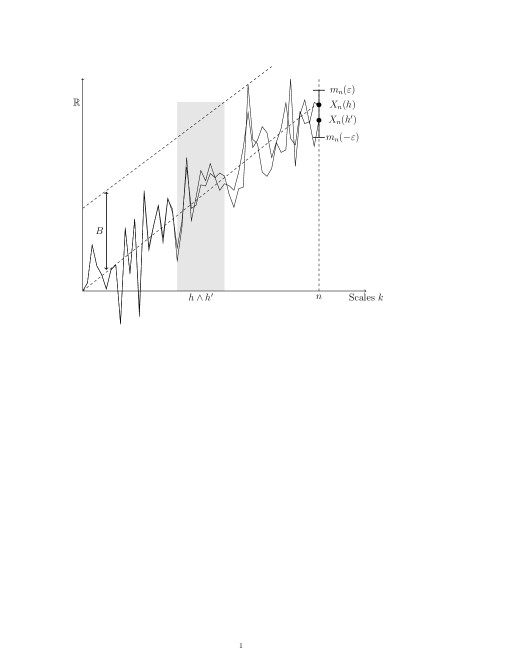
Figure 1. (Left) An illustration of the correlation structure of a branching random walk. (Right) A realization of two paths of an approximate branching random walk with increments almost equal before the branching point $h\wedge h^{\prime}$ and almost decoupled after. The barrier below which the paths must stay is also shown.

A compelling method to analyse the maximum of a branching random walk and of log-correlated processes in general is a multiscale refinement of the second moment method as proposed in [21], which we implement to the approximate branching setting described above. Naively, one could first consider the number of variables whose value exceeds a given value $m$, i.e. the number of exceedances,

(14) $$Z(m)=\#\{j\leq 2^{n}:X_{n}(j/2^{n})\geq m\}\ .$$

Clearly, $\max_{j\leq 2^{n}}X_{n}(j/2^{n})\geq m$ if and only if $Z(m)\geq 1$. Thus an upper bound for the maximum can be obtained by the union bound

(15) $$\mathbb{P}(Z(m)\geq 1)\leq\mathbb{E}[Z(m)]=2^{n}\mathbb{P}(X_{n}(0)\geq m)\ .$$

On the other hand, a lower bound can be obtained by the Paley–Zygmund inequality,

(16) $$\mathbb{P}(Z(m)\geq 1)\geq\frac{\mathbb{E}[Z(m)]^{2}}{\mathbb{E}[Z(m)^{2}]}\ .$$

More precisely, one would choose $m=m(n)$ large enough in (15) so that $\mathbb{E}[Z(m)]=o(1)$, and $m$ small enough in (16) so that $\mathbb{E}[Z]^{2}=(1+o(1))\mathbb{E}[Z^{2}]$, and thus $\mathbb{P}(Z(m)\geq 1)=1+o(1)$. For this one needs large deviation estimates: if we think of $X_{n}(h)$ as Gaussian with variance $n\log 2/2$, then a standard Gaussian estimate yields that $P(X_{n}(h)\geq m)$ is approximately $\frac{\sqrt{n}}{m}e^{-m^{2}/((\log 2)n)}$. Thus $2^{n}P(X_{n}(0)\geq m)=o(1)$ when $m=(\log 2)n-\frac{1}{4}\log n+\varepsilon\log n$. This would in fact be the correct answer (the union bound would be sharp) if the random variables $X_{n}(j/2^{n})$ were independent. However, if $m=(\log 2)n-\frac{3}{4}\log n+\varepsilon\log n$, then $2^{m}\mathbb{P}(X_{n}(0)\geq m)\geq cn^{1-\varepsilon}\to\infty$, so (15) cannot prove the upper bound we seek in Theorem 1.2. Similarly, the right-hand side of (16) will tend to zero unless $m\leq\frac{\log 2}{2}n$, since strong correlation between exceedance events for nearby $h,h^{\prime}$ inflates the second moment. Thus the lower bound obtained is not close to what we seek even to leading order.

To get tight bounds, one needs to modify the definition of the number of exceedances using an insight from the underlying approximate tree structure. For branching random walk there are exactly $2^{k}$ distinct partial sums up to the $k$-level, one for each vertex at that level. By analogy one expects that the “variation” in $X_{k}(h)$ (i.e. in the partial sums up to the $k$-th level) for different $h\in[0,1]$ should be captured by just $2^{k}$ equally spaced points in $[0,1]$. Even if they were independent, it would be very unlikely that one of these $2^{k}$ values exceeded $k\log 2+B$, for $B>0$ growing slowly with $n$, and it turns out that positive correlations only make it less likely. This can be proved using elementary arguments, cf. Lemma 3.4. In other words, with high probability, all random walks $X_{k}(h)$ must lie below the barrier $k\mapsto k\log 2+B$. This suggests to look at the modified number of exceedances

(17) $$\widetilde{Z}(m)=\#\{j\leq 2^{n}:X_{n}(j/2^{n})\geq m,X_{k}(j/2^{n})<k\log 2+B\ ,\forall k\leq n\}\ .$$

It turns out that replacing $Z$ by $\widetilde{Z}$ in the first moment bound (15) and (with slight modifications) in the second moment bound (16) will yield the correct answer. To see this in the former case, we write the first moment by conditioning on the end point:

(18) $$\mathbb{E}[\widetilde{Z}(m)]=2^{n}\mathbb{P}(X_{n}(0)>m)\times\mathbb{P}(X_{k}(0)<k\log 2+B\ ,\forall k\leq n|X_{n}(0)>m)\ .$$

By the earlier naive discussion, the first two terms amount to $O(n^{1-\varepsilon})$ when we set $m=n\log 2-\frac{3}{4}\log n+\varepsilon\log n$. The third term is the probability that a random walk bridge starting at $0$ and ending at $m=n\log 2-\frac{3}{4}\log n+\varepsilon\log n$ avoids the barrier $k\log 2+B$. This probability turns out to be $n^{-1}$, as shown by the ballot theorem, cf. Lemma 2.12. Therefore, $\mathbb{E}[\widetilde{Z}(m)]=O(n^{-\varepsilon})\to 0$, for all $\varepsilon>0$. A similar analysis can be done for the lower bound, where we have the obvious inequality $\mathbb{P}(Z(m)\geq 1)\geq\mathbb{P}(\widetilde{Z}(m)\geq 1)$. The extra barrier condition turns out to reduce correlations between exceedance events sufficiently so that the second moment is now essentially the first moment squared when $m\leq n\log 2-\frac{3}{4}\log n-\varepsilon\log n$ (this indicates why the second moment of $Z(m)$ is too large: in the exponentially unlikely event that a path manages to go far above the barrier, it has exponentially many “offspring” that end up far above the typical level of the maximum).

The form of the subleading correction is thus explained by the extra “cost” $n^{-1}$ of satisfying the barrier condition. And the barrier condition arises because of “tree-like” correlations present in the values of (the model of) the zeta function. This suggests the possibility that the partial sums of the Euler product (3) of the actual zeta function behave similarly where the zeta function is large.

To prove Theorem 1.2, we must address the imprecisions in the above discussion. The necessary large deviation estimates are derived in Section 2.1. The claim that $X_{k}(h)$ does not vary much below scale $2^{-k}$ is proved in Section 2.2 using a chaining argument. Another issue is that our process is not an exact branching random walk because increments are never perfectly independent (for different $h,h^{\prime}$) nor exactly identical. To deal with this, we use a Berry–Esseen approximation in Section 2.3 to show that the random walks are very close to being Gaussian. This allows for an explicit comparison with Gaussian random walks with i.i.d. increments and “perfect” branching. Moreover, to get a sharp lower bound with the second moment method, it is necessary to “cut off the first $r$ scales” and consider

(19) $$X_{r,k}(h)=X_{k}(h)-X_{r}(h)\qquad\text{for $h\in\mathbb{R}$, }$$

for an appropriately chosen $r$. Finally, it should be stressed that our approach relies only on controlling first and second moments, which means that the estimates we need only involve at most two random walks simultaneously.

2. Preliminaries

Throughout the paper, we will write $c$ for absolute constants whose value may change at different occurrences. A sum over the variable $p$ always denotes a sum over primes.

2.1. Large Deviation Estimates

In this section, we derive the large deviation properties of the increments $(Y_{k}(h),h\in[0,1])$ and their sum. We first derive basic facts on their distribution and in particular on their correlations.

Recall that the random variables $(U_{p},p\text{ primes})$ are i.i.d. and uniform on the unit circle. For simplicity, we denote the $p$-th term of the sum over primes in (6) by,

(20) $$W_{p}(h)=\frac{\text{Re}(U_{p}p^{-ih})}{p^{1/2}},h\in\mathbb{R}.$$

Note that the law of the process $(W_{p}(h),h\in\mathbb{R})$ is translation-invariant on the real line and also invariant under the reflection $h\mapsto-h$. A straightforward computation using the law of the $U_{p}$’s and translation invariance gives

(21) $$\mathbb{E}\left[W_{p}(h)W_{p}(h^{\prime})\right]=\frac{1}{2p}\cos(|h-h^{\prime}|\log p),\text{ for all $h,h^{\prime}$. }$$

In this notation, the increments defined in (11) are

(22) $$Y_{k}(h)=\sum_{2^{k-1}<\log p\leq 2^{k}}W_{p}(h),h\in\mathbb{R}.$$

Using (21) and the independence of the $U_{p}$’s, the variance of $Y_{k}(h)$ becomes

(23) $$\sigma_{k}^{2}=\text{Var}(Y_{k}(h))=\sum_{2^{k-1}<\log p\leq 2^{k}}\frac{1}{2p}\ ,$$

and the covariance of $Y_{k}(h)$ and $Y_{k}(h^{\prime})$ is,

(24) $$\rho_{k}(h,h^{\prime})=\mathbb{E}[Y_{k}(h)Y_{k}(h^{\prime})]=\sum_{2^{k-1}<\log p\leq 2^{k}}\frac{1}{2p}\cos(|h-h^{\prime}|\log p).$$

The next lemma formalizes (12), giving bounds for how close the variance of the increments is to

(25) $$\sigma^{2}=(\log 2)/2\ ,$$

and for $h\neq h^{\prime}$, how close the covariance is to the variance before the ”branching point” $h\wedge h^{\prime}$, defined in (13), and how fast it decays after.

Lemma 2.1.

For $h,h^{\prime}\in\mathbb{R}$ and $k\geq 1$,

(26) $$\sigma_{k}^{2}=\mathbb{E}\left[Y_{k}(h)^{2}\right]=\sigma^{2}+O\left(e^{-c\sqrt{2^{k}}}\right),$$

(27) $$\rho_{k}(h,h^{\prime})=\mathbb{E}\left[Y_{k}(h)Y_{k}(h^{\prime})\right]=\begin{cases}\sigma^{2}+O\left(2^{-2(h\wedge h^{\prime}-k)}\right)+O\left(e^{-c\sqrt{2^{k}}}\right)&\text{ if $k\leq h\wedge h^{\prime}$,}\\ O\left(2^{-(k-h\wedge h^{\prime})}\right)&\text{ if $k>h\wedge h^{\prime}$.}\end{cases}$$

Note that in both cases the error term decays exponentially in $k$.

Proof.

We use a strong form of the Prime Number Theorem (see Theorem 6.9 of [23]) which states that

(28) $$\#\{p\leq x:p\mbox{ prime}\}=\int_{2}^{x}\frac{1}{\log u}du+O(xe^{-c\sqrt{\log x}}).$$

By replacing the sum $\sum_{P<p\leq Q}\frac{1}{p}$ with the integral $\int_{P}^{Q}\frac{1}{u\log u}du$ using (28) and integration by parts, one obtains

$$\sum_{P<p\leq Q}\frac{1}{p}=\log\log Q-\log\log P+O(e^{-c\sqrt{\log P}}),\mbox{ for all }2\leq P\leq Q.$$

This together with (23) yields (26). Similarly (28) implies that

$$\rho_{k}(h,h^{\prime})=\frac{1}{2}\int_{e^{2^{k-1}}}^{e^{2^{k}}}\frac{\cos(|h-h^{\prime}|\log u)}{u\log u}du+O\left((1+|h-h^{\prime}|)e^{-c\sqrt{2^{k-1}}}\right).$$

When $2^{k}|h-h^{\prime}|=2^{k-h\wedge h^{\prime}}\leq 1$, the claim (27) follows by using that $\cos(|h-h^{\prime}|\log u)=1+O(|h-h^{\prime}|^{2}(\log u)^{2})$. When $2^{-k}|h-h^{\prime}|^{-1}=2^{-k+h\wedge h^{\prime}}<1$, we use integration by parts. After the change of variable $v=\log u$, the integral becomes

$$\frac{\sin(|h-h^{\prime}|v)}{|h-h^{\prime}|v}\Big{|}_{2^{k-1}}^{2^{k}}+\int_{2^{k-1}}^{2^{k}}\frac{\sin(|h-h^{\prime}|v)}{|h-h^{\prime}|v^{2}}du\ .$$

Both terms are $O(2^{-k}|h-h^{\prime}|^{-1})$.

∎

Remark 1.

A similar but easier argument using (28) shows that

(29) $$\sum_{P<p\leq Q}\frac{\left(\log p\right)^{m}}{p}=O((\log Q)^{m}),\mbox{ for all }1\leq P\leq Q.$$

The main results of this section are explicit expressions for the cumulant generating functions of the increments, from which we will deduce large deviation estimates. For fixed $h,h^{\prime}\in\mathbb{R}$, we will often drop the dependence on $h$ and $h^{\prime}$ when it is clear from context and define

$$\mathchoice{\mbox{\boldmath$\displaystyle Y$}}{\mbox{\boldmath$\textstyle Y$}}{\mbox{\boldmath$\scriptstyle Y$}}{\mbox{\boldmath$\scriptscriptstyle Y$}}_{k}=\big{(}Y_{k}(h),Y_{k}(h^{\prime})\big{)}\ .$$

The covariance matrix of $\mathchoice{\mbox{\boldmath$\displaystyle Y$}}{\mbox{\boldmath$\textstyle Y$}}{\mbox{\boldmath$\scriptstyle Y$}}{\mbox{\boldmath$\scriptscriptstyle Y$}}_{k}$ is then denoted by

$$\mathchoice{\mbox{\boldmath$\displaystyle\Sigma$}}{\mbox{\boldmath$\textstyle\Sigma$}}{\mbox{\boldmath$\scriptstyle\Sigma$}}{\mbox{\boldmath$\scriptscriptstyle\Sigma$}}_{k}=\text{Cov}(\mathchoice{\mbox{\boldmath$\displaystyle Y$}}{\mbox{\boldmath$\textstyle Y$}}{\mbox{\boldmath$\scriptstyle Y$}}{\mbox{\boldmath$\scriptscriptstyle Y$}}_{k})=\left(\begin{array}[]{cc}\sigma_{k}^{2}&\rho_{k}\\ \rho_{k}&\sigma_{k}^{2}\end{array}\right)\ .$$

The eigenvalues of $\Sigma_{k}$ are $\sigma_{k}^{2}\pm\rho_{k}$.

The cumulant generating functions are

(30) $$\psi^{(1)}_{k}(\lambda)=\log\mathbb{E}[\exp(\lambda Y_{k})]\qquad\psi^{(2)}_{k}(\mathchoice{\mbox{\boldmath$\displaystyle\lambda$}}{\mbox{\boldmath$\textstyle\lambda$}}{\mbox{\boldmath$\scriptstyle\lambda$}}{\mbox{\boldmath$\scriptscriptstyle\lambda$}})=\log\mathbb{E}[\exp(\mathchoice{\mbox{\boldmath$\displaystyle\lambda$}}{\mbox{\boldmath$\textstyle\lambda$}}{\mbox{\boldmath$\scriptstyle\lambda$}}{\mbox{\boldmath$\scriptscriptstyle\lambda$}}\cdot\mathchoice{\mbox{\boldmath$\displaystyle Y$}}{\mbox{\boldmath$\textstyle Y$}}{\mbox{\boldmath$\scriptstyle Y$}}{\mbox{\boldmath$\scriptscriptstyle Y$}}_{k})]\ ,$$

where $\lambda\in\mathbb{R}$, $\mathchoice{\mbox{\boldmath$\displaystyle\lambda$}}{\mbox{\boldmath$\textstyle\lambda$}}{\mbox{\boldmath$\scriptstyle\lambda$}}{\mbox{\boldmath$\scriptscriptstyle\lambda$}}\in\mathbb{R}^{2}$ and $``\cdot"$ is the inner product in $\mathbb{R}^{2}$. The following change of measure will also be needed in the proof of Theorem 1.2:

(31) $$\frac{d\mathbb{Q}_{\lambda}}{d\mathbb{P}}=\prod_{k=1}^{n}\frac{e^{\lambda Y_{k}}}{e^{\psi^{(1)}_{k}(\lambda)}}\ \mbox{ for }\lambda\in\mathbb{R},\quad\quad\quad\frac{d\mathbb{Q}_{\mathchoice{\mbox{\boldmath$\displaystyle\lambda$}}{\mbox{\boldmath$\textstyle\lambda$}}{\mbox{\boldmath$\scriptstyle\lambda$}}{\mbox{\boldmath$\scriptscriptstyle\lambda$}}}}{d\mathbb{P}}=\prod_{k=1}^{n}\frac{e^{\mathchoice{\mbox{\boldmath$\displaystyle\lambda$}}{\mbox{\boldmath$\textstyle\lambda$}}{\mbox{\boldmath$\scriptstyle\lambda$}}{\mbox{\boldmath$\scriptscriptstyle\lambda$}}\cdot\mathchoice{\mbox{\boldmath$\displaystyle Y$}}{\mbox{\boldmath$\textstyle Y$}}{\mbox{\boldmath$\scriptstyle Y$}}{\mbox{\boldmath$\scriptscriptstyle Y$}}_{k}}}{e^{\psi^{(2)}_{k}(\mathchoice{\mbox{\boldmath$\displaystyle\lambda$}}{\mbox{\boldmath$\textstyle\lambda$}}{\mbox{\boldmath$\scriptstyle\lambda$}}{\mbox{\boldmath$\scriptscriptstyle\lambda$}})}}\ \mbox{ for }\mathchoice{\mbox{\boldmath$\displaystyle\lambda$}}{\mbox{\boldmath$\textstyle\lambda$}}{\mbox{\boldmath$\scriptstyle\lambda$}}{\mbox{\boldmath$\scriptscriptstyle\lambda$}}\in\mathbb{R}^{2}.$$

Recall that in the univariate case,

(32) $$\mathbb{Q}_{\lambda}[Y_{k}]=\frac{d}{d\lambda}\psi_{k}^{(1)}(\lambda),\qquad\text{Var}_{\mathbb{Q}_{\lambda}}(Y_{k})=\frac{d^{2}}{d\lambda^{2}}\psi_{k}^{(1)}(\lambda)\ ,$$

and in the multivariate case,

(33) $$\mathbb{Q}_{\mathchoice{\mbox{\boldmath$\displaystyle\lambda$}}{\mbox{\boldmath$\textstyle\lambda$}}{\mbox{\boldmath$\scriptstyle\lambda$}}{\mbox{\boldmath$\scriptscriptstyle\lambda$}}}[\mathchoice{\mbox{\boldmath$\displaystyle Y$}}{\mbox{\boldmath$\textstyle Y$}}{\mbox{\boldmath$\scriptstyle Y$}}{\mbox{\boldmath$\scriptscriptstyle Y$}}_{k}]=\nabla\psi_{k}^{(2)}(\mathchoice{\mbox{\boldmath$\displaystyle\lambda$}}{\mbox{\boldmath$\textstyle\lambda$}}{\mbox{\boldmath$\scriptstyle\lambda$}}{\mbox{\boldmath$\scriptscriptstyle\lambda$}}),\qquad\text{Cov}_{\mathbb{Q}_{\mathchoice{\mbox{\boldmath$\displaystyle\lambda$}}{\mbox{\boldmath$\textstyle\lambda$}}{\mbox{\boldmath$\scriptstyle\lambda$}}{\mbox{\boldmath$\scriptscriptstyle\lambda$}}}}(\mathchoice{\mbox{\boldmath$\displaystyle Y$}}{\mbox{\boldmath$\textstyle Y$}}{\mbox{\boldmath$\scriptstyle Y$}}{\mbox{\boldmath$\scriptscriptstyle Y$}}_{k})=\text{Hess}\ \psi_{k}^{(2)}(\mathchoice{\mbox{\boldmath$\displaystyle\lambda$}}{\mbox{\boldmath$\textstyle\lambda$}}{\mbox{\boldmath$\scriptstyle\lambda$}}{\mbox{\boldmath$\scriptscriptstyle\lambda$}})\ .$$

The results also provide bounds on these quantities. We first state the result for the univariate case. The proof is omitted since it is a special case of the multivariate bound in Proposition 2.4.

Proposition 2.2.

Let $C>0$. For all $0<\lambda<C$ and $k$ large enough (depending on $C$), the cumulant generating function $\psi_{k}^{\left(1\right)}\left(\lambda\right)$ satisfies

(34) $$\psi_{k}^{\left(1\right)}\left(\lambda\right)=\frac{\lambda^{2}\sigma_{k}^{2}}{2}+O\left(e^{-2^{k-1}}\right)\ .$$

Moreover, for such $k$, the measure $\mathbb{Q}_{\lambda}$ in (31) satisfies

(35) $$\mathbb{Q}_{\lambda}\left[Y_{k}\right]=\lambda\sigma_{k}^{2}+O\left(e^{-2^{k-1}}\right),\qquad Var_{\mathbb{Q}_{\lambda}}\left[Y_{k}\right]=\sigma_{k}^{2}+O\left(e^{-2^{k-1}}\right)\ .$$

One useful consequence of the proposition is a one-point large deviation estimate, which after being strengthened to a bound for the maximum over a small interval, will be a crucial input to the proof of the upper bound of Theorem 1.2 (see (44) and (74)). Recall from (19) that $X_{r,k}(h)=X_{k}(h)-X_{r}(h)=\sum_{l=r+1}^{k}Y_{l}(h)$.

Corollary 2.3.

Let $C>0$. For any $0\leq r\leq k-1$, $0<x<C(k-r)$ and $h\in\mathbb{R}$,

(36) $$\mathbb{P}\left[X_{r,k}\left(h\right)>x\right]\leq c\exp\left(-\frac{x^{2}}{2(k-r)\sigma^{2}}\right),$$

where the constant $c$ depends on $C$.

Proof.

Using the exponential Chebyshev’s inequality, the probability in (36) is bounded above by $\exp\left(\sum_{l=r+1}^{k}\psi_{l}^{\left(1\right)}\left(\lambda\right)-\lambda x\right)$, for all $\lambda>0$. By Proposition 2.2 (with, say, $10C$ in place of $C$), we get that if $\lambda\leq 10C$,

$$\mathbb{P}\left[X_{r,k}\left(h\right)>x\right] \leq\exp\left(c+\frac{\lambda^{2}}{2}\sum_{l=r+1}^{k}\sigma_{l}^{2}-\lambda x+O(e^{-c2^{r}})\right)$$

$$\leq c\exp\left(\frac{\lambda^{2}}{2}\sum_{l=r+1}^{k}\sigma_{l}^{2}-\lambda x\right)\overset{\eqref{eqn: sigmak estimate}}{\leq}c\exp\left(\frac{\lambda^{2}}{2}\left(k-r\right)\sigma^{2}-\lambda x\right),$$

where for $l$ too small for (34) to be applied, we simply use that $\psi_{l}(\lambda)$ is bounded. Setting $\lambda=x\big{(}(k-r)\sigma^{2}\big{)}^{-1}\leq 10C$ gives the result. ∎

We now prove the bounds in the multivariate case.

Proposition 2.4.

Let $C>0$. For all $\mathchoice{\mbox{\boldmath$\displaystyle\lambda$}}{\mbox{\boldmath$\textstyle\lambda$}}{\mbox{\boldmath$\scriptstyle\lambda$}}{\mbox{\boldmath$\scriptscriptstyle\lambda$}}=\left(\lambda,\lambda^{{}^{\prime}}\right)$, where $0<\lambda,\lambda^{\prime}<C$, and $k$ large enough (depending on $C$), the cumulant generating function $\psi_{k}^{\left(2\right)}\left(\mathchoice{\mbox{\boldmath$\displaystyle\lambda$}}{\mbox{\boldmath$\textstyle\lambda$}}{\mbox{\boldmath$\scriptstyle\lambda$}}{\mbox{\boldmath$\scriptscriptstyle\lambda$}}\right)$ satisfies

(37) $$\psi_{k}^{(2)}\big{(}\mathchoice{\mbox{\boldmath$\displaystyle\lambda$}}{\mbox{\boldmath$\textstyle\lambda$}}{\mbox{\boldmath$\scriptstyle\lambda$}}{\mbox{\boldmath$\scriptscriptstyle\lambda$}}\big{)}=\frac{1}{2}\mathchoice{\mbox{\boldmath$\displaystyle\lambda$}}{\mbox{\boldmath$\textstyle\lambda$}}{\mbox{\boldmath$\scriptstyle\lambda$}}{\mbox{\boldmath$\scriptscriptstyle\lambda$}}\cdot\mathchoice{\mbox{\boldmath$\displaystyle\Sigma$}}{\mbox{\boldmath$\textstyle\Sigma$}}{\mbox{\boldmath$\scriptstyle\Sigma$}}{\mbox{\boldmath$\scriptscriptstyle\Sigma$}}_{k}\mathchoice{\mbox{\boldmath$\displaystyle\lambda$}}{\mbox{\boldmath$\textstyle\lambda$}}{\mbox{\boldmath$\scriptstyle\lambda$}}{\mbox{\boldmath$\scriptscriptstyle\lambda$}}+O\big{(}e^{-2^{k-1}}\big{)}.$$

Moreover, for such $k$, the measure $\mathbb{Q}_{\mathchoice{\mbox{\boldmath$\displaystyle\lambda$}}{\mbox{\boldmath$\textstyle\lambda$}}{\mbox{\boldmath$\scriptstyle\lambda$}}{\mbox{\boldmath$\scriptscriptstyle\lambda$}}}$ in (31) satisfies

(38) $$\mathbb{Q}_{\mathchoice{\mbox{\boldmath$\displaystyle\lambda$}}{\mbox{\boldmath$\textstyle\lambda$}}{\mbox{\boldmath$\scriptstyle\lambda$}}{\mbox{\boldmath$\scriptscriptstyle\lambda$}}}\left[\mathchoice{\mbox{\boldmath$\displaystyle Y$}}{\mbox{\boldmath$\textstyle Y$}}{\mbox{\boldmath$\scriptstyle Y$}}{\mbox{\boldmath$\scriptscriptstyle Y$}}_{k}\right]=\mathchoice{\mbox{\boldmath$\displaystyle\Sigma$}}{\mbox{\boldmath$\textstyle\Sigma$}}{\mbox{\boldmath$\scriptstyle\Sigma$}}{\mbox{\boldmath$\scriptscriptstyle\Sigma$}}_{k}\mathchoice{\mbox{\boldmath$\displaystyle\lambda$}}{\mbox{\boldmath$\textstyle\lambda$}}{\mbox{\boldmath$\scriptstyle\lambda$}}{\mbox{\boldmath$\scriptscriptstyle\lambda$}}+O\big{(}e^{-2^{k-1}}\big{)}\mbox{ and }\text{Cov}_{\mathbb{Q}_{\lambda}}\left[\mathchoice{\mbox{\boldmath$\displaystyle Y$}}{\mbox{\boldmath$\textstyle Y$}}{\mbox{\boldmath$\scriptstyle Y$}}{\mbox{\boldmath$\scriptscriptstyle Y$}}{}_{k}\right]=\mathchoice{\mbox{\boldmath$\displaystyle\Sigma$}}{\mbox{\boldmath$\textstyle\Sigma$}}{\mbox{\boldmath$\scriptstyle\Sigma$}}{\mbox{\boldmath$\scriptscriptstyle\Sigma$}}_{k}+O\big{(}e^{-2^{k-1}}\big{)}.$$

Proof.

We first compute

(39) $$\begin{array}[]{rcl}\psi_{p}^{W}(\mathchoice{\mbox{\boldmath$\displaystyle\lambda$}}{\mbox{\boldmath$\textstyle\lambda$}}{\mbox{\boldmath$\scriptstyle\lambda$}}{\mbox{\boldmath$\scriptscriptstyle\lambda$}})&=&\log\mathbb{E}[\exp(\lambda W_{p}(0)+\lambda^{\prime}W_{p}(|h-h^{\prime}|)]\\ &=&\log\frac{1}{2\pi}\int_{0}^{2\pi}\exp\left(\frac{\lambda}{p^{1/2}}\cos(\theta)+\frac{\lambda^{\prime}}{p^{1/2}}\cos(\theta+|h-h^{\prime}|\log p)\right)d\theta.\end{array}$$

Recall that for any $a,b\in\mathbb{R}$,

(40) $$\frac{1}{2\pi}\int_{0}^{2\pi}\exp(a\cos(\theta)+b\sin(\theta))d\theta=I_{0}(\sqrt{a^{2}+b^{2}}),$$

where $I_{n}$ denotes the $n$-th modified Bessel function of the first kind. The identity $\cos(\theta+\eta)=\cos(\theta)\cos(\eta)-\sin(\theta)\sin(\eta)$ can be used together with (40) to write the integral in the bottom line of (39) as

(41) $$\begin{array}[]{l}I_{0}\left(\sqrt{\frac{1}{p}\left(\lambda+\cos(|h-h^{\prime}|\log p)\lambda^{\prime}\right)^{2}+\frac{1}{p}\left(\sin(|h-h^{\prime}|\log p)\lambda^{\prime}\right)^{2}}\right)\\ =I_{0}\left(\sqrt{\frac{1}{p}\left(\lambda^{2}+2\lambda\lambda^{\prime}\cos(|h-h^{\prime}|\log p)+\lambda^{\prime 2}\right)}\right)=I_{0}\left(\sqrt{2\mathchoice{\mbox{\boldmath$\displaystyle\lambda$}}{\mbox{\boldmath$\textstyle\lambda$}}{\mbox{\boldmath$\scriptstyle\lambda$}}{\mbox{\boldmath$\scriptscriptstyle\lambda$}}\cdot\mathchoice{\mbox{\boldmath$\displaystyle M$}}{\mbox{\boldmath$\textstyle M$}}{\mbox{\boldmath$\scriptstyle M$}}{\mbox{\boldmath$\scriptscriptstyle M$}}_{p}\mathchoice{\mbox{\boldmath$\displaystyle\lambda$}}{\mbox{\boldmath$\textstyle\lambda$}}{\mbox{\boldmath$\scriptstyle\lambda$}}{\mbox{\boldmath$\scriptscriptstyle\lambda$}}}\right),\end{array}$$

where

$$\mathchoice{\mbox{\boldmath$\displaystyle M$}}{\mbox{\boldmath$\textstyle M$}}{\mbox{\boldmath$\scriptstyle M$}}{\mbox{\boldmath$\scriptscriptstyle M$}}_{p}=\frac{1}{2p}\left(\begin{array}[]{cc}1&\cos(|h-h^{\prime}|\log p)\\ \cos(|h-h^{\prime}|\log p)&1\end{array}\right)\ ,$$

is the covariance matrix of $(W_{p}(h),W_{p}(h^{\prime}))$, see (21). Thus writing

(42) $$f(x)=\log I_{0}(\sqrt{2x}),$$

we have $\psi_{p}^{W}(\mathchoice{\mbox{\boldmath$\displaystyle\lambda$}}{\mbox{\boldmath$\textstyle\lambda$}}{\mbox{\boldmath$\scriptstyle\lambda$}}{\mbox{\boldmath$\scriptscriptstyle\lambda$}})=f\left(\mathchoice{\mbox{\boldmath$\displaystyle\lambda$}}{\mbox{\boldmath$\textstyle\lambda$}}{\mbox{\boldmath$\scriptstyle\lambda$}}{\mbox{\boldmath$\scriptscriptstyle\lambda$}}\cdot\mathchoice{\mbox{\boldmath$\displaystyle M$}}{\mbox{\boldmath$\textstyle M$}}{\mbox{\boldmath$\scriptstyle M$}}{\mbox{\boldmath$\scriptscriptstyle M$}}_{p}\mathchoice{\mbox{\boldmath$\displaystyle\lambda$}}{\mbox{\boldmath$\textstyle\lambda$}}{\mbox{\boldmath$\scriptstyle\lambda$}}{\mbox{\boldmath$\scriptscriptstyle\lambda$}}\right)$. Recall that $I_{0}(x)$ has Taylor expansion $I_{0}(x)=1+\frac{x^{2}}{4}+\frac{x^{4}}{64}+O(x^{6})$ (which can be verified by expanding in (40)), so that $f$ has Taylor expansion

(43) $$f(x)=\frac{x}{2}-\frac{x^{2}}{16}+O(x^{3}).$$

Now since the random variables $U_{p}$ are independent,

$$\psi^{(2)}_{k}\big{(}\mathchoice{\mbox{\boldmath$\displaystyle\lambda$}}{\mbox{\boldmath$\textstyle\lambda$}}{\mbox{\boldmath$\scriptstyle\lambda$}}{\mbox{\boldmath$\scriptscriptstyle\lambda$}}\big{)}=\sum_{2^{k-1}<\log p\leq 2^{k}}\psi_{p}^{W}(\mathchoice{\mbox{\boldmath$\displaystyle\lambda$}}{\mbox{\boldmath$\textstyle\lambda$}}{\mbox{\boldmath$\scriptstyle\lambda$}}{\mbox{\boldmath$\scriptscriptstyle\lambda$}})=\sum_{2^{k-1}<\log p\leq 2^{k}}f\left(\mathchoice{\mbox{\boldmath$\displaystyle\lambda$}}{\mbox{\boldmath$\textstyle\lambda$}}{\mbox{\boldmath$\scriptstyle\lambda$}}{\mbox{\boldmath$\scriptscriptstyle\lambda$}}\cdot\mathchoice{\mbox{\boldmath$\displaystyle M$}}{\mbox{\boldmath$\textstyle M$}}{\mbox{\boldmath$\scriptstyle M$}}{\mbox{\boldmath$\scriptscriptstyle M$}}_{p}\mathchoice{\mbox{\boldmath$\displaystyle\lambda$}}{\mbox{\boldmath$\textstyle\lambda$}}{\mbox{\boldmath$\scriptstyle\lambda$}}{\mbox{\boldmath$\scriptscriptstyle\lambda$}}\right).$$

The bound (43) implies that for $k$ large enough (depending on $C$),

$$\psi^{(2)}_{k}\big{(}\mathchoice{\mbox{\boldmath$\displaystyle\lambda$}}{\mbox{\boldmath$\textstyle\lambda$}}{\mbox{\boldmath$\scriptstyle\lambda$}}{\mbox{\boldmath$\scriptscriptstyle\lambda$}}\big{)}=\sum_{2^{k-1}<\log p\leq 2^{k}}\left(\frac{1}{2}\mathchoice{\mbox{\boldmath$\displaystyle\lambda$}}{\mbox{\boldmath$\textstyle\lambda$}}{\mbox{\boldmath$\scriptstyle\lambda$}}{\mbox{\boldmath$\scriptscriptstyle\lambda$}}\cdot\mathchoice{\mbox{\boldmath$\displaystyle M$}}{\mbox{\boldmath$\textstyle M$}}{\mbox{\boldmath$\scriptstyle M$}}{\mbox{\boldmath$\scriptscriptstyle M$}}_{p}\mathchoice{\mbox{\boldmath$\displaystyle\lambda$}}{\mbox{\boldmath$\textstyle\lambda$}}{\mbox{\boldmath$\scriptstyle\lambda$}}{\mbox{\boldmath$\scriptscriptstyle\lambda$}}+O\left(p^{-2}\right)\right)=\frac{1}{2}\mathchoice{\mbox{\boldmath$\displaystyle\lambda$}}{\mbox{\boldmath$\textstyle\lambda$}}{\mbox{\boldmath$\scriptstyle\lambda$}}{\mbox{\boldmath$\scriptscriptstyle\lambda$}}\cdot\mathchoice{\mbox{\boldmath$\displaystyle\Sigma$}}{\mbox{\boldmath$\textstyle\Sigma$}}{\mbox{\boldmath$\scriptstyle\Sigma$}}{\mbox{\boldmath$\scriptscriptstyle\Sigma$}}_{k}\mathchoice{\mbox{\boldmath$\displaystyle\lambda$}}{\mbox{\boldmath$\textstyle\lambda$}}{\mbox{\boldmath$\scriptstyle\lambda$}}{\mbox{\boldmath$\scriptscriptstyle\lambda$}}+O\left(e^{-2^{k-1}}\right).$$

This proves (37).

The first claim of (38) follows similarly after noting that the gradient of the map $\mathchoice{\mbox{\boldmath$\displaystyle\lambda$}}{\mbox{\boldmath$\textstyle\lambda$}}{\mbox{\boldmath$\scriptstyle\lambda$}}{\mbox{\boldmath$\scriptscriptstyle\lambda$}}\to f(\mathchoice{\mbox{\boldmath$\displaystyle\lambda$}}{\mbox{\boldmath$\textstyle\lambda$}}{\mbox{\boldmath$\scriptstyle\lambda$}}{\mbox{\boldmath$\scriptscriptstyle\lambda$}}\cdot\mathchoice{\mbox{\boldmath$\displaystyle M$}}{\mbox{\boldmath$\textstyle M$}}{\mbox{\boldmath$\scriptstyle M$}}{\mbox{\boldmath$\scriptscriptstyle M$}}_{p}\mathchoice{\mbox{\boldmath$\displaystyle\lambda$}}{\mbox{\boldmath$\textstyle\lambda$}}{\mbox{\boldmath$\scriptstyle\lambda$}}{\mbox{\boldmath$\scriptscriptstyle\lambda$}})$ is $\mathchoice{\mbox{\boldmath$\displaystyle M$}}{\mbox{\boldmath$\textstyle M$}}{\mbox{\boldmath$\scriptstyle M$}}{\mbox{\boldmath$\scriptscriptstyle M$}}_{p}\mathchoice{\mbox{\boldmath$\displaystyle\lambda$}}{\mbox{\boldmath$\textstyle\lambda$}}{\mbox{\boldmath$\scriptstyle\lambda$}}{\mbox{\boldmath$\scriptscriptstyle\lambda$}}f^{\prime}\left(\mathchoice{\mbox{\boldmath$\displaystyle\lambda$}}{\mbox{\boldmath$\textstyle\lambda$}}{\mbox{\boldmath$\scriptstyle\lambda$}}{\mbox{\boldmath$\scriptscriptstyle\lambda$}}\cdot\mathchoice{\mbox{\boldmath$\displaystyle M$}}{\mbox{\boldmath$\textstyle M$}}{\mbox{\boldmath$\scriptstyle M$}}{\mbox{\boldmath$\scriptscriptstyle M$}}_{p}\mathchoice{\mbox{\boldmath$\displaystyle\lambda$}}{\mbox{\boldmath$\textstyle\lambda$}}{\mbox{\boldmath$\scriptstyle\lambda$}}{\mbox{\boldmath$\scriptscriptstyle\lambda$}}\right)$, and using the bound $f^{\prime}(x)=\frac{1}{2}+O(x)$, valid for $x\in[0,1]$. Finally the second claim of (38) follows by noting that the Hessian of the aforementioned map is

$$\mathchoice{\mbox{\boldmath$\displaystyle M$}}{\mbox{\boldmath$\textstyle M$}}{\mbox{\boldmath$\scriptstyle M$}}{\mbox{\boldmath$\scriptscriptstyle M$}}_{p}f^{\prime}(\mathchoice{\mbox{\boldmath$\displaystyle\lambda$}}{\mbox{\boldmath$\textstyle\lambda$}}{\mbox{\boldmath$\scriptstyle\lambda$}}{\mbox{\boldmath$\scriptscriptstyle\lambda$}}\cdot\mathchoice{\mbox{\boldmath$\displaystyle M$}}{\mbox{\boldmath$\textstyle M$}}{\mbox{\boldmath$\scriptstyle M$}}{\mbox{\boldmath$\scriptscriptstyle M$}}_{p})+(\mathchoice{\mbox{\boldmath$\displaystyle M$}}{\mbox{\boldmath$\textstyle M$}}{\mbox{\boldmath$\scriptstyle M$}}{\mbox{\boldmath$\scriptscriptstyle M$}}_{p}\mathchoice{\mbox{\boldmath$\displaystyle\lambda$}}{\mbox{\boldmath$\textstyle\lambda$}}{\mbox{\boldmath$\scriptstyle\lambda$}}{\mbox{\boldmath$\scriptscriptstyle\lambda$}})(\mathchoice{\mbox{\boldmath$\displaystyle M$}}{\mbox{\boldmath$\textstyle M$}}{\mbox{\boldmath$\scriptstyle M$}}{\mbox{\boldmath$\scriptscriptstyle M$}}_{p}\mathchoice{\mbox{\boldmath$\displaystyle\lambda$}}{\mbox{\boldmath$\textstyle\lambda$}}{\mbox{\boldmath$\scriptstyle\lambda$}}{\mbox{\boldmath$\scriptscriptstyle\lambda$}})^{T}f^{\prime\prime}\left(\mathchoice{\mbox{\boldmath$\displaystyle\lambda$}}{\mbox{\boldmath$\textstyle\lambda$}}{\mbox{\boldmath$\scriptstyle\lambda$}}{\mbox{\boldmath$\scriptscriptstyle\lambda$}}\cdot\mathchoice{\mbox{\boldmath$\displaystyle M$}}{\mbox{\boldmath$\textstyle M$}}{\mbox{\boldmath$\scriptstyle M$}}{\mbox{\boldmath$\scriptscriptstyle M$}}_{p}\mathchoice{\mbox{\boldmath$\displaystyle\lambda$}}{\mbox{\boldmath$\textstyle\lambda$}}{\mbox{\boldmath$\scriptstyle\lambda$}}{\mbox{\boldmath$\scriptscriptstyle\lambda$}}\right),$$

and using the previous bound for $f^{\prime}(x)$, and that $f^{\prime\prime}(x)$ is bounded in $[0,1]$. ∎

2.2. Continuity estimates

The main result of this section is a maximal inequality which shows that the maximum over an interval of length $2^{-k}$ of the field $X_{r,k}(h)$ is close to the value of the field at the mid-point of the interval, where $X_{r,k}(h)$ is defined in (19). One of the upshots is to reduce the proof of the upper bound of the maximum of the process on $[0,1]$ to an upper bound on the maximum over a discrete set of points in Section 3.1.

Proposition 2.5.

Let $C>0$. For any $0\leq r\leq k-1$, $0\leq x\leq C\left(k-r\right)$, $2\leq a\leq 2^{2k}-x$ and $h\in\mathbb{R}$,

(44) $$\mathbb{P}\left[\max_{h^{\prime}:\left|h^{\prime}-h\right|\leq 2^{-k-1}}X_{r,k}(h^{\prime})>x+a,X_{r,k}\left(h\right)\leq x\right]\leq c\exp\left(-\frac{x^{2}}{2\left(k-r\right)\sigma^{2}}-ca^{3/2}\right),$$

where the constants $c$ depend on $C$.

The proof of the proposition is postponed until the end of the section. It is based on a chaining argument and an estimate on joint large deviations of $X_{r,k}(h)$ and of the difference $X_{r,k}(h^{\prime})-X_{r,k}(h)$ for $|h^{\prime}-h|\leq 2^{-k-1}$, see Lemma 2.7 below. The exponent of the $a$ term is probably not optimal. A direct consequence of the proposition is the following large deviation bound of the maximum of $X_{k}\left(h\right)$ over an interval of length $2^{-k}$.

Corollary 2.6.

Let $C>0$. For any $0\leq r\leq k-1$, $h\in\mathbb{R}$ and $0\leq x\leq C\left(k-r\right)$,

(45) $$\mathbb{P}\left[\max_{h^{{}^{\prime}}:\left|h^{{}^{\prime}}-h\right|\leq 2^{-k-1}}X_{r,k}(h^{\prime})>x\right]\leq c\exp\left(-\frac{x^{2}}{2\left(k-r\right)\sigma^{2}}\right),$$

where the constant $c$ depends on $C$.

Proof.

The left-hand side of (45) is at most

$$\mathbb{P}\left[\max_{h^{\prime}:\left|h^{{}^{\prime}}-h\right|\leq 2^{-k-1}}X_{r,k}\left(h^{\prime}\right)>(x-2)+2,X_{r,k}\left(h\right)\leq x-2\right]+\mathbb{P}\left[X_{r,k}\left(h\right)>x-2\right]\ .$$

The bound follows by (44) with $x-2$ in place of $x$ and $a=2$, and the bound (36). ∎

Remark 2.

A union bound over $2^{n}$ intervals of length $2^{-n}$ yields

(46) $$\mathbb{P}\left[\max_{h\in[0,1]}X_{n}\left(h\right)\geq(1+\delta)n\log 2\right]\leq c2^{-n\delta}\ \mbox{ for all }\delta>0,$$

where (45) is used with $r=0$ and $k=n$ (note that $X_{n}(h)=Y_{0}(h)+X_{0,n}(h)$ and $Y_{0}$ is bounded). This proves that $\max_{h\in[0,1]}X_{n}\left(h\right)$ is at most $(1+o(1))n\log 2$, which is tight to leading order, but does not include the subleading correction present in (8) and (9).

To prove Proposition 2.5 we will use the following large deviation estimate for $X_{r,k}\left(0\right)$ and the difference $X_{r,k}\left(h_{2}\right)-X_{r,k}\left(h_{1}\right)$ (jointly), where $|h_{2}-h_{1}|\leq 2^{-k}$. It shows that on a large deviation scale the two quantities are essentially independent, and that the difference decays rapidly with $|h_{2}-h_{1}|$. The latter is a consequence of the covariance of the field $X_{r,k}\left(h\right)$ losing its log-correlation structure below scale $2^{-k}$, and instead decaying linearly with distance.

Lemma 2.7.

Let $C>0$. For any $0\leq r\leq k-1$, $0\leq x\leq C\left(k-r\right)$, $0\leq y\leq 2^{2k}$ and any distinct $-2^{-k-1}\leq h_{1},h_{2}\leq 2^{-k-1}$,

(47) $$\mathbb{P}\left[X_{r,k}\left(0\right)\geq x,X_{r,k}\left(h_{2}\right)-X_{r,k}\left(h_{1}\right)\geq y\right]\leq c\exp\left(-\frac{x^{2}}{2\left(k-r\right)\sigma^{2}}-\frac{cy^{3/2}}{2^{k}|h_{2}-h_{1}|}\right),$$

where the constants $c$ depend on $C$.

Proof.

Observe first that we may assume $y$ is bigger than a large constant depending on $C$ times $2^{k}|h_{2}-h_{1}|$, (and therefore also bigger than a large constant times $2^{2k}|h_{2}-h_{1}|^{2}$), because otherwise the required bound follows from (36).

For any $\lambda_{1},\lambda_{2}>0$, the left-hand side of (47) is bounded above by

(48) $$\mathbb{E}\left[\exp\left(\lambda_{1}X_{r,k}\left(0\right)+\lambda_{2}\left(X_{r,k}\left(h_{2}\right)-X_{r,k}\left(h_{1}\right)\right)\right)\right]\exp\left(-\lambda_{1}x-\lambda_{2}y\right).$$

We will show that if $\lambda_{1}\leq 10C$ and $1\leq\lambda_{2}\leq|h_{2}-h_{1}|^{-1}$,

(49) $$\mathbb{E}\left[\exp\left(\lambda_{1}X_{r,k}\left(0\right)+\lambda_{2}\left(X_{r,k}\left(h_{2}\right)-X_{r,k}\left(h_{1}\right)\right)\right)\right]$$

$$\hskip 56.9055pt\leq c\exp\left(\frac{\lambda_{1}^{2}\sigma^{2}}{2}(k-r)+c\lambda_{2}2^{k}|h_{2}-h_{1}|+c(\lambda_{2}2^{k}|h_{2}-h_{1}|)^{2}\right)\ .$$

The result then follows by choosing $\lambda_{1}=x\ ((k-r)\sigma^{2})^{-1}$ and $\lambda_{2}=cy^{1/2}\ 2^{-k}|h_{2}-h_{1}|^{-1}$ in (48) and (49), for a suitable small $c$, and using our assumption that $y$ is bigger than a large constant times $2^{k}|h_{2}-h_{1}|$. Note that the assumptions on $x,y,h_{1}$ and $h_{2}$ ensure that $\lambda_{1}\leq 10C$ and $1\leq\lambda_{2}\leq|h_{2}-h_{1}|^{-1}$.

We now prove (49). First we note that similarly to the argument from (39) to (41),

(50) $$\mathbb{E}\left[\exp\left(\lambda_{1}W_{p}\left(0\right)+\lambda_{2}\left(W_{p}\left(h_{2}\right)-W_{p}\left(h_{1}\right)\right)\right)\right],$$

can be written explicitly as

(51) $$I_{0}\left(\sqrt{\frac{1}{p}\Big{(}\lambda_{1}+(\cos(h_{2}\log p)-\cos(h_{1}\log p))\lambda_{2}\Big{)}^{2}+\frac{1}{p}\Big{(}(\sin(h_{2}\log p)-\sin(h_{1}\log p))\lambda_{2}\Big{)}^{2}}\right).$$

Recall from (43) that $\log I_{0}(\sqrt{x})=\frac{1}{4}x+O(x^{2})$, and that $\cos(h_{2}\log p)-\cos(h_{1}\log p)=O(|h_{2}-h_{1}|\log p)$ and $\sin(h_{2}\log p)-\sin(h_{1}\log p)=O(|h_{2}-h_{1}|\log p)$. Thus provided $\lambda_{1}\leq 10C$, $1\leq\lambda_{2}\leq|h_{2}-h_{1}|^{-1}$ and $p$ is large enough, the logarithm of the quantity in (50) is at most

(52) $$\frac{1}{4p}(\lambda_{1}+c\lambda_{2}|h_{2}-h_{1}|\log p)^{2}+\frac{c}{p}(\lambda_{2}|h_{2}-h_{1}|\log p)^{2}+cp^{-2}$$

$$\hskip 56.9055pt\leq\frac{\lambda_{1}^{2}}{4p}+\frac{c}{p}\lambda_{2}|h_{2}-h_{1}|\log p+\frac{c}{p}\left(\lambda_{2}|h_{2}-h_{1}|\log p\right)^{2}+cp^{-2}.$$

Here we used the fact that $\lambda_{1}\leq 10C$. After summing over $2^{r}<\log p\leq 2^{k}$ we get that

$$\log\mathbb{E}\left[\exp\left(\lambda_{1}X_{r,k}\left(0\right)+\lambda_{2}\left(X_{r,k}\left(h_{2}\right)-X_{r,k}\left(h_{1}\right)\right)\right)\right]$$

$$\hskip 56.9055pt\leq c+{\sum_{2^{r}<\log p\leq 2^{k}}}\frac{\lambda_{1}^{2}}{4p}+c{\sum_{2^{r}<\log p\leq 2^{k}}}\frac{\log p}{p}\lambda_{2}|h_{2}-h_{1}|+c{\sum_{2^{r}<\log p\leq 2^{k}}}\frac{(\log p)^{2}}{p}\left(\lambda_{2}|h_{2}-h_{1}|\right)^{2}.$$

In the above, if $p$ is too small for (52) to be an upper bound, we simply use that (50) is bounded. The claim (49) now follows from the bounds (26) and (29). ∎

We are now ready to prove Proposition 2.5. We will use the following notation: for $k\in\mathbb{N}$, let

(53) $$\begin{array}[]{c}\mathcal{H}_{k}\mbox{ be the set }\frac{1}{2^{k}}\mathbb{Z}\mbox{ of dyadic rationals, so that }\mathcal{H}_{0}\subset\mathcal{H}_{1}\subset\ldots\subset\mathcal{H}_{k}\subset\ldots\subset\mathbb{R}\\ \mbox{ is a nested sequence of sets of equally spaced points and }|\mathcal{H}_{k}\cap[0,1)|=2^{k}.\end{array}$$

Proof of Proposition 2.5.

Without loss of generality, we may assume $h=0$. We can also round $x$ up and decrease $a$ so that we may assume that $x$ is an integer and $a\geq 1$. Define the events

$$B_{q}=\left\{X_{r,k}\left(0\right)\in\left[x-q-1,x-q\right]\right\},q=0,1,\ldots,x-1,\mbox{ and }B_{x}=\left\{X_{r,k}\left(0\right)\leq 0\right\}.$$

Note that the left-hand side of (44) is at most

(54) $$\sum_{q=0}^{x}\mathbb{P}\left[B_{q}\cap\left\{\max_{h^{{}^{\prime}}\in A}\left\{X_{r,k}\left(h^{\prime}\right)-X_{r,k}\left(0\right)\right\}\geq a+q\right\}\right],$$

where $A=[-2^{-k-1},2^{-k-1}]$. Let $(h_{i},i\geq 0)$ be a dyadic sequence such that $h_{0}=0$, $h_{i}\in\mathcal{H}_{k+i}\cap A$ and $\lim_{i\to\infty}h_{i}=h^{\prime}$, so that $|h_{i+1}-h_{i}|\in\{0,2^{-k-i-1}\}$ for all $i$. Because the map $h\mapsto X_{r,k}(h)$ is almost surely continuous,

$$X_{r,k}(h^{\prime})-X_{r,k}(0)=\sum_{i=0}^{\infty}\big{(}X_{r,k}(h_{i+1})-X_{r,k}(h_{i})\big{)}\ .$$

The right-hand side converges almost surely, since $\sum_{i=0}^{l}\big{(}X_{r,k}(h_{i+1})-X_{r,k}(h_{i})\big{)}\ =X_{r,k}(h_{l+1})-X_{r,k}(0)\to X_{r,k}(h^{\prime})-X_{r,k}(0)$, because $X_{r,k}(h)$ is continuous almost surely. Since $\sum_{i=0}^{\infty}\frac{1}{2(i+1)^{2}}\leq 1$, we have the inclusion of events,

$$\left\{X_{r,k}\left(h^{\prime}\right)-X_{r,k}\left(0\right)\geq a+q\right\}\subset\bigcup_{i=0}^{\infty}\left\{X_{r,k}\left(h_{i+1}\right)-X_{r,k}\left(h_{i}\right)\geq\frac{a+q}{2\left(i+1\right)^{2}}\right\}.$$

This implies that $\left\{\max_{h^{{}^{\prime}}\in A}\left(X_{r,k}\left(h^{{}^{\prime}}\right)-X_{r,k}\left(0\right)\right)\geq a+q\right\}$ is included in

$$\bigcup_{i=0}^{\infty}\bigcup_{\begin{array}[]{c}h_{1}\in\mathcal{H}_{k+i}\cap A,\\ h_{2}=h_{1}\pm 2^{-k-i-1}\end{array}}\left\{X_{r,k}\left(h_{2}\right)-X_{r,k}\left(h_{1}\right)\geq\frac{a+q}{2\left(i+1\right)^{2}}\right\},$$

where we have ignored the case $h_{1}=h_{2}$ since then event $\left\{X_{r,k}\left(h_{2}\right)-X_{r,k}\left(h_{1}\right)\geq\frac{a+q}{2\left(i+1\right)^{2}}\right\}$ is the empty set. Because $\left|\mathcal{H}_{k+i}\cap A\right|\leq c2^{i}$, the $q$-th summand in (54) is at most,

$$\sum_{i=0}^{\infty}c2^{i}\sup_{\begin{array}[]{c}h_{1}\in\mathcal{H}_{k+i}\cap A,\\ h_{2}=h_{1}\pm 2^{-k-i-1}\end{array}}\mathbb{P}\left[B_{q}\cap\left\{X_{r,k}\left(h_{2}\right)-X_{r,k}\left(h_{1}\right)\geq\frac{a+q}{2\left(i+1\right)^{2}}\right\}\right].$$

Note that $a+q\leq a+x\leq 2^{2k}$ by assumption. The inequality (47) can thus be applied to get that (2.2) is at most

$$c\sum_{i=0}^{\infty}2^{i}\exp\left(-\frac{\left(x-q-1\right)^{2}}{2(k-r)\sigma^{2}}-c2^{i}\frac{\left(a+q\right)^{3/2}}{(i+1)^{3}}\right)\leq ce^{-\frac{\left(x-q-1\right)^{2}}{2(k-r)\sigma^{2}}-c(a+q)^{3/2}}.$$

Since $e^{-c\left(a+q\right)^{3/2}}\leq e^{-ca^{3/2}-cq^{3/2}}$, (54) is thus at most

$$ce^{-ca^{3/2}}\sum_{q=0}^{x}e^{-\left(x-q-1\right)^{2}/\left(2(k-r)\sigma^{2}\right)-cq^{3/2}} \leq ce^{-x^{2}/\left(2(k-r)\sigma^{2}\right)-ca^{3/2}}\sum_{q=0}^{x}e^{c\left(q+1\right)-cq^{3/2}}$$

$$\leq ce^{-x^{2}/\left(2(k-r)\sigma^{2}\right)-ca^{3/2}},$$

where we used the assumption $x\leq C(k-r)$. This proves (44). ∎

2.3. Gaussian approximation

The purpose of this section is to compare the increments $Y_{k}(h)$ to Gaussian random variables with mean and variance independent of $k$, both for a single $h\in\mathbb{R}$ and for vectors $(Y_{k}(h_{1}),Y_{k}(h_{2}))$ for $h_{1}\neq h_{2}\in\mathbb{R}$. This will be used in the subsequent sections to apply the ballot theorem and derive bounds on the probability that $X_{r,k}(h_{1})$ and $X_{r,k}(h_{2})$ satisfy a barrier condition. One reason to pass to Gaussian random variables is that the standard ballot theorem provides such bounds for random walks with i.i.d. increments. It does not immediately apply to the process $k\mapsto X_{r,k}(h)$, whose increments $Y_{k}(h)$ have slightly different distributions for different $k$. Moreover, we need to show that the increments $Y_{k}(h_{1})$ and $Y_{k}(h_{2})$ for two points $h_{1}\neq h_{2}$ become roughly independent when $k$ is beyond the branching point $h_{1}\wedge h_{2}$, cf. (13). To quantify this, we introduce a parameter $\Delta$ and refer to the scale $h_{1}\wedge h_{2}+\Delta$ as the decoupling point. Passing to Gaussian variables facilitates the proof of the decoupling, since in the Gaussian case we can investigate independence solely by controlling the covariance and the mean.

Our main tool is the following multivariate Berry–Esseen approximation for independent random vectors. For the remainder of the paper, $\eta_{\mathchoice{\mbox{\boldmath$\displaystyle\mu$}}{\mbox{\boldmath$\textstyle\mu$}}{\mbox{\boldmath$\scriptstyle\mu$}}{\mbox{\boldmath$\scriptscriptstyle\mu$}},\Sigma}$ will denote the Gaussian measure with mean vector $\textstyle\mu$ and covariance matrix $\Sigma$.

Lemma 2.8 (Corollary 17.2 in [6], see also Theorem 1.3 in [17]).

Let $(\mathchoice{\mbox{\boldmath$\displaystyle W$}}{\mbox{\boldmath$\textstyle W$}}{\mbox{\boldmath$\scriptstyle W$}}{\mbox{\boldmath$\scriptscriptstyle W$}}_{j},j\geq 1)$ be a sequence of independent random vectors on $(\mathbb{R}^{d},\mathcal{B}(\mathbb{R}^{d}),P)$ with mean $E\left[\mathchoice{\mbox{\boldmath$\displaystyle W$}}{\mbox{\boldmath$\textstyle W$}}{\mbox{\boldmath$\scriptstyle W$}}{\mbox{\boldmath$\scriptscriptstyle W$}}_{j}\right]$ and covariance matrix $\text{Cov}(\mathchoice{\mbox{\boldmath$\displaystyle W$}}{\mbox{\boldmath$\textstyle W$}}{\mbox{\boldmath$\scriptstyle W$}}{\mbox{\boldmath$\scriptscriptstyle W$}}_{j})$. Define

$$\mathchoice{\mbox{\boldmath$\displaystyle\mu$}}{\mbox{\boldmath$\textstyle\mu$}}{\mbox{\boldmath$\scriptstyle\mu$}}{\mbox{\boldmath$\scriptscriptstyle\mu$}}_{m}=\sum_{j=1}^{m}E\left[\mathchoice{\mbox{\boldmath$\displaystyle W$}}{\mbox{\boldmath$\textstyle W$}}{\mbox{\boldmath$\scriptstyle W$}}{\mbox{\boldmath$\scriptscriptstyle W$}}_{j}\right]\mbox{ and }\Sigma_{m}=\sum_{j=1}^{m}\text{Cov}(\mathchoice{\mbox{\boldmath$\displaystyle W$}}{\mbox{\boldmath$\textstyle W$}}{\mbox{\boldmath$\scriptstyle W$}}{\mbox{\boldmath$\scriptscriptstyle W$}}_{j})\ .$$

Let $\lambda_{m}$ be the smallest eigenvalue of $\Sigma_{m}$ and $Q_{m}$ be the law of $\mathchoice{\mbox{\boldmath$\displaystyle W$}}{\mbox{\boldmath$\textstyle W$}}{\mbox{\boldmath$\scriptstyle W$}}{\mbox{\boldmath$\scriptscriptstyle W$}}_{1}+\dots+\mathchoice{\mbox{\boldmath$\displaystyle W$}}{\mbox{\boldmath$\textstyle W$}}{\mbox{\boldmath$\scriptstyle W$}}{\mbox{\boldmath$\scriptscriptstyle W$}}_{m}$.

There exists an absolute constant $c$ depending only on the dimension $d$ such that

$$\sup_{A\in\mathcal{A}}\Big{|}Q_{m}(A)-\eta_{\mathchoice{\mbox{\boldmath$\displaystyle\mu$}}{\mbox{\boldmath$\textstyle\mu$}}{\mbox{\boldmath$\scriptstyle\mu$}}{\mbox{\boldmath$\scriptscriptstyle\mu$}}_{m},\Sigma_{m}}(A)\Big{|}\leq c\lambda_{m}^{-3/2}\sum_{j=1}^{m}E[\|\mathchoice{\mbox{\boldmath$\displaystyle W$}}{\mbox{\boldmath$\textstyle W$}}{\mbox{\boldmath$\scriptstyle W$}}{\mbox{\boldmath$\scriptscriptstyle W$}}_{j}-E[\mathchoice{\mbox{\boldmath$\displaystyle W$}}{\mbox{\boldmath$\textstyle W$}}{\mbox{\boldmath$\scriptstyle W$}}{\mbox{\boldmath$\scriptscriptstyle W$}}_{j}]\|^{3}]\ .$$

where $\mathcal{A}$ is the collection of Borel measurable convex subsets of $\mathbb{R}^{d}$.

Before stating the results, we recall the notation from Section 2.1:  $\mathbb{Q}_{\mathchoice{\mbox{\boldmath$\displaystyle\lambda$}}{\mbox{\boldmath$\textstyle\lambda$}}{\mbox{\boldmath$\scriptstyle\lambda$}}{\mbox{\boldmath$\scriptscriptstyle\lambda$}}}$ is the product measure from (31) and for fixed $h_{1},h_{2}\in\mathbb{R}$, we write $\mathchoice{\mbox{\boldmath$\displaystyle Y$}}{\mbox{\boldmath$\textstyle Y$}}{\mbox{\boldmath$\scriptstyle Y$}}{\mbox{\boldmath$\scriptscriptstyle Y$}}_{k}=\left(Y_{k}\left(h_{1}\right),Y_{k}\left(h_{2}\right)\right)$, $\mathchoice{\mbox{\boldmath$\displaystyle X$}}{\mbox{\boldmath$\textstyle X$}}{\mbox{\boldmath$\scriptstyle X$}}{\mbox{\boldmath$\scriptscriptstyle X$}}_{r,n}=\left(X_{r,n}\left(h_{1}\right),X_{r,n}\left(h_{2}\right)\right)$. We show that beyond the decoupling point $h_{1}\wedge h_{2}+\Delta$, the increments under $\mathbb{Q}_{\mathchoice{\mbox{\boldmath$\displaystyle\lambda$}}{\mbox{\boldmath$\textstyle\lambda$}}{\mbox{\boldmath$\scriptstyle\lambda$}}{\mbox{\boldmath$\scriptscriptstyle\lambda$}}}$ are close (in terms of $\Delta$) to being independent Gaussians with mean $\lambda\sigma^{2}$ and variance $\sigma^{2}=(\log 2)/2$.

Proposition 2.9.

Let $\lambda\in\mathbb{R}$ and $\Delta>0$. Let $h_{1},h_{2}\in\mathbb{R}$, $m\geq h_{1}\wedge h_{2}\ +\Delta$ and $\mu=\lambda\sigma^{2}$. For any convex subsets $A_{k}\subseteq\mathbb{R}^{2},k=m+1,\ldots,n$, we have

(55) $$\mathbb{Q}_{\mathchoice{\mbox{\boldmath$\displaystyle\lambda$}}{\mbox{\boldmath$\textstyle\lambda$}}{\mbox{\boldmath$\scriptstyle\lambda$}}{\mbox{\boldmath$\scriptscriptstyle\lambda$}}}\left[\mathchoice{\mbox{\boldmath$\displaystyle X$}}{\mbox{\boldmath$\textstyle X$}}{\mbox{\boldmath$\scriptstyle X$}}{\mbox{\boldmath$\scriptscriptstyle X$}}_{m,k}\in A_{k}\ \forall m<k\leq n\right]$$

$$=\big{(}1+O(e^{-c\Delta})\big{)}\ \eta_{\mu,\sigma^{2}}^{\times 2\left(n-m\right)}\left\{\mathchoice{\mbox{\boldmath$\displaystyle y$}}{\mbox{\boldmath$\textstyle y$}}{\mbox{\boldmath$\scriptstyle y$}}{\mbox{\boldmath$\scriptscriptstyle y$}}\in\mathbb{R}^{2\times(n-m)}:\ \sum_{j=1}^{k}\mathchoice{\mbox{\boldmath$\displaystyle y$}}{\mbox{\boldmath$\textstyle y$}}{\mbox{\boldmath$\scriptstyle y$}}{\mbox{\boldmath$\scriptscriptstyle y$}}_{j}\in A_{k+m}\ \forall k=1,\dots,n-m\right\}+O(e^{-e^{c\Delta}})\ ,$$

where $\eta_{\mu,\sigma^{2}}^{\times 2\left(n-m\right)}$ denotes the product measure (on $2(n-m)$ independent Gaussians each with mean $\mu$ and variance $\sigma^{2}$).

Proof.

Recall that $\mathchoice{\mbox{\boldmath$\displaystyle Y$}}{\mbox{\boldmath$\textstyle Y$}}{\mbox{\boldmath$\scriptstyle Y$}}{\mbox{\boldmath$\scriptscriptstyle Y$}}_{k}=\sum_{2^{k-1}<\log p\leq 2^{k}}\mathchoice{\mbox{\boldmath$\displaystyle W$}}{\mbox{\boldmath$\textstyle W$}}{\mbox{\boldmath$\scriptstyle W$}}{\mbox{\boldmath$\scriptscriptstyle W$}}_{p}$ where $\mathchoice{\mbox{\boldmath$\displaystyle W$}}{\mbox{\boldmath$\textstyle W$}}{\mbox{\boldmath$\scriptstyle W$}}{\mbox{\boldmath$\scriptscriptstyle W$}}_{p}=\left(W_{p}\left(h_{1}\right),W_{p}\left(h_{2}\right)\right)$. The proof has two steps. First, Lemma 2.8 is applied successively for each $k$ from $k=n$ down to $k=m+1$ to pass to a Gaussian measure. Then we explicitly compare the resulting Gaussian measure $\otimes_{k=m+1}^{n}\eta_{\tilde{\mathchoice{\mbox{\boldmath$\displaystyle\mu$}}{\mbox{\boldmath$\textstyle\mu$}}{\mbox{\boldmath$\scriptstyle\mu$}}{\mbox{\boldmath$\scriptscriptstyle\mu$}}}_{k},\tilde{\Sigma}_{k}}$ (the product of $(n-m)$ bivariate Gaussians with means $\tilde{\mathchoice{\mbox{\boldmath$\displaystyle\mu$}}{\mbox{\boldmath$\textstyle\mu$}}{\mbox{\boldmath$\scriptstyle\mu$}}{\mbox{\boldmath$\scriptscriptstyle\mu$}}}_{k}=\mu_{k}\ (1,1)=\big{(}\mathbb{Q}_{\mathchoice{\mbox{\boldmath$\displaystyle\lambda$}}{\mbox{\boldmath$\textstyle\lambda$}}{\mbox{\boldmath$\scriptstyle\lambda$}}{\mbox{\boldmath$\scriptscriptstyle\lambda$}}}\left[Y_{k}(h_{1})\right],\mathbb{Q}_{\mathchoice{\mbox{\boldmath$\displaystyle\lambda$}}{\mbox{\boldmath$\textstyle\lambda$}}{\mbox{\boldmath$\scriptstyle\lambda$}}{\mbox{\boldmath$\scriptscriptstyle\lambda$}}}\left[Y_{k}(h_{2})\right]\big{)}$ and covariance matrices $\tilde{\Sigma}_{k}=\mbox{Cov}_{\mathbb{Q}_{\mathchoice{\mbox{\boldmath$\displaystyle\lambda$}}{\mbox{\boldmath$\textstyle\lambda$}}{\mbox{\boldmath$\scriptstyle\lambda$}}{\mbox{\boldmath$\scriptscriptstyle\lambda$}}}}\left[\mathchoice{\mbox{\boldmath$\displaystyle Y$}}{\mbox{\boldmath$\textstyle Y$}}{\mbox{\boldmath$\scriptstyle Y$}}{\mbox{\boldmath$\scriptscriptstyle Y$}}_{k}\right]$), to the decoupled measure $\eta_{\mu,\sigma^{2}}^{\times 2\left(n-m\right)}$.

Conditioning on the values of $\mathchoice{\mbox{\boldmath$\displaystyle Y$}}{\mbox{\boldmath$\textstyle Y$}}{\mbox{\boldmath$\scriptstyle Y$}}{\mbox{\boldmath$\scriptscriptstyle Y$}}_{j}$ for all $m+1\leq j\leq n-1$, then applying Lemma 2.8 to the $\mathchoice{\mbox{\boldmath$\displaystyle W$}}{\mbox{\boldmath$\textstyle W$}}{\mbox{\boldmath$\scriptstyle W$}}{\mbox{\boldmath$\scriptscriptstyle W$}}_{p}$ with $2^{n-1}<\log p\leq 2^{n}$, and finally integrating over $\mathchoice{\mbox{\boldmath$\displaystyle Y$}}{\mbox{\boldmath$\textstyle Y$}}{\mbox{\boldmath$\scriptstyle Y$}}{\mbox{\boldmath$\scriptscriptstyle Y$}}_{j}$ we obtain

(56) $$\Big{|}\mathbb{Q}_{\mathchoice{\mbox{\boldmath$\displaystyle\lambda$}}{\mbox{\boldmath$\textstyle\lambda$}}{\mbox{\boldmath$\scriptstyle\lambda$}}{\mbox{\boldmath$\scriptscriptstyle\lambda$}}}\left[\mathchoice{\mbox{\boldmath$\displaystyle X$}}{\mbox{\boldmath$\textstyle X$}}{\mbox{\boldmath$\scriptstyle X$}}{\mbox{\boldmath$\scriptscriptstyle X$}}_{m,k}\in A_{k}\ \forall m<k\leq n\right]$$

$$-\mathbb{Q}_{\mathchoice{\mbox{\boldmath$\displaystyle\lambda$}}{\mbox{\boldmath$\textstyle\lambda$}}{\mbox{\boldmath$\scriptstyle\lambda$}}{\mbox{\boldmath$\scriptscriptstyle\lambda$}}}\times\eta_{\tilde{\mathchoice{\mbox{\boldmath$\displaystyle\mu$}}{\mbox{\boldmath$\textstyle\mu$}}{\mbox{\boldmath$\scriptstyle\mu$}}{\mbox{\boldmath$\scriptscriptstyle\mu$}}}_{n},\tilde{\Sigma}_{n}}\left[\sum_{j=m+1}^{k}\mathchoice{\mbox{\boldmath$\displaystyle Y$}}{\mbox{\boldmath$\textstyle Y$}}{\mbox{\boldmath$\scriptstyle Y$}}{\mbox{\boldmath$\scriptscriptstyle Y$}}_{j}\in A_{k}\ \forall m<k\leq n-2,\sum_{j=m+1}^{n-1}\mathchoice{\mbox{\boldmath$\displaystyle Y$}}{\mbox{\boldmath$\textstyle Y$}}{\mbox{\boldmath$\scriptstyle Y$}}{\mbox{\boldmath$\scriptscriptstyle Y$}}_{j}\in A_{n-1}\cap(A_{n}-\mathchoice{\mbox{\boldmath$\displaystyle y$}}{\mbox{\boldmath$\textstyle y$}}{\mbox{\boldmath$\scriptstyle y$}}{\mbox{\boldmath$\scriptscriptstyle y$}}_{n})\right]\Big{|}$$

$$\leq c\lambda_{n}^{-3/2}{\displaystyle\sum_{2^{n-1}<\log p\leq 2^{n}}}\mathbb{Q}_{\mathchoice{\mbox{\boldmath$\displaystyle\lambda$}}{\mbox{\boldmath$\textstyle\lambda$}}{\mbox{\boldmath$\scriptstyle\lambda$}}{\mbox{\boldmath$\scriptscriptstyle\lambda$}}}\left[\|\mathchoice{\mbox{\boldmath$\displaystyle W$}}{\mbox{\boldmath$\textstyle W$}}{\mbox{\boldmath$\scriptstyle W$}}{\mbox{\boldmath$\scriptscriptstyle W$}}_{p}-\mathbb{Q}_{\mathchoice{\mbox{\boldmath$\displaystyle\lambda$}}{\mbox{\boldmath$\textstyle\lambda$}}{\mbox{\boldmath$\scriptstyle\lambda$}}{\mbox{\boldmath$\scriptscriptstyle\lambda$}}}\left[\mathchoice{\mbox{\boldmath$\displaystyle W$}}{\mbox{\boldmath$\textstyle W$}}{\mbox{\boldmath$\scriptstyle W$}}{\mbox{\boldmath$\scriptscriptstyle W$}}_{p}\right]\|^{3}\right],$$

where $\mathchoice{\mbox{\boldmath$\displaystyle y$}}{\mbox{\boldmath$\textstyle y$}}{\mbox{\boldmath$\scriptstyle y$}}{\mbox{\boldmath$\scriptscriptstyle y$}}_{n}$ is sampled from $\eta_{\tilde{\mathchoice{\mbox{\boldmath$\displaystyle\mu$}}{\mbox{\boldmath$\textstyle\mu$}}{\mbox{\boldmath$\scriptstyle\mu$}}{\mbox{\boldmath$\scriptscriptstyle\mu$}}}_{n},\tilde{\Sigma}_{n}}$, $\lambda_{n}$ is the smallest eigenvalue of $\tilde{\Sigma}_{n}$, and $A_{n}-\mathchoice{\mbox{\boldmath$\displaystyle y$}}{\mbox{\boldmath$\textstyle y$}}{\mbox{\boldmath$\scriptstyle y$}}{\mbox{\boldmath$\scriptscriptstyle y$}}_{n}$ is the set $A_{n}$ translated by $\mathchoice{\mbox{\boldmath$\displaystyle y$}}{\mbox{\boldmath$\textstyle y$}}{\mbox{\boldmath$\scriptstyle y$}}{\mbox{\boldmath$\scriptscriptstyle y$}}_{n}$. Since an intersection of convex sets is convex, the lemma can be applied in the same way to the $\mathchoice{\mbox{\boldmath$\displaystyle W$}}{\mbox{\boldmath$\textstyle W$}}{\mbox{\boldmath$\scriptstyle W$}}{\mbox{\boldmath$\scriptscriptstyle W$}}_{p}$’s contributing to $\mathchoice{\mbox{\boldmath$\displaystyle Y$}}{\mbox{\boldmath$\textstyle Y$}}{\mbox{\boldmath$\scriptstyle Y$}}{\mbox{\boldmath$\scriptscriptstyle Y$}}_{n-1}$, $\mathchoice{\mbox{\boldmath$\displaystyle Y$}}{\mbox{\boldmath$\textstyle Y$}}{\mbox{\boldmath$\scriptstyle Y$}}{\mbox{\boldmath$\scriptscriptstyle Y$}}_{n-2}$, and so on. The resulting estimate is then

(57) $$\Big{|}\mathbb{Q}_{\mathchoice{\mbox{\boldmath$\displaystyle\lambda$}}{\mbox{\boldmath$\textstyle\lambda$}}{\mbox{\boldmath$\scriptstyle\lambda$}}{\mbox{\boldmath$\scriptscriptstyle\lambda$}}}\left[\mathchoice{\mbox{\boldmath$\displaystyle X$}}{\mbox{\boldmath$\textstyle X$}}{\mbox{\boldmath$\scriptstyle X$}}{\mbox{\boldmath$\scriptscriptstyle X$}}_{m,k}\in A_{k}\ \forall m<k\leq n\right]-\otimes_{k=m+1}^{n}\eta_{\tilde{\mathchoice{\mbox{\boldmath$\displaystyle\mu$}}{\mbox{\boldmath$\textstyle\mu$}}{\mbox{\boldmath$\scriptstyle\mu$}}{\mbox{\boldmath$\scriptscriptstyle\mu$}}}_{k},\tilde{\Sigma}_{k}}\left\{\mathchoice{\mbox{\boldmath$\displaystyle y$}}{\mbox{\boldmath$\textstyle y$}}{\mbox{\boldmath$\scriptstyle y$}}{\mbox{\boldmath$\scriptscriptstyle y$}}\in\mathbb{R}^{2\times(n-m)}:\ \sum_{j=m+1}^{k}\mathchoice{\mbox{\boldmath$\displaystyle y$}}{\mbox{\boldmath$\textstyle y$}}{\mbox{\boldmath$\scriptstyle y$}}{\mbox{\boldmath$\scriptscriptstyle y$}}_{j}\in A_{k}\ \forall k=m+1,\dots,n\right\}\Big{|}$$

$$\hskip 56.9055pt\leq c\sum_{k=m+1}^{n}\sum_{2^{k-1}<\log p\leq 2^{k}}\lambda_{k}^{-3/2}\mathbb{Q}_{\mathchoice{\mbox{\boldmath$\displaystyle\lambda$}}{\mbox{\boldmath$\textstyle\lambda$}}{\mbox{\boldmath$\scriptstyle\lambda$}}{\mbox{\boldmath$\scriptscriptstyle\lambda$}}}\left[\|\mathchoice{\mbox{\boldmath$\displaystyle W$}}{\mbox{\boldmath$\textstyle W$}}{\mbox{\boldmath$\scriptstyle W$}}{\mbox{\boldmath$\scriptscriptstyle W$}}_{p}-\mathbb{Q}_{\mathchoice{\mbox{\boldmath$\displaystyle\lambda$}}{\mbox{\boldmath$\textstyle\lambda$}}{\mbox{\boldmath$\scriptstyle\lambda$}}{\mbox{\boldmath$\scriptscriptstyle\lambda$}}}\left[\mathchoice{\mbox{\boldmath$\displaystyle W$}}{\mbox{\boldmath$\textstyle W$}}{\mbox{\boldmath$\scriptstyle W$}}{\mbox{\boldmath$\scriptscriptstyle W$}}_{p}\right]\|^{3}\right].$$

For $k>h_{1}\wedge h_{2}+\Delta$, the eigenvalues $\lambda_{k}$ are uniformly bounded away from $0$. Indeed, observe that by (38), and the discussion preceding (30), and Lemma 2.1,

$$\lambda_{k}=\sigma_{k}^{2}-\rho_{k}+O\left(e^{-2^{k-1}}\right)=\sigma^{2}+O(e^{-c\sqrt{2^{k}}}+e^{-c\Delta})\geq c>0,$$

for $\Delta$ large enough but fixed. Also by construction, the norm of the vector $\mathchoice{\mbox{\boldmath$\displaystyle W$}}{\mbox{\boldmath$\textstyle W$}}{\mbox{\boldmath$\scriptstyle W$}}{\mbox{\boldmath$\scriptscriptstyle W$}}_{p}$ is bounded by $cp^{-1/2}$. Hence the error term in (57) is bounded by

(58) $$c\sum_{2^{m}<\log p\leq 2^{n}}p^{-3/2}\leq ce^{-2^{m-1}}\leq e^{-e^{c\Delta}}.$$

It remains to compare the measure $\otimes_{k=m+1}^{n}\eta_{\tilde{\mathchoice{\mbox{\boldmath$\displaystyle\mu$}}{\mbox{\boldmath$\textstyle\mu$}}{\mbox{\boldmath$\scriptstyle\mu$}}{\mbox{\boldmath$\scriptscriptstyle\mu$}}}_{k},\tilde{\Sigma}_{k}}$ with the measure $\eta_{\mu,\sigma^{2}}^{\times 2(n-m)}$. The specifics of the considered event play no role at this point, so we write $B$ for a generic measurable subset of $\mathbb{R}^{2}$. We show

(59) $$\eta_{\tilde{\mathchoice{\mbox{\boldmath$\displaystyle\mu$}}{\mbox{\boldmath$\textstyle\mu$}}{\mbox{\boldmath$\scriptstyle\mu$}}{\mbox{\boldmath$\scriptscriptstyle\mu$}}}_{k},\tilde{\Sigma}_{k}}[B]=\big{(}1+O(e^{-c(k-h_{1}\wedge h_{2})})\big{)}\ \eta_{\mu,\sigma^{2}}[B]+O(e^{-e^{c(k-h_{1}\wedge h_{2})}})\ ,\text{ $\forall k>m$.}$$

Together with (58) and (57), this implies the proposition since the estimate (59) can be applied successively integrating in each coordinate to get for any $A\subseteq\mathbb{R}^{2(n-m)}$

$$\otimes_{k=m+1}^{n}\eta_{\tilde{\mathchoice{\mbox{\boldmath$\displaystyle\mu$}}{\mbox{\boldmath$\textstyle\mu$}}{\mbox{\boldmath$\scriptstyle\mu$}}{\mbox{\boldmath$\scriptscriptstyle\mu$}}}_{k},\tilde{\Sigma}_{k}}[A] =\prod_{k=m+1}^{n}\big{(}1+O(e^{-c(k-h_{1}\wedge h_{2})})\big{)}\eta^{\times 2(n-m)}_{\mu,\sigma^{2}}[A]+\sum_{k=m+1}^{n}O(e^{-e^{c(k-h_{1}\wedge h_{2})}})$$

$$=\big{(}1+O(e^{-c\Delta})\big{)}\eta^{\times 2(n-m)}_{\mu,\sigma^{2}}[A]+O(e^{-e^{c\Delta}})\ .$$

To prove (59), we compare densities. Proposition 2.4 and Lemma 2.1 give

(60) $$\mu_{k} =\mu+O(2^{-(k-h_{1}\wedge h_{2})}),\qquad\tilde{\Sigma}_{k} =\sigma^{2}\mathbbm{1}+O(2^{-(k-h_{1}\wedge h_{2})})\ ,$$

where $\mathbbm{1}$ is the $2\times 2$ identity matrix, using that $k>m>h_{1}\wedge h_{2}+\Delta$. Consider the set,

$$E_{k}=\{\mathchoice{\mbox{\boldmath$\displaystyle y$}}{\mbox{\boldmath$\textstyle y$}}{\mbox{\boldmath$\scriptstyle y$}}{\mbox{\boldmath$\scriptscriptstyle y$}}\in\mathbb{R}^{2}:\|\mathchoice{\mbox{\boldmath$\displaystyle y$}}{\mbox{\boldmath$\textstyle y$}}{\mbox{\boldmath$\scriptstyle y$}}{\mbox{\boldmath$\scriptscriptstyle y$}}-\tilde{\mathchoice{\mbox{\boldmath$\displaystyle\mu$}}{\mbox{\boldmath$\textstyle\mu$}}{\mbox{\boldmath$\scriptstyle\mu$}}{\mbox{\boldmath$\scriptscriptstyle\mu$}}}_{k}\|\leq 2^{(k-h_{1}\wedge h_{2})/4}\}\ .$$

A straightforward Gaussian estimate yields

$$\eta_{\tilde{\mathchoice{\mbox{\boldmath$\displaystyle\mu$}}{\mbox{\boldmath$\textstyle\mu$}}{\mbox{\boldmath$\scriptstyle\mu$}}{\mbox{\boldmath$\scriptscriptstyle\mu$}}}_{k},\tilde{\Sigma}_{k}}[E_{k}^{c}]\leq\exp\left(-c\frac{2^{(k-h_{1}\wedge h_{2})/2}}{\sigma^{2}}\right)\leq e^{-e^{c(k-h_{1}\wedge h_{2})}}\ ,$$

and similarly for $\eta_{\mu,\sigma^{2}}^{\times 2}[E_{k}^{c}]$. Therefore, it suffices to prove (59) for $B\subset E_{k}$. The density of $\eta_{\tilde{\mathchoice{\mbox{\boldmath$\displaystyle\mu$}}{\mbox{\boldmath$\textstyle\mu$}}{\mbox{\boldmath$\scriptstyle\mu$}}{\mbox{\boldmath$\scriptscriptstyle\mu$}}}_{k},\tilde{\Sigma}_{k}}$ with respect to Lebesgue measure is,

(61) $$\frac{1}{2\pi(\mbox{det}\tilde{\Sigma}_{k})^{1/2}}e^{-(\mathchoice{\mbox{\boldmath$\displaystyle y$}}{\mbox{\boldmath$\textstyle y$}}{\mbox{\boldmath$\scriptstyle y$}}{\mbox{\boldmath$\scriptscriptstyle y$}}-\tilde{\mathchoice{\mbox{\boldmath$\displaystyle\mu$}}{\mbox{\boldmath$\textstyle\mu$}}{\mbox{\boldmath$\scriptstyle\mu$}}{\mbox{\boldmath$\scriptscriptstyle\mu$}}}_{k})\cdot\tilde{\Sigma}_{k}^{-1}(\mathchoice{\mbox{\boldmath$\displaystyle y$}}{\mbox{\boldmath$\textstyle y$}}{\mbox{\boldmath$\scriptstyle y$}}{\mbox{\boldmath$\scriptscriptstyle y$}}-\tilde{\mathchoice{\mbox{\boldmath$\displaystyle\mu$}}{\mbox{\boldmath$\textstyle\mu$}}{\mbox{\boldmath$\scriptstyle\mu$}}{\mbox{\boldmath$\scriptscriptstyle\mu$}}}_{k})/2}.$$

By (60),

$$(\det\tilde{\Sigma}_{k})^{-1/2}=\sigma^{-2}\big{(}1+O(2^{-(k-h_{1}\wedge h_{2})})\big{)}\ .$$

Furthermore for all $\mathchoice{\mbox{\boldmath$\displaystyle y$}}{\mbox{\boldmath$\textstyle y$}}{\mbox{\boldmath$\scriptstyle y$}}{\mbox{\boldmath$\scriptscriptstyle y$}}\in\mathbb{R}^{2}$,

$$(\mathchoice{\mbox{\boldmath$\displaystyle y$}}{\mbox{\boldmath$\textstyle y$}}{\mbox{\boldmath$\scriptstyle y$}}{\mbox{\boldmath$\scriptscriptstyle y$}}-\tilde{\mathchoice{\mbox{\boldmath$\displaystyle\mu$}}{\mbox{\boldmath$\textstyle\mu$}}{\mbox{\boldmath$\scriptstyle\mu$}}{\mbox{\boldmath$\scriptscriptstyle\mu$}}}_{k})\cdot\tilde{\Sigma}_{k}^{-1}(\mathchoice{\mbox{\boldmath$\displaystyle y$}}{\mbox{\boldmath$\textstyle y$}}{\mbox{\boldmath$\scriptstyle y$}}{\mbox{\boldmath$\scriptscriptstyle y$}}-\tilde{\mathchoice{\mbox{\boldmath$\displaystyle\mu$}}{\mbox{\boldmath$\textstyle\mu$}}{\mbox{\boldmath$\scriptstyle\mu$}}{\mbox{\boldmath$\scriptscriptstyle\mu$}}}_{k})=\sigma^{-2}\|\mathchoice{\mbox{\boldmath$\displaystyle y$}}{\mbox{\boldmath$\textstyle y$}}{\mbox{\boldmath$\scriptstyle y$}}{\mbox{\boldmath$\scriptscriptstyle y$}}-\tilde{\mathchoice{\mbox{\boldmath$\displaystyle\mu$}}{\mbox{\boldmath$\textstyle\mu$}}{\mbox{\boldmath$\scriptstyle\mu$}}{\mbox{\boldmath$\scriptscriptstyle\mu$}}}_{k}\|^{2}+(\mathchoice{\mbox{\boldmath$\displaystyle y$}}{\mbox{\boldmath$\textstyle y$}}{\mbox{\boldmath$\scriptstyle y$}}{\mbox{\boldmath$\scriptscriptstyle y$}}-\tilde{\mathchoice{\mbox{\boldmath$\displaystyle\mu$}}{\mbox{\boldmath$\textstyle\mu$}}{\mbox{\boldmath$\scriptstyle\mu$}}{\mbox{\boldmath$\scriptscriptstyle\mu$}}}_{k})\cdot(\tilde{\Sigma}_{k}^{-1}-\sigma^{-2}\mathbbm{1})(\mathchoice{\mbox{\boldmath$\displaystyle y$}}{\mbox{\boldmath$\textstyle y$}}{\mbox{\boldmath$\scriptstyle y$}}{\mbox{\boldmath$\scriptscriptstyle y$}}-\tilde{\mathchoice{\mbox{\boldmath$\displaystyle\mu$}}{\mbox{\boldmath$\textstyle\mu$}}{\mbox{\boldmath$\scriptstyle\mu$}}{\mbox{\boldmath$\scriptscriptstyle\mu$}}}_{k})\ .$$

By (60) and the definition of $E_{k}$, the error term is

$$(\mathchoice{\mbox{\boldmath$\displaystyle y$}}{\mbox{\boldmath$\textstyle y$}}{\mbox{\boldmath$\scriptstyle y$}}{\mbox{\boldmath$\scriptscriptstyle y$}}-\tilde{\mathchoice{\mbox{\boldmath$\displaystyle\mu$}}{\mbox{\boldmath$\textstyle\mu$}}{\mbox{\boldmath$\scriptstyle\mu$}}{\mbox{\boldmath$\scriptscriptstyle\mu$}}}_{k})\cdot(\tilde{\Sigma}_{k}^{-1}-\sigma^{-2}\mathbbm{1})(\mathchoice{\mbox{\boldmath$\displaystyle y$}}{\mbox{\boldmath$\textstyle y$}}{\mbox{\boldmath$\scriptstyle y$}}{\mbox{\boldmath$\scriptscriptstyle y$}}-\tilde{\mathchoice{\mbox{\boldmath$\displaystyle\mu$}}{\mbox{\boldmath$\textstyle\mu$}}{\mbox{\boldmath$\scriptstyle\mu$}}{\mbox{\boldmath$\scriptscriptstyle\mu$}}}_{k})=O(2^{-(k-h_{1}\wedge h_{2})/4})\ .$$

Thus, on $E_{k}$, the density (61) equals $\big{(}1+O(e^{-c(k-h_{1}\wedge h_{2})})\big{)}\frac{1}{2\pi\sigma^{2}}e^{-||\mathchoice{\mbox{\boldmath$\displaystyle y$}}{\mbox{\boldmath$\textstyle y$}}{\mbox{\boldmath$\scriptstyle y$}}{\mbox{\boldmath$\scriptscriptstyle y$}}-\tilde{\mathchoice{\mbox{\boldmath$\displaystyle\mu$}}{\mbox{\boldmath$\textstyle\mu$}}{\mbox{\boldmath$\scriptstyle\mu$}}{\mbox{\boldmath$\scriptscriptstyle\mu$}}}_{k}||^{2}/2}$. In particular,

$$\eta_{\tilde{\mathchoice{\mbox{\boldmath$\displaystyle\mu$}}{\mbox{\boldmath$\textstyle\mu$}}{\mbox{\boldmath$\scriptstyle\mu$}}{\mbox{\boldmath$\scriptscriptstyle\mu$}}}_{k},\tilde{\Sigma}_{k}}[B]=\big{(}1+O(e^{-c(k-h_{1}\wedge h_{2})})\big{)}\ \eta^{\times 2}_{\tilde{\mu}_{k},\sigma^{2}}[B]\ \mbox{ for any }B\subset E_{k}.$$

It remains to compare the densities of $\eta_{\tilde{\mu}_{k},\sigma^{2}}$ and $\eta_{\mu,\sigma^{2}}$. We have that

$$(y-\tilde{\mu}_{k})^{2}=(y-\mu)^{2}+(\tilde{\mu}_{k}-\mu)^{2}-2(y-\mu)(\tilde{\mu}_{k}-\mu)\ .$$

The second term is $O(2^{-(k-h_{1}\wedge h_{2})})$ by (60). The third term can be estimated using the fact that $|y-\mu_{k}|=O(2^{(k-h_{1}\wedge h_{2})/4})$:

$$|(y-\mu)(\tilde{\mu}_{k}-\mu)|\leq(|y-\tilde{\mu}_{k}|+|\mu_{k}-\mu|)|\mu_{k}-\mu|=O(2^{-3(k-h_{1}\wedge h_{2})/4})\ .$$

This implies that on $B\subset E_{k}$

$$\eta^{\times 2}_{\tilde{\mu}_{k},\sigma^{2}}[B]=\big{(}1+O(e^{-c(k-h_{1}\wedge h_{2})})\big{)}\ \eta^{\times 2}_{\mu,\sigma^{2}}[B]\ .$$

This concludes the proof of the claim (59). ∎

The next proposition provides a Gaussian comparison before the branching point. The proof is omitted, as it follows the previous one closely, with $\mu$ replaced by $2\lambda\sigma^{2}$ in (60).

Proposition 2.10.

Let $\lambda\in\mathbb{R}$ and $\Delta>0$. Let $h_{1},h_{2}\in\mathbb{R}$, $m\leq h_{1}\wedge h_{2}\ -\Delta$ and $\mu=2\lambda\sigma^{2}$. For any convex subsets $A_{k}\subseteq\mathbb{R}^{2},k=m+1,\ldots,n$, we have

(62) $$\mathbb{Q}_{\mathchoice{\mbox{\boldmath$\displaystyle\lambda$}}{\mbox{\boldmath$\textstyle\lambda$}}{\mbox{\boldmath$\scriptstyle\lambda$}}{\mbox{\boldmath$\scriptscriptstyle\lambda$}}}\left[\mathchoice{\mbox{\boldmath$\displaystyle X$}}{\mbox{\boldmath$\textstyle X$}}{\mbox{\boldmath$\scriptstyle X$}}{\mbox{\boldmath$\scriptscriptstyle X$}}_{m,k}(h_{1})\in A_{k}\ \forall m<k\leq n\right]$$

$$=\big{(}1+O(e^{-c\Delta})\big{)}\ \eta_{\mu,\sigma^{2}}^{\times 2\left(n-m\right)}\Big{\{}\mathchoice{\mbox{\boldmath$\displaystyle y$}}{\mbox{\boldmath$\textstyle y$}}{\mbox{\boldmath$\scriptstyle y$}}{\mbox{\boldmath$\scriptscriptstyle y$}}\in\mathbb{R}^{\times 2(n-m)}:\ \sum_{j=1}^{k}y_{j}\in A_{k+m}\ \forall k=1,\dots,n-m\Big{\}}+O(e^{-e^{c\Delta}})\ .$$

A one-point Gaussian approximation for the measure $\mathbb{Q}_{\lambda}$ from (31) will also be needed. The proof is again similar to the proof of Proposition 2.9 and is omitted. One noticeable difference is in (60) where the covariance estimate is replaced by $\sigma_{k}^{2}=\sigma^{2}+O(e^{-e^{ck}})$ because of (26). The additive error $e^{-e^{c\Delta}}$ is then replaced by $e^{-e^{cm}}$. The multiplicative error $1+O(e^{-c\Delta})$ becomes $1+O(e^{-e^{cm}})$, and can thus be “absorbed” in the additive error.

Proposition 2.11.

Let $\lambda\in\mathbb{R}$, $h\in\mathbb{R}$, $0\leq m<n$ and $\mu=\lambda\sigma^{2}$. For any convex subsets $A_{k}\subseteq\mathbb{R},k=m+1,\ldots,n$, we have

(63) $$\mathbb{Q}_{\lambda}\left[X_{m,k}(h)\in A_{k}\ \forall m<k\leq n\right]$$

$$\hskip 28.45274pt=\eta^{\times(n-m)}_{\mu,\sigma^{2}}\left\{y\in\mathbb{R}^{\times(n-m)}:\ \sum_{j=1}^{k}y_{j}\in A_{k+m}\ \forall k=1,\dots,n-m\right\}+O(e^{-e^{cm}})\ .$$

2.4. Ballot theorem

The ballot theorem provides an estimate for the probability that a random walk stays below a certain value and ends up in an interval. We state the case we need, which is that of Gaussian random walk with increments of mean $0$ and variance $\sigma^{2}$.

Lemma 2.12.

Let $\left(X_{n}\right)_{n\geq 0}$ be a Gaussian random walk with increments of mean $0$ and variance $\sigma^{2}>0$, with $X_{0}=0$. Let $\delta>0$. There is a constant $c=c(\sigma,\delta)$ such that for all $a>0$, $b\leq a-\delta$ and $n\geq 1$

(64) $$P\left[X_{n}\in\left(b,b+\delta\right)\mbox{ and }X_{k}\leq a\mbox{ for }0<k<n\right]\leq c\frac{(1+a)(1+a-b)}{n^{3/2}}.$$

Also provided $\delta<1$,

(65) $$\frac{1}{cn^{3/2}}\leq P\left[X_{n}\in\left(0,\delta\right)\mbox{ and }X_{k}\leq 1\mbox{ for }0<k<n\right].$$

Proof.

Note that $(X_{k})_{0\leq k\leq n}$ has the law of $(\sigma B_{k})_{0\leq k\leq n}$, where $(B_{t})_{t\geq 0}$ is standard Brownian motion. Thus we see that the probability in (64) conditioned on $X_{n}=y$ can be written as the probability that a Brownian bridge avoids a barrier at integer times. The bound (6.4) of [27] shows, after shifting by $a/\sigma$ and reflecting, that this condidional probability is at most $c(1+a/\sigma)(1+(a-b-\delta)/\sigma)/n$. Noting that $P[X_{n}\in(b,b+\delta)]\leq cn^{-1/2}$ then yields (64). In a similar fashion the display below (6.4) in [27] gives (65). ∎

3. Proof of Theorem 1.2

In this section, we prove (8), that is,

(66) $$\lim_{n\to\infty}\mathbb{P}\left[m_{n}(-\varepsilon)\leq\max_{h\in[0,1]}X_{n}(h)\leq m_{n}(\varepsilon)\right]=1\mbox{, for all }\varepsilon>0.$$

This proves Theorem 1.2 for the subsequence $T=e^{2^{n}}$, $n\in\mathbb{N}$. The extension of the argument to general sequences $T$ follows by trivial adjustments. We will need to consider the process $X_{r,n}(h)$ with the first $r$ scales cutoff, see (19). Throughout this section we use

(67) $$r=\lfloor\left(\log\log n\right)^{2}\rfloor.$$

First we show that the difference between $\max_{h\in[0,1]}X_{r,n}\left(h\right)$ and $\max_{h\in[0,1]}X_{n}\left(h\right)$ is negligible compared to the subleading correction term.

Lemma 3.1.

For all $\varepsilon>0$,

(68) $$\lim_{n\to\infty}\mathbb{P}\left[\max_{h\in[0,1]}X_{n}\left(h\right)\geq m_{n}\left(2\varepsilon\right),\max_{h\in[0,1]}X_{r,n}\left(h\right)\leq m_{n-r}(\varepsilon)\right]=0,$$

(69) $$\lim_{n\to\infty}\mathbb{P}\left[\max_{h\in[0,1]}X_{n}\left(h\right)\leq m_{n}\left(-2\varepsilon\right),\max_{h\in[0,1]}X_{r,n}\left(h\right)\geq m_{n-r}\left(-\varepsilon\right)\right]=0.$$

Proof.

The event in the probability in (68) implies $\max_{h\in[0,1]}X_{r}\left(h\right)\geq\left(\log 2\right)r+\varepsilon\log\left(n-r\right)\geq 100\left(\log 2\right)r$, where the last inequality holds for $n$ large enough. But (46), with $n=r$, gives

$$\mathbb{P}\left[\max_{h\in[0,1]}X_{r}\left(h\right)\geq 100(\log 2)r\right]\leq 2^{-99r}\to 0,\mbox{ as }r\to\infty.$$

Since the laws of $\max_{h\in[0,1]}X_{r}\left(h\right)$ and $-\min_{h\in[0,1]}X_{r}\left(h\right)$, coincide we also have that the probability $\mathbb{P}\left[\min_{h\in[0,1]}X_{r}\left(h\right)\leq-100(\log 2)r\right]$ tends to $0$ as $r\to\infty$, which similarly implies (69). ∎

In the proof of (66) we will use a change of measure under which the process $X_{r,n}$ has an upward drift of

(70) $$\mu(\varepsilon)=\frac{m_{n-r}(\varepsilon)}{n-r}=\frac{(n-r)\log 2-\frac{3}{4}\log(n-r)+\epsilon\log(n-r)}{n-r}.$$

We use the following consequence of (9) and (25) several times,

(71) $$\frac{\mu(\varepsilon)^{2}}{2\sigma^{2}}=\log 2-\left(\frac{3}{2}-2\varepsilon\right)\frac{\log(n-r)}{n-r}+o(n^{-1}).$$

3.1. Proof of the upper bound

In this section we prove the upper bound part of (66). By Lemma 3.1, it suffices to prove the following upper bound for $\max_{h\in[0,1]}X_{r,n}\left(h\right)$.

Proposition 3.2.

For all $\varepsilon>0$,

(72) $$\lim_{n\to\infty}\mathbb{P}\left[\max_{h\in[0,1]}X_{r,n}\left(h\right)\geq m_{n-r}(\varepsilon)\right]=0.$$

The first step is to reduce the proof to a bound on the maximum over the discrete set $\mathcal{H}_{n}\cap[0,1]$ (as defined in (53)) using the continuity estimates from Section 2.2.

Lemma 3.3.

For all $\varepsilon>0$,

(73) $$\lim_{n\to\infty}\mathbb{P}\left[\max_{h\in[0,1]}X_{r,n}\left(h\right)\geq m_{n-r}\left(2\varepsilon\right),\max_{h\in\mathcal{H}_{n}\cap[0,1]}X_{r,n}\left(h\right)\leq m_{n-r}(\varepsilon)\right]=0.$$

Proof.

Using translation invariance and a union bound on $2^{n}$ intervals, the probability in (73) is at most

$$2^{n}\mathbb{P}\left[\max_{h:|h|\leq 2^{-n-1}}X_{r,n}\left(h\right)\geq m_{n-r}\left(2\varepsilon\right),X_{r,n}\left(0\right)\leq m_{n-r}(\varepsilon)\right].$$

Proposition 2.5 can be applied with $k=n$, $x=m_{n-r}(\varepsilon)=(n-r)\mu(\varepsilon)$ and $a=m_{n-r}(2\varepsilon)-m_{n-r}(\varepsilon)=\varepsilon\log{(n-r)}<2^{2n}-x$. This gives the upper bound

(74) $$c2^{n}\exp\left(-\left(n-r\right)\frac{\mu(\varepsilon)^{2}}{2\sigma^{2}}-c\varepsilon^{3/2}\left(\log\left(n-r\right)\right)^{3/2}\right).$$

Using (71) and (67), we get that (74) is at most

$$c2^{n}\left(2^{r-n}\left(n-r\right)^{\frac{3}{2}-2\varepsilon}e^{-c\varepsilon^{3/2}\left(\log\left(n-r\right)\right)^{3/2}}\right)=o\left(1\right).$$

∎

The second step is to show that for each $h\in\mathcal{[}0,1]$ the process $k\to X_{r,k}\left(h\right)$ satisfies a barrier condition with very high probability. This simply requires a union bound together with continuity estimates.

Lemma 3.4.

For all $\varepsilon>0$,

(75) $$\lim_{n\to\infty}\mathbb{P}\left[\exists h\in[0,1],k\in\left\{\lfloor\log n\rfloor^{2},\ldots,n\right\}\mbox{ s.t. }X_{r,k}\left(h\right)>(k-r)\mu(\varepsilon)+\left(\log n\right)^{2}\right]=0.$$

Proof.

By two successive union bounds, first over the scales $k=\lfloor\log n\rfloor^{2},\ldots,n$, and then, for each of those scales, over $2^{k}$ intervals (together with translation invariance), the probability in (75) is at most

$$\sum_{k=\lfloor\log n\rfloor^{2}}^{n}2^{k}\mathbb{P}\left[\max_{h:\left|h\right|\leq 2^{-k-1}}X_{r,k}\left(h\right)\geq(k-r)\mu(\varepsilon)+\left(\log n\right)^{2}\right].$$

The maximal inequality (45) can be applied since the right-hand side of the inequality in the probability is less than a constant times $(k-r)$. Thus the sum is bounded above by,

$$c\sum_{k=\lfloor\log n\rfloor^{2}}^{n}2^{k}\exp\left(-\frac{\left((k-r)\mu(\varepsilon)+\left(\log n\right)^{2}\right)^{2}}{2\left(k-r\right)\sigma^{2}}\right).$$

Using (71) the argument in the exponential is at least

$$\left(k-r\right)\log 2-\frac{3}{2}\log\left(n-r\right)+c\left(\log n\right)^{2}\ .$$

We conclude that the probability in (75) is at most

$$c\sum_{k=\lfloor\log n\rfloor^{2}}^{n}2^{k}\left(2^{r-k}n^{3/2}e^{-c\left(\log n\right)^{2}}\right)=c2^{r}n^{5/2}e^{-c\left(\log n\right)^{2}}=o\left(1\right).$$

∎

Lemma 3.3 and Lemma 3.4 show that $\max_{h\in[0,1]}X_{r,n}\left(h\right)$ exceeds $m_{n-r}\left(2\varepsilon\right)$ only if, for some $h\in\mathcal{H}_{n}\cap[0,1]$, $X_{r,n}\left(h\right)$ exceeds $m_{n-r}(\varepsilon)$ and the process $(X_{r,k}\left(h\right),\lfloor\log n\rfloor^{2}\leq k\leq n)$ stays below a linear barrier. The number of $h\in\mathcal{H}_{n}$ that manage this feat is

(76) $$\begin{array}[]{c}Z^{+}=\sum_{h\in\mathcal{H}_{n}\cap[0,1]}\textbf{1}_{J^{+}\left(h\right)},\mbox{ where }\\ J^{+}\left(h\right)=\left\{X_{r,n}\left(h\right)\geq m_{n-r}(\varepsilon)\mbox{, }X_{r,k}\left(h\right)\leq(k-r)\mu(\varepsilon)+\left(\log n\right)^{2}\forall k\geq\lfloor\log n\rfloor^{2}\right\}.\end{array}$$

We show $\mathbb{P}\left[Z^{+}>0\right]\leq c2^{r}\left(\log n\right)^{6}\left(n-r\right)^{-2\varepsilon}$, thereby proving Proposition 3.2 since the right-hand side is $o(1)$ by the definition (67) of $r$. Here we shall use the previous Gaussian approximation results and the ballot theorem.

Proposition 3.5.

For all $\varepsilon>0$,

(77) $$\mathbb{P}\left[Z^{+}>0\right]\leq\mathbb{E}\left[Z^{+}\right]\leq c2^{r}\left(\log n\right)^{6}\left(n-r\right)^{-2\varepsilon}\ .$$

Proof.

By translation invariance and linearity of expectation, we have $\mathbb{E}\left[Z^{+}\right]=2^{n}\mathbb{P}\left[J^{+}\left(0\right)\right]$. We show that

(78) $$\mathbb{P}\left[J^{+}(0)\right]\leq c2^{r-n}\left(\log n\right)^{6}\left(n-r\right)^{-2\varepsilon},$$

thus yielding (77). To prove (78), let $\lambda=\mu(\varepsilon)/\sigma^{2}$, and recall the definition of $\mathbb{Q}_{\lambda}$ from (31). We have that

(79) $$\mathbb{P}\left[J^{+}(0)\right]\leq\mathbb{Q}_{\lambda}\left[J^{+}(0)\right]e^{\sum_{k=r+1}^{n}\psi_{k}^{\left(1\right)}\left(\lambda\right)-\lambda(n-r)\mu(\varepsilon)},$$

because $X_{r,n}\left(0\right)\geq(n-r)\mu\left(\varepsilon\right)$ on the event $J^{+}\left(0\right)$. Using the estimates (34) and (26) we get that

(80) $$\sum_{k=r+1}^{n}\psi_{k}^{\left(1\right)}\left(\lambda\right)-\lambda(n-r)\mu(\varepsilon) =-(n-r)\frac{\mu(\varepsilon)^{2}}{2\sigma^{2}}+O\left(e^{-c\sqrt{2^{r}}}\right).$$

By (71), the exponential in (79) is thus at most $c2^{r-n}(n-r)^{\frac{3}{2}-2\varepsilon}$. It remains to show

(81) $$\mathbb{Q}_{\lambda}\left[J^{+}(0)\right]\leq c\left(\log n\right)^{6}\left(n-r\right)^{-3/2}.$$

The event $J^{+}(0)$ takes the form in Proposition 2.11 with $m=r$. Thus $\mathbb{Q}_{\lambda}\left[J^{+}(0)\right]$ is at most $\eta^{\times(n-r)}_{\mu(\varepsilon),\sigma^{2}}(E_{1})+O(e^{-e^{cr}})$, where

$$E_{1}=\Big{\{}\mathchoice{\mbox{\boldmath$\displaystyle y$}}{\mbox{\boldmath$\textstyle y$}}{\mbox{\boldmath$\scriptstyle y$}}{\mbox{\boldmath$\scriptscriptstyle y$}}\in\mathbb{R}^{n-r}:\sum_{l=1}^{k}(y_{l}-\mu(\varepsilon))\leq\left(\log n\right)^{2}\ \forall k\geq\lfloor\log n\rfloor^{2}-r,\sum_{l=1}^{n-r}(y_{l}-\mu(\varepsilon))\geq 0\Big{\}}.$$

After recentering, the probability of $E_{1}$ is simply

(82) $$\eta^{\times(n-r)}_{0,\sigma^{2}}\Big{\{}\mathchoice{\mbox{\boldmath$\displaystyle y$}}{\mbox{\boldmath$\textstyle y$}}{\mbox{\boldmath$\scriptstyle y$}}{\mbox{\boldmath$\scriptscriptstyle y$}}\in\mathbb{R}^{n-r}:\sum_{l=1}^{k}y_{l}\leq\left(\log n\right)^{2}\forall k\geq\lfloor\log n\rfloor^{2}-r,\sum_{l=1}^{n-r}y_{l}\geq 0\Big{\}}\ .$$

By conditioning on $\sum_{l=1}^{\lfloor\log n\rfloor^{2}-r}y_{l}=q$, we may bound the above by the supremum over $q\in[-(\log n)^{2},(\log n)^{2}]$ of $\eta^{\times(n-(\log n)^{2})}_{0,\sigma^{2}}(E_{2})+O(ce^{-(\log n)^{2}})$, where

(83) $$E_{2}=\big{\{}\mathchoice{\mbox{\boldmath$\displaystyle y$}}{\mbox{\boldmath$\textstyle y$}}{\mbox{\boldmath$\scriptstyle y$}}{\mbox{\boldmath$\scriptscriptstyle y$}}\in\mathbb{R}^{n-(\log n)^{2}}:\sum_{l=1}^{k}y_{l}\leq\left(\log n\right)^{2}-q\ \forall k\geq 0,\sum_{l=1}^{n-\lfloor\log n\rfloor^{2}}y_{l}\geq-q\big{\}}\ .$$

This is because of the standard Gaussian bound

$$\eta^{\times((\log n)^{2}-r)}_{0,\sigma^{2}}\Big{\{}\mathchoice{\mbox{\boldmath$\displaystyle y$}}{\mbox{\boldmath$\textstyle y$}}{\mbox{\boldmath$\scriptstyle y$}}{\mbox{\boldmath$\scriptscriptstyle y$}}\in\mathbb{R}^{(\log n)^{2}-r}:\sum_{l=1}^{(\log n)^{2}-r}y_{l}\leq-(\log n)^{2}\Big{\}}\leq c\exp\left(-c\frac{(\log n)^{4}}{(\log n)^{2}-r}\right).$$

For a given $q$, the probability of the event in (83) may be bounded above by a union bound over a partition of $[-q,(\log n)^{2}-q]$ into intervals of length $1$, and the ballot theorem (Lemma 2.12). This gives an upper bound for (82) of

$$\sup_{-(\log n)^{2}\leq q\leq(\log n)^{2}}(\log n)^{2}\times c\frac{\left(1+\left(\log n\right)^{2}-q\right)\left(2\left(\log n\right)^{2}\right)}{\left(n-r\right)^{3/2}}\leq c(\log n)^{6}\left(n-r\right)^{-3/2}.$$

This proves (81), and thus also (78) and (77). ∎

3.2. Proof of the lower bound

In this section, we prove the lower bound part of (66). The proof is reduced to a lower bound on $\max_{h\in[0,1]}X_{r,n}\left(h\right)$ by Lemma 3.1. We show:

Proposition 3.6.

For all $\varepsilon>0$,

(84) $$\lim_{n\to\infty}\mathbb{P}\left[\max_{h\in[0,1]}X_{r,n}\left(h\right)\geq m_{n-r}\left(-\varepsilon\right)\right]=1\ .$$

As for the upper bound, we consider a modified number of exceedances with a barrier. For $\delta>0$, let

$$J^{-}(h)=\left\{X_{r,n}(h)\in[m_{n-r}(-\varepsilon),m_{n-r}(-\varepsilon)+\delta],\ X_{r,k}(h)\leq(k-r)\mu(-\varepsilon)+1\ \forall k=r+1,\dots,n\right\}\ .$$

We omit the dependence on the parameter $\delta$ in the notation for simplicity. Consider the random variable,

$$Z^{-}=\sum_{h\in\mathcal{H}_{n}\cap[0,1)}\textbf{1}_{J^{-}(h)}\ .$$

Clearly, $\max_{h\in[0,1]}X_{r,n}\left(h\right)\geq m_{n-r}\left(-\varepsilon\right)$ if and only if $Z^{-}\geq 1$. The Paley–Zygmund inequality implies that

$$\mathbb{P}(Z^{-}\geq 1)\geq\frac{\mathbb{E}[Z^{-}]^{2}}{\mathbb{E}[(Z^{-})^{2}]}.$$

We will prove the following estimates for the first and second moments of $Z^{-}$. Let

(85) $$A=\Big{\{}\mathchoice{\mbox{\boldmath$\displaystyle y$}}{\mbox{\boldmath$\textstyle y$}}{\mbox{\boldmath$\scriptstyle y$}}{\mbox{\boldmath$\scriptscriptstyle y$}}\in\mathbb{R}^{n-r}:\sum_{k=1}^{n-r}y_{k}\in[0,\delta],\ \sum_{k=1}^{l-r}y_{k}\leq 1\ \forall l=r+1,\dots,n\Big{\}}.$$

Lemma 3.7.

For $\delta>0$,

(86) $$\mathbb{E}[Z^{-}]\geq\left(1+o\left(1\right)\right)e^{-c\delta}\ 2^{r}(n-r)^{\frac{3}{2}+2\varepsilon}\ \eta_{0,\sigma^{2}}^{\times(n-r)}[A]\ .$$

Lemma 3.8.

For $\delta>0$,

(87) $$\mathbb{E}\left[(Z^{-})^{2}\right]\leq(1+o(1))\left(2^{r}\left(n-r\right)^{\frac{3}{2}+2\varepsilon}\eta_{0,\sigma^{2}}^{\times\left(n-r\right)}\left[A\right]\right)^{2}\ .$$

The lower bound (84) follows directly from these two lemmas.

Proof of Proposition 3.6.

By the Paley–Zygmund inequality, Lemma 3.7 and Lemma 3.8, we have

$$\mathbb{P}\left[\max_{h\in[0,1]}X_{r,n}\left(h\right)\geq m_{n-r}\left(-\varepsilon\right)\right]\geq\mathbb{P}(Z^{-}\geq 1)\geq\frac{\mathbb{E}[Z^{-}]^{2}}{\mathbb{E}[\left(Z^{-}\right)^{2}]}\geq(1+o(1))e^{-2c\delta}\ .$$

The result follows by taking the limits $n\to\infty$, then $\delta\to 0$. ∎

We now prove the bound on $\mathbb{E}[Z^{-}]$.

Proof of Lemma 3.7.

Translation invariance implies $\mathbb{E}[Z^{-}]=2^{n}\ \mathbb{P}[J^{-}(0)]$. Consider the probability $\mathbb{Q}_{\lambda}$ from (31), where $\lambda=\mu(-\varepsilon)/\sigma^{2}$. (By (35) and (26), this choice of $\lambda$ implies that $\mathbb{Q}_{\lambda}\left[Y_{k}(0)\right]$ is approximately $\mu(-\varepsilon)$.) Since on the event $J^{-}\left(0\right)$ we have that $X_{r,n}\leq(n-r)\mu(-\varepsilon)+\delta$, the definition of $\mathbb{Q}_{\lambda}$ implies that

(88) $$\mathbb{P}\left[J^{-}(0)\right]\geq\mathbb{Q}_{\lambda}\left[J^{-}\left(0\right)\right]e^{\sum_{k=r+1}^{n}\psi_{k}^{(1)}(\lambda)-\lambda(n-r)\mu\left(-\varepsilon\right)-c\delta}\ .$$

Proceeding as in (80) to estimate $\sum_{k=r+1}^{n}\psi_{k}^{(1)}(\lambda)-\lambda(n-r)\mu\left(-\varepsilon\right)$, and using (71), we get

$$\mathbb{P}\left[J^{-}(0)\right]\geq\left(1+o(1)\right)e^{-c\delta}2^{-(n-r)}(n-r)^{3/2+2\varepsilon}\mathbb{Q}_{\lambda}\left[J^{-}(0)\right]\ .$$

The event $J^{-}(0)$ is of the form appearing in the Berry–Esseen approximation of Proposition 2.11. The result can be applied with $m=r$, and after recentering the increments by their mean $\mu=\lambda\sigma^{2}=\mu(-\varepsilon)$ we get,

$$\mathbb{Q}_{\lambda}\left[J^{-}(0)\right]=\eta^{\times(n-r)}_{0,\sigma^{2}}\left[A\right]+O\left(e^{-e^{cr}}\right)\ .$$

Note that (65) of the ballot theorem (Lemma 2.12) ensures that

(89) $$\eta^{\times(n-r)}_{0,\sigma^{2}}\left[A\right]\geq c(n-r)^{-3/2}.$$

Thus $\eta^{\times(n-r)}_{0,\sigma^{2}}\left[A\right]$ dominates $e^{-e^{cr}}$, since $r=\lfloor\left(\log\log n\right)^{2}\rfloor$. This proves the lemma. ∎

Remark 3.

We note for future reference that the same reasoning (using that $X_{r,n}\geq(n-r)\mu(-\varepsilon)$ on $J^{-}(0)$, cf. (88)) gives the upper bound,

(90) $$\mathbb{P}\left[J^{-}(0)\right]\leq\left(1+o(1)\right)2^{-(n-r)}(n-r)^{3/2+2\varepsilon}\eta^{\times(n-r)}_{0,\sigma^{2}}\left[A\right]\ .$$

To prove the second moment bound in Lemma 3.8 we use the identity

(91) $$\mathbb{E}[(Z^{-})^{2}]=\sum_{h_{1},h_{2}\in\mathcal{H}_{n}\cap[0,1)}\mathbb{P}\left[J^{-}\left(h_{1}\right)\cap J^{-}\left(h_{2}\right)\right]\ .$$

We thus seek bounds on $\mathbb{P}\left[J^{-}\left(h_{1}\right)\cap J^{-}\left(h_{2}\right)\right]$ for $h_{1}\neq h_{2}$. This is the key additional difficulty in the lower bound calculation. In essence, these bounds are obtained by conditioning on the values of the processes $k\mapsto X_{r,k}(h_{i})$, close to the “branching point” $h_{1}\wedge h_{2}$ (defined in (13)), and then applying the following two lemmas. Lemma 3.9 gives an estimate for the part of the event before the branching point (where the processes are coupled), and Lemma 3.10 for the part after (where they are decoupled). To get sufficiently strong coupling and decoupling, each estimate must be applied for scales that are respectively slightly before and slightly after the branching point. To quantify this, we use for the decoupling parameter $\Delta$ the value

(92) $$\Delta=r/100\ .$$

For convenience, define the recentered process

$$\overline{X}_{r,k}\left(h\right)=X_{r,k}\left(h\right)-\left(k-r\right)\mu(-\varepsilon)\ .$$

Lemma 3.9.

Let $h_{1},h_{2}\in\mathbb{R}$ and $l=h_{1}\wedge h_{2}$. For $i=1,2$ and any $q\geq 0$, define the event

(93) $$A_{i}(q)=\left\{\overline{X}_{r,l-\Delta}\left(h_{i}\right)\in\left[-q,-q+1\right],\overline{X}_{r,k}\left(h_{i}\right)\leq 1\mbox{ for }k=r+1,\ldots,l-\Delta\right\}.$$

Then for any $q_{1},q_{2}\geq 0$,

(94) $$\mathbb{P}\left[A_{1}(q_{1})\cap A_{2}(q_{2})\right]\\ \leq c\ \frac{e^{-\left(l-\Delta-r\right)\frac{\mu(-\varepsilon)^{2}}{2\sigma^{2}}}}{\left(l-\Delta-r\right)^{3/2}}\left(1+q_{1}\right)e^{\frac{1}{2}\frac{\mu(-\varepsilon)}{\sigma^{2}}\left(q_{1}+q_{2}\right)}\ .$$

Proof.

Let $\lambda=\mu(-\varepsilon)/(2\sigma^{2})$ and $\mathchoice{\mbox{\boldmath$\displaystyle\lambda$}}{\mbox{\boldmath$\textstyle\lambda$}}{\mbox{\boldmath$\scriptstyle\lambda$}}{\mbox{\boldmath$\scriptscriptstyle\lambda$}}=\lambda(1,1)$. We recall the definition of $\mathbb{Q}_{\mathchoice{\mbox{\boldmath$\displaystyle\lambda$}}{\mbox{\boldmath$\textstyle\lambda$}}{\mbox{\boldmath$\scriptstyle\lambda$}}{\mbox{\boldmath$\scriptscriptstyle\lambda$}}}$ from (31). The choice of $\lambda$ ensures that $\mathbb{Q}_{\mathchoice{\mbox{\boldmath$\displaystyle\lambda$}}{\mbox{\boldmath$\textstyle\lambda$}}{\mbox{\boldmath$\scriptstyle\lambda$}}{\mbox{\boldmath$\scriptscriptstyle\lambda$}}}\left[\mathchoice{\mbox{\boldmath$\displaystyle Y$}}{\mbox{\boldmath$\textstyle Y$}}{\mbox{\boldmath$\scriptstyle Y$}}{\mbox{\boldmath$\scriptscriptstyle Y$}}_{k}(0)\right]$ is approximately $\mu(-\varepsilon)(1,1)$. By the definition of $\mathbb{Q}_{\mathchoice{\mbox{\boldmath$\displaystyle\lambda$}}{\mbox{\boldmath$\textstyle\lambda$}}{\mbox{\boldmath$\scriptstyle\lambda$}}{\mbox{\boldmath$\scriptscriptstyle\lambda$}}}$,

(95) $$\mathbb{P}\left[A_{1}(q_{1})\cap A_{2}(q_{2})\right]=\mathbb{Q}_{\mathchoice{\mbox{\boldmath$\displaystyle\lambda$}}{\mbox{\boldmath$\textstyle\lambda$}}{\mbox{\boldmath$\scriptstyle\lambda$}}{\mbox{\boldmath$\scriptscriptstyle\lambda$}}}\left[\textbf{1}_{A_{1}(q_{1})\cap A_{2}(q_{2})}{\displaystyle\prod_{i=1,2}}e^{-\lambda\overline{X}_{r,l-\Delta}\left(h_{i}\right)}\right]\exp{\left({\sum_{k=r+1}^{l-\Delta}\{\psi_{k}^{\left(2\right)}\left(\mathchoice{\mbox{\boldmath$\displaystyle\lambda$}}{\mbox{\boldmath$\textstyle\lambda$}}{\mbox{\boldmath$\scriptstyle\lambda$}}{\mbox{\boldmath$\scriptscriptstyle\lambda$}}\right)-2\lambda\mu(-\varepsilon)}\}\right)},$$

where $\textbf{1}_{A_{1}(q_{1})\cap A_{2}(q_{2})}$ denotes the indicator function of the event. Using Proposition 2.4 as well as the covariance estimates (26) and (27), we have that

$$\sum_{k=r+1}^{l-\Delta}\psi_{k}^{\left(2\right)}(\mathchoice{\mbox{\boldmath$\displaystyle\lambda$}}{\mbox{\boldmath$\textstyle\lambda$}}{\mbox{\boldmath$\scriptstyle\lambda$}}{\mbox{\boldmath$\scriptscriptstyle\lambda$}})=\lambda^{2}\sum_{k=r+1}^{l-\Delta}\left(\sigma_{k}^{2}+\rho_{k}+O(e^{-2^{k-1}})\right)\leq\lambda^{2}(l-\Delta-r)2\sigma^{2}+O(1)=(l-\Delta-r)\frac{\mu(-\varepsilon)^{2}}{2\sigma^{2}}+O(1).$$

This proves that the second exponential in (95) is at most $ce^{-\left(l-\Delta-r\right)\frac{\mu(-\varepsilon)^{2}}{2\sigma^{2}}}$. Also on the event $A_{1}(q_{1})\cap A_{2}(q_{2})$, the first exponential is at most $ce^{\lambda q_{1}+\lambda q_{2}}$. Thus

(96) $$\mathbb{P}[A_{1}(q_{1})\cap A_{2}(q_{2})]\leq ce^{-\left(l-\Delta-r\right)\frac{\mu(-\varepsilon)^{2}}{2\sigma^{2}}+\frac{1}{2}\frac{\mu(-\varepsilon)}{\sigma^{2}}\left(q_{1}+q_{2}\right)}\mathbb{Q}_{\mathchoice{\mbox{\boldmath$\displaystyle\lambda$}}{\mbox{\boldmath$\textstyle\lambda$}}{\mbox{\boldmath$\scriptstyle\lambda$}}{\mbox{\boldmath$\scriptscriptstyle\lambda$}}}\left[A_{1}(q_{1})\cap A_{2}(q_{2})\right].$$

It remains to bound $\mathbb{Q}_{\mathchoice{\mbox{\boldmath$\displaystyle\lambda$}}{\mbox{\boldmath$\textstyle\lambda$}}{\mbox{\boldmath$\scriptstyle\lambda$}}{\mbox{\boldmath$\scriptscriptstyle\lambda$}}}\left[A_{1}(q_{1})\cap A_{2}(q_{2})\right]$. In fact, we drop the condition on $h_{2}$ and bound $\mathbb{Q}_{\mathchoice{\mbox{\boldmath$\displaystyle\lambda$}}{\mbox{\boldmath$\textstyle\lambda$}}{\mbox{\boldmath$\scriptstyle\lambda$}}{\mbox{\boldmath$\scriptscriptstyle\lambda$}}}\left[A_{1}(q_{1})\right]$. We expect not to lose much by this because the behaviour at $h_{1}$ and $h_{2}$ should be very similar. The event $A_{1}(q_{1})$ is of the right form to use Proposition 2.10 with $m=r$ and $n=l-\Delta$. After recentering of the increments by $\mu(-\varepsilon)$, we get that $\mathbb{Q}_{\mathchoice{\mbox{\boldmath$\displaystyle\lambda$}}{\mbox{\boldmath$\textstyle\lambda$}}{\mbox{\boldmath$\scriptstyle\lambda$}}{\mbox{\boldmath$\scriptscriptstyle\lambda$}}}\left[A_{1}(q_{1})\right]$ is

$$(1+O(e^{-cr}))\eta_{0,\sigma^{2}}^{\times(l-\Delta-r)}\left\{\mathchoice{\mbox{\boldmath$\displaystyle y$}}{\mbox{\boldmath$\textstyle y$}}{\mbox{\boldmath$\scriptstyle y$}}{\mbox{\boldmath$\scriptscriptstyle y$}}\in\mathbb{R}^{l-\Delta-r}:\begin{array}[]{c}\sum_{l^{\prime}=1}^{k}y_{l^{\prime}}\leq 1\mbox{ for }k=1,\ldots,l-\Delta-r,\\ \sum_{l^{\prime}=1}^{l-\Delta-r}y_{l^{\prime}}\in\left[-q_{1},-q_{1}+1\right]\end{array}\right\}+O(e^{-e^{cr}})\ .$$

By (64) of the ballot theorem (Lemma 2.12) with $b=-q_{1}$ and $\delta=1$ the probability on the right-hand side is at most $c\frac{1+q_{1}}{(l-\Delta-r)^{3/2}}$. Together with (96) this proves (94). ∎

We now prove the bound for scales after the decoupling point. One notable difference with the proof of the previous lemma is that the change of measure is now done for a $\lambda$ which is twice the one of Lemma 3.9. This reflects the fact that, before the branching point, the two processes are essentially coupled, therefore a tilt for one process is also a tilt for the other.

Lemma 3.10.

Let $h_{1},h_{2}\in\mathbb{R}$. For any $h_{1}\wedge h_{2}+\Delta\leq j\leq n$, and $\delta,\delta^{\prime}>0$, define for $i=1,2$ and $q\geq 0$ the events

(97) $$B_{i}(q) =\left\{\overline{X}_{j,n}\left(h_{i}\right)-q\in\left[-\delta^{\prime},\delta\right],\overline{X}_{j,k}\left(h_{i}\right)-q\leq 1\mbox{ for }k=j+1,\ldots,n\right\}$$

$$\overline{B}_{i}(q) =\Big{\{}\mathchoice{\mbox{\boldmath$\displaystyle y$}}{\mbox{\boldmath$\textstyle y$}}{\mbox{\boldmath$\scriptstyle y$}}{\mbox{\boldmath$\scriptscriptstyle y$}}\in\left(\mathbb{R}^{2}\right)^{\times\left(n-j\right)}:\sum_{k=1}^{n-j}\left(\mathchoice{\mbox{\boldmath$\displaystyle y$}}{\mbox{\boldmath$\textstyle y$}}{\mbox{\boldmath$\scriptstyle y$}}{\mbox{\boldmath$\scriptscriptstyle y$}}_{k}\right)_{i}-q\in\left[-\delta^{\prime},\delta\right],\sum_{k=1}^{j^{\prime}}\left(\mathchoice{\mbox{\boldmath$\displaystyle y$}}{\mbox{\boldmath$\textstyle y$}}{\mbox{\boldmath$\scriptstyle y$}}{\mbox{\boldmath$\scriptscriptstyle y$}}_{k}\right)_{i}-q\leq 1,\forall j^{\prime}=1,\ldots,n-j\Big{\}},$$

where $\mathchoice{\mbox{\boldmath$\displaystyle y$}}{\mbox{\boldmath$\textstyle y$}}{\mbox{\boldmath$\scriptstyle y$}}{\mbox{\boldmath$\scriptscriptstyle y$}}=\big{(}\big{(}\left(\mathchoice{\mbox{\boldmath$\displaystyle y$}}{\mbox{\boldmath$\textstyle y$}}{\mbox{\boldmath$\scriptstyle y$}}{\mbox{\boldmath$\scriptscriptstyle y$}}_{k}\right)_{1},\left(\mathchoice{\mbox{\boldmath$\displaystyle y$}}{\mbox{\boldmath$\textstyle y$}}{\mbox{\boldmath$\scriptstyle y$}}{\mbox{\boldmath$\scriptscriptstyle y$}}_{k}\right)_{2}\big{)},k=1,\dots,n-j\big{)}$. Then for $q_{1},q_{2}\in\mathbb{R}$,

(98) $$\mathbb{P}\left[B_{1}(q_{1})\cap B_{2}(q_{2})\right]\leq\left(1+o\left(1\right)\right)e^{c\delta^{\prime}}\prod_{i=1,2}\left\{e^{-\left(n-j\right)\frac{\mu(-\varepsilon)^{2}}{2\sigma^{2}}-\frac{\mu(-\varepsilon)}{\sigma^{2}}q_{i}}(\eta_{0,\sigma^{2}}^{\times\left(n-j\right)}\left[\overline{B}_{i}(q_{i})\right]+e^{-e^{c\Delta}})\right\}\ .$$

Proof.

Let $\lambda=\frac{\mu(-\varepsilon)}{\sigma^{2}}$, $\mathchoice{\mbox{\boldmath$\displaystyle\lambda$}}{\mbox{\boldmath$\textstyle\lambda$}}{\mbox{\boldmath$\scriptstyle\lambda$}}{\mbox{\boldmath$\scriptscriptstyle\lambda$}}=\lambda\left(1,1\right)$ and recall the definition of $\mathbb{Q}_{\mathchoice{\mbox{\boldmath$\displaystyle\lambda$}}{\mbox{\boldmath$\textstyle\lambda$}}{\mbox{\boldmath$\scriptstyle\lambda$}}{\mbox{\boldmath$\scriptscriptstyle\lambda$}}}$ from (31). The choice of $\textstyle\lambda$ ensures that $\mathbb{Q}_{\mathchoice{\mbox{\boldmath$\displaystyle\lambda$}}{\mbox{\boldmath$\textstyle\lambda$}}{\mbox{\boldmath$\scriptstyle\lambda$}}{\mbox{\boldmath$\scriptscriptstyle\lambda$}}}\left[\mathchoice{\mbox{\boldmath$\displaystyle Y$}}{\mbox{\boldmath$\textstyle Y$}}{\mbox{\boldmath$\scriptstyle Y$}}{\mbox{\boldmath$\scriptscriptstyle Y$}}_{k}\right]$ is approximately $\mu(-\varepsilon)\left(1,1\right)$. The definition of $\mathbb{Q}_{\mathchoice{\mbox{\boldmath$\displaystyle\lambda$}}{\mbox{\boldmath$\textstyle\lambda$}}{\mbox{\boldmath$\scriptstyle\lambda$}}{\mbox{\boldmath$\scriptscriptstyle\lambda$}}}$ gives

(99) $$\mathbb{P}\left[B_{1}(q_{1})\cap B_{2}(q_{2})\right]=\mathbb{Q}_{\mathchoice{\mbox{\boldmath$\displaystyle\lambda$}}{\mbox{\boldmath$\textstyle\lambda$}}{\mbox{\boldmath$\scriptstyle\lambda$}}{\mbox{\boldmath$\scriptscriptstyle\lambda$}}}\left[\textbf{1}_{B_{1}(q_{1})\cap B_{2}(q_{2})}{\displaystyle\prod_{i=1,2}}e^{-\lambda\overline{X}_{j,n}\left(h_{i}\right)}\right]e^{\sum_{k=j+1}^{n}\psi{}_{k}^{\left(2\right)}\left(\mathchoice{\mbox{\boldmath$\displaystyle\lambda$}}{\mbox{\boldmath$\textstyle\lambda$}}{\mbox{\boldmath$\scriptstyle\lambda$}}{\mbox{\boldmath$\scriptscriptstyle\lambda$}}\right)-2\lambda(n-j)\mu(-\varepsilon)}.$$

By Proposition 2.4, (26) and (27),

$$\psi_{k}^{\left(2\right)}(\mathchoice{\mbox{\boldmath$\displaystyle\lambda$}}{\mbox{\boldmath$\textstyle\lambda$}}{\mbox{\boldmath$\scriptstyle\lambda$}}{\mbox{\boldmath$\scriptscriptstyle\lambda$}})=\lambda^{2}(\sigma_{k}^{2}+\rho_{k})+O(e^{-2^{k-1}})=\lambda\mu(-\varepsilon)+O\left(2^{-\left(k-h\wedge h_{2}\right)}\right)\ .$$

We deduce that $\sum_{k=j+1}^{n}\psi_{k}^{\left(2\right)}(\mathchoice{\mbox{\boldmath$\displaystyle\lambda$}}{\mbox{\boldmath$\textstyle\lambda$}}{\mbox{\boldmath$\scriptstyle\lambda$}}{\mbox{\boldmath$\scriptscriptstyle\lambda$}})$ is at most $\left(n-j\right)\lambda\mu(-\varepsilon)+c2^{-\Delta}$. Therefore, the second exponential in (99) is $(1+o(1))e^{-2\left(n-j\right)\frac{\mu(-\varepsilon)^{2}}{2\sigma^{2}}}$. On the event $B_{1}(q_{1})\cap B_{2}(q_{2})$, the first exponential in (99) is at most $e^{c\delta^{\prime}}e^{-\frac{\mu(-\varepsilon)}{\sigma^{2}}q_{1}-\frac{\mu(-\varepsilon)}{\sigma^{2}}q_{2}}$. In view of this, it only remains to show

(100) $$\mathbb{Q}_{\mathchoice{\mbox{\boldmath$\displaystyle\lambda$}}{\mbox{\boldmath$\textstyle\lambda$}}{\mbox{\boldmath$\scriptstyle\lambda$}}{\mbox{\boldmath$\scriptscriptstyle\lambda$}}}\left[B_{1}(q_{1})\cap B_{2}(q_{2})\right]\leq\left(1+o\left(1\right)\right)\prod_{i=1,2}\eta_{0,\sigma^{2}}^{\times\left(n-j\right)}\left[\overline{B}_{i}(q_{i})\right]+ce^{-e^{c\Delta}}.$$

Note that the event $B_{1}(q_{1})\cap B_{2}(q_{2})$ takes the form considered in Proposition 2.9. Applying Proposition 2.9 with $j$ in place of $m$ and then recentering yields

$$\mathbb{Q}_{\mathchoice{\mbox{\boldmath$\displaystyle\lambda$}}{\mbox{\boldmath$\textstyle\lambda$}}{\mbox{\boldmath$\scriptstyle\lambda$}}{\mbox{\boldmath$\scriptscriptstyle\lambda$}}}\left[B_{1}(q_{1})\cap B_{2}(q_{2})\right]\leq\left(1+ce^{-c\Delta}\right)\eta_{0,\sigma^{2}}^{\times 2\left(n-j\right)}\left[\overline{B}_{1}(q_{1})\cap\overline{B}_{2}(q_{2})\right]+ce^{-e^{c\Delta}}\ .$$

By independence, it is plain that $\eta_{0,\sigma^{2}}^{\times 2\left(n-j\right)}\left[\overline{B}_{1}(q_{1})\cap\overline{B}_{2}(q_{2})\right]=\prod_{i=1,2}\eta_{0,\sigma^{2}}^{\times\left(n-j\right)}\left[\overline{B}_{i}(q_{i})\right]$. This proves (100) and therefore also (98). ∎

The previous lemmas will now be used to prove bounds on $\mathbb{P}\left[J^{-}\left(h_{1}\right)\cap J^{-}\left(h_{2}\right)\right]$ in three cases: i) $h_{1}\wedge h_{2}\leq r-\Delta$, ii) $r-\Delta<h_{1}\wedge h_{2}\leq r+\Delta$, and iii) $r+\Delta<h_{1}\wedge h_{2}\leq n-\Delta$. The case $h_{1}\wedge h_{2}>n-\Delta$ is easy and will be handled directly in the proof of Lemma 3.8.

If $h_{1}\wedge h_{2}\leq r-\Delta$ then $h_{1}$ and $h_{2}$ are sufficiently far apart so that the scale $r$ is well beyond the “branching point” of $h_{1}$ and $h_{2}$, and the events $J^{-}\left(h_{1}\right)$ and $J^{-}\left(h_{2}\right)$ decouple:

Lemma 3.11.

Let $h_{1},h_{2}\in\mathbb{R}$ be such that $1\leq h_{1}\wedge h_{2}\leq r-\Delta$. Then

(101) $$\mathbb{P}\left[J^{-}\left(h_{1}\right)\cap J^{-}\left(h_{2}\right)\right]\leq\left(1+o\left(1\right)\right)\left(\frac{\left(n-r\right)^{\frac{3}{2}+2\varepsilon}}{2^{n-r}}\eta_{0,\sigma^{2}}^{\times\left(n-r\right)}\left[A\right]\right)^{2},$$

where $A$ is the event defined in (85).

Proof.

Let $j=r$. By assumption we have $h_{1}\wedge h_{2}+\Delta\leq j$, so Lemma 3.10 can be applied with $q_{1}=q_{2}=0$ and $\delta^{\prime}=0$ to give,

$$\mathbb{P}\left[J^{-}\left(h_{1}\right)\cap J^{-}\left(h_{2}\right)\right]\leq\left(1+o\left(1\right)\right)\left(e^{-\frac{\mu(-\varepsilon)^{2}}{2\sigma^{2}}\left(n-r\right)}\left(\eta_{0,\sigma^{2}}^{\times\left(n-r\right)}\left[A\right]+e^{-e^{c\Delta}}\right)\right)^{2}.$$

By (89) and (92) the probability $\eta_{0,\sigma^{2}}^{\times\left(n-r\right)}\left[A\right]$ dominates $e^{-e^{c\Delta}}$, so the claim follows by (71). ∎

In the case where $h_{1}$ and $h_{2}$ are such that their “branching point” happens after the scale $r+\Delta$, there is no hope of a decoupling of $J^{-}\left(h_{1}\right)$ and $J^{-}\left(h_{2}\right)$. Instead, we need to split the probability into a coupled part and a decoupled part and use Lemmas 3.9 and 3.10 separately.

Lemma 3.12.

Let $h_{1},h_{2}\in\mathbb{R}$ and $l=h_{1}\wedge h_{2}$. If $r+\Delta<l\leq n-\Delta$, then

(102) $$\mathbb{P}\left[J^{-}\left(h_{1}\right)\cap J^{-}\left(h_{2}\right)\right]\leq c\ 2^{-(2n-l)}\ 2^{19\Delta+r}\ \frac{(n-r)^{\left(\frac{3}{2}+2\varepsilon\right)\left(2-\frac{l+3\Delta-r}{n-r}\right)}}{\left(n-l-\Delta\right)^{3}(l-\Delta-r)^{3/2}}\ .$$

Proof.

Write $\overline{X}_{r,n}\left(h\right)=\overline{X}_{r,l-\Delta}\left(h\right)+\overline{X}_{l-\Delta,n}\left(h\right)$ and decompose the event $J^{-}\left(h_{1}\right)\cap J^{-}\left(h_{2}\right)$ over the values of $\overline{X}_{r,l-\Delta}\left(h\right)$ as follows

$$\bigcup_{q_{1},q_{2}=0}^{\infty}\left(J^{-}\left(h_{1}\right)\cap J^{-}\left(h_{2}\right)\cap\bigcap_{i=1}^{2}\left\{\overline{X}_{r,l-\Delta}\left(h_{i}\right)\in\left[-q_{i},-q_{i}+1\right]\right\}\right)\ .$$

For fixed $q_{1},q_{2}$, the event in the union is contained in $\bigcap_{i=1,2}A_{i}\left(q_{i}\right)\cap C_{i}\left(q_{i}\right),$ where the events $A_{i}(q)$ are defined in (93) and for $i=1,2$,

$$\begin{array}[]{l}C_{i}\left(q\right)=\left\{\overline{X}_{l-\Delta,n}\left(h_{i}\right)\in\left[q-1,q+\delta\right],\overline{X}_{l-\Delta,k}\left(h_{i}\right)\leq q+1\mbox{ for }k=l-\Delta,\ldots,n\right\}.\end{array}$$

Now note that $\left(\overline{X}_{r,k}\left(h_{i}\right)\right)_{r\leq k\leq l-\Delta},i=1,2,$ are independent from $\left(\overline{X}_{l-\Delta,k}\left(h_{i}\right)\right)_{l-\Delta\leq k\leq n},i=1,2.$ Altogether we get that

(103) $$\mathbb{P}\left[J^{-}\left(h_{1}\right)\cap J^{-}\left(h_{2}\right)\right]\leq\sum_{q_{1},q_{2}=0}^{\infty}\mathbb{P}\left[A_{1}(q_{1})\cap A_{2}(q_{2})\right]\mathbb{P}\left[C_{1}(q_{1})\cap C_{2}(q_{2})\right].$$

Lemma 3.9 gives

$$\mathbb{P}\left[A_{1}(q_{1})\cap A_{2}(q_{2})\right]\leq c\frac{e^{-\left(l-\Delta-r\right)\frac{\mu(-\varepsilon)^{2}}{2\sigma^{2}}}}{\left(l-\Delta-r\right)^{3/2}}\left(1+q_{1}\right)e^{\frac{\mu(-\varepsilon)}{2\sigma^{2}}\left(q_{1}+q_{2}\right)}.$$

In order to use Lemma 3.10, we express the probability on the event $C_{i}$’s by conditioning on $\overline{X}_{l-\Delta,l+\Delta}(h_{i})$, which are independent of $\overline{X}_{l+\Delta,n}(h_{i})$. We have

(104) $$\mathbb{P}\left[C_{1}(q_{1})\cap C_{2}(q_{2})\right]=\int_{\mathbb{R}^{2}}\mathbb{P}\left[B_{1}(q_{1}-y_{1})\cap B_{1}(q_{2}-y_{2})\right]\ f(y_{1},y_{2})dy_{1}dy_{2}$$

where $f(y_{1},y_{2})$ is the density of $(\overline{X}_{l-\Delta,l+\Delta}(h_{i}),i=1,2)$ , and the events $B_{i}$’s are as in (97) with $\delta^{\prime}=1$. Lemma 3.10 then gives

(105) $$\mathbb{P}\left[B_{1}(q_{1}-y_{1})\cap B_{2}(q_{2}-y_{2})\right]\leq c\frac{e^{-2\left(n-l-\Delta\right)\frac{\mu(-\varepsilon)^{2}}{2\sigma^{2}}}}{\left(n-l-\Delta\right)^{3}}\prod_{i=1,2}(1+q_{i}-y_{i})e^{-\frac{\mu(-\varepsilon)}{\sigma^{2}}\left(q_{i}-y_{i}\right)},$$

using also that $\eta_{0,\sigma^{2}}^{\times\left(n-l\right)}\left[\overline{B}_{i}(q_{i}-y_{i})\right]\leq c(1+q_{i}-y_{i})/\left(n-l-\Delta\right)^{3/2}$ by (64) of the ballot theorem with $\delta^{\prime}+\delta$ in place of $\delta$ and $b=q_{i}-y_{i}-\delta^{\prime}$. Thus

$$\mathbb{P}\left[J^{-}\left(h_{1}\right)\cap J^{-}\left(h_{2}\right)\right]\leq\int_{\mathbb{R}^{2}}\prod_{i=1,2}(1+q_{i}-y_{i})e^{-\frac{\mu(-\varepsilon)}{\sigma^{2}}\left(q_{i}-y_{i}\right)}f(y_{1},y_{2})dy_{1}dy_{2}.$$

To handle the integral, note that Proposition 2.4 implies

(106) $$\mathbb{E}[e^{\frac{\mu(-\varepsilon)}{\sigma^{2}}(\sum_{i=1,2}\overline{X}_{l-\Delta,l+\Delta}(h_{i}))}]\leq c\exp\left(\sum_{k=l-\Delta+1}^{l+\Delta}\frac{\mu(-\varepsilon)^{2}}{\sigma^{4}}(\sigma_{k}^{2}+\rho_{k})\right)\leq ce^{\Delta\ 16\log 2}\ .$$

where the last inequality follows from (26) and the inequalities $\rho_{k}\leq\sigma_{k}^{2}\leq 2\sigma^{2}$ and $\mu(-\varepsilon)/\sigma^{2}\leq 2$ (see (71)). Using (38), the same estimate holds for $\mathbb{E}[\overline{X}_{l-\Delta,l+\Delta}(h_{1})e^{\frac{\mu(-\varepsilon)}{\sigma^{2}}(\sum_{i=1,2}\overline{X}_{l-\Delta,l+\Delta}(h_{i}))}]$ and $\mathbb{E}[\prod_{i=1,2}\overline{X}_{l-\Delta,l+\Delta}(h_{i})e^{\frac{\mu(-\varepsilon)}{\sigma^{2}}\overline{X}_{l-\Delta,l+\Delta}(h_{i})}]$. Altogether this implies

(107) $$\int_{\mathbb{R}^{2}}\prod_{i=1,2}(1+q_{i}-y_{i})e^{\frac{\mu(-\varepsilon)}{\sigma^{2}}\left(y_{i}\right)}f(y_{1},y_{2})dy_{1}dy_{2}\leq c(1+q_{1})(1+q_{2})e^{\Delta\ 16\log 2}\ .$$

Thus, equations (103) to (107) yield

$$\mathbb{P}\left[J^{-}\left(h_{1}\right)\cap J^{-}\left(h_{2}\right)\right]\leq c2^{16\Delta}\frac{e^{-\left(2(n-l-\Delta)+(l-\Delta-r)\right)\frac{\mu(-\varepsilon)^{2}}{2\sigma^{2}}}}{\left(l-\Delta-r\right)^{3/2}\left(n-l-\Delta\right)^{3}}\ ,$$

where we used the fact that $\sum_{q_{1},q_{2}=0}^{\infty}\left(1+q_{1}\right)^{2}\left(1+q_{2}\right)e^{-cq_{1}-cq_{2}}$ is finite. The claim then follows from (71). ∎

The case where the branching point is between $r-\Delta$ and $r+\Delta$ is handled similarly.

Lemma 3.13.

Let $h_{1},h_{2}\in\mathbb{R}$ be such that $r-\Delta\leq h_{1}\wedge h_{2}\leq r+\Delta$. Then

(108) $$\mathbb{P}\left[J^{-}\left(h_{1}\right)\cap J^{-}\left(h_{2}\right)\right]\leq c2^{18\Delta}2^{-2(n-l-\Delta)}(n-r)^{4\varepsilon}\ ,$$

where $l:=h_{1}\wedge h_{2}$.

Proof.

Since $r-\Delta<l\leq r+\Delta$, we have the decomposition $\overline{X}_{r,n}(h)=\overline{X}_{r,l+\Delta}(h)+\overline{X}_{l+\Delta,n}(h)$. We proceed as in Lemma 3.12 by conditioning on $\overline{X}_{r,l+\Delta}(h_{i})$, $i=1,2$, and then drop the barrier condition on $\overline{X}_{r,l+\Delta}(h_{i})$ for both $i=1$ and $i=2$. Following (104) and (105), this gives

$$\mathbb{P}\left[J^{-}\left(h_{1}\right)\cap J^{-}\left(h_{2}\right)\right]\leq c\frac{e^{-2\left(n-l-\Delta\right)\frac{\mu(-\varepsilon)^{2}}{2\sigma^{2}}}}{\left(n-l-\Delta\right)^{3}}\int_{\mathbb{R}^{2}}\prod_{i=1,2}(1-y_{i})e^{\frac{\mu(-\varepsilon)}{\sigma^{2}}y_{i}}f(y_{1},y_{2})dy_{1}dy_{2}\ ,$$

where $f(y_{1},y_{2})$ is now the density of $(\overline{X}_{r,l+\Delta}(h_{i}),i=1,2)$. The integral can be estimated using Proposition 2.4 as in (106). It is smaller than $c2^{16\Delta}$. By (71), the fraction in front of the integral is

$$2^{-2(n-l-\Delta)}(n-r)^{4\varepsilon\frac{n-l-\Delta}{n-r}}\ (n-r)^{3\frac{n-l-\Delta}{n-r}}/\left(n-l-\Delta\right)^{3}\ .$$

Since $r-\Delta<l<r+\Delta$, this is smaller than $c2^{-2(n-l-\Delta)}(n-r)^{4\varepsilon}$ as claimed. ∎

We now have the necessary two-point estimates to prove the upper bound on $\mathbb{E}[(Z^{-})^{2}]$.

Proof of Lemma 3.8.

We split the sum in (91) into four terms depending on the branching point $h_{1}\wedge h_{2}$ of the pair $h_{1},h_{2}\in\mathcal{H}_{n}\cap[0,1)$:

$$\underset{\left(I\right)}{\underbrace{\sum_{h_{1},h_{2}:\ h_{1}\wedge h_{2}\leq r-\Delta}(\cdot)}}+\underset{\left(II\right)}{\underbrace{\sum_{h_{1},h_{2}:\ r-\Delta<h_{1}\wedge h_{2}\leq r+\Delta}(\cdot)}}+\underset{(III)}{\underbrace{\sum_{h_{1},h_{2}:\ r+\Delta<h_{1}\wedge h_{2}<n-\Delta}(\cdot)}}+\underset{\left(IV\right)}{\underbrace{\sum_{h_{1},h_{2}:\ h_{1}\wedge h_{2}\geq n-\Delta}(\cdot)}}\ .$$

Using that $\#\mathcal{H}_{n}\cap[0,1)=2^{n}$ and the bound (101), we get

$$\left(I\right)\leq(1+o(1))\left(2^{r}(n-r)^{\frac{3}{2}+2\varepsilon}\eta_{0,\sigma^{2}}^{\times\left(n-r\right)}\left[A\right]\right)^{2}\ .$$

By (89) the right-hand side is at least $c2^{2r}(n-r)^{4\varepsilon}$. We now show that $(II)$, $(III)$ and $(IV)$ are negligible compared to this, and thus (I) is the dominant term in the sum. Note that the number of pairs $h_{1},h_{2}\in\mathcal{H}_{n}\cap[0,1)$ such that $2^{-l-1}\leq|h_{1}-h_{2}|\leq 2^{-l}$ is at most $c2^{2n-l}$. Thus the contribution of $(II)$, by Lemma 3.13, is at most

$$\left(II\right)\leq c\sum_{l=r-\Delta+1}^{r+\Delta}2^{2n-l}\ 2^{16\Delta}2^{-2(n-l-\Delta)}(n-r)^{4\varepsilon}\leq c2^{19\Delta}2^{r}(n-r)^{4\varepsilon}\ ,$$

which is negligible compared to $2^{2r}(n-r)^{4\varepsilon}$, because of the choice $\Delta=r/100$. Similarly, the contribution of $(III)$ can be bounded as

$$\left(III\right)\leq\sum_{l=r+\Delta+1}^{n-\Delta-1}2^{2n-l}\max_{h\in[2^{-l-1},2^{l}]}\mathbb{P}\left[J^{-}\left(0\right)\cap J^{-}\left(h\right)\right]\ .$$

Lemma 3.12 then yields

$$\left(III\right) \leq c2^{r+19\Delta}\left(n-r\right)^{4\varepsilon}\sum_{l=r+\Delta+1}^{n-\Delta-1}\frac{(n-r)^{\frac{3}{2}\left(2-\frac{l+3\Delta-r}{n-r}\right)}}{(n-l-\Delta)^{3}(l-\Delta-r)^{3/2}}$$

$$=c2^{r+19\Delta}\left(n-r\right)^{4\varepsilon}\sum_{a=1}^{m-2\Delta-1}\frac{m^{\frac{3}{2}\left(2-(a+2\Delta)/m\right)}}{(m-a-2\Delta)^{3}a^{3/2}}\ ,\text{ for $m=n-r$}$$

$$\leq c2^{r+19\Delta}\left(n-r\right)^{4\varepsilon},$$

where the last inequality follows from the fact that the sum over $a$ stays finite as $m\to\infty$. Since $\Delta=r/100$, the bound on $(III)$ is negligible relative to the bound on $(I)$. Finally, for $(IV)$, the event $J^{-}\left(h_{2}\right)$ can be dropped. There are at most $2^{n+\Delta}$ pairs $h_{1},h_{2}\in\mathcal{H}_{n}\cap[0,1)$ such that $\left|h_{1}-h_{2}\right|\leq 2^{-n+\Delta}$. A union bound using the one-point bound (90) gives

$$\left(IV\right)\leq 2^{n+\Delta}\mathbb{P}[J^{-}(0)]\leq(1+o(1))\ 2^{r+\Delta}(n-r)^{2\varepsilon}\ .$$

Again, this is negligible relative to the bound on $(I)$. Therefore

$$\left(I\right)+\left(II\right)+\left(III\right)+\left(IV\right)\leq(1+o(1))\left(2^{r}(n-r)^{\frac{3}{2}+2\varepsilon}\eta_{0,\sigma^{2}}^{\times\left(n-r\right)}\left[A\right]\right)^{2}\ ,$$

which proves the lemma. ∎

This bound on the second moment of $Z^{-}$ concludes the proof of lower bound Proposition 3.6, and therefore also for the main result Theorem 1.2.

References

- [1] L. Addario-Berry and B. Reed. Minima in branching random walks. Ann. Probab., 37(3):1044–1079, 2009.
- [2] E. Aïdékon. Convergence in law of the minimum of a branching random walk. Ann. Probab., 41(3A):1362–1426, 2013.
- [3] E. Aïdékon, J. Berestycki, E. Brunet, and Z. Shi. Branching Brownian motion seen from its tip. Probab. Theory Related Fields, 157(1-2):405–451, 2013.
- [4] L.-P. Arguin, A. Bovier, and N. Kistler. The extremal process of branching Brownian motion. Probab. Theory Related Fields, 157(3-4):535–574, 2013.
- [5] D. Belius and N. Kistler. The subleading order of two dimensional cover times. Preprint, arXiv:1405.0888, 2014.
- [6] R. N. Bhattacharya and R. Ranga Rao. Normal approximation and asymptotic expansions. John Wiley & Sons, New York-London-Sydney, 1976. Wiley Series in Probability and Mathematical Statistics.
- [7] M. Biskup and O. Louidor. Extreme local extrema of two-dimensional discrete gaussian free field. Preprint, arXiv:1306.2602, 2013.
- [8] P. Bourgade. Mesoscopic fluctuations of the zeta zeros. Probab. Theory Related Fields, 148(3-4):479–500, 2010.
- [9] M. Bramson. Maximal displacement of branching Brownian motion. Comm. Pure Appl. Math., 31(5):531–581, 1978.
- [10] M. Bramson, J. Ding, and O. Zeitouni. Convergence in law of the maximum of the two-dimensional discrete gaussian free field. Preprint, arXiv:1301.6669, 2013.
- [11] M. Bramson, J. Ding, and O. Zeitouni. Convergence in law of the maximum of nonlattice branching random walk. Preprint, arxiv: 1404.3423, 2014.
- [12] D. W. Farmer, S. M. Gonek, and C. P. Hughes. The maximum size of -functions. J. Reine Angew. Math., 609:215–236, 2007.
- [13] Y. V. Fyodorov and J.-P. Bouchaud. Freezing and extreme-value statistics in a random energy model with logarithmically correlated potential. J. Phys. A, 41(37):372001, 12, 2008.
- [14] Y. V. Fyodorov, G. A. Hiary, and J. P. Keating. Freezing transition, characteristic polynomials of random matrices, and the Riemann zeta function. Phys. Rev. Lett., 108:170601, Apr 2012.
- [15] Y. V. Fyodorov and J. P. Keating. Freezing transitions and extreme values: random matrix theory, and disordered landscapes. Philos. Trans. R. Soc. Lond. Ser. A Math. Phys. Eng. Sci., 372(2007):20120503, 32, 2014.
- [16] Y.V. Fyodorov and N.J. Simm. On the distribution of maximum value of the characteristic polynomial of gue random matrices. Preprint, arXiv:1503.07110, 2015.
- [17] F. Götze. On the rate of convergence in the multivariate CLT. Ann. Probab., 19(2):724–739, 1991.
- [18] G. Halász. On random multiplicative functions. In Hubert Delange colloquium (Orsay, 1982), volume 83 of Publ. Math. Orsay, pages 74–96. Univ. Paris XI, Orsay, 1983.
- [19] A. J. Harper. A note on the maximum of the Riemann zeta function, and log-correlated random variables. Preprint, arxiv: 1304.0677, 2013.
- [20] J. P. Keating and N. C. Snaith. Random matrix theory and . Comm. Math. Phys., 214(1):57–89, 2000.
- [21] N. Kistler. Derrida’s random energy models. From spin glasses to the extremes of correlated random fields. In Correlated random systems: five different methods, volume 2143 of Lecture Notes in Math., pages 71–120. Springer, Cham, 2015.
- [22] T. Madaule. Maximum of a log-correlated gaussian field. Preprint, arXiv:1307.1365, 2013.
- [23] H. L. Montgomery and R. C. Vaughan. Multiplicative number theory. I. Classical theory, volume 97 of Cambridge Studies in Advanced Mathematics. Cambridge University Press, Cambridge, 2007.
- [24] A. Selberg. Contributions to the theory of the Riemann zeta-function. Archiv Math. Naturvid., 48(5):89–155, 1946.
- [25] K. Soundararajan. Extreme values of zeta and -functions. Math. Ann., 342(2):467–486, 2008.
- [26] K. Soundararajan. Moments of the Riemann zeta function. Ann. of Math. (2), 170(2):981–993, 2009.
- [27] C. Webb. Exact asymptotics of the freezing transition of a logarithmically correlated random energy model. Journal of Statistical Physics, 145(6):1595–1619, 2011.
- [28] C. Webb. The characteristic polynomial of a random unitary matrix and Gaussian multiplicative chaos - the -phase. Preprint, arxiv: 1410.0939, 2014.