Time arrow is influenced by the dark energy

Abstract

The arrow of time and the accelerated expansion are two fundamental empirical facts of the Universe. We advance the viewpoint that the dark energy (positive cosmological constant) accelerating the expansion of the Universe also supports the time asymmetry. It is related to the decay of meta-stable states under generic perturbations, as we show on example of a microcanonical ensemble. These states will not be meta-stable without dark energy. The latter also ensures a hyperbolic motion leading to dynamic entropy production with the rate determined by the cosmological constant.

I Introduction

Astronomical data point out the existence of a positive cosmological constant $\Lambda$ (dark energy).

The precise origin of $\Lambda$ is not yet clear. Various models attribute it to macroscopic vacuum fluid, geometrical term, scalar fields or modified gravity review . An influential scenario for $\Lambda>0$ is that it emerges due to vacuum fluctuations which are able to induce negative pressure Zeld ; see e.g. GX ; DG for the numerical fit of estimations and the observed density of dark energy. The positive $\Lambda$ is among the necessary conditions along with the 2nd law also in the Conformal cyclic cosmology Pen ; GP .

The time is ripe for asking about the implications of $\Lambda>0$ in basic physics. We aim to show that $\Lambda>0$, in contrast to $\Lambda\leq 0$, leads to a specific mechanism for an emergent thermodynamic arrow of time and entropy generation. It is related to parametric instability of the bound, gravitating motion that becomes metastable with respect to generic perturbations in the presence of dark energy.

The time asymmetry and the 2nd law of thermodynamics are among the basic empirical facts on the Nature. It is known that laws of physics are invariant with respect to time-inversion P ; Z ; Hall ; gold ; gal-or ; lindblad ; balian ; ellis ; earman (more precisely they are only CPT-invariant; the difference between T and CPT is an important one sharp , but it is relevant only for high energies tdlee ). However, there are several fundamental types of motion whose time-inversion is not observed. They are called arrows of time P ; Z ; Hall ; gold ; gal-or ; lindblad ; balian ; ellis ; earman :

– thermodynamical: increase of entropy in a closed evolving system;

– electrodynamical: physics is dominated by retarded potentials, although advanced potentials are formally allowed, they are not observed;

– cosmological: expansion of the Universe;

– quantum-mechanical: the apearance of definite measurement results accompanied by reduction of quantum state. If quantum mechanics is an emergent theory, this arrow may be caused by a sub-quantum one; see subq_1 ; subq_2 for possible scenarios.

There are certain relations between the arrows gold ; in particular, the quantum-mechanical arrow can to an extent be reduced to the thermodynamic one abn ; ellis . Recent research clarified the place of this arrow in microscopic dynamics parrondo ; feng and its relation with external perturbations mahler .

In all arrows there are two closely related aspects: initial conditions and the proper dynamics. Let us recall and illustrate this point via the emergence of the thermodynamic arrow within the system-bath approach AG from the T-invariant Hamiltonian dynamics; see gal-or ; lindblad ; balian ; ellis for a general background. It was argued in AG that (i) the thermodynamical time arrow in the system can arise in the system due to the limited observability of the bath; (ii) while the initial conditions are necessary for the emerging of a pre-arrow, the full time arrow will be established if also the dynamics of the system is Markovian (no-memory). Namely, when a quantum system ${\rm S}$ interacts with a thermal bath ${\rm B}$, the total Hamiltonian is split $H=H_{\rm S}+H_{\rm B}+H_{\rm I}$, between, respectively, ${\rm S}$, ${\rm B}$ and interaction. The state of ${\rm S}+{\rm B}$ is described by the density matrix ${\cal D}(t)$ and the von Neumann equation

$$i\hbar\partial_{t}{\cal D}(t)=H{\cal D}(t)-{\cal D}(t)H.$$

When the initial state at $t=0$ can be split as

$${\cal D}(0)=D_{\rm S}(0)\otimes D_{\rm B}(0),$$

and the state of the system at arbitrary time $t$ is given by partial density matrix $D_{\rm S}(t)={\rm tr}_{\rm B}{\cal D}(t)$, where ${\rm tr}_{\rm B}$ is the trace over the Hilbert space of the bath, one can see the emergence of the thermodynamical arrow in the system due to the bath’s incomplete observability.

In AG we also discussed the hyperbolicity as a possible mechanism for the Markovian dynamics. One scenario for this relates to the voids—underdense regions in the Universe—that are able to induce hyperbolicity of the null geodesics even if the global spatial curvature is zero (i.e. in the flat Universe) GK . The properties of the cosmic microwave background GDB appear to fit the observed void structure in the large scale galaxy distribution, including in the case of the Cold Spot as a supervoid Cold ; Sz .

We now make the next step in that approach of the emergence of the time arrow i.e. involving one more fundamental empirical fact, the dark energy.

We adopt an Ansatz that the dark energy acts as a bath for the observed Universe, thus supporting the emergence of the time arrow. The system-bath interaction has to be small in order not to distort the state of the system. This agrees with the empirical situation of the dark energy when the role of its influence on typical macro-physical processes remains unnoticed both due to the low value of its energy density and the still ambiguous cross-section of interaction with elementary particles. In this sense our laboratory physics reveals itself within intermediate scales on which both the cosmological constant and vacuum fluctuations are not easily noticed, although possibly being themselves mutually linked.

Here the relation between the arrow of time and dark energy ($\Lambda>0$) will be established for a particular scheme, though various considerations of this Anzats can be possible. Within this scheme, the dark energy facilitates the thermodynamic arrow of time on those scales, where its influence can be comparable to gravity.

II Set-up

We consider the limit of the Newtonian gravity, where $N$ non-relativistic test particles move in a field of a large mass $M$. Here $\Lambda$ reveals itself as an additional parabolic potential imposed on the usual inverse-square-law interaction petrosian ; carrera ; gibbons ; vg_1985 . As usual in equilibrium statistical mechanics, we assume that initially the $N$-particle system performs a finite motion and can be described by a microcanonical, equilibrium distribution at some fixed energy berdi ; ll . So no arrow of time is present initially. Our aim is to look for two scenarios of perturbing this system such that for $\Lambda\leq 0$ (negative or zero cosmological constant) the system is stable and continues to perform a finite motion. These scenarios amount, respectively, to fast and slow perturbations. Moreover, for the slow perturbation scenario $\Lambda\leq 0$ implies that the system returns to exactly the same state as before the perturbation. However, for both considered perturbation scenarios, $\Lambda>0$ (positive cosmological constant as observed in our universe) leads to changing the finite motion to an infinite one so that the ergodivity is violated, i.e. the system moves in one ergodic component, and the real motion is not anymore similar to the time-inverted one. Consequently, the dynamic entropy increases with the rate $\propto\sqrt{\Lambda}$.

Since all these effects relate to $\Lambda$, we shall choose to work with the simplest situation $N=1$: one-particle system for which the initial microcanonical distribution is well-defined. All the obtained effects exist also for $N>1$.

Thus for a test mass $m$ in the field of a larger mass $M\gg m$ the Newton equations read:

$$\ddot{R}=-\partial\Phi(R)/\partial R,$$ (1)

where $R$ is the interparticle distance, and petrosian ; carrera ; gibbons ; bacry ; vg_1985

$$\Phi(R)=\frac{L^{2}}{2m^{2}R^{2}}-\frac{GM}{R}-\frac{4\pi G\rho_{V}}{3}\,R^{2}.$$ (2)

Here $m\Phi(R)$ is the potential energy of the test particle, $L$ is the (constant) orbital momentum, $-\frac{GM}{R}$ is the gravitational attraction, and $-\frac{4\pi G\rho_{V}}{3}\,R^{2}$ is the potential generated by cosmological term. It is characterized by

$$\rho_{V}=\Lambda c^{2}/(8\pi G),$$ (3)

the mass density of the vacuum fluid, if $\Lambda>0$ (dark energy) is interpreted in this way. Note that in $-\frac{G}{R}(M+\frac{4\pi\rho_{V}}{3}\,R^{3})$, the contribution from the dark energy is seen to arise from a homogeneous distribution with density $\rho_{V}$.

The recent estimate for the dark energy density by the Planck’s data yields $0.69$ fraction of the total density Planck .

Thus the conserved energy of the test particle is a

$$E=\frac{\dot{R}^{2}}{2}+\Phi(R),$$ (4)

The terms $-\frac{GM}{R}$ and $-\frac{4\pi G\rho_{V}}{3}\,R^{2}$ in (2) are similar to each other vg_1985 : they both hold the Newton’s shell theorem (they are the only potentials having this feature) and they possess an additional symmetry leading to closed orbits.

Let us mention somewhat different interpretation of (2, 4): they apply to a test mass in the homogeneous, isotropic universe 30 , where the motion of the test mass is influenced only by the matter mass $M$ and the “vacuum” mass $\frac{4\pi G\rho_{V}}{3}\,R^{2}$ inside of the sphere with the radius $R$.

Also, the third term in (2) leads to the $\Lambda$-term in Friedmann equation gibbons :

$$\dot{a}^{2}=\frac{1}{a}(const-\kappa a+\frac{\Lambda}{3}),$$ (5)

where $a$ is the scale factor and $\kappa$ is a constant. This approach to the large scale limit for the Newtonian potential removes the infinities peculiar to the purely Newtonian cosmology gibbons . Its radial dependence can become a subject of dedicated astronomical testing based on the dynamics of galactic halos, galaxy groups and clusters.

This is related also to the already discussed scale (e.g. bala ), when N-body effects become comparable to the dark energy one. The possibility of observing the dark energy at this scale was recently discussed in chernin_2013 .

III Perturbations

We turn to a detailed investigation of (2). First of all, note that the term $\frac{L^{2}}{2m^{2}R^{2}}$ in (2) is needed for ensuring a bounded motion of the test particle: otherwise, for $L=0$ it will simply fall into the central mass. Apart of that, the term does not play any important role in our study and for simplicity we replace it by a hard-wall imposed at relatively small distance $R_{0}$.

Let us introduce characteristic scales $\bar{E}$ and $\bar{R}$ for the energy and distance respectively, and write $\Phi(R)=\bar{E}\phi(r)$ in terms of dimensionless $r=R/\bar{R}$ and $\phi(r)$:

$$\phi(r)=-\alpha/r-\beta r^{2}/2,~{}~{}r\geq r_{0}.$$ (6)

where $\alpha\propto M$, $\beta\propto\rho_{V}$, and $r\geq r_{0}$ is the hard-wall condition. Fig. 1 shows the form of this potential. It is maximal at

$$r_{c}=\alpha^{1/3}\beta^{-1/3},~{}~{}\phi(r_{c})=-\frac{3}{2}\alpha^{2/3}\beta^{1/3}.$$ (7)

Hence the energies $\phi(r_{c})>\epsilon>\phi(r_{0})$ [$\phi(r_{c})<\epsilon$] refer to bounded [unbounded] motion.

How the situation changes when the mass $M$ is time-dependent? This is the only natural parametric perturbation for this problem. Indeed, if several large masses are there (and the test particle moves in the effective field generated by them) the inverted harmonic potential acting on the test particle should originate from the inertia center of the overall system $\propto-R^{2}_{i}$ bacry , and hence it cannot become (parametrically) time-dependent (the inertia center is at rest). We stress that the time-dependent mass $M(t)$ always stays much larger than the mass of the test particle.

Now provided that the test particle’s motion is bounded and $M(t)$ is slow, $E(t)$ can be described via the (adiabatic) invariant phase-space volume hertz ; ll

$$\int{\rm d}R\,{\rm d}P\,\vartheta\left[E(t)-\frac{P^{2}}{2}-\Phi(R,M(t))\right],$$ (8)

where $P$ is the momentum [cf. (4)], and $\vartheta[x]=0$ for $x\leq 0$ and $\vartheta[x]=1$ for $x>0$ is the step-function. The conservation of (8) relates to the fact that (in the present case) the bounded motion is ergodic an . Recall that the entropy of a microcanonical equilibrium state is defined via the logarithm of (8) berdi . Its adiabatic conservation relates to the second law an . Eq. (8) and its generalizations appear as well in the control theory as .

Integrating over $P$ in (8) and going to the dimensionless quantities we get from (6) that [up to irrelevant constants] (8) reduces to

$$J=\int_{r_{0}}^{\hat{r}(t)}{\rm d}r\,\sqrt{\epsilon-\phi(r,\alpha(t))},$$ (9)

where $\epsilon(t)=E(t)/\bar{E}$, and $\hat{r}(t)$ is the maximal distance for the finite motion at time $t$:

$$\epsilon(t)=\phi(\hat{r}(t),\alpha(t)).$$ (10)

Note that $\hat{r}(t)$ is always smaller than the largest possible distance of the bounded motion for a given $\alpha(t)$ and $\beta(t)$:

$$\hat{r}(t)\leq r_{c}(t)=\alpha^{1/3}(t)\beta^{-1/3}(t).$$ (11)

Thus when changing $\alpha$ from $\alpha_{1}$ to $\alpha_{2}$, the final energy $\epsilon_{2}$ is to be determined from

$$J(\alpha_{1},\epsilon_{1})=J(\alpha_{2},\epsilon_{2}).$$ (12)

A time-dependent $\alpha(t)\propto M(t)$ leads to the following two scenarios by which the bounded motion can turn to unbounded one. Both of them do not exist for $\Lambda\propto\rho_{V}\leq 0$.

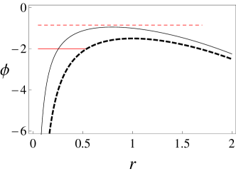
Figure 1: The effective potential $\phi(r)$ versus distance $r$ for $r_{0}=0.05$. Dashed black curve: $\alpha=\beta=1$. Black curve: $\alpha=0.5$, $\beta=1$. The energy $\epsilon=-2$ refers to a bound motion for $\alpha=\beta=1$, but when slowly decreasing $\alpha(t)$ this motion becomes unbounded, i.e. its energy raises above the red-dashed (upper horizontal) line; cf. Fig. 2.

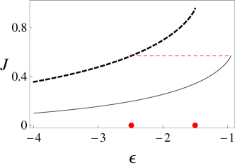
Figure 2: The adiabatic invariant $J(\epsilon)$ as a function of the dimensionless energy $\epsilon$ for $\alpha=\beta=1$ (dashed black curve) and for $\alpha=0.5$, $\beta=1$ (black curve). For both curves $\phi(r_{c})>\epsilon>\phi(r_{0})$, where $\phi(r_{c})$ ($\phi(r_{0})$) is the largest (smallest) energy for the bounded motion. Now energies $\epsilon\in(-1.5,-2.4889)$ (this interval is denoted by two red, bold points) that refer to finite motion under $\alpha=\beta=1$ correspond to infinite motion when $\alpha$ slowly decreases from $\alpha=1$ to $\alpha=0.5$. The range $\epsilon\in(-1.5,-2.4889)$ is additionally illustrated by the horizontal (dashed red) line; cf. Fig. 1.

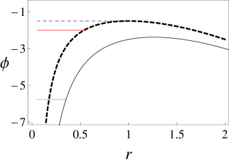
Figure 3: The effective potential $\phi(r)$ versus distance $r$ for $r_{0}=0.05$ [cf. (6)]. Dashed black curve: $\alpha=\beta=1$. Blue dashed line refers to $\phi_{c}=-\frac{3}{2}\alpha^{2/3}\beta^{1/3}$ (for $\alpha=\beta=1$); cf. (7). For all energies below (above) $\phi_{c}$ the motion is bound (unbound). Red line: an example of finite motion at energy $\epsilon=-2$. Black curve: $\phi(r)$ for $\alpha=2$, $\beta=1$. When $\alpha$ slowly changes from $\alpha=1$ to $\alpha=2$, the energy (given initially by the red horizontal line) decreases and always refers to finite motion; for $\alpha=2$ it is given by the green (lower horizontal) line and is equal to $-5.7593$, as found from (12). But if $\alpha$ changes sufficiently fast, the initial energy does not change much an and now it corresponds to an unbound motion; compare red dashed line with the black curve.

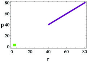
Figure 4: Phase-space density for the inverse parabolic potential with Hamiltonian $H(r,p)=\frac{1}{2}(p^{2}-r^{2})$, where $(r,p)$ are canonically conjugate coordinate and momentum; cf. (13). Green square $[(2,4);(2,4)]$ is the phase-space volume at the initial time $t=0$. Purple figure is the phase-space volume at time $t=3$. The initial volume was filled by $10^{5}$ random points; each point was given a small but finite width, defining a coarse-graining procedure. The evolution of each point was then followed from $t=0$ till $t=3$. It is seen that due to the coarse-graining the phase-space volume increases.

1. Let $M(t)\propto\alpha(t)$ decrease slowly. This can model slow evaporation taking place from the mass $M$. It is now possible that the bounded motion with sufficiently high initial $\epsilon$ becomes unbounded; see Fig. 1. This is related to the fact that (12) does not have solutions $\epsilon_{2}$ for a range of $\epsilon_{1}$ that initially were sufficiently close to $\phi(r_{c})$; see Fig. 2. In other words, during the slow decrease of $\alpha(t)$, $\epsilon(t)$ grows faster than $\phi(r_{c}(t))$. Now it is crucial that the change of $\alpha(t)$ is not very fast; otherwise $\epsilon(t)$ will not change much and will stay bounded. Again $\rho_{V}>0$ is crucial for this scenario. For $\Lambda\leq 0$, the influence of a cyclic change of $\alpha(t)$ on the system can be made arbitrary small, provided that it is sufficiently slow.

2. Let $M(t)\propto\alpha(t)$ increase. This can account for situations with accretion driven increase of $M$. Now $r_{c}$ increases [see (7)] and $\epsilon(t)$ decreases. But if $\alpha(t)$ changes suddenly, $\epsilon(t)$ will not change much and the motion will become unbounded; see Fig. 3. (The energy $\epsilon(t)$ will not change, since during a sudden perturbation the force changes by a finite amount in a small time-interval. Hence the acceleration also changes by a finite amount, while the changes of the coordinate and velocity are negligible; this is the general feature of sudden perturbations.)

Thus, there is a larger class of perturbations such that $\alpha(t)$ changes not slowly, and $\epsilon(t)$ decreases slower than $\phi(r_{c}(t))$; see Fig. 3. Hence it is possible that $\epsilon(t)>\phi(r_{c}(t))$ at some time $t$, and the motion becomes unbounded. This conclusion may seem counter-intuitive: once the mass $M$ increases, the attraction towards the center becomes stronger, but the test particle can escape the attracting center benefiting from the repulsion by the dark energy inside the shell.

It is crucial for this scenario that $\alpha(t)$ increases not slowly. Otherwise, (12) predicts bounded motion; see Fig. 3. This scenario of parametric instability is due to $\rho_{V}\propto\Lambda>0$, e.g. the situation with $\Lambda=0$ (no dark energy) or with $\Lambda<0$ (negative cosmological constant) is stable with respect to this parametric perturbation. Note that when $\alpha(t)$ returns to its initial value—i.e. when the perturbation is over—the motion is not turned back to bounded.

Thus in both scenarios the motion changes from bounded to unbounded. The latter is not ergodic, e.g., only one component of the momentum space is explored. (For example, in the 1d situation the momentum space $P$ has two components $P>0$ and $P<0$.) Similar examples of irreversibility generated by non-ergodicity were analyzed in an .

IV Entropy production

What happens with the test particle once it escapes the bounded part of the potential? The dominant part of potential is now $-\beta r^{2}/2$ and the motion generated by Hamiltonian $H=\frac{1}{2}(p^{2}-\beta r^{2})$,

$$\dot{r}=p,\qquad\dot{p}=\beta r,$$ (13)

is hyperbolic: it has a positive Lyapunov exponent $\sqrt{\beta}\propto\sqrt{\Lambda}$. Due to the second Lyapunov exponent $-\sqrt{\beta}$ it is phase-space volume preserving as any Hamiltonian motion. The exponent $\sqrt{\beta}$ relates to an expanding eigenspace which is also the stable manifold; see Fig. 4. A small coarse-graining will thus lead to an increasing phase-space volume (and thus growing entropy) as demonstrated in Fig. 4. It is expected that the rate of this increase (i.e. entropy production) will be determined by $\sqrt{\beta}\propto\sqrt{\Lambda}$. It was shown that under a weak noise (which is equivalent to a specific coarse-graining) the positive Lyapunov exponent defines the rate of entropy increase for the motion in the inverted parabolic potential paz .

Recall that a coarse-graining (or alternatively an external noise) is standardly needed for getting an arrow of time for a Hamiltonian dynamics gal-or ; lindblad ; balian . Hamiltonian systems displaying the arrow of time are those, where a small coarse-graining leads to entropy increase with a rate that only weakly depends on the coarse-graining gal-or ; lindblad ; balian .

Note that the $\propto\sqrt{\Lambda}$ scaling of the entropy production is natural, since it indicates on the inapplicability of the whole time-arrow scenario for $\Lambda<0$. Indeed, for $\Lambda<0$, the cosmological constant amounts to an overall confining potential and thus increases the stability of the motion.

However, this motion is not chaotic (not even ergodic). It generically does become chaotic provided that its motion becomes bounded at some scale; see fishman for a concrete scenario related to the inverted parabolic potential. It is conceivable that the accelerating particle will meet other masses, and the resulting interaction will achieve an effectively bounded phase-space. Similar and more complex examples of hyperbolic motion in self-gravitating systems were studied in gs ; gk . There is another argument showing that the motion in the inverted-parabolic potential will change its dynamic regime: for a very large $R$ the potential $\Phi(R)$ will assume very large absolute values [cf. (2)], which violates the known applicability condition $|\Phi|/c^{2}\ll 1$ of the non-relativistic description nowak .

It is known that in a Universe with a positive cosmological constant $\Lambda>0$, the long-time evolution of the space-time will be dominated by $\Lambda$ wald . Locally (but not globally) this Universe will look like empty, since the matter will escape through the horizon wald . Now for this Universe it was shown that the generalized second law holds: the sum of the matter entropy and geometric entropy (related to the horizon) does not decrease gib ; davies1 ; davies2 . For very late times, where locally (almost) no matter is present, the matter entropy will tend to zero, while the geometric entropy saturates at a value $\propto 1/\Lambda$ gib ; davies1 ; davies2 . Our consideration concerns the matter entropy and refers to the opposite limit of sufficiently early times, where the matter is abundant, there are bound systems that perform finite motion etc.

V Summary

Thus, the cosmological constant term induces hyperbolicity of motion with the time asymmetry and dynamic entropy production on the large-scale when $\Lambda$ is dominating. We provided a mechanism by which at those scales $\Lambda$ facilitates the thermodynamic arrow. We stress that this mechanism does not directly apply to early universe. Indeed, our starting point is a closed (microcanonically equilibrium) system that does not show an arrow of time before perturbed externally. Such systems exists independently on initial conditions of the early universe.

We also note that the mechanism cannot (and should not) explain all occurences of the thermodynamic arrow. However, note that even when the dark energy (cosmological constant) does not dominate the mean density (early universe or today’s laboratory scale), it still exists. To give an example: for a quantum system in a laboratory $\Lambda$ (= vacuum energy) is not dominating, although it exists (e.g. Casimir effect). Importantly, the dark energy can serve as an ideal thermodynamic bath, since it does not get any back-reaction.

References

- (1) V. Sahni and A. A. Starobinsky, Int. J. Mod. Phys. D, 9, 373 (2000). P.J.E. Peebles and B. Ratra, Rev. Mod. Phys. 75, 559 (2003). E.J. Copeland, M. Sami, S. Tsujikawa, Int. J. Mod. Phys. D15, 1753 (2006).
- (2) Ya.B. Zeldovich, JETP Lett. 6, 883 (1967).
- (3) V.G. Gurzadyan, S.S. Xue, Mod. Phys. Lett. A18, 561, (2003).
- (4) S.G. Djorgovski, V.G. Gurzadyan, Nucl. Phys. B, PS, 173, 6, (2007).
- (5) R. Penrose, Cycles of Time: An Extraordinary New View of the Universe (Bodley Head, London, 2010)
- (6) V.G. Gurzadyan and R. Penrose, Eur. Phys. J. Plus 128, 22 (2013).
- (7) R. Penrose, in General Relativity: An Einstein Centenary Survey ed. S.W. Hawking, W. Israel (Cambridge: Cambridge University Press, 1979).
- (8) H.D. Zeh, The Physical Basis of the Direction of Time, (Springer, Berlin, 1992).
- (9) J.J. Halliwell, J. Perez-Mercader and W.H. Zurek (Eds.) Physical Origins of Time Asymmetry (Cambridge: Cambridge University Press, 1996).
- (10) T. Gold, Amer. J. Phys. 30, 403 (1962). J.E. Hogarth, Proc. Roy. Soc. A 267, 365 (I962).
- (11) E.B. Stuart, B. Gal-Or and A.J. Brainard (Eds.), Critical Review of Thermodynamics (Mono Book Corporation, Baltimore, 1970).
- (12) G. Lindblad, Non-Equilibrium Entropy and Irreversibility, (D. Reidel, Dordrecht, 1983).
- (13) R. Balian, From Microphysics to Macrophysics, volume I, (Springer, 1992).
- (14) G.F.R. Ellis, The arrow of time and the nature of spacetime, arXiv:1302.7291.
- (15) J. Earman, Sharpening the Electromagnetic Arrow(s) of Time, in The Oxford Handbook of Philosophy of Time; edited by C. Callender (Oxford, Oxford University Press, 2011).
- (16) T. Goldman and D. H. Sharp, EPL, 97, 61003 (2012).
- (17) T.D. Lee, Int. J. Mod. Phys. A 16, 3633-3658 (2001).
- (18) A. E. Allahverdyan, R. Balian, Th. M. Nieuwenhuizen, Physics Reports, 525, 1 (2013).
- (19) A. Gomez-Marin, J. M. R. Parrondo, and C. Van den Broeck, EPL, 82, 50002 (2008).
- (20) E. H. Feng and G. E. Crooks, Phys. Rev. Lett. 101, 090602 (2008).
- (21) G. Waldherr and G. Mahler, EPL, 89, 40012 (2010).
- (22) A. Valentini, Physics Letters A 156, 5 (1991).
- (23) Th. M. Nieuwenhuizen, Journal of Physics Conference Series 504, 012008 (2014).
- (24) A.E. Allahverdyan, V.G. Gurzadyan, J. Phys. A: Math. Gen. 35, 7243 (2002).
- (25) V.G. Gurzadyan, A.A. Kocharyan, A & A, 493, L61, (2009); EPL, 86, 29002 (2009).
- (26) V.G. Gurzadyan, P. de Bernardis et al, Mod.Phys.Lett. A20, 813 (2005).
- (27) V.G. Gurzadyan, et al, A & A, 566, A135, (2014).
- (28) I. Szapudi, A. Kovacs et al, MNRAS, 450, 288 (2015).
- (29) P.D. Noerdlinger and V. Petrosian, ApJ, 168, 1 (1971).
- (30) M. Carrera and D. Giulini, Rev. Mod. Phys. 82, 169 (2010).
- (31) A.D. Chernin, Physics-Uspekhi, 51, 253 (2008). M. Eingorn, A. Zhuk, JCAP, 09, 026 (2012). G. W. Gibbons and G. F. R. Ellis, Class. Quant. Grav., 31, 025003 (2014). G. F. R. Ellis and G. W. Gibbons, Class. Quant. Grav., 32, 055001 (2015).
- (32) H. Bacry and J.-M. Levy-Leblond, J. Math. Phys. 9, 1605 (1968).
- (33) V.G. Gurzadyan, The Observatory, 105, 42 (1985).
- (34) W. R. Mason, Philosophical Magazine 14, 386 (1932). E. A. Milne, Quart. J. Math. 5, 64 (1934). W. H. McCrea and E. A. Milne, Quart. J. Math. 5 780 (1934).
- (35) P. A. R. Ade et al, arXiv:1502.01590, (2015)
- (36) A. Balaguera-Antolinez, C. G. Bohmer, and M. Nowakowski, Class. Quant. Grav. 23, 485 (2006).
- (37) A.D. Chernin, Physics-Uspekhi, 56, 704 (2013).
- (38) P. Hertz, Ann. Phys. (Leipzig) 33, 225 (1910); ibid. 33, 537. T. Kasuga, Proc. Jpn. Acad. 37, 366 (1961). E. Ott, Phys. Rev. Lett. 42, 1628 (1979).
- (39) R. Becker, Theory of Heat, (Springer, New York, 1967). V. L. Berdichevsky, Thermodynamics of Chaos and Order, (Addison Wesley Longman, Essex, England, 1997). H.H. Rugh, Phys. Rev. E 64, 055101 (2001).
- (40) L.D. Landau, E.M. Lifshitz, Mechanics (Butterworth-Heinemann, Oxford, UK, 1976).
- (41) A. E. Allahverdyan and Th. M. Nieuwenhuizen, Phys. Rev. E 75, 051124 (2007).
- (42) A. E. Allahverdyan and D. B. Saakian, EPL 81, 30003 (2008).
- (43) W. H. Zurek and J. P. Paz, Phys. Rev. Lett. 72, 2508 (1994).
- (44) A. Cohen and S. Fishman, Int. J. Mod. Phys. B 2, 103 (1988).
- (45) V.G. Gurzadyan and G.K. Savvidy, A & A, 160, 203 (1986).
- (46) V.G. Gurzadyan and A.A. Kocharyan, A & A, 505, 625 (2009).
- (47) M. Nowakowski, Int. J. Mod. Phys. D 10, 649 (2001).
- (48) R.M. Wald, Phys. Rev. D 28, 2118 (1983).
- (49) G.W.Gibbons and S.W. Hawking, Phys. Rev. D 15, 2738 (1977).
- (50) P.C.W. Davies, Phys. Rev. D 30, 737 (1984).
- (51) P.C.W. Davies, Class. Quantum Grav. 4, L225 (1987).