On the calibration of the relation between geometric albedo and polarimetric properties for the asteroids

Abstract

We present a new extensive analysis of the old problem of finding a satisfactory calibration of the relation between the geometric albedo and some measurable polarization properties of the asteroids. To achieve our goals, we use all polarimetric data at our disposal. For the purposes of calibration, we use a limited sample of objects for which we can be confident to know the albedo with good accuracy, according to previous investigations of other authors. We find a new set of updated calibration coefficients for the classical slope - albedo relation, but we generalize our analysis and we consider also alternative possibilities, including the use of other polarimetric parameters, one being proposed here for the first time, and the possibility to exclude from best-fit analyzes the asteroids having low albedos. We also consider a possible parabolic fit of the whole set of data.

1 Introduction

The geometric albedo of a planetary body illuminated by the Sun is the ratio of its brightness observed at zero phase angle (i.e., measured in conditions of ideal solar opposition) to that of an idealized flat, Lambertian disk having the same cross-section. The word “albedo” comes from the Latin word Albus, which means “white”. According to its definition, therefore, the geometric albedo is the parameter used to indicate whether the surface of a given object illuminated by the Sun appears to be dark or bright. The albedo is wavelength dependent. In planetary science, the geometric albedo has been traditionally measured in the standard Johnson $V$ band centered around 0.55 $\mu$m, and it is usually indicated in the literature using the symbol $p_{V}$.

The geometric albedo is a parameter of primary importance. Being an optical property of a sunlight-scattering surface, it must depend on composition, as well as on other properties characterizing the surface at different size scales, including macro- and micro-texture and porosity. All these properties are the product of the overall history of an object’s surface, and are determined by the interplay of phenomena as complex as collisions, local cratering, micro-seismology, space weathering, thermal phenomena, just to mention a few relevant processes. The fine structure and composition of the surface affects properties of the optical emission which determine the results of many observing techniques, including photometry and spectroscopy. It is particularly important in determining the state of polarization of the scattered sunlight in different illumination conditions, this being the main subject of this paper.

The geometric albedo is also a fundamental parameter when one wants to determine the size of a small Solar System body, having at disposal photometric measurements at visible wavelengths. In particular, a measurement of brightness in $V$ light is not sufficient to discriminate between a large, dark object and a small, bright one, if the albedo is unknown.

Geometric albedo should not be confused with the so-called Bond (or spherical) albedo. The Bond albedo is the fraction of incident sunlight that is scattered in all directions and at all wavelengths. The Bond albedo is needed to estimate what fraction of incident radiation is actually absorbed, and therefore contributes to the energy balance of the body determining its temperature. It is possible to define the Bond albedo at any given wavelenght $\lambda$, e.g., $A_{V}$ for that at the V-band of the Johnson UBV system, as $A_{\lambda}=q_{\lambda}\cdot p_{\lambda}$ (Morrison and Lebofsky, 1979), where $p_{\lambda}$ is the geometric albedo at wavelength $\lambda$, and $q_{\lambda}$ is the so-called phase integral, first defined by Russel (1916) as the integral of the directionally scattered flux, integrated over all directions:

$$q_{\lambda}=2\,\int_{0}^{\pi}\Phi(\lambda,\alpha)\sin\alpha d\alpha$$

where $\Phi(\lambda,\alpha)$ is the disk-integrated brightness of the object at phase angle $\alpha$. Unfortunately, a determination of the phase integral, which requires in principle many measurements of the scattered sunlight at visible wavelengths obtained in different illumination conditions, is very hard to achieve, and is seldom available in practice.

Asteroid sizes and albedos have been historically determined mostly by means of measurements of the thermal flux at mid-IR wavelengths (the so-called thermal radiometry technique), generally using space-based platforms like the IRAS and, more recently, the WISE (Masiero et al., 2011) and Akari (Usui et al., 2013) satellites. At thermal IR wavelengths the received flux depends primarily on the size of the emitting object, and only weakly on the albedo. In particular, the Bond albedo determines the fraction of the incident sunlight which is absorbed by the surface and is available to raise the temperature of the body. The temperature, in turn, determines the spectrum of the thermal emission in the IR. Since the Bond albedo of the asteroids is usually fairly low (in general well below $30$%), most of the incident solar flux is actually absorbed by the body, and the intensity of the thermal flux turns out to be mostly dependent on the size, whereas the dependence upon relatively small differences in albedo is much weaker. Moreover, the computation of the geometric albedo from the Bond albedo, as mentioned above, would require a knowledge of the phase integral, which is essentially unknown in the vast majority of cases. As a consequence, it is not really possible to solve simultaneously for size and albedo in practical applications of the thermal radiometry technique. What is normally done is to derive the size from thermal IR data alone (assuming also that the objects have spherical shapes), and then determine the geometric albedo by using the known relation

$$\log(D)=3.1236-0.2H-0.5\log(p_{V})$$ (1)

where $D$ is the diameter expressed in km (supposing that the object is spherical), $H$ is the absolute magnitude and $p_{V}$ is the geometric albedo. To do so properly, at least some $V$ magnitude measurements obtained during the same apparition in which the thermal flux of the object is measured, would be needed, in order to derive from them a reliable value of the absolute magnitude $H$. Unfortunately, in the real world no measurements of the $V$ flux are really done in thermal radiometry campaigns, and $H$ is directly taken from available catalogues. In turn, these $H$ values are derived from $V$ magnitude data (often of quite poor photometric quality), mostly obtained in different observing circumstances, and using a photometric model of the variation of $V$ magnitude as a function of phase angle. As mentioned by several authors, (see, for instance, Muinonen et al., 2010), the magnitude-phase relation for asteroids is described by means of parameters which are generally poorly known, and this introduces further errors in the geometric albedo determination.

In summary, it is difficult to obtain very accurate determinations of the geometric albedo of an asteroid based on thermal radiometry measurements. Based on the relation described by Eq. 1 the relative uncertainty on the albedo should be twice the relative error on the size, in ideal conditions. In practice, values as high as 50 % in geometric albedo, or even more for small and faint objects, are common even when the relative error on the size is of the order of $10$%. The best results require measurements of the thermal flux to be obtained at different wavelengths in the thermal IR, an acceptable knowledge of the variation of $V$ magnitude with phase, and detailed thermo-physical models which can be developed when a wealth of physical data is available from different observing techniques (including a knowledge of the shape and spin axis orientation).

In this paper, we focus on another possible option to obtain estimates of the geometric albedo of asteroids, or other atmosphereless solar system bodies. This is based on measurements of the state of polarization of the sunlight scattered by the surface in different illumination conditions, and on the existence of empirical relations between geometric albedo and polarimetric properties. Our present analysis is mainly devoted to summarize the state of the art of this application of asteroid polarimetry, and to provide one or more updated forms of the albedo - polarization relationship, sufficiently accurate to be used in practical applications of asteroid polarimetry by the largest possible number of researchers in the future. We analyze the current observational evidence taking into account an extensive data set available in the literature, including also observations carried out mostly at the Complejo Astronomico El Leoncito (San Juan, Argentina), that have been published only recently (Gil Hutton et al., 2014). The derivation of the albedo from polarimetric data is a challenging problem which has been open for a long time. In the present paper we take into account both traditional approaches as well as new possible developments suggested by the data at our disposal.

2 Asteroid polarimetric data

Classical asteroid polarimetry consists of measurements of the linear polarization of the light received from asteroids observed at different phase angles. The observations give directly the degree of linear polarization and the position angle of the plane of polarization. This is usually measured with respect to the orientation of the direction perpendicular to the scattering plane, namely the plane containing the Sun, the observer and the target. According to elementary physical considerations (Fresnel reflection) one should expect the scattered sunlight emerging from the surface of an atmosphereless planetary body to be linearly polarized along the direction perpendicular to the scattering plane. This expectation is only partly confirmed by the observations. The asteroid light at visible wavelengths turns out to be, as expected, in a state of partial linear polarization, but in different observing circumstances the plane of linear polarization is found to be either perpendicular (as expected) or parallel (and this is a priori unexpected) to the scattering plane. It is therefore customary in asteroid polarimetry to express the degree of polarization as the ratio of the difference of intensity of light beam component $I_{\perp}$ having the electric vector aligned along the plane perpendicular to the scattering plane minus the intensity $I_{\parallel}$ of the component having the electric vector aligned parallel to that plane, divided by the sum of the two intensities. This parameter is usually indicated as $P_{\rm r}$ in the literature and is given by:

$$P_{\rm r}=\frac{(I_{\perp}-I_{\parallel})}{(I_{\perp}+I_{\parallel})}.$$

According to its definition, the module of $P_{\rm r}$ is the degree of linear polarization of the received light as explained in elementary textbooks in physics (because $I_{\perp}$ and $I_{\parallel}$ are found to be coincident with $I_{\rm max}$ and $I_{\rm min}$ measured through a polaroid), but the sign of $P_{\rm r}$ can be either positive or negative, depending on whether $I_{\rm max}$ corresponds to $I_{\perp}$, as should be expected based on elementary physics, a situation normally referred to as “positive polarization”. When $I_{\rm max}$ is found to correspond to $I_{\parallel}$, $P_{\rm r}$ becomes negative, and this situation is called “negative polarization”.

It is important to note that we will always use the $P_{\rm r}$ parameter throughout this paper every time we will refer to asteroid polarimetric measurements. Its value will always be expressed (and plotted in our figures) in percent (%). We also note that asteroids are not strongly polarized objects. The degree of linear polarization turns out to be usually below $2\%$.

Figure 1: Examples of phase - polarization curves obtained for four large main belt asteroids belonging to different taxonomic classes: top left: the dwarf planet (1) Ceres ($G$-class); top right: (4) Vesta ($V$-class); Bottom left: (6) Hebe ($S$-class); bottom right: (21) Lutetia (for a long time considered to belong to the old $M$ class, now included in the $X$ complex). Open symbols refer to data available in the literature. Full symbols in the plots identify observations obtained at the CASLEO observatory. Most of them have been published only recently (Gil Hutton et al., 2014). The best-fit lines correspond to the exponential-linear relation discussed in Sect. 5.

In asteroid polarimetry, by measuring $P_{\rm r}$ at different epochs, corresponding to different values of the phase angle, it is possible to obtain the so-called phase - polarization curves. Some examples are shown in Fig. 1. Many data plotted in this Figure have been obtained during several observing campaigns carried out at CASLEO (Complejo AStronomico el LEOncito) in the province of San Juan (Argentina), using the 2.15 m Sahade telescope (Gil Hutton et al., 2014). From Fig. 1, it is easy to see that asteroids belonging to very different taxonomic classes tend to exhibit phase - polarization curves which share in general terms a same kind of general morphology, but with differences which can be easily seen, and represent some classical results of asteroid polarimetry (see also Penttila et al., 2005).

In particular, all the curves are characterized by a “negative polarization branch”, extending over an interval of phase angles between $0$ degrees up to a value $\alpha_{0}$ which is commonly found to be around $20^{\circ}$ of phase (“inversion angle”). The extreme value of polarization in the negative branch is traditionally indicated as $P_{\rm min}$. Around the inversion angle the trend of $P_{\rm r}$ as a function of phase angle is mostly linear, and the slope of this linear increase is commonly indicated as $h$. The interval of phase angles which is accessible to Earth-based observers extends in the best cases little over $30^{\circ}$ when observing main belt asteroids (the possible observing circumstances being determined by the orbital elements of the objects). The interval of possible phase angles extends up to much larger values in the case of objects which can be observed much closer to the Earth, as in the case of many near-Earth asteroids.

3 How to calibrate any possible albedo - polarization relation

From Fig. 1, it is evident that, at the same phase angle, different objects exhibit different degrees of polarization. Some objects are more polarized than others. This can be interpreted in very general terms as being a consequence of the classical Umov effect (Umov, 1905), which states that the degree of polarization tends to be inversely proportional to the albedo, according also to laboratory experiments.

The task of determining the albedo based on available phase-polarization curves is important in asteroid science. The foundations have been laid long ago in some classical papers, like Zellner and Gradie (1976) and Zellner et al. (1977). Since then, several authors have tackled the same problem, with analyzes based on new sets of observations and/or laboratory experiments. The idea is to determine some suitable relation between the distinctive features of the phase - polarization curves of some selected sources, and their albedo, assumed to be known a priori with good accuracy. The set of calibration objects must also be representative of the whole population.

We cannot assume a priori that all asteroids (which are a quite heterogeneous population), must respect a unique relation between albedo and polarization properties. Only a posteriori can we assess whether it is possible to accurately derive the albedo using a unique relationship independent on the taxonomic class. The main task is therefore to find a suitable representation of such a relation between albedo and polarization, to be tested over the maximum possible number of calibration objects belonging to different taxonomic classes.

In this respect, one must analyze available polarimetric data for the largest possible sample of objects having a well-known albedo, in order to find evidence of some general and satisfactorily accurate relation between albedo and polarimetric properties. Unfortunately, it is not so easy to implement this simple approach in practical terms. The use of laboratory experiments, based in particular on polarimetric measurements of meteorite samples, for calibration purposes seems to be natural, and was adopted in the 70s, but it is not exempt from problems. There are some technical difficulties, including the need of observing the specimens at zero phase angle to measure their albedos, something which is in general not a trivial task. In a classical paper, Zellner et al. (1977) also mentioned some problems in correctly assessing the instrumental polarization in the lab. Another general problem is to ensure that the used meteorite samples are really representative of the behavior of asteroids as they appear to remote observers. Unfortunately, the meteorite samples have to be treated to reproduce the texture of their asteroid parent bodies. For instance, Zellner et al. (1977) noted that to find similarities between the phase-polarization curves of asteroids and meteorite samples, the latter have to be first crushed, and the way to do that has consequences on the derived polarization properties. Moreover, the authors noticed how difficult it is to eliminate from meteorite samples any source of terrestrial, post-impact alteration. For all these reasons, starting from the 90s most attempts of calibration of the albedo - polarization relation have been based on the direct use of asteroid albedo values obtained from other techniques of remote observation.

Several papers have been based on the idea of using for calibration purposes some sets of asteroids for which the geometric albedo had been derived from thermal radiometry observations, mostly consisting of old IRAS measurements, or, more recently, WISE data. This approach has the advantage of being able to use for calibration many objects belonging to practically all known taxonomic classes. There are, however, several problems. First, albedos derived from thermal IR data are model-dependent. They depend on the choice of some parameters, which are needed to simulate the distribution of temperature on the asteroid surface, and the dependence of the irradiated thermal flux in different directions. Apart from a limited number of cases, albedo values determined by thermal radiometry data, particularly for objects for which we have little information coming from other sources, are simply too inaccurate for the purposes of a robust calibration. This is a consequence of the problems discussed in Section 1 concerning the general lack of simultaneous photometric data at visible wavelengths, and the consequent use of values of absolute magnitude that are affected by large errors. To add some confusion, in the past the catalog of IRAS-based asteroid albedos changed with time. In particular, the first published catalog of IRAS albedo values (Tedesco and Veeder, 1992) had been built using thermal IR data coupled with estimated absolute magnitudes computed prior the introduction of the ($H$, $G$) asteroid photometric system. Using these data, Lupishko and Mohamed (1996) derived a first set of values for the calibration parameters included in the so-called slope-albedo law (see Section 4). Subsequently, a new IRAS albedo catalog was produced using absolute magnitudes expressed in the ($H$, $G$) system (Tedesco et al., 2002), and these values were used by Cellino et al. (1999) to derive an alternative calibration of the slope-albedo law. This problem should be expected to arise again, due to the fact that IAU has recently recommended the use of a new photometric system ($H,G_{1},G_{2}$, see Muinonen et al., 2010), implying that the albedo catalogues obtained using IRAS, and more recently, WISE data, should be updated again.

Currently, different authors use different calibrations available in the literature, including, in addition to those just mentioned above, also much older calibrations by Zellner et al. (1974) and Zellner et al. (1977), which were mainly based on laboratory experiments. This is not an ideal situation, and one of the major goals of this paper is just to provide one or more updated forms of the albedo - polarization relationship, to be used by most researchers in the future, depending on the polarimetric data at their disposal.

Masiero et al. (2012) proposed a new kind of calibration based on different polarimetric parameters and using a sample of $177$ asteroids for which the albedo has been estimated from WISE thermal radiometry data. In many cases, the objects were observed by WISE at fairly large phase angles, and the problem of assigning in these cases reliable values of corresponding magnitude in the visible is particularly difficult. As a consequence, in this paper we will also make a new test of the Masiero et al. (2012) approach, but using a different sample of objects having albedos not derived from thermal radiometry data (see Section 6).

Shevchenko and Tedesco (2006) proposed to use for calibration purposes a limited sample of asteroids for which both the size is known with extremely high accuracy, and also the absolute magnitude in the visible is well known, being based on large data sets of available photometric data. As for the size, the most accurate values are certainly those obtained either in situ by space probes, or those obtained by accurate observations of stellar occultations. At least for some of these objects, also the absolute magnitude values listed in the catalogs can be reasonably reliable, although we should always remember that the absolute magnitude is not, strictly speaking, a fixed parameter, but it varies at different epochs, being dependent on the varying aspect angle of the object. The aspect angle determines the extent of the cross-section of the illuminated surface visible by the observer, and varies at different apparitions. This variation of visible cross-section depends on the overall shape of the object (it is zero for an ideal sphere) and on the orientation of the rotation axis.

Limiting our analysis to the best-observed objects, for which the size and the absolute magnitude are supposed to be well known, the albedo $p_{V}$ can be derived using the relation between size, albedo and absolute magnitude (Eq. 1)

The list of objects with reliable albedo proposed by Shevchenko and Tedesco (2006) includes $61$ objects. Among them, there are some of the largest and most observed asteroids, including (1) Ceres, (2) Pallas, (3) Juno and (4) Vesta. We note that in the case of (4) Vesta, however, we use a different value of albedo, namely $0.35\pm 0.02$, based on the most recent, and very accurate value of size measured in situ by the Dawn probe. The uncertainty in albedo for this asteroid depends on the fact that the disk-integrated albedo tends to change at different rotation angles (Cellino et al., 2015). Many objects of the Shevchenko and Tedesco (2006) list are much fainter (including some small targets of space missions) and several have never been observed in polarimetry. In this paper we follow the approach indicated by Shevchenko and Tedesco (2006). This does not mean that we are not aware of some problems: first, we know that the Shevchenko and Tedesco (2006) object list is now fairly old and needs an updating. This includes both considering a larger, currently available set of high-quality stellar occultation data, as well as using more accurate values of the absolute magnitude, to be computed according to the new ($H$, $G_{1}$, $G_{2}$) photometric system adopted by the International Astronomical Union. We plan to produce an updated and possibly longer list of calibration targets in the near future, but we postpone this to a separate paper. In our present work we lay the foundations for any future analysis taking profit of a larger list of reliable asteroid albedos. The still limited data base of asteroid polarimetric observations is for the moment the main limiting factor for the investigations in this field.

We have long been involved in an observing program of polarimetric observations of asteroids belonging to the Shevchenko and Tedesco (2006) list, in order to improve significantly the coverage of the phase-polarization curves for these objects. So far, we have been able to obtain decent phase-polarization curves for only a limited sample of the whole list, taking also into account that some objects would require the availability of larger telescopes and/or better detectors, as well as a larger amount of dedicated observing time. The results presented in this paper, which follow a previous preliminary analysis published by (Cellino et al., 2012), are already sufficient to find an updated set of calibration parameters for the classical form of the slope-albedo law adopted by most authors in the past. The new data also allow us to explore new possible ways to express the relation between albedo and polarimetric properties, which will be probably the future in this field once the data-set of asteroid polarimetric measurements will grow significantly in a hopefully not-too distant future.

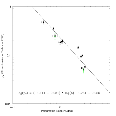
Figure 2: The slope-albedo relation, in log-log scale, for $15$ asteroids of the list of Shevchenko and Tedesco (2006) for which a computation of the polarimetric slope is possible based on measurements obtained so far. Objects for which we have at disposal at least $10$ polarimetric measurements are indicated by full, black symbols. Objects having a number of observations between $5$ and $10$ are displayed using open, green symbols. The obtained polarimetric slopes of all the objects in this plot have been used in the computation of the linear best-fit that is plotted together with the individual data. The corresponding values of the $C_{1}$ and $C_{2}$ calibration coefficients are also indicated.

4 The classical approach: the slope-albedo “law”

In practically all papers devoted in the past to this subject, the relation between geometric albedo and polarimetric properties has been assumed to be one of the following ones:

$$\log(p_{V})=C_{1}\log(h)+C_{2}$$ (2)

$$\log(p_{V})=C_{3}\log(P_{\rm min})+C_{4}$$ (3)

In Eq. (2), which was originally proposed as early as in the 70s in the first pioneering investigations by B. Zellner and coworkers, $h$ is the so-called polarimetric slope, namely the slope of the linear variation of $P_{\rm r}$ as a function of phase angle, measured at the inversion angle (see Section 2). In Eq. (3), the polarimetric parameter is instead $P_{\rm min}$, namely the extreme value of negative polarization.

Most investigations available in the literature (see, for instance, Cellino et al., 2012, and references therein), have used Eq. (2), which is normally known as the slope - albedo relation, or law. In fact, according to many authors, Eq. 3 leads to less (or much less) accurate results than Eq. 2. We will come back to this point in Section 5, while in the rest of this Section we will focus on Eq. 2.

The measurement of the polarimetric slope $h$ should be done, in principle, by measuring the degree of linear polarization $P_{\rm r}$ in a narrow interval of phase angles surrounding the inversion angle. In practical terms, however, the observers rarely have at disposal an ideal coverage of the phase - polarization curve, and often the polarimetric slope is derived by making a linear fit of a few $P_{\rm r}$ measurements, located not so close to the inversion angle as one would generally hope. We will see in the next Sections some new possible approach to derive $h$ when one has at disposal a good coverage of the phase - polarization curve. For the moment, however, in a first treatment of available polarimetric data for the objects of the Shevchenko and Tedesco (2006) list, we adopt the usual techniques, and we derive $h$ from a linear least-squares fit of all available $P_{\rm r}$ data. In particular, in order to use only homogeneous and high-quality data:

• We limit our analysis to polarimetric measurements obtained in the standard $V$ filter.

• we only use values of linear polarization $P_{\rm r}$ having nominal errors less than $0.2$%.

• We use only polarimetric measurements obtained at phase angles larger than or equal to $14^{\circ}$ of phase, a value generally well beyond the phase corresponding to $P_{\rm min}$, and in a region of the negative polarization branch where $P_{\rm r}$ starts to increase linearly with phase.

• We require to have at least $5$ accepted measurements, and that the interval of phase angles covered by the data is not less than $3^{\circ}$.

A smaller number of measurements, and a narrower interval of covered phase angles, would make the adopted polarimetric slopes more uncertain. The use of $P_{\rm r}$ data having fairly large error bars, up to 0.2, is suggested by the general scarcity of polarimetric data, but the effect of low-quality measurements is mitigated because in the computation of the best-fit curves, we weight the data according to the inverse of the square of their associated errors. As for the nominal errors of the Shevchenko and Tedesco (2006) albedos, which are not explicitly listed by the authors, we derived them using the quality codes listed in the above paper, according to their meaning as indicated by the authors.

In this way, we were able to compute reliable polarimetric slopes for $15$ calibration objects. Taking the corresponding albedos from the Shevchenko and Tedesco (2006) paper, we can plot $h$ as a function of albedo, in a log-log scale, from which the coefficients $C_{1}$ and $C_{2}$ in Eq. (2) can be derived using simple least-squares computations. The nominal errors of both the calibration albedos and of the derived polarization slopes were taken into account in the computation.

The results, including also the obtained values of the $C_{1}$ and $C_{2}$ calibration parameters, are shown in Fig. 2. The values of $C_{1}$ and $C_{2}$, together with their corresponding errors, are also given in Table 1. A few considerations are suggested by looking at Fig. 2. First, the linear best-fit solution seems, as a first approximation, fairly reasonable.

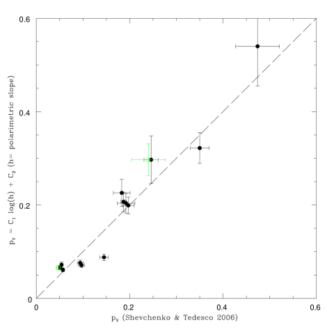
Figure 3: Comparison between the albedos of $15$ objects observed in our campaign, derived using our new calibration coefficients of the slope-albedo relation, and the corresponding albedo values given by Shevchenko and Tedesco (2006). The meaning of the symbols is the same as in Fig. 2

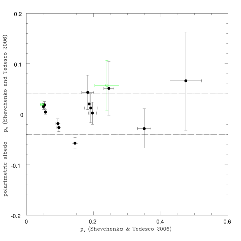
Figure 4: Plot of the difference between the albedo values derived using the new calibration coefficients of the slope-albedo relation for objects included in the Shevchenko and Tedesco (2006) list and the corresponding values found by the above authors. The dashed lines correspond to differences of $\pm 0.04$ in albedo. The meaning of the symbols is the same as in Fig. 2.

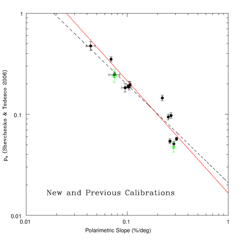
Figure 5: A comparison between the calibration of the slope-albedo relation presented in this paper (red line) and those by Cellino et al. (2012) (black, dashed line).

This seems to be confirmed by Figure 3, where the albedo values of the objects considered in our analysis, as they can be derived from our updated determination of the calibration coefficients, are plotted versus the corresponding albedo values determined by Shevchenko and Tedesco (2006). In Fig. 4 we show for each object the difference between the albedo value obtained from the polarimetric slope and the albedo value given by Shevchenko and Tedesco (2006). From Figs. 2 to 4, it can be seen that the discrepancies are generally low in absolute terms, being mostly below $\pm 0.04$, as shown in Fig. 4. The error bars of the obtained albedo values tend to increase with albedo, but this should be expected, because the slope-albedo relation (Eq. 2) implies that the error of $p_{V}$ must increase linearly with $p_{V}$ itself.

One object turns out to have a polarimetrically-derived albedo that is significantly discrepant, namely (2) Pallas, (the point which is located at the highest vertical distance above the best-fit line in Fig. 2). The Shevchenko and Tedesco (2006) albedo value of this asteroid, $0.145$, seems to be noticeably high for an object belonging to the $B$ taxonomic class, which is generally supposed to include low-albedo asteroids. On the other hand, the Shevchenko and Tedesco (2006) albedo of Pallas is also substantially confirmed by more recent results based on WISE data (Masiero et al., 2011). The albedo value derived from the polarimetric slope turns out to be $0.088\pm 0.007$, which would appear to be more in agreement with expectations for a body belonging to the low-albedo, $B$ class. It is interesting to note that De Leon et al. (2012) observed a large sample of $B$-class objects and found a continuous variation of near-IR spectral slopes, possibly suggesting a variety of different compositions. This might be a consequence of the fact that the modern $B$ class includes also some asteroids (the old $F$ class of Tholen, see Tholen and Barucci, 1989) that in the 80s were kept separate based on their behaviour at the shortest wavelengths, which are no longer covered in the most modern spectroscopic investigations. One should also take into account that the surface properties of the largest asteroids like (2) Pallas, which retain a larger fraction of the material excavated in most impacts, can be different from those of smaller asteroids which lose a much larger fraction of the impact debris from most collisions to space. We already know, based on their different IR beaming parameters, that the surfaces of large and smaller asteroids can be significantly different. In any case, polarimetry seems to indicate for (2) Pallas a low albedo. In the absence of any new, updated albedo and/or absolute magnitude value for this object coming from other sources, we accept this discrepancy.

Another important problem which is most apparent in Fig. 3 concerns the asteroid (64) Angelina, namely the object having the highest albedo value in our sample. The value given by Shevchenko and Tedesco (2006) for this object is $0.474\pm 0.047$. According to our new calibration, the resulting albedo turns out to be $0.540\pm 0.085$, marginally in agreement with the Shevchenko and Tedesco (2006) value. The problem here is not this discrepancy per se, but rather the fact that, as shown in Fig. 2, in the high-albedo domain our new calibration tends to assign albedo values increasingly close to $1.0$ to asteroids having increasingly shallower polarimetric slopes.

In Fig. 5 we show a comparison between our new slope-albedo relation (shown in red in the plot) and the most recent previous calibration, namely that of Cellino et al. (2012) (black line). Though not being visually very different, an effect of the adopted log-log scale, the new calibration tends, at high values of albedo, to stay well above the values predicted by the previous calibration. We will show in a separate paper that in the case of (44) Nysa, an asteroid belonging to the high-albedo $E$ class, our new calibration assigns to this asteroid an albedo of about $0.9$, which seems exceedingly high to be credible for a rocky body. In the domain of low-albedo asteroids, the larger steepness of the new best-fit line produces only a marginally better fit with respect to the previous calibration.

This problem of an exceedingly high slope of our linear calibration seems to be connected with another major problem that is apparent by looking at Fig. 2. This is the fact that at low albedo, the data look rather noisy, with some data points, having polarimetric slopes between $0.2$%/deg and $0.3$ %/deg, which are located well above or below the linear best-fit of the whole dataset. Trying to fit all the data, one is led to accept a linear best-fit whose steepness is a consequence of the presence of the lowest-albedo asteroids. This is a problem that has been known since a long time, and we will discuss it more extensively in the following Subsection.

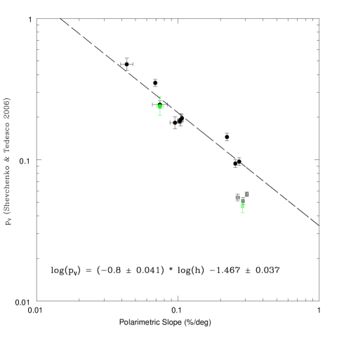
Figure 6: The same as Fig. 2, but here the objects having albedo smaller than $0.08$ (displayed here using open squares) were not used to derive the displayed linear best-fit. The corresponding values of the $C_{1}$ and $C_{2}$ calibration coefficients are also indicated.

4.1 Effects of excluding low-albedo objects

In general terms, looking at Fig. 2, one could be tempted to conclude that it is hard to fit the whole dataset by using one unique linear relation. In particular, it may appear that, if one could drop a handful of objects having albedo lower than about $0.08$, one could obtain a much better fit for the remaining objects. This is an old-debated subject, namely whether there is evidence of a saturation of the slope -albedo law at small albedo values. This kind of possible saturation is also much more evident in $P_{\rm min}$ - albedo data, as we will see in Section 5.

What happens if we exlude from our analysis low-albedo asteroids? Figure 6 shows the results of this exercise. As expected, the RMS deviation of the linear best-fit of the data, which is now much shallower than in the case in which we kept all the available measurements, is quite better, as shown in Table 4. One could conclude that excluding the asteroids having albedo lower than $0.08$ is the best way to proceed to obtain an improved, and quite better, calibration of the slope - albedo law. Figure 7 shows that in this way, the relative error on the derived albedo values turns out to be generally better than $20$%, a quite good result.

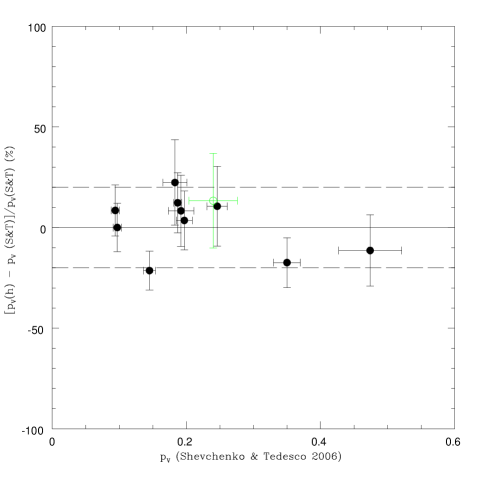
Figure 7: The same as Fig. 4, but here the objects having albedo smaller than $0.08$ are not included in the analysis, and the plot shows the relative error of the albedo determinations.

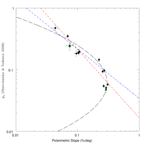
Figure 8: Results of a parabolic best-fit of all available slope - albedo data. The corresponding linear fits shown in Fig. 2 and in Fig. 6 are also displayed for a comparison (red and blue dashed lines, respectively).

The problem, of course, is that in the practical applications of asteroid polarimetry, one has at disposal the polarimetric slope derived from observations, and wants to derive from it the albedo, which is unknown. Unfortunately, there is a range of values of polarization slope which is shared by objects having albedo either around $0.05$ or around $0.10$. By using a slope - albedo relation which is not valid for low-albedo asteroids may produce a systematic overestimate of the albedo for dark objects.

The best procedure to be adopted in practice may be the following: when the polarimetric slope of an object is measured with good accuracy, it will be better to use the calibration coefficients obtained by dropping low-albedo objects, displayed in Table 1 and Fig. 6, but only when the polarimetric slope turns out to be smaller than about $0.25$%/deg. In this way, the relative error in the determination of the albedo should be within $20$%, a nice result, as shown in Fig. 7.

If the slope is larger than the above value, and/or when the value of polarization slope is more uncertain, the best choice would be probably to use the calibration coefficients fitting the whole population, displayed in Table 1 and Fig. 2. The errors that one should expect for the higher values of polarimetric slopes should be in any case limited, of the order of about $\pm 0.03$, not negligible in relative terms, but in any case sufficient to correctly classify the objects as low-albedo asteroids.

The polarimetric slope data shown in Fig. 2, can also suggest that a linear fit is not fully adequate to represent the whole dataset, and a parabolic fit could be more suited to better represent the data. This is shown in Fig. 8, in which a parabolic relation

$$\log(h)=H_{1}(\log(p_{V}))^{2}+H_{2}\log(p_{V})+H_{3}$$

is adopted, and the result of a best-fit procedure is shown. The linear plots already shown in Fig. 2 and Fig. 6 are also shown for a visual comparison. It is clear from the Figure that a parabolic fit applied to the whole dataset gives good results. The slightly worse fit of some objects having albedo around $0.2$ (located below the parabolic fit) seems to be compensated by a much better fit of the polarimetric slope and albedo of the asteroid (2) Pallas, which is the most discrepant object when trying linear fits to represent the data. However, there is still the problem of the ambiguity affecting the values of albedo to be assigned to objects having polarimetric slopes between $0.2$%/deg and $0.3$%/deg, which cannot be solved.

For this reason, we list the obtained values of the $A$, $B$, $C$ coefficients of our parabolic fit in Table 1, but we are not claiming that there is such a big improvement with respect to the classical linear fit, specially when dropping the lowest-albedo objects, to force us to necessarily use a parabolic fit in the future. Things could change in the case that the discovery of other objects sharing the location of (2) Pallas in the $h$ - $p_{V}$ plane would confirm that a linear fit is not really suited to adequately represent them, even by excluding from the analysis low-albedo objects. Another possibility is that future theoretical advances in the interpretation of light scattering phenomena could suggest that a parabolic fit is intrinsically more correct to fit the relation between polarimetric slope and geometric albedo, based on some physical arguments.

5 More on classical approaches: fitting phase-polarization curves

One can wonder whether the slope - albedo relation is really the best available choice to derive good estimates of asteroid albedos. In fact, asteroid phase - polarization curves do not include only the (mostly) linear variation of $P_{\rm r}$ around the inversion angle. A negative polarization branch also exists, not to mention the behavior exhibited at large phase angles (not achievable for main belt objects) by near-Earth asteroids.

Historically, another relation between albedo and polarization properties was found to involve the $P_{\rm min}$ parameter, as shown in Eq. (3). As mentioned in the previous Section, this has been generally abandoned in recent years, because $P_{\rm min}$ data have been found by some authors to be quite scattered around the best-fit representation given by Eq. 3. On the other hand, one could also wonder whether this might be at least partly a consequence of the difficulty of deriving accurate values of $P_{\rm min}$ from the observations, making use of visual extrapolations of rather sparse polarimetric data. This leads us to face the problem of finding suitable analytical representations of the morphology of phase - polarization curves.

Figure 9: The values of the best-fit parameters $A$ and $B$ found for the best 200 solutions of the linear-exponential relation applied to polarimetric data of asteroid (216) Kleopatra, using a “genetic” algorithm. Note that all the plotted solutions for $A$ and $B$ give nearly identical residuals and produce best-fit curves characterized by values of $h$, $P_{\rm min}$ and other polarimetric parameters which are essentially identical (within the nominal error bars).

Figure 10: The same as in Fig. 9, but for the $A$ and $C$ parameters in Eq. 4.

In this paper we follow the example of previous authors, and we use the following exponential-linear relation:

$$P_{\rm r}=A(e^{-\alpha/B}-1)+C\cdot\alpha$$ (4)

where $\alpha$ is the phase angle expressed in degrees, and $A$, $B$, $C$ are parameters to be determined by means of best-fit techniques. This analytical representation has been found in the past to be suited to fit both phase - magnitude relations in asteroid photometry, and phase - polarization curves in asteroid polarimetry (Kaasalainen et al., 2003; Muinonen et al., 2009). Some examples of practical applications of the above relation are the best-fit curves of the phase-polarization curves of the asteroids shown in Fig. 1. According to its mathematical representation, when the parameters $A,B,C$ are all positive, the exponential-linear relation describes a curve characterized by a negative polarization branch between $0$ and an inversion angle $\alpha_{\rm inv}$. The trend tends to become essentially linear at large phase angles, where the exponential term tends quickly to zero.

The computation of the best-fit representation of any phase-polarization curve using Eq. 4 can be done in many ways. In the present paper, we use a genetic algorithm, which, starting from a random set of $A,B,C$ values, explores the space of possible solution parameters and finds the set of $A,B,C$ values producing the smallest possible residuals. Due to the intrinsic properties of a genetic approach, the algorithm is launched several times, in order to have a correspondingly high number of solutions, in order to ensure that we are not missing the best possible one.

It should be noted, however, that the evaluation of the errors of any polarimetric parameter derived by a best-fit of the phase - polarization curve using Eq. 4, is complicated by the fact that the parameters $A$, $B$ and $C$ that minimise the $\chi^{2}$ are correlated. To illustrate this situation, Fig. 9 shows that different pairs of $A$ and $B$ values produce fits nearly indistinguishable in terms of r.m.s. residuals (the differences being not larger than 0.0015). Figure 10 shows a similar situation for the parameters $A$ and $C$. This means that the non diagonal elements of the error matrix (see, e.g., Bevington, 1969) are not negligible with respect to the diagonal ones, and therefore the calculation of the error on any polarimetric parameter derived from the exponential-linear curve should take into account all the various co-variances. Our method for the $\chi^{2}$ minimization is based on a genetic algorithm, which does not produce automatically the error matrix. For the estimate of the error on polarimetric parameters derived by best-fit values of $A,B,C$, it is therefore more practical to adopt an alternative method. Let us assume, as an example, that we are interested in determining $P_{\rm min}$ and its corresponding uncertainty. The resulting value of $P_{\rm min}$ will be the one obtained using the $A,B,C$ values giving the smallest $\chi^{2}$. As for the error to be assigned to this determination of $P_{\rm min}$, the method that we adopt consists of calculating all $P_{\rm min}$ values corresponding to identified sets of $A,B,C$ parameters that produce a fit of the phase - polarization curve giving $\chi^{2}$ values such that $\chi^{2}\leq\chi^{2}_{\rm min}+1$. We then define as error on $P_{\rm min}$ the half difference between the extremes of the various $P_{\rm min}$ values so obtained. This approach was followed e.g. by Bagnulo et al. (1995) and is consistent with the error analysis presented by Bevington (1969). Needless to say, this procedure may be applied to the determination of any polarimetric parameter (other than $P_{\rm min}$) derived by an exponential-linear fit of the phase-polarization curve.

In what follows, since we want to limit our analysis only to high-quality and well-covered phase - polarization curves, we impose some strict constraints on the selection of the objects for which we compute a best-fit using the exponential-linear relation. In particular:

• we exclude a priori from our analysis all measurements having a nominal accuracy of $P_{\rm r}$ worse than $0.20$.

• we require to have at least $4$ accepted measurements taken at phase angles $>2^{\circ}$.

• we require to have at least $1$ accepted measurement taken at phase angles $\geq 17^{\circ}$.

• we require to have at least $1$ accepted measurement taken at phase angles $<14^{\circ}$.

• we require to have at least $3$ accepted measurements taken at phase angles $<30^{\circ}$.

As in the case of the computation of the polarimetric slope described in the previous Section, we limit our analysis to available data obtained in $V$ filter. Here, however, we add an additional constraint: we do not use for calibration purposes the best-fit phase - polarization curves of asteroids for which we have fewer than $10$ accepted $P_{\rm r}$ measurements. All the criteria described above are dictated by our will to restrict our calibration procedures to the objects having excellently determined and optimally sampled phase - polarization curves, only.

5.1 Use of $P_{\rm min}$

Having at disposal a best-fit representation of a phase-polarization curve according to Eq. 4, one can compute the resulting $P_{\rm min}$ value and the corresponding phase angle $\alpha(P_{\rm min})$ at which it is found. More in detail, $\alpha(P_{\rm min})$ can be computed by equaling to zero the first derivative of Eq. 4, from which we obtain:

$$\alpha(P_{\rm min})=\ln(\frac{A}{BC})$$

then, $P_{\rm min}$ can be computed as $P_{\rm r}(\alpha(P_{\rm min}))$ using Eq. 4. The nominal uncertainty in $P_{\rm min}$ has to be computed by doing a formal propagation of the errors of the $A,B,C$ parameters found in the best-fit solution of xEq. 4, using the procedure explained above.

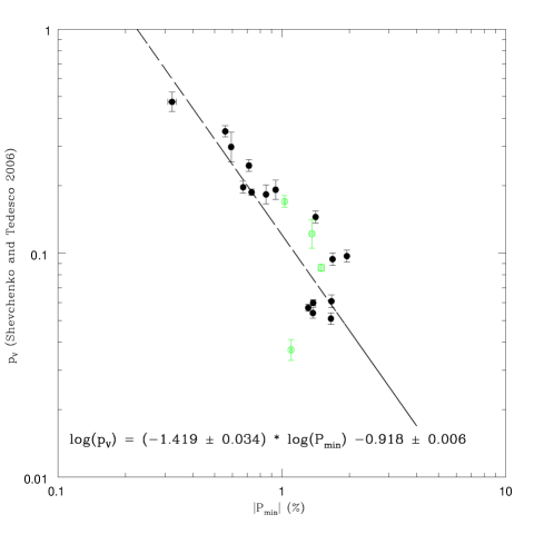
Figure 11: Best-fit relation between $P_{\rm min}$ and geometric albedo for an available sample of $20$ asteroid targets included in the Shevchenko and Tedesco (2006) list. Only $16$ objects for which we have at disposal at least ten polarimetric measurements have been used to derive the best-fit solution. These objects are plotted as full, black symbols. Open, green symbols represent objects for which we have fewer than ten observations, and were not used in the least-squares computation.

In the case of the $P_{\rm min}$ - albedo relation described by Eq. 3, the results of our exercise are shown in Fig. 11, including the best-fit values we find for the $C_{3}$ and $C_{4}$ coefficients. The calibration is based on data of the $P_{\rm min}$ values of $16$ objects belonging to the Shevchenko and Tedesco (2006) list, for which we have at least $10$ polarimetric measurements. Four additional asteroids, for which we have fewer than ten measurements, are also shown using different symbols, but they were not used in the computation of the best-fit. The obtained values of $C_{3}$ and $C_{4}$ calibration coefficients, together with their corresponding errors, are also given in Table 1. We see that, not unexpectedly, the distribution of the points in the $P_{\rm min}$ - albedo plane, in our log-log plot (in Fig.11) makes it difficult to find a satisfactory linear fit. Correspondingly, the agreement of the resulting albedos with those of the Shevchenko and Tedesco (2006) list is significantly worse than in the case of the calibration based on the polarimetric slope. As shown in Table 3, we find a large discrepancy in the case of the bright asteroid (64) Angelina, for which a very high value of albedo of $0.600\pm 0.044$ is obtained from the $P_{\rm min}$ - albedo relation, much larger than the $0.474\pm 0.047$ value listed by Shevchenko and Tedesco (2006). The majority of the other asteroids of our sample, conversely, tends to have an albedo underestimated with respect to the calibration values, apart from a few ones having the lowest albedo values. Among them, we note the difference between the very low albedo value found by Shevchenko and Tedesco (2006) for asteroid (444) Gyptis ($0.037\pm 0.004$) and the value of $0.106\pm 0.002$ that we obtain from its $P_{\rm min}$ value. This object, however, was not used in the derivation of the best-fit computation, because only $6$ polarimetric measurements are currently available for it, and moreover the phase - polarization curve (not shown) is quite noisy. We note also that the albedo value found by Shevchenko and Tedesco (2006) is very low, and might possibly be slightly underestimated.

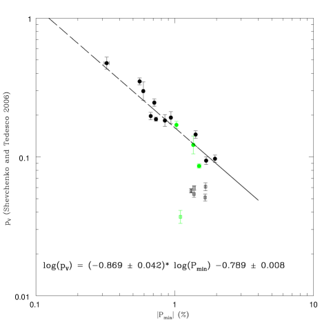
Figure 12: The same as Fig. 11, but here the objects having albedo lower than $0.08$ (sowed using open symbols) were not used in the computation of the linear best-fit.

By simply looking at Fig.11, a saturation of the $P_{\rm min}$ - albedo relation at low albedo values is even more evident than in the case of the slope - albedo relation analyzed in Section 4.1. It seems therefore that a removal of asteroids having albedo less than about $0.08$ from the best-fit computation is even more justified in this case. The result of this exercise is shown in Fig. 12. The improvement of the residuals, listed in Table 4, is very important, as also visually shown in the Figure.

The big improvement of the obtained best-fit makes this $P_{\rm min}$ - albedo relation much more suitable for the determination of the albedo, but, again, this refers to only a more limited interval of possible $P_{\rm min}$ values, in particular those lower (in absolute value) than about $1$%. For objects having deeper $P_{\rm min}$, the corresponding interval of possible albedo values is exceedingly wide to be used to derive a useful albedo determination. Based on our results, we confirm therefore that, in general, the use of $P_{\rm min}$ as a reliable diagnostic of the albedo, but for asteroids exhibiting a shallow polarization branch, should not be encouraged.

5.2 An alternative derivation of the polarimetric slope

Using the global fitting of the phase polarization curves given by Eq. 4, it is also possible to modify the way to derive the polarimetric slope $h$. In so doing, one can make use of all the available polarimetric measurements, and not only of those obtained in a more or less narrow interval of phase angles centered around the inversion angle. In particular, the polarimetric slope can be determined as the first derivative of $P_{\rm r}$ with respect to the phase angle (using Eq. 4), where the derivative has to be computed at the inversion angle $\alpha_{\rm inv}$. In turn, the value of $\alpha_{\rm inv}$ can also be derived with excellent accuracy from Eq. 4. We adopt here a very simple numerical approach. Having determined the values of parameters $A$, $B$, $C$ corresponding to the nominal best-fit solution, we make an iterative computation of $P_{\rm r}$  starting from an initial phase angle value of $1$ degree, and using a fixed increment of $+0.02$ deg in phase. When $P_{\rm r}(i+1)\cdot P_{\rm r}(i)$ becomes negative, we consider that $\alpha_{inv}$ is equal to $P_{\rm r}(i)+0.01$ degrees, with an uncertainty of $0.02$ degrees.

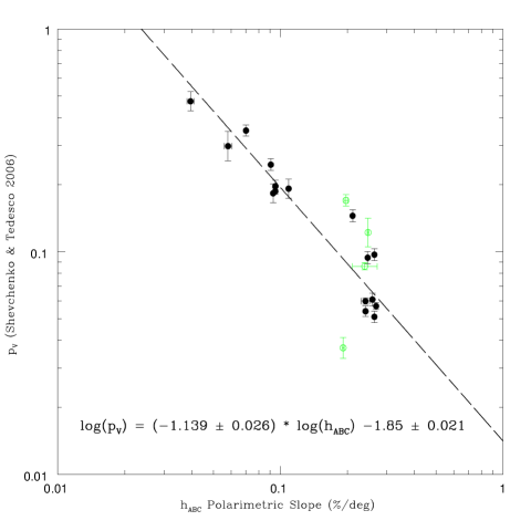
Figure 13: The same as Fig. 2, but here the polarimetric slope $h_{ABC}$ is computed as the first derivative of $P_{\rm r}$ (according to Eq. 4) at the inversion angle $\alpha_{inv}$ for $20$ asteroids of the Shevchenko and Tedesco (2006) list. Four objects having fewer than ten polarimetric measurements were not used for the computation of the best-fit. They are indicated by open, green symbols.

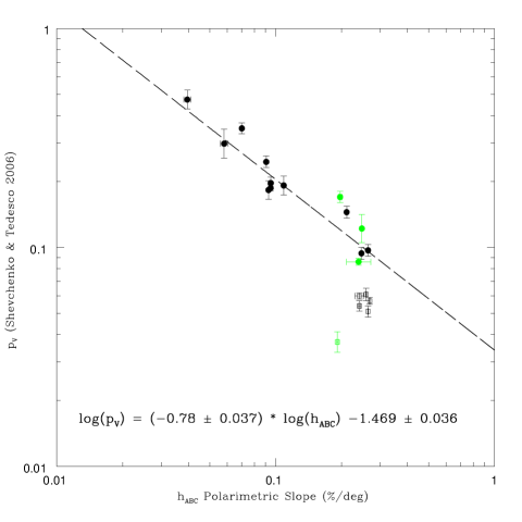
Figure 14: The same as Fig. 13, but here objects having an albedo lower than $0.08$ (shown using open squares) are not used in the computation of the best-fit.

Having determined the inversion angle, we can compute the resulting polarimetric slope as the first derivative of Eq. 4, using the same procedure already adopted for $P_{\rm min}$ to derive its nominal uncertainty. In what follows we will always call $h_{ABC}$ these new value of the slope computed as explained above. We obtained $h_{ABC}$ values for $20$ objects of the Shevchenko and Tedesco (2006) list, as shown in Fig.13. Also in this case, however, we did not use in the best-fit computation the data of four objects having fewer than $10$ polarimetric measurements. These four asteroids, namely (78) Diana, (216) Kleopatra, (431) Nephele and (444) Gyptis, are indicated in Fig.13 by means of open, green symbols. Note that our sample includes now three extra objects, (27) Euterpe, (41) Daphne and (47) Aglaja, which did not satisfy our previous acceptability criterion for the computation of the polarimetric slope $h$ carried out in Section 4. Conversely, in Section 4 we made use of polarimetric slopes for the two asteroids (105) Artemis and (124) Alkeste, which do not satisfy our criteria for the computation of $h_{ABC}$.

The resulting values of the calibration coefficients $C_{1}$ and $C_{2}$ are shown in Fig. 13, and they are also listed, together with their errors, in Table 1. As in the cases seen above, we also computed the best-fit values of the calibration parameters which are obtained by removing from the computation the asteroids having albedo lower than $0.08$. The results of this exercise, listed in Table 1, are also shown in Fig. 14.

By looking at the results, we find that the linear best-fit of the slope - albedo relation look, again, reasonably good. However, there is not any improvement with respect to the case when the polarimetric slope was computed by doing a more trivial linear fit of the available data around the inversion angle (see Fig. 3). As opposite, the RMS deviation with respect to the Shevchenko and Tedesco (2006) albedos turn out to be slightly worse, as shown in Table 4.

Table 1: Resulting values and nominal uncertainties of the calibration coefficients in different albedo - polarization relations considered in this paper. The result of a possible parabolic fit of the polarimetric slope as a function of albedo is also listed (see text).

$\log(p_{V})=C_{1}\log(h)+C_{2}$	$C_{1}=-1.111\pm 0.031$	$C_{2}=-1.781\pm 0.025$
$\log(p_{V})=C_{1}\log(h)+C_{2}$ ($p_{V}\geq 0.08$)	$C_{1}=-0.800\pm 0.041$	$C_{2}=-1.467\pm 0.037$
$\log(p_{V})=C_{1}\log(h_{ABC})+C_{2}$	$C_{1}=-1.139\pm 0.026$	$C_{2}=-1.850\pm 0.021$
$\log(p_{V})=C_{1}\log(h_{ABC})+C_{2}$ ($p_{V}\geq 0.08$)	$C_{1}=-0.780\pm 0.037$	$C_{2}=-1.469\pm 0.036$
$\log(p_{V})=C_{3}\log(P_{\rm min})+C_{4}$	$C_{3}=-1.419\pm 0.034$	$C_{4}=-0.918\pm 0.006$
$\log(p_{V})=C_{3}\log(P_{\rm min})+C_{4}$ ($p_{V}\geq 0.08$)	$C_{3}=-0.869\pm 0.042$	$C_{4}=-0.789\pm 0.008$
$\log(p_{V})=C_{\psi 1}\log(\Psi)+C_{\psi 2}$	$C_{\psi 1}=-0.987\pm 0.022$	$C_{\psi 2}=-0.458\pm 0.013$
$\log(p_{V})=C\ast_{1}\>p\!\ast+\>C\ast_{2}$	$C\ast_{1}=-0.896\pm 0.029$	$C\ast_{2}=-1.457\pm 0.018$
$\log(h)=H_{1}(\log(p_{V}))^{2}+H_{2}\log(p_{V})+H_{3}$	$H_{1}=-1.294\pm 0.001$	$H_{2}=-3.140\pm 0.001$	$H_{3}=-2.428\pm 0.001$

Figure 15: The $p\ast$-albedo relation for the $13$ asteroids of the list of Shevchenko and Tedesco (2006) for which a reliable estimate of $p\ast$ is possible based on obtained values of the $h$ polarimetric slope and of $P_{\rm min}$. The best-fit solution is plotted together with the individual data. The newly derived values of the $A$ and $B$ parameters and their resulting errors are also indicated.

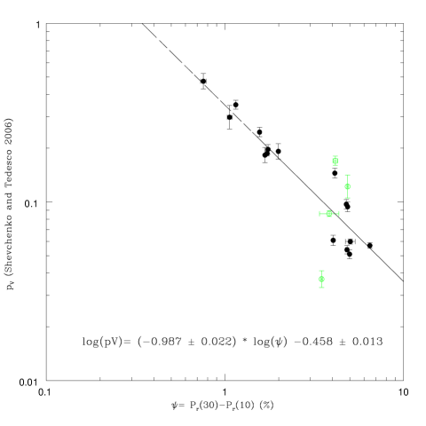
Figure 16: The $\Psi$-albedo relation in log - log scale for $20$ asteroids of the list of Shevchenko and Tedesco (2006) for which we were able to compute the $\Psi$ parameter. Four asteroids having fewer than $10$ polarimetric measurements were not used in the computation of the linear best-fit and are indicated by open, green symbols. The best-fit solution corresponding to the relation $\log(p_{V})=C1\>\log(\Psi)+C_{2}$ is plotted together with the individual data. The best-fit values of the parameters and their nominal uncertainties are also indicated in Table 1.

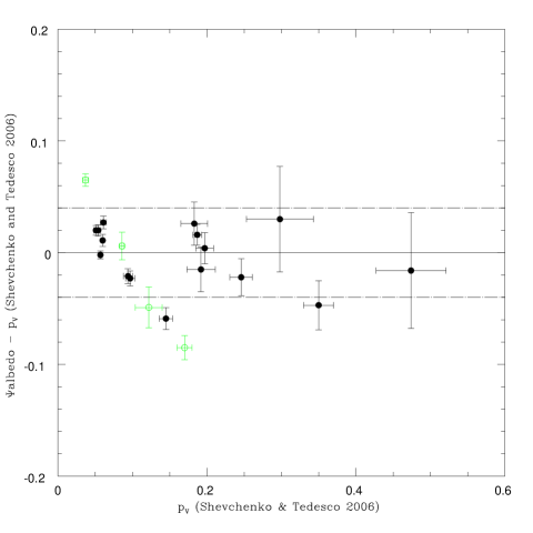
Figure 17: Differences between the albedos of $20$ objects, derived using our calibration of the $\Psi$ - albedo relation, and the corresponding albedo values given by Shevchenko and Tedesco (2006). Four asteroids having fewer than $10$ polarimetric measurements were not used in the computation of the linear best-fit and are indicated by open, green symbols.

The computation of the polarimetric slope from a simple linear fit of data distributed around the inversion angle, or from the computation of the first derivative of $P_{\rm r}$computed at the inversion angle, which would better correspond to the ideal definition of this parameter, is therefore not fully equivalent. It turns out that, opposite to our own expectations, the simpler (purely linear) approach seems to give slightly better results, in spite of all the uncertainties.

The results of the exercises described in this Section are summarized in Table 2, in which we list all the polarimetric parameters considered in our analysis (including some which will be explained in the next Section), and in Table 3, where we list the Shevchenko and Tedesco (2006) values of albedo, together with the corresponding values of albedo derived from the considered polarimetric parameters and their nominal errors. Note that in Table 2, we always give for the inversion angle $\alpha_{\rm inv}$ the value obtained from the best-fit of the whole phase - polarization curve using the exponential - linear relation. Only in cases in which this is not available, but we have at disposal a polarimetric slope $h$ obtained as described in Section 4, we assign to $\alpha_{\rm inv}$ the value corresponding to the intersection of the polarimetric slope with the $P_{\rm r}=0$ line.

The polarimetric parameters $h$, $h_{ABC}$ and $P_{\rm min}$, and corresponding albedos obtained from calibrations based on all and only the objects having albedos larger than $0.08$, as discussed in this and the previous Section, are also listed in Table 5. The improvement of the agreement between the albedos obtained from polarimetric parameters and the albedos given by Shevchenko and Tedesco (2006) is evident. Our considerations about the best possible use of these calibrations have been already exposed in previous Sections.

6 Other polarimetric parameters

The failure of our attempt to obtain more accurate albedo values by using a polarimetric slope ($h_{ABC}$) obtained by a formal computation of the first derivative of Eq. 4 at the inversion angle, can be important. A much simpler linear fit of polarimetric data spread over a large interval of phase angles, seems to be capable of giving slightly more accurate albedo solutions. This can be an indication that using polarimetric parameters describing the behavior of the phase - polarization curve only at some single value of phase angle, or in a limited portion of the phase angle interval, for the determination of the geometric albedo, could be not a very good idea.

Table 2: Summary of the polarimetric parameters found for all asteroids included in the Shevchenko and Tedesco (2006) list, for which we have a suitable coverage of the phase - polarization curves. Each asteroid is identified by its number $N$. The second column gives the number $N_{\rm obs}$ of polarimetric measurements used in the analysis. For the meaning of the other parameters, see the text.

$N$	$N_{\rm obs}$	$h$	$\alpha_{\rm inv}$	$\alpha(P_{\rm min})$	$P_{\rm min}$	$\Psi$	$h_{ABC}$	$p\!\ast$
1	33	0.2549 $\pm$ 0.0041	18.13 $\pm$ 0.02	7.20 $\pm$ 0.02	-1.683 $\pm$ 0.005	4.863 $\pm$ 0.020	0.2467 $\pm$ 0.0009	0.331 $\pm$ 0.015
2	22	0.2223 $\pm$ 0.0015	18.57 $\pm$ 0.02	7.59 $\pm$ 0.07	-1.413 $\pm$ 0.017	4.123 $\pm$ 0.010	0.2111 $\pm$ 0.0004	-0.424 $\pm$ 0.014
3	26	0.1029 $\pm$ 0.0039	20.31 $\pm$ 0.02	8.04 $\pm$ 0.08	-0.732 $\pm$ 0.009	1.724 $\pm$ 0.023	0.0949 $\pm$ 0.0013	-0.863 $\pm$ 0.024
4	26	0.0691 $\pm$ 0.0012	22.37 $\pm$ 0.02	9.22 $\pm$ 0.08	-0.558 $\pm$ 0.005	1.150 $\pm$ 0.006	0.0701 $\pm$ 0.0005	-1.071 $\pm$ 0.025
8	28	0.1067 $\pm$ 0.0016	20.05 $\pm$ 0.02	8.30 $\pm$ 0.03	-0.671 $\pm$ 0.007	1.743 $\pm$ 0.006	0.0950 $\pm$ 0.0003	-0.873 $\pm$ 0.021
27	12	–	21.51 $\pm$ 0.02	7.27 $\pm$ 0.22	-0.593 $\pm$ 0.010	1.062 $\pm$ 0.033	0.0582 $\pm$ 0.0023	–
39	20	0.0745 $\pm$ 0.0093	21.43 $\pm$ 0.02	8.66 $\pm$ 0.07	-0.712 $\pm$ 0.013	1.563 $\pm$ 0.017	0.0906 $\pm$ 0.0009	-0.981 $\pm$ 0.049
41	11	–	22.53 $\pm$ 0.02	10.54 $\pm$ 0.04	-1.664 $\pm$ 0.015	4.040 $\pm$ 0.034	0.2591 $\pm$ 0.0019	–
47	11	–	17.95 $\pm$ 0.02	7.90 $\pm$ 0.20	-1.378 $\pm$ 0.031	5.037 $\pm$ 0.312	0.2412 $\pm$ 0.0109	–
51	20	0.2713 $\pm$ 0.0040	20.35 $\pm$ 0.02	8.29 $\pm$ 0.05	-1.950 $\pm$ 0.015	4.784 $\pm$ 0.023	0.2644 $\pm$ 0.0013	-0.271 $\pm$ 0.015
64	13	0.0434 $\pm$ 0.0043	18.77 $\pm$ 0.02	6.75 $\pm$ 0.26	-0.323 $\pm$ 0.014	0.757 $\pm$ 0.028	0.0395 $\pm$ 0.0014	-1.376 $\pm$ 0.048
78	5	–	22.19 $\pm$ 0.02	10.42 $\pm$ 0.29	-1.497 $\pm$ 0.048	3.835 $\pm$ 0.481	0.2394 $\pm$ 0.0307	–
85	11	0.2648 $\pm$ 0.0071	19.07 $\pm$ 0.02	8.68 $\pm$ 0.16	-1.375 $\pm$ 0.017	4.825 $\pm$ 0.108	0.2414 $\pm$ 0.0034	-0.372 $\pm$ 0.016
105	6	0.2872 $\pm$ 0.0032	19.75 $\pm$ 0.31	–	–	–	–	–
124	5	0.0745 $\pm$ 0.0041	19.79 $\pm$ 1.46	–	–	–	–	–
129	10	0.0953 $\pm$ 0.0077	21.07 $\pm$ 0.02	7.61 $\pm$ 0.03	-0.849 $\pm$ 0.011	1.676 $\pm$ 0.009	0.0928 $\pm$ 0.0004	-0.850 $\pm$ 0.035
216	9	–	18.83 $\pm$ 0.02	8.93 $\pm$ 0.09	-1.028 $\pm$ 0.011	4.151 $\pm$ 0.124	0.1971 $\pm$ 0.0041	–
230	15	0.1045 $\pm$ 0.0047	20.45 $\pm$ 0.02	7.55 $\pm$ 0.06	-0.937 $\pm$ 0.012	1.991 $\pm$ 0.017	0.1089 $\pm$ 0.0010	-0.792 $\pm$ 0.025
324	20	0.2890 $\pm$ 0.0046	19.73 $\pm$ 0.02	8.70 $\pm$ 0.05	-1.655 $\pm$ 0.016	4.987 $\pm$ 0.024	0.2644 $\pm$ 0.0010	-0.292 $\pm$ 0.014
431	7	–	19.67 $\pm$ 0.02	9.29 $\pm$ 0.07	-1.360 $\pm$ 0.024	4.864 $\pm$ 0.048	0.2478 $\pm$ 0.0023	–
444	6	–	20.65 $\pm$ 0.02	9.77 $\pm$ 0.04	-1.098 $\pm$ 0.012	3.477 $\pm$ 0.041	0.1914 $\pm$ 0.0021	–
704	32	0.3074 $\pm$ 0.0054	15.73 $\pm$ 0.02	7.02 $\pm$ 0.01	-1.310 $\pm$ 0.006	6.478 $\pm$ 0.011	0.2692 $\pm$ 0.0006	-0.333 $\pm$ 0.012

Table 3: Resulting albedo values $p_{V}$ for all asteroids belonging to the Shevchenko and Tedesco (2006) list, for which we have polarimetric observations suitable to derive an albedo value using one or more of the techniques explained in the text. Only the albedo corresponding to the calibration computed using all available objects (not only those with $p_{V}>0.08$) are listed. The last column gives, for a comparison, the albedo given by Shevchenko and Tedesco (2006).

Number	$p_{V}(h)$	$p_{V}(h_{ABC})$	$p_{V}(P_{\rm min})$	$p_{V}(\Psi)$	$p_{V}(p\!\ast)$	$p_{V}$(S&T)
1	0.076 $\pm$ 0.006	0.070 $\pm$ 0.004	0.058 $\pm$ 0.001	0.073 $\pm$ 0.003	0.069 $\pm$ 0.004	0.094 $\pm$ 0.006
2	0.088 $\pm$ 0.007	0.083 $\pm$ 0.005	0.074 $\pm$ 0.002	0.086 $\pm$ 0.004	0.084 $\pm$ 0.005	0.145 $\pm$ 0.009
3	0.207 $\pm$ 0.021	0.206 $\pm$ 0.016	0.188 $\pm$ 0.005	0.203 $\pm$ 0.007	0.207 $\pm$ 0.018	0.187 $\pm$ 0.006
4	0.322 $\pm$ 0.033	0.292 $\pm$ 0.025	0.276 $\pm$ 0.008	0.303 $\pm$ 0.009	0.318 $\pm$ 0.031	0.350 $\pm$ 0.020
8	0.199 $\pm$ 0.018	0.206 $\pm$ 0.016	0.213 $\pm$ 0.005	0.201 $\pm$ 0.007	0.212 $\pm$ 0.018	0.197 $\pm$ 0.012
27	–	0.360 $\pm$ 0.036	0.254 $\pm$ 0.008	0.328 $\pm$ 0.014	–	0.298 $\pm$ 0.045
39	0.297 $\pm$ 0.051	0.218 $\pm$ 0.017	0.196 $\pm$ 0.006	0.224 $\pm$ 0.007	0.264 $\pm$ 0.034	0.246 $\pm$ 0.015
41	–	0.066 $\pm$ 0.004	0.059 $\pm$ 0.001	0.088 $\pm$ 0.004	–	0.061 $\pm$ 0.004
47	–	0.071 $\pm$ 0.006	0.077 $\pm$ 0.003	0.071 $\pm$ 0.005	–	0.060 $\pm$ 0.002
51	0.071 $\pm$ 0.005	0.064 $\pm$ 0.004	0.047 $\pm$ 0.001	0.074 $\pm$ 0.003	0.061 $\pm$ 0.003	0.097 $\pm$ 0.006
64	0.540 $\pm$ 0.085	0.560 $\pm$ 0.059	0.600 $\pm$ 0.044	0.458 $\pm$ 0.022	0.597 $\pm$ 0.084	0.474 $\pm$ 0.047
78	–	0.072 $\pm$ 0.011	0.068 $\pm$ 0.003	0.092 $\pm$ 0.012	–	0.086 $\pm$ 0.003
85	0.072 $\pm$ 0.006	0.071 $\pm$ 0.004	0.077 $\pm$ 0.002	0.074 $\pm$ 0.004	0.075 $\pm$ 0.004	0.054 $\pm$ 0.003
105	0.066 $\pm$ 0.005	–	–	–	–	0.047 $\pm$ 0.005
124	0.297 $\pm$ 0.034	–	–	–	–	0.240 $\pm$ 0.036
129	0.226 $\pm$ 0.029	0.212 $\pm$ 0.017	0.152 $\pm$ 0.004	0.209 $\pm$ 0.007	0.202 $\pm$ 0.020	0.183 $\pm$ 0.018
216	–	0.090 $\pm$ 0.006	0.116 $\pm$ 0.002	0.085 $\pm$ 0.004	–	0.170 $\pm$ 0.010
230	0.204 $\pm$ 0.021	0.177 $\pm$ 0.013	0.132 $\pm$ 0.003	0.177 $\pm$ 0.006	0.179 $\pm$ 0.015	0.192 $\pm$ 0.019
324	0.066 $\pm$ 0.005	0.064 $\pm$ 0.004	0.059 $\pm$ 0.002	0.071 $\pm$ 0.003	0.064 $\pm$ 0.003	0.051 $\pm$ 0.003
431	–	0.069 $\pm$ 0.004	0.078 $\pm$ 0.002	0.073 $\pm$ 0.003	–	0.122 $\pm$ 0.018
444	–	0.093 $\pm$ 0.006	0.106 $\pm$ 0.002	0.102 $\pm$ 0.004	–	0.037 $\pm$ 0.004
704	0.061 $\pm$ 0.004	0.063 $\pm$ 0.004	0.082 $\pm$ 0.001	0.055 $\pm$ 0.003	0.069 $\pm$ 0.004	0.057 $\pm$ 0.002

Table 4: Average RMS deviation of polarimetrically-derived albedo with respect to the values in the Shevchenko and Tedesco (2006) list, using different possible albedo - polarization relations described in the text. For each case, $N$ is the number of observed asteroids used to obtain the calibration

Albedo computed from:		RMS deviation	$N$
$h$ slope from linear fit	(all objects)	$0.035$	$15$
$h$ slope from linear fit	(only objects having $p_{V}>0.08$)	$0.033$	$11$
$h_{abc}$ slope from linear-exponential fit	(all objects)	$0.038$	$16$
$h_{abc}$ slope from linear-exponential fit	(only objects having $p_{V}>0.08$)	$0.034$	$11$
$P_{\rm min}$	(all objects)	$0.051$	$16$
$P_{\rm min}$	(only objects having $p_{V}>0.08$)	$0.035$	$11$
$\Psi=P_{\rm r}(30)-P_{\rm r}(10)$	(all objects)	$0.026$	$16$
$p^{*}$	(all objects)	$0.043$	$13$

Table 5: List of polarimetric parameters $h$, $h_{ABC}$ and $P_{\rm min}$ obtained for $15$ asteroids of the Shevchenko and Tedesco (2006) list, having albedo larger than $0.08$, and the corresponding albedos computed using the calibrations based on these objects, only (see Table 1). $N_{tot}$ is the number of polarimetric observations available for each object. The last column gives, for a comparison, the albedo value listed by Shevchenko and Tedesco (2006).

$N$	$N_{\rm tot}$	$h$	$h_{ABC}$	$P_{\rm min}$	$p_{V}(h)$	$p_{V}(h_{ABC})$	$p_{V}(P_{\rm min})$	$p_{V}(ST)$
1	33	$0.2549\pm 0.0041$	$0.2467\pm 0.0009$	$-1.683\pm 0.005$	$0.102\pm 0.010$	$0.101\pm 0.010$	$0.103\pm 0.003$	$0.094\pm 0.006$
2	22	$0.2223\pm 0.0015$	$0.2111\pm 0.0004$	$-1.413\pm 0.017$	$0.114\pm 0.012$	$0.114\pm 0.012$	$0.120\pm 0.003$	$0.145\pm 0.009$
3	26	$0.1029\pm 0.0039$	$0.0949\pm 0.0013$	$-0.732\pm 0.009$	$0.210\pm 0.027$	$0.213\pm 0.026$	$0.213\pm 0.005$	$0.187\pm 0.006$
4	26	$0.0691\pm 0.0012$	$0.0701\pm 0.0005$	$-0.558\pm 0.005$	$0.289\pm 0.040$	$0.270\pm 0.035$	$0.270\pm 0.009$	$0.350\pm 0.020$
8	28	$0.1067\pm 0.0016$	$0.0950\pm 0.0003$	$-0.671\pm 0.007$	$0.204\pm 0.026$	$0.213\pm 0.026$	$0.230\pm 0.006$	$0.197\pm 0.012$
27	12	–	$0.0582\pm 0.0023$	$-0.593\pm 0.010$	–	$0.312\pm 0.043$	$0.256\pm 0.008$	$0.298\pm 0.045$
39	20	$0.0745\pm 0.0093$	$0.0906\pm 0.0009$	$-0.712\pm 0.013$	$0.272\pm 0.046$	$0.221\pm 0.027$	$0.218\pm 0.006$	$0.246\pm 0.015$
51	20	$0.2713\pm 0.0040$	$0.2644\pm 0.0013$	$-1.950\pm 0.015$	$0.097\pm 0.010$	$0.096\pm 0.009$	$0.091\pm 0.003$	$0.097\pm 0.006$
64	13	$0.0434\pm 0.0043$	$0.0395\pm 0.0014$	$-0.323\pm 0.014$	$0.420\pm 0.073$	$0.422\pm 0.063$	$0.434\pm 0.027$	$0.474\pm 0.047$
78	5	–	$0.2394\pm 0.0307$	$-1.497\pm 0.048$	–	$0.104\pm 0.015$	$0.114\pm 0.004$	$0.086\pm 0.003$
124	5	$0.0745\pm 0.0041$	–	–	$0.272\pm 0.039$	–	–	$0.240\pm 0.036$
129	10	$0.0953\pm 0.0077$	$0.0928\pm 0.0004$	$-0.849\pm 0.011$	$0.224\pm 0.032$	$0.217\pm 0.026$	$0.187\pm 0.004$	$0.183\pm 0.018$
216	9	–	$0.1971\pm 0.0041$	$-1.028\pm 0.011$	–	$0.121\pm 0.012$	$0.159\pm 0.003$	$0.170\pm 0.010$
230	15	$0.1045\pm 0.0047$	$0.1089\pm 0.0010$	$-0.937\pm 0.012$	$0.208\pm 0.027$	$0.191\pm 0.022$	$0.172\pm 0.004$	$0.192\pm 0.019$
431	7	–	$0.2478\pm 0.0023$	$-1.360\pm 0.024$	–	$0.101\pm 0.010$	$0.124\pm 0.003$	$0.122\pm 0.018$

According to current evidence, we know that low albedo asteroids exhibit a deeper value of $P_{\rm min}$ as well as a steeper linear polarization slope over a large interval of phase angles. Asteroids having increasingly higher albedos exhibit an opposite behavior (increasingly shallower $P_{\rm min}$ and gentler $h$). There are also differences in the typical values of the inversion angle for different classes of objects, as found, as an example, in the case of the $F$ taxonomic class by Belskaya et al. (2005). One can imagine many different ways to attempt a new calibration of the albedo - polarization relationship trying to exploit the above evidence and make use of the overall morphology of the phase - polarization curve. A first attempt in this direction was proposed by Masiero et al. (2012).

These authors proposed to use a new observable, they called $p\ast$ (p-star), defined as a parameter of maximum polarimetric variation, given by

$$p\ast=W_{1}\log(h)+W_{2}\log(P_{\rm min})$$

where $h$ is, again, the classical polarimetric slope, and $W_{1}$ and $W_{2}$ are two parameters whose values were found by Masiero et al. (2012) to be $W_{1}=0.79\pm 0.02$ and $W_{2}=0.61\pm 0.03$. The authors used in their analysis a data-set of $177$ asteroids having an albedo value estimated from thermal radiometry data produced by the WISE mission, whereas polarimetric data were taken by the authors from the literature. For $65$ asteroids of this sample, the authors derived a value of $h$, while for $112$ objects they derived a value of $P_{\rm min}$. In this way, Masiero et al. (2012) derived a new calibration of the albedo - polarization relationship based on WISE albedos and the newly introduced $p\ast$ parameter. The relation they found was:

$$\log(p_{V})=C\ast_{1}\>p\!\ast+C\ast_{2}$$

and they found for the $C\ast_{1}$ and $C\ast_{2}$ coefficients the values $C\ast_{1}=-1.04\pm 0.04$ and $C\ast_{2}=-1.58\pm 0.09$.

Since we use in our analysis a much smaller number of asteroids having presumably more accurate albedo values not derived from thermal radiometry, and we use a different set of polarimetric data including a large number of previously unpublished observations, we have decided to derive a new calibration of the albedo - $p\ast$ relation, using the data at our disposal, while keeping the same definition of the $p\ast$ parameter as given by Masiero et al. (2012). In particular, we kept the values computed by Masiero et al. (2012) for the $W_{1}$ and $W_{2}$ parameters, which were derived by the authors based on their own analysis of polarimetric data. We computed then the $p\ast$ parameter for our sample of asteroids using $P_{\rm min}$ values already obtained from our best-fit of Eq. 4 and polarimetric slopes $h$ derived as described in Section 4. We had at disposal estimates for both $h$ and $P_{\rm min}$ for $13$ objects, only. The results of this exercise are shown in Fig. 15, in which we also show the new values that we found for the $C\ast_{1}$ and $C\ast_{2}$ parameters. In particular, we have:

$$C\ast_{1}=-0.896\pm 0.029$$

and

$$C\ast_{2}=-1.457\pm 0.018$$

The resulting fit is fairly good, and we confirm that $p\ast$ is another useful parameterfor albedo determination. The resulting RMS deviations, however, are higher than those corresponding to the slope - albedo relation discussed above, both using either $h$ or $h_{abc}$, as shown in Table 4. We find a quite big discrepancy concerning the predicted albedo for (64) Angelina and the corresponding Shevchenko and Tedesco (2006) value. In the region of higher $p\ast$ values (right region of the plot), moreover, the scatter of the albedos around the best-fit line is fairly high.

There are, of course, other possibilities to use polarimetric parameters describing the overall morphology of the observed phase - polarization curves. A very simple idea is to use some parameter built directly from the obtained values of polarization $P_{\rm r}$ taken at very different values of phase angle, possibly including both the negative and the positive polarization branches. In this paper, we introduce such a parameter, that we call $\Psi$, and we define it as

$$\Psi=P_{\rm r}(30^{\circ})-P_{\rm r}(10^{\circ})$$

where the dependence of $P_{\rm r}$ upon the phase angle is assumed to be given by Eq. 4. We derived therefore the $\Psi$ parameter for our sample of asteroids in the Shevchenko and Tedesco (2006) list following the same criteria already described above in the case of our computations of $P_{\rm min}$ and $h_{ABC}$. This corresponds to $20$ asteroids, listed in Table 2. For the purposes of calibration, again, we did not use data of four asteroids having fewer than $10$ polarimetric measurements, which in Fig. 16 are displayed using different symbols. The Figure shows a log - log plot of $\Psi$ as a function of the Shevchenko and Tedesco (2006) albedo, according to the relation

$$\log(p_{V})=C_{\psi 1}\log(\Psi)+C_{\psi 2}$$

identical to the classical slope - albedo relation, but using the new parameter $\Psi$ instead of the polarimetric slope $h$. Fig. 16 shows the best-fit linear solution, and the resulting values of the $C\psi_{1}$ and $C\psi_{2}$ parameters, which are also listed, together with their corresponding uncertainties, in Table 1.

The fit looks good, and this is confirmed by the resulting RMS deviations, which are found to be slightly lower than in the case of all other albedo - polarization relations examined in this paper, including those obtained by excluding low-albedo objects, as shown by the in Table 4. In Fig. 17, we plot the differences between the albedo values produced by our $\Psi$ - albedo calibration and the albedos given by Shevchenko and Tedesco (2006). The albedo values obtained from the $\Psi$ parameter tend to be always very close to the corresponding Shevchenko and Tedesco (2006) values, although the relative uncertainty tends to be fairly high for the darkest asteroids.

With respect to the results obtained by using the polarimetric slope as shown in previous Sections, it is encouraging to note that our $\Psi$ - albedo relation seems to fit nicely the Shevchenko and Tedesco (2006) albedos in the whole interval covered by the data. The albedo obtained for (64) Angelina seems to suggest that we have no longer the problem of a possible overestimation of the albedo of bright objects, which affected the calibration of the classical slope - albedo law, as seen in Section 4. We also note that the value of $C\psi_{1}=-0.987\pm 0.022$, obtained in our calibration of the $\Psi$ - albedo relation, is also formally in agreement, within the uncertainty, with an even simpler hyperbolic relation $p_{V}=K/\Psi$, with $K=10^{C_{2}}\simeq 0.348$.

We find, again, some problems with asteroid (2) Pallas, for which an albedo of $0.086\pm 0.004$ is found by our $\Psi$ calibration, still much lower than the $0.145$ albedo indicated by Shevchenko and Tedesco (2006). The same is true for (216) Kleopatra, which has a $\Psi$ value nearly identical to that of Pallas, corresponding to an albedo of $0.085\pm 0.004$, much lower than the Shevchenko and Tedesco (2006) value of $0.170\pm 0.010$. As opposite, for (444) Gyptis we have problems of a remarkable overestimation of the albedo, but in this case the Shevchenko and Tedesco (2006) albedo is extremely low, $0.037\pm 0.004$. Both Kleopatra and Gyptis are asteroids for which we have fewer than $10$ polarimetric measurements. In the case of (444) Gyptis, the phase - polarization curve is quite noisy, whereas this is not the case for Kleopatra.

7 Conclusions and future work

The solution of the problem of determining the best possible calibration of the relation between geometric albedo and polarization properties for the asteroids is still an important task even in the era of large thermal radiometry surveys, whose results are valid in terms of statistical distribution among large samples of the population, but can be strongly inaccurate for what concerns single objects.

It is therefore very important to optimize the performances of the polarimetric technique, as an effective tool to estimate the albedo of the objects, with particularly important applications to the physical characterization of newly-discovered, and potentially hazardous near-Earth objects. We stress again that, once a reliable calibration of the relation between albedo and polarimetric parameters is available, the albedo values obtained by polarimetric data are not affected at all by uncertainties due to poor knowledge of the absolute magnitude of the objects, a relevant advantage over other possible techniques.

In this paper we have carried out an extensive analysis, based on the idea of using for calibration purposes a still limited number of asteroids for which we can be reasonably confident to know the albedo with good accuracy. We have used this sample to obtain a new calibration of the classical slope - albedo law, with the polarimetric slope being derived from available data using different possible approaches. We have also analyzed other possible relations, including a new calibration of the classical $P_{\rm min}$ - albedo relation, the more recently proposed $p\ast$ - albedo relation (Masiero et al., 2012), and a new relation based on the $\Psi$ polarimetric parameter, introduced for the first time in this paper. The resulting values of the various polarimetric parameters for $22$ asteroids considered in our analysis, and the corresponding values of albedo are given in Tables 2 and 3, respectively.

The extensive analysis presented in this paper produced a variety of interesting results. For what concerns the “classical” slope - albedo and $P_{\rm min}$ - albedo relations, we confirm that it is difficult to find a calibration which can fit accurately objects of all albedo classes. The results improve very much when the asteroids having low albedo, below $0.08$, are not considered in the analysis. The presence of asteroids having significantly different albedo but nearly identical polarimetric slopes can even suggest that a parabolic fit is more suited to represent the $h$ - albedo relation, as shown in Section 4.1 (see Fig. 8).

The calibration of the $h$ albedo and $P_{\rm min}$ - albedo relations that we obtained by excluding low-albedo asteroids from our analysis gives good results, with uncertainties within $\pm 20$% for medium- and high-albedo objects. For asteroids exhibiting a steep polarimetric slope, or having a polarimetric slope computed on the basis of only a few observations, the classical $h$ - albedo relation can still be used, using the calibration coefficients found by considering all the available calibration objects, since the expected errors should be still acceptable. This is encouraging, because whenever there are at least a few measurements obtained at phase angles larger than $14^{\circ}$, it is generally possible to derive a value of the polarimetric slope $h$, and the resulting albedo values turn out to be reasonably accurate in absolute terms, although the relative error can be above $30$% for low-albedo objects. As opposite, the use of $P_{\rm min}$ should always be discouraged for asteroids having a deep negative polarization branch, as seen in Section 5.1.

If one wants to avoid the complication of using different calibrations of the slope - albedo relation for asteroids belonging to different albedo classes, other polarimetric parameters can also be adopted. In particular, both $\Psi$ and $p\ast$ require to have at disposal phase - polarization curves of a sufficiently good quality to be fit by means of an exponential - linear representation (Eq. 4). This cannot be done when the number of polarimetric measurements is too small, or the observations are concentrated over a too limited interval of phase angles. While the uncertainty of albedo determinations based on the $p\ast$ parameter seems to be reasonable but not really negligible, the most accurate albedo determinations can be obtained when the $\Psi$ parameter can be reliably determined from the available data. The advantage of using $\Psi$ is that this parameter seems to be suited to give accurate values of albedo for both bright and dark asteroids.

Of course, there are some caveats to be taken into account. For instance, there are asteroids, like the so-called Barbarians, which exhibit peculiar phase - polarization curves (see Cellino et al., 2006). The determination of the geometric albedo for Barbarian asteroids is a problem, because any derivation of the albedo using relations valid for the rest of the population may be misleading. However, it is also true that more data are needed to better understand the situation.

In fact, the major problem of asteroid polarimetry today is certainly a serious lack of data. Further progress in this field will require the use of dedicated telescopes, to fill the gap with the amount of information already available from other observing techniques.

Polarimetry has been so far severely under-appreciated as an essential tool for physical characterization of asteroids and also other classes of small bodies in the Solar System. The present paper summarizes the current state of the art for what concerns the calibration of the relation between polarimetric properties and albedo, and makes some further steps forward, with the introduction of the $\Psi$ parameter, which seems to be a new useful tool to obtain reliable values of asteroid albedos.

In a separate paper, to be submitted soon for publication, we exploit the results of the present analysis to derive the albedos of a fairly large number of objects for which we lack a Shevchenko and Tedesco (2006) determination, and we analyze the distributions of other parameters that characterize the phase - polarization curves of main belt asteroids.

References

- Bagnulo et al. (1995) Bagnulo, S., Landi Degl’Innocenti, E., Landolfi, M., & Leroy, J.-L. 1995, A&A, 295, 459
- Belskaya et al. (2005) Belskaya, I. N., Shkuratov, Tu., Efimov, Yu., et al. 2005, Icarus, 178, 213
- Bevington (1969) Bevington P.R. 1969, Data reduction and Error analysis for the physical sciences, Mc Graw-Hill Book Company.
- Cañada-Assandri et al. (2012) Cañada-Assandri, M., Gil-Hutton, R. & Benavidez, P. 2012, A&A, 542, A11
- Cellino et al. (1999) Cellino, A., Gil-Hutton, R., Tedesco, E.F., Di Martino, M. & Brunini, A. 1999, Icarus, 138, 129
- Cellino et al. (2006) Cellino, A., Belskaya, I.N., Bendjoya, Ph., Di Martino, M., Gil-Hutton, R., Muinonen, K., & Tedesco, E.F. 2006, Icarus, 180, 565
- Cellino et al. (2012) Cellino, A., Gil-Hutton, R., Dell’Oro, A., Bendjoya, Ph., Cañada-Assandri, M. & Di Martino, M. 2012, JQSRT, 18, 2552
- Cellino et al. (2015) Cellino, A., Ammannito, E., Magni, G., Gil-Hutton, R., Belskaya, I.N., Tedesco, E.F., & De Sanctis, C. 2015, MNRAS (submitted)
- De Leon et al. (2012) De Leon, J., Pinilla-Alonso, N., Campins, H., Licandro, X. & Marzo, G.A. 2012, Icarus, 218, 196
- Gil-Hutton and Cañada-Assandri (2011) Gil-Hutton, R. & Cañada-Assandri, M. 2011, A&A, 529, A86
- Gil-Hutton and Cañada-Assandri (2012) Gil-Hutton, R. & Cañada-Assandri, M. 2012, A&A, 539, A115
- Gil Hutton et al. (2014) Gil Hutton, R., Cellino, A. & Bendjoya, Ph. 2014, A&A, 569, A122
- Kaasalainen et al. (2003) Kaasalainen, S., Piironen, J., Kaasalainen, M., Harris, A.W., Muinonen, K, & Cellino, A. 2003, Icarus, 161, 34
- Lupishko and Mohamed (1996) Lupishko, D.F. & Mohamed, R.A. 1996, Icarus, 119, 209
- Masiero et al. (2011) Masiero, J.R., Mainzer, A.K., Grav., T., et al. 2011, ApJ, 741, 66
- Masiero et al. (2012) Masiero, J.R., Mainzer, A.K., Grav, T., Bauer, J.M., Wright, E.L., Mc Millan, R.S., Tholen, D.J. & Blain, A.W. 2012, ApJ, 749, A104
- Morrison and Lebofsky (1979) Morrison, D. & Lebofsky, L. 1979. In Asteroids (T. Gehrels, Ed.), pp.184-205. Univ. of Arizona Press, Tucson, AZ
- Muinonen et al. (2009) Muinonen, K., Penttila, A., Cellino, A., Belskaya, I. N., Delbo, M., Levasseur-Regourd, A.-C., & Tedesco, E.F. 2009, Meteoritics and Planet. Sci., 44, 1937
- Muinonen et al. (2010) Muinonen, K., Belskaya, I.N., Cellino, A., Delbò, M., Levasseur-Regourd, A.C., Penttila, A. & Tedesco, E.F. 2010, Icarus, 209, 542
- Penttila et al. (2005) Penttila, A., Lumme, K., Hadamcik, E., & Levasseur-Regourd, A.C. 2005, A&A, 432, 1081
- Russel (1916) Russel, H.N. 1916, Ap.J., 43, 173-195