Joint Sparsity Pattern Recovery with 1-bit Compressive Sensing in Sensor Networks

Abstract

We study the problem of jointly sparse support recovery with 1-bit compressive measurements in a sensor network. Sensors are assumed to observe sparse signals having the same but unknown sparse support. Each sensor quantizes its measurement vector element-wise to 1-bit and transmits the quantized observations to a fusion center. We develop a computationally tractable support recovery algorithm which minimizes a cost function defined in terms of the likelihood function and the $l_{1,\infty}$ norm. We observe that even with noisy 1-bit measurements, jointly sparse support can be recovered accurately with multiple sensors each collecting only a small number of measurements.

I Introduction

Support recovery of a sparse signal deals with the problem of finding the locations of the non-zero elements of the sparse signal. This problem occurs in a wide variety of areas including source localization [1, 2], sparse approximation [3], subset selection in linear regression [4, 5], estimation of frequency band locations in cognitive radio networks [6], and signal denoising [7]. In these applications, finding the support of the sparse signal is more important than recovering the complete signal itself. The problem of sparsity pattern recovery has been addressed by many authors in the last decade in different contexts. Compressive sensing (CS) has recently been introduced as a sparse signal acquisition scheme via random projections. A good amount of work has already been done for support recovery with real valued measurements [8, 9, 10, 11]. However, in practice, measurements are quantized before transmission or storage, therefore, it is important to consider quantization of compressive measurements for practical purposes. Further, coarse quantization of measurements is desirable and/or even necessary in resource constrained communication networks. There are some recent works that have addressed the problem of recovering sparse signals/sparsity pattern based on quantized compressive measurements in different contexts, be it calculating performance bounds [12, 13] or devising recovery algorithms [14, 15, 16, 17].

However, most of the work on 1-bit CS has focused only on recovery for the single sensor case. Reliable recovery of a sparse signal based on 1-bit CS is very difficult with only one sensor, especially when the signal-to-noise ratio (SNR) is low. On the other hand, simultaneous recovery of multiple sparse signals arises naturally in a number of applications including distributed sensor and cognitive radio networks. To the best of our knowledge, the problem of jointly sparse support recovery with multiple sensors based on 1-bit CS has not been explored in the literature. In this work, we exploit the benefits of using multiple nodes for jointly sparse recovery with 1-bit CS measurements. We assume that the multiple nodes observe sparse signals with the same but unknown sparsity pattern. The measurement vectors at each node are quantized to 1-bit element-wise and transmitted to a fusion center.

To recover the jointly sparse support, we propose to solve an optimization problem which minimizes an objective function expressed in terms of the likelihood function and the $l_{1,\infty}$ norm of a matrix. We use a computationally tractable algorithm to recover the common sparsity pattern. We show that by employing multiple sensors, the common sparse support can be estimated reliably with a relatively small number of 1-bit CS measurements per node. In particular, we investigate the trade-off between the possibility of deploying multiple sensor nodes and the cost of sampling per node.

II Observation Model

We consider a distributed network with multiple nodes that observe sparse signals having the same sparse support. Let the number of sensors be $P$. At a given node, consider the following $M\times 1$ real valued observation vector collected via random projections:

$$\mathbf{y}_{p}=\boldsymbol{\Phi}_{p}\mathbf{s}_{p}+\mathbf{v}_{p}$$ (1)

where $\boldsymbol{\Phi}_{p}$ is the $M\times N$ ($M<N$) measurement matrix at the $p$-th node for $p=1,\cdots,P$ and $N$ is the signal dimension. For each $p$, the entries of $\boldsymbol{\Phi}_{p}$ are assumed to be drawn from a Gaussian ensemble with mean zero. The sparse signal vector of interest, $\mathbf{s}_{p}$ for $p=1,\cdots,P$, has only $K(\leq N)$ nonzero elements with the same support. The measurement noise vector, $\mathbf{v}_{p}$, at the $p$-th node, is assumed to be independent and identically distributed (i.i.d.) Gaussian with mean vector $\mathbf{0}$ and covariance matrix $\sigma_{v}^{2}\mathbf{I}_{M}$ where $\mathbf{0}$ is a vector of all zeros and $\mathbf{I}_{M}$ is the $M\times M$ identity matrix.

Let each element of $\mathbf{y}_{p}$ be quantized to 1-bit so that the $i$th quantized measurement at the $p$th node is given by,

$$z_{ip}=\left\{\begin{array}[]{ccc}0,{}&~{}\textrm{if}~{}-\infty<y_{ip}<0\\ 1,{}&\textrm{if}~{}0\leq y_{ip}<\infty,\\ \end{array}\right.$$ (4)

where $y_{ip}$ is the $i$th element of $\mathbf{y}_{p}$, for $i=1,2,\cdots,M$ and $p=1,\cdots,P$. Let $\mathbf{Z}$ and $\mathbf{Y}$ be $M\times P$ matrices in which the $(i,p)$-th element of $\mathbf{Z}$ and $\mathbf{Y}$ are $z_{ip}$ and $y_{ip}$ respectively, for $p=1,2,\cdots,P$ and $i=1,\cdots,M$. Further, let $\mathbf{S}$ be the $N\times P$ matrix which contains $\mathbf{s}_{p}$ as its columns for $p=1,2,\cdots,P$. In matrix notation, (4) can be written as,

$$\mathbf{Z}=\mathrm{sign}(\mathbf{Y})$$ (5)

where $\mathrm{sign}(\mathbf{Y})$ denotes the sign of each element of $\mathbf{Z}$.

III Common Support Recovery with 1-bit CS Measurements via $\l_{1}$-Regularized Maximum Likelihood

In this section, first we formulate an optimization problem for joint sparsity pattern recovery for 1-bit CS. We use the regularized $l_{1}$ norm minimization approach with the likelihood function as the cost function instead of the widely used least squares function. With quantized measurements, the approach which uses the likelihood function as the cost function has been shown to provide better results compared to least squares methods with a single sensor [15].

For the sake of tractability, we assume that the measurement matrix $\boldsymbol{\Phi}_{p}=\boldsymbol{\Phi}$ is the same for all $p=1,2,\cdots,P$. We have from (1),

$$y_{ip}=\boldsymbol{\Phi}_{i}^{T}\mathbf{s}_{p}+v_{ip},$$ (6)

for $i=1,2,\cdots,M$ and $p=1,2,\cdots,P$. In the rest of the paper, $\boldsymbol{\Phi}_{i}$ denotes the $i$-th row of $\boldsymbol{\Phi}$.

Next, we calculate probabilities $\Pr(z_{ip}=1)$ and $\Pr(z_{ip}=0)$ which will later be used to write the expression for the likelihood of $\mathbf{Z}$ given S. We have,

$$\Pr(y_{ip}\geq 0)\Rightarrow\Pr(\boldsymbol{\Phi}_{i}^{T}\mathbf{s}_{p}+v_{ip}\geq 0)=\phi(\boldsymbol{\Phi}_{i}^{T}\mathbf{s}_{p}/\sigma_{v}).$$

Similarly,

$$\Pr(y_{ip}<0)\Rightarrow\Pr(\boldsymbol{\Phi}_{i}^{T}\mathbf{s}_{p}+v_{ip}<0)=\phi(-\boldsymbol{\Phi}_{i}^{T}\mathbf{s}_{p}/\sigma_{v}).$$

where $\phi(x)=(1/\sqrt{2\pi})\int_{-\infty}^{x}e^{-t^{2}/2}dt$. The conditional probability of $\mathbf{Z}$ given $\mathbf{S}$ is given by,

$$\Pr(\textbf{Z}|\textbf{S})=\prod_{p=1}^{P}\prod_{i=1}^{M}\Pr(z_{ip}|\textbf{S})$$

$$= \prod_{p=1}^{P}\prod_{i=1}^{M}\left(\phi\left(\frac{\boldsymbol{\Phi}_{i}^{T}\mathbf{s}_{p}}{\sigma_{v}}\right)\right)^{z_{ip}}\times\left(\phi\left(-\frac{\boldsymbol{\Phi}_{i}^{T}\mathbf{s}_{p}}{\sigma_{v}}\right)\right)^{(1-z_{ip})}.$$

The negative log-likelihood of $\mathbf{Z}$ given S, $f_{ml}(\boldsymbol{\Phi}\mathbf{S})$, is given by

$$-\sum_{p=1}^{P}\sum_{i=1}^{M}\left[z_{ip}\log\left(\phi\left(\frac{\boldsymbol{\Phi}_{i}^{T}\mathbf{s}_{p}}{\sigma_{v}}\right)\right)+(1-z_{ip})\log\left(\phi\left(-\frac{\boldsymbol{\Phi}_{i}^{T}\mathbf{s}_{p}}{\sigma_{v}}\right)\right)\right]$$

which can be rewritten as

$$f_{ml}(\textbf{X})=-\sum_{p=1}^{P}\sum_{i=1}^{m}\left[z_{ip}\log\left(\phi\left(\frac{x_{ip}}{\sigma_{v}}\right)\right)\right.\\ +\left.(1-z_{ip})\log\left(\phi\left(\frac{-x_{ip}}{\sigma_{v}}\right)\right)\right],$$ (7)

and $\textbf{X}=\boldsymbol{\Phi}\textbf{S}$. In the following, we use $\mathbf{X}$ and $\Phi\mathbf{S}$ interchangeably. We need to minimize this expression, $f_{ml}(\boldsymbol{\Phi}\mathbf{S})$, as well as incorporate the sparsity condition of the signal matrix $\mathbf{S}$ to obtain an estimated signal matrix $\hat{\mathbf{S}}$ or the support of $\mathbf{S}$. As all the signals observed at all the nodes have the same support, the row-$l_{0}$ norm (as defined in [18] for real valued measurements) is appropriate to incorporate the joint sparsity constraint. The row-$l_{0}$ norm of $\mathbf{S}$ is given by,

$$||\mathbf{S}||_{row-0}=|\textrm{rowsupp}(\mathbf{S})|,$$

which is also referred to as the $l_{0,\infty}$ norm, where the row support of the coefficient matrix $\mathbf{S}$ is defined as [18]

$$\textrm{rowsupp}(\mathbf{S})=\{w\in[1,N]:s_{wk}\neq 0~{}\textrm{for some}~{}k\}.$$

Now to compute $\mathbf{S}$, one can solve the following optimization problem:

$$\underset{\mathbf{S}}{\arg\min}~{}\{f_{ml}(\boldsymbol{\Phi}\textbf{S})+\lambda||\mathbf{S}||_{0,\infty}\}$$ (8)

where $\lambda$ is the penalty parameter. However, the problem (8) is not tractable in its current form and can be relaxed as

$$\underset{{\mathbf{S}}}{\arg\min}~{}\{f_{ml}(\boldsymbol{\Phi}\textbf{S})+\lambda||\mathbf{S}||_{1,\infty}\}$$ (9)

where $||\mathbf{S}||_{1,\infty}=\sum_{i=1}^{N}\underset{1\leq j\leq P}{\max}|s_{ij}|$, i.e., $||\mathbf{S}||_{1,\infty}$ is the sum of all the elements with maximum absolute value in each row, also known as the $l_{1,\infty}$ norm of a matrix.

The goal is to develop a computationally tractable algorithm to solve the problem of the form

$$\underset{\mathbf{S}}{\arg\min}~{}\{f(\boldsymbol{\Phi}\textbf{S})+\lambda g(\mathbf{S})\}$$ (10)

where $f(\boldsymbol{\Phi}\textbf{S})=f_{ml}(\boldsymbol{\Phi}\textbf{S})$ and $g(\mathbf{S})$ is the $l_{1,\infty}$ norm of $\mathbf{S}$.

We use iterative shrinkage-thresholding algorithms (ISTA) for solving the problem defined in (10). In ISTA, each iteration involves solving a simplified optimization problem, which in most of the cases can be easily solved using the proximal gradient method, followed by a shrinkage/soft-threshold step; for e.g., see [19, 20, 21]. From [21], at the $k$-th iteration we have

$${}\mathbf{S}_{k}=P_{L_{f}}(\mathbf{S}_{k-1})$$ (11)

where

$${}P_{L_{f}}(\mathbf{T})=\underset{\hat{\mathbf{S}}}{\operatorname*{arg\,min}}~{}\lambda g(\mathbf{S})+\frac{L_{f}}{2}||\mathbf{S}-(\mathbf{T}-\frac{1}{L_{f}}\nabla f(\mathbf{T})||_{F}^{2}.$$ (12)

Inputs to the algorithm are $L_{f}$ (the Lipshitz constant of $\nabla f$) and $\mathbf{S}_{0}$, the initialization for the iterative method, which can be kept null matrix or $\boldsymbol{\Phi}^{\dagger}\mathbf{Z}$, where $\boldsymbol{\Phi}^{\dagger}$ is the pseudoinverse of $\boldsymbol{\Phi}$ and $\mathbf{Z}$ is the quantized received signal matrix as defined before. For our case, the gradient of $f_{ml}(\mathbf{X})$ w.r.t. matrix S can be easily calculated as $\boldsymbol{\Phi}^{T}\nabla f_{ml}(\textbf{X})$, where $\mathbf{X}=\boldsymbol{\Phi}\textbf{S}$. Notice that, $\nabla f_{ml}(\textbf{X})$ is the gradient of $f_{ml}(\textbf{X})$ w.r.t. X and is given by

$$\nabla f_{ml}(x_{ip})=\frac{z_{ip}\textrm{exp}(-\frac{\tilde{x}_{ip}^{2}}{2})}{\sqrt{2\pi}\sigma_{v}\phi(\tilde{x}_{ip})}-\frac{(1-z_{ip})\textrm{exp}(-\frac{\tilde{x}_{ip}^{2}}{2})}{\sqrt{2\pi}\sigma_{v}\phi(-\tilde{x}_{ip})},$$ (13)

where $\tilde{x}_{ip}=x_{ip}/\sigma_{v}.$

The problem defined in (12) is row separable for each iteration. Therefore, to solve for $\mathbf{S}_{k}$, i.e., to find $P_{L}(\mathbf{S}_{k-1})$, we divide the problem into $N$ subproblems, where $N$ is the number of rows in $\mathbf{S}$. Next, we solve the following subproblem for each row of $\mathbf{S}_{k}$:

$${}\underset{\mathbf{s}^{i}}{\operatorname*{arg\,min}}~{}\lambda g(\mathbf{s}^{i})+\frac{L_{f}}{2}||\mathbf{s}^{i}-(\mathbf{t}^{i}-\frac{1}{L_{f}}\nabla f(\mathbf{t}^{i}))||_{2}^{2};$$ (14)

where $\mathbf{s}^{i}$, $\mathbf{t}^{i}$ and $\nabla f(\mathbf{t}^{i})$ are the $i^{th}$ rows of $\mathbf{S}$, $\mathbf{S}_{k-1}$ and $\nabla f(\mathbf{S}_{k-1})$ respectively. Equation (14) is of the form:

$$\underset{\mathbf{s}}{\arg\min}~{}\left\{\lambda g(\mathbf{s})+\frac{L_{f}}{2}||\mathbf{s}-\mathbf{u}||_{2}^{2}\right\};$$ (15)

where $g(\mathbf{s})=||\mathbf{s}^{i}||_{\infty},$ i.e., the $l_{\infty}$ norm of the $i^{th}$ row of $\mathbf{S}$ and constant vector $\mathbf{u}$ is given by $\mathbf{u}=\mathbf{t}^{i}-\frac{1}{L_{f}}\nabla f(\mathbf{t}^{i})$ (we do not use superscript $i$ on $g(\mathbf{s})$ and $\mathbf{u}$ for brevity).

For (15), we have the following equivalent problem in the epigraph form

$$\underset{\mathbf{s}}{\operatorname*{arg\,min}}~{}\left\{\bar{\lambda}t+\frac{1}{2}||\mathbf{s}-\mathbf{u}||_{2}^{2}\right\},~{}\textrm{s.t.}~{}0\leq\text{sgn}(u_{p})s_{p}\leq t,$$ (16)

where $\bar{\lambda}=\frac{\lambda}{L_{f}}$, $u_{p}$ and $s_{p}$ are the $p$-th elements in $\mathbf{u}$ and $\mathbf{s}$ respectively, for all $p=1,2,\cdots,P$ and $t\in\mathbb{R}$. Define $w_{p}=\text{sgn}(u_{p})$. The problem in (16) can be solved using Lagrangian based methods. The Lagrangian for (16) is

$$L(\mathbf{s},t,\mathbf{\alpha},\mathbf{\beta})=\bar{\lambda}t+\frac{1}{2}\|\mathbf{s}-\mathbf{u}\|_{2}^{2}+\sum_{p}\beta_{p}(w_{p}s_{p}-t)-\sum_{p}\alpha_{p}w_{p}s_{p}$$

with dual variables $\mathbf{\alpha}=[\alpha_{1},\cdots,\alpha_{P}]^{T}$ and $\mathbf{\beta}=[\beta_{1},\cdots,\beta_{P}]^{T}$.

Hence, for strong duality to hold, following Karush–-Kuhn–-Tucker (KKT) conditions must be satisfied by the optimal $\mathbf{s}^{*},t^{*},\mathbf{\alpha}^{*}$ and $\mathbf{\beta}^{*}$.

$$(s_{p}^{*}-u_{p})-\alpha_{p}^{*}w_{p}+\beta_{p}^{*}w_{p}=0,$$ (17)

$$\bar{\lambda}-\sum_{p}\beta_{p}^{*}=0,$$ (18)

$$\alpha_{p}^{*}(w_{p}s_{p}^{*})=0,$$ (19)

$$\beta_{p}^{*}(w_{p}s_{p}^{*}-t^{*})=0,$$ (20)

$$\alpha_{p}^{*},\beta_{p}^{*}\geq 0.$$ (21)

Note that $0\leq w_{p}s_{p}\leq t,\;p=1,\ldots,P$. To find the optimal $\mathbf{s}^{*}$, consider three simple cases

Case (i):

$$w_{p}s_{p}^{*}=0$$

$$\Rightarrow \beta_{p}^{*}=0\;\text{(from (\ref{eq4}))}$$

$$\Rightarrow u_{p}+\alpha_{p}^{*}w_{p}=0\;\text{(from (\ref{eq1}))}$$

$$\Rightarrow \alpha_{p}^{*}=\frac{-u_{p}}{w_{p}}\;\text{which is}\leq 0.$$

Therefore, from (21), $s_{p}^{*}=0$ if and only if $u_{p}=0$.

Case (ii):

$$0<w_{p}s_{p}^{*}<t$$

$$\Rightarrow \beta_{p}^{*}=0\;\text{(from (\ref{eq4})) and}\;\alpha_{p}^{*}=0\;\text{(from (\ref{eq3}))}$$

$$\Rightarrow s_{p}=u_{p}\;\text{(from (\ref{eq1}))}$$

Case (iii):

$$w_{p}s_{p}^{*}=t$$

$$\Rightarrow s_{p}-u_{p}+\beta_{p}^{*}w_{p}=0\;\text{ (from (\ref{eq1}))}$$

$$\Rightarrow \frac{t^{*}}{w_{p}}-u_{p}+\beta_{p}^{*}w_{p}=0$$

$$\Rightarrow \beta_{p}^{*}=\frac{u_{p}}{w_{p}}-\frac{t^{*}}{w_{p}^{2}}$$

$$\Rightarrow \beta_{p}^{*}=|u_{p}|-t^{*}.$$

Also, since $\beta_{p}\geq 0~{}\forall~{}p=[1,2,\cdots,P]$, we have $\beta_{p}^{*}=(|u_{p}|-t^{*})_{+}$, where $(x)_{+}$ is defined as max$(x,0)$.
Using (18) in the above equation, we have

$$\sum_{p}(|u_{p}|-t^{*})_{+}-\bar{\lambda}=0$$ (22)

as $\beta_{p}=(|u_{p}|-t^{*})_{+}$. This can be easily solved for $t^{*}$ by applying the bisection based method using the initial interval $[0,||u||_{\infty}]$. Define

$$g(t)=\sum_{p}(|u_{p}|-t^{*})_{+}-\bar{\lambda}.$$

Therefore, $g(t^{*})=0$. If there exists no solution in the interval $[0,||u||_{\infty}]$, i.e., $g(0)\times g(||u||_{\infty})\geq 0$, the trivial solution is given by $t^{*}=0.$ Once we have the optimal $t^{*}$, the optimal $s^{*}$ is given by

$$s_{p}^{*}=\left\{\begin{array}[]{c}w_{p}t^{*}~{}\textrm{if}~{}|u_{p}|\geq t^{*};\\ u_{p}~{}\textrm{otherwise}.\\ \end{array}\right.$$ (23)

Each subproblem given by (14) can be solved in a similar way, the solution to each of which can be used to find $\mathbf{S}_{k}$ using (11) and (12). The summary of all the steps is provided in Algorithm 1 where $||.||_{F}$ denotes the Frobenius norm. Algorithm 1 produces the matrix $\mathbf{S}_{k}$ and locations of non-zero elements in $\mathbf{S}_{k}$ gives the support of original signal matrix $\mathbf{S}$.

1. Given tolerance $\epsilon{>}0$, parameters $\tilde{\lambda}{>}\lambda,~{}0{<}\alpha{<}1~{}\textrm{and}~{}L_{f}$

2. Initialize $\mathbf{S}_{0}$ ($\mathbf{S}_{-1}=\mathbf{S}_{0}$), $~{}\hat{\lambda}=\tilde{\lambda}$, $k=0$

3. While $~{}\hat{\lambda}>\lambda$

4. $\hat{\lambda}=\alpha\hat{\lambda}$

5. While $||\mathbf{S}_{k}-\mathbf{S}_{k-1}||_{F}>\epsilon||\mathbf{S}_{k-1}||_{F}$

6. $k=k+1$

7. Define matrix $\mathbf{U}=\mathbf{S}_{k-1}-\frac{1}{L_{f}}\nabla f(\mathbf{S}_{k-1})$ where $\nabla f(\mathbf{S}_{k-1})$ is computed as in (13)

8. For each row of $\mathbf{S}_{k}$

9. Update the $p$-th row element using (23) for $p=1,2,\cdots,P$

10. End For

11. End While

12. End While

Algorithm 1 Estimation of the common support of the sparse signal

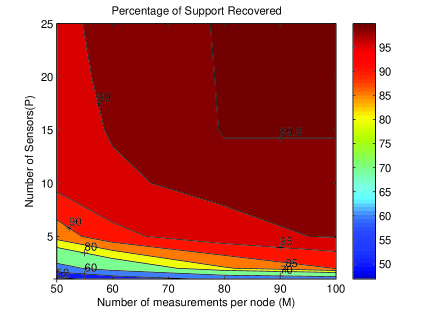
(a) Percentage of Support Recovered

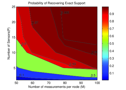
(b) Probability of Recovering Exact Support

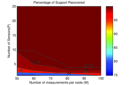
Figure 1: Performance of common sparsity pattern recovery when $\sigma_{v}^{2}=0.01$

(a) Percentage of Support Recovered

(b) Probability of Recovering Exact Support

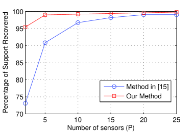
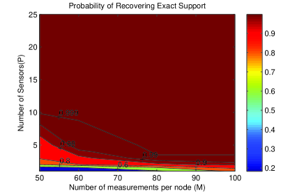
Figure 2: Performance of common sparsity pattern recovery when $\sigma_{v}^{2}=0.0001$

(a) Percentage Support Recovery

(b) Probability of Estimating Exact Support

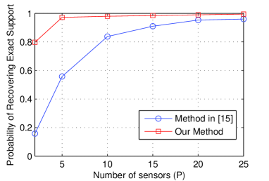
Figure 3: Comparison of our results with the approach presented in [15]: $M=50$, $N=100$ and $K=5$, in terms of the percentage of support recovered correctly and the probability of recovering exact support

IV Numerical Results

In this section, we present some simulation results to demonstrate the performance of jointly sparse support recovery with 1-bit CS based on our proposed algorithm. For every Monte Carlo run, we generate the elements of the $M\times N$ measurement matrix $\boldsymbol{\Phi}$ from a normal distribution with mean zero and variance = 0.004. In all our simulations, we used randomly generated sparse signal matrix $\mathbf{S}$, with each column size fixed as $N=100$. We choose $K$ random values out of $N$, which are the nonzero rows in $\mathbf{S}$. For each column of $\mathbf{S}$, all the elements whose position is given by the $K$ random values are assigned a value of either $1$ or $-1$ with probability $0.5$. The value of $K$ is kept $5$. The observation noise is assumed to be Gaussian with mean zero and variance is $\sigma_{v}^{2}=0.01$ (SNR = 2.96 dB, low SNR case), and $\sigma_{v}^{2}=0.0001$ (SNR = 23.01 dB, high SNR case). We measure the percentage of support recovered correctly and the probability of recovering exact support as $M$, $P$ and SNR vary using $1000$ Monte Carlo runs.

Our results for low SNR regime are plotted in Fig. 1. The y-axis shows the number of sensors ($P$) and the x-axis shows the number of measurements per node ($M$). In Fig. 1 (a), the numbers on contours represent the percentage of support that are recovered. Similarly, in Fig. 1(b), the numbers on contours represent the probability of recovering the exact support. We can deduce that for a particular value of $M$, the performance improves with the number of sensors, and vice-versa. Similarly, Fig. 2 shows the contour plots in the high SNR regime. We see that even with a very small number of sensors, for e.g., $P=3$, the algorithm performs very well for reasonable values for $M$, such as $M=60$.

In Fig. 3, we compare our results with one of the most related algorithms for sparse recovery with quantized measurements as provided in [15], which uses the ML method for only one node (one measurement vector). To compute the common support with $P$ measurement vectors, the individual support sets were computed for each signal using the algorithm in [15], and the estimated support sets were fused using the majority rule. For comparison, values of $M$, $N$ and $K$ were chosen as 50, 100 and 5, respectively. The observation noise variance $\sigma_{v}^{2}=0.0001$. As seen from Fig. 3, our proposed approach for joint sparsity pattern recovery with quantized measurements outperforms the case when the support is estimated individually as in [15] and then fused. In particular, the proposed algorithm in this paper exploits the jointly sparse nature of multiple measurement vectors thus outperforming the results obtained by estimating the supports individually using [15] and then fused.

V Conclusion

In this paper, we exploited the use of multiple sensors for the recovery of common sparsity pattern of sparse signals with 1-bit CS. A computationally tractable algorithm was developed to optimize an objective function defined in terms of likelihood function and the $l_{1,\infty}$ norm of a matrix. Numerical results show that, with very coarsely quantized measurements (only the sign information), the common sparsity pattern of sparse signals can be recovered reliably even in the low SNR region, and the performance increases monotonically with the number of sensors.

References

• [1] D.ย Malioutov, M.ย Cetin, and A.Willsky, โ€œA Sparse Signal Reconstruction Perspective for Source Localization with Sensor Arrays,โ€ IEEE Trans. Signal Processing, vol.ย 53, no.ย 8, pp. 3010โ€“3022, Aug. 2005.
• [2] V.ย Cevher, P.ย Indyk, C.ย Hegde, and R.ย G. Baraniuk, โ€œRecovery of Clustered Sparse Signals from Compressive Measurements,โ€ in Int. Conf. Sampling Theory and Applications (SAMPTA 2009), Marseille, France, May. 2009, pp. 18โ€“22.
• [3] B.ย K. Natarajan, โ€œSparse Approximate Solutions to Linear Systems,โ€ SIAM J. Computing, vol.ย 24, no.ย 2, pp. 227โ€“234, 1995.
• [4] A.ย J. Miller, Subset Selection in Regression.ย ย ย New York, NY: Chapman-Hall, 1990.
• [5] E.ย G. Larsson and Y.ย Selen, โ€œLinear Regression With a Sparse Parameter Vector,โ€ IEEE Trans. Signal Processing, vol.ย 55, no.ย 2, pp. 451โ€“460, Feb.. 2007.
• [6] Z.ย Tian and G.ย Giannakis, โ€œCompressed Sensing for Wideband Cognitive Radios,โ€ in Proc. Acoust., Speech, Signal Processing (ICASSP), Honolulu, HI, Apr. 2007, pp. IVโ€“1357โ€“IVโ€“1360.
• [7] S.ย S. Chen, D.ย L. Donoho, and M.ย A. Saunders, โ€œAtomic Decomposition by Basis Pursuit,โ€ SIAM J. Sci. Computing, vol.ย 20, no.ย 1, pp. 33โ€“61, 1998.
• [8] M.ย J. Wainwright, โ€œInformation-theoretic limits on sparsity recovery in the high-dimensional and noisy setting,โ€ IEEE Trans. Inform. Theory, vol.ย 55, no.ย 12, pp. 5728โ€“5741, Dec. 2009.
• [9] A.ย K. Fletcher, S.ย Rangan, and V.ย K. Goyal, โ€œNecessary and sufficient conditions for sparsity pattern recovery,โ€ IEEE Trans. Inform. Theory, vol.ย 55, no.ย 12, pp. 5758โ€“5772, Dec. 2009.
• [10] M.ย M.ย Akcakaya and V.ย Tarokh, โ€œShannon-theoretic limits on noisy compressive sampling,โ€ IEEE Trans. Inform. Theory, vol.ย 56, no.ย 1, pp. 492โ€“504, Jan. 2010.
• [11] G.ย Tang and A.ย Nehorai, โ€œPerformance analysis for sparse support recovery,โ€ IEEE Trans. Inform. Theory, vol.ย 56, no.ย 3, pp. 1383โ€“1399, March 2010.
• [12] T.ย Wimalajeewa and P.ย Varshney, โ€œPerformance Bounds for Sparsity Pattern Recovery With Quantized Noisy Random Projections,โ€ Selected Topics in Signal Processing, IEEE Journal of, vol.ย 6, no.ย 1, pp. 43โ€“57, Feb 2012.
• [13] G.ย Reeves and M.ย Gastpar, โ€œA Note on Optimal Support Recovery in Compressed Sensing,โ€ in Signals, Systems and Computers, 2009 Conference Record of the Forty-Third Asilomar Conference on, Nov 2009, pp. 1576โ€“1580.
• [14] H.ย Wang and Q.ย Wan, โ€œOne Bit Support Recovery,โ€ in Wireless Communications Networking and Mobile Computing (WiCOM), 2010 6th International Conference on, Sept 2010, pp. 1โ€“4.
• [15] A.ย Zymnis, S.ย Boyd, and E.ย Candes, โ€œCompressed Sensing With Quantized Measurements,โ€ Signal Processing Letters, IEEE, vol.ย 17, no.ย 2, pp. 149โ€“152, Feb 2010.
• [16] Y.ย Plan and R.ย Vershynin, โ€œOne-Bit Compressed Sensing by Linear Programming,โ€ Communications on Pure and Applied Mathematics, vol.ย 66, no.ย 8, pp. 1275โ€“1297, 2013. [Online]. Available: http://dx.doi.org/10.1002/cpa.21442
• [17] P.ย Boufounos and R.ย Baraniuk, โ€œ1-Bit compressive sensing,โ€ in Information Sciences and Systems, 2008. CISS 2008. 42nd Annual Conference on, March 2008, pp. 16โ€“21.
• [18] J.ย A. Tropp, โ€œAlgorithms for simultaneous sparse approximation. Part II: Convex relaxation ,โ€ EURASIP Journal of Signal Processing, vol.ย 86, no.ย 3, pp. 589 โ€“ 602, 2006.
• [19] I.ย Daubechies, M.ย Defrise, and C.ย Deย Mol, โ€œAn Iterative Thresholding Algorithm for Linear Inverse Problems with a Sparsity Constraint,โ€ Communications on Pure and Applied Mathematics, vol.ย 57, no.ย 11, pp. 1413โ€“1457, 2004. [Online]. Available: http://dx.doi.org/10.1002/cpa.20042
• [20] S.ย Wright, R.ย Nowak, and M.ย Figueiredo, โ€œSparse Reconstruction by Separable Approximation,โ€ Signal Processing, IEEE Transactions on, vol.ย 57, no.ย 7, pp. 2479โ€“2493, July 2009.
• [21] A.ย Beck and M.ย Teboulle, โ€œA Fast Iterative Shrinkage-Thresholding Algorithm for Linear Inverse Problems,โ€ SIAM Journal on Imaging Sciences, vol.ย 2, no.ย 1, pp. 183โ€“202, 2009. [Online]. Available: http://dx.doi.org/10.1137/080716542