Optimization algorithms for the solution of the frictionless normal contact between rough surfaces

Abstract

This paper revisits the fundamental equations for the solution of the frictionless unilateral normal contact problem between a rough rigid surface and a linear elastic half-plane using the boundary element method (BEM). After recasting the resulting Linear Complementarity Problem (LCP) as a convex quadratic program (QP) with nonnegative constraints, different optimization algorithms are compared for its solution: ($i$) a Greedy method, based on different solvers for the unconstrained linear system (Conjugate Gradient CG, Gauss-Seidel, Cholesky factorization), ($ii$) a constrained CG algorithm, ($iii$) the Alternating Direction Method of Multipliers (ADMM), and ($iv$) the Non-Negative Least Squares (NNLS) algorithm, possibly warm-started by accelerated gradient projection steps or taking advantage of a loading history. The latter method is two orders of magnitude faster than the Greedy CG method and one order of magnitude faster than the constrained CG algorithm. Finally, we propose another type of warm start based on a refined criterion for the identification of the initial trial contact domain that can be used in conjunction with all the previous optimization algorithms. This method, called Cascade Multi-Resolution (CMR), takes advantage of physical considerations regarding the scaling of the contact predictions by changing the surface resolution. The method is very efficient and accurate when applied to real or numerically generated rough surfaces, provided that their power spectral density function is of power-law type, as in case of self-similar fractal surfaces.

and

1 Introduction

Contact mechanics between rough surfaces is a very active area of research for its paramount importance to address several practical applications in physics and engineering. Understanding the evolution of the contact domain and contact variables, such as load, real contact area, contact stiffness, and many others, that depend on the morphological properties of roughness, is still considered a challenging problem today. The reader is referred to (Barber, 2003; Nosonovsky and Bhushan, 2005; Ciavarella et al., 2006; Hyun and Robbins, 2007; Ciavarella et al., 2008a, b; Carbone and Bottiglione, 2008; Paggi and Ciavarella, 2010; Campaña et al., 2011; Paggi and Barber, 2011; Paggi et al., 2014; Yastrebov, 2014) for an overview of research results developed during the last decade.

Semi-analytical contact theories that are able to provide synthetic predictions of the contact response is also a challenging topic. A comparison and validation on benchmark results is necessary to understand the limitations of existing approaches and propose further improvements. Experimental investigations are difficult to make and involve approximations, for example very often the contact parameters can only be estimated by indirect measurements of thermal or electric resistances of compressed rough joints (McCool, 1986; Sridhar and Yovanovich, 1994) or are mostly limited to measurements of real contact area under special conditions (O’Callaghan and Probert, 2005; Hendriks and Visscher, 1995). Therefore, numerical methods are essential to acquire as much information as possible about the contact problem at hand and infer general conclusions.

In spite of its effectiveness and versatility, the finite element method (FEM) has been mainly applied in mechanics to solve contact problems between rough surfaces in which the constitutive behavior of the bulk is not linear elastic. For instance, the study of elasto-plastic contact problems with roughness (Hyun et al., 2004), where an explicit approach was used to reduce the high computational cost, and the study involving frictional dissipative phenomena in visco-elastic materials, where the energy dissipation in the bulk is essential and can be well predicted by FEM (Wriggers and Reinelt, 2009), are worth mentioning.

In the linear elastic regime, when the multi-scale character of roughness covering a wide spectrum of wavelengths is the main focus, the use of the boundary element method (BEM) is historically preferred over FEM (Andersson, 1981; Man, 1994). This is essentially due to the fact that only the surface must be discretized and not the bulk. Moreover, it is not necessary to adopt surface interpolation techniques, like Bezier curves, to discretize the interface (see, e.g., the rigorous studies in (Wriggers, 2006, Ch. 9) and (Hyun et al., 2004)), which must be used with care to avoid smoothing out artificially the fine scale geometrical features of roughness.

In the application of BEM, the frictionless contact problem between two linear elastic rough surfaces is mathematically equivalent to the problem of the normal contact between a rigid rough surface and an elastic half-plane with equivalent elastic parameters, see (Barber, 2003) for a rigorous proof. The core of BEM is based on the so-called Green’s functions, that relate the displacement of a generic point of the half-plane to the action of a concentrated force on the surface caused by contact interactions. An integral convolution of all the contact tractions provides the deformed contact configuration. After introducing a discretization of the half-plane consisting of a grid of boundary elements, the problem of point-force singularity is solved numerically by using the closed-form solution for a patch load acting on a finite-size boundary element (Johnson, 1985, Ch. 3,4). The contact problem is then set in terms of equalities and inequalities stemming from the unilateral contact constraints and can be solved by constrained optimization. In this regard, apart from the discretization error intrinsic in any numerical method, BEM provides the highest attainable accuracy for discrete problems (Polonsky and Keer, 1999). The basic version of BEM can be also extended to solve rough contact problems with friction (Li and Berger, 2003; Pohrt and Li, 2014) and between viscoelastic materials (Carbone and Putignano, 2013).

With the aim of investigating the effect of roughness at multiple scales, the availability of computational methods that can solve large contact problems in an efficient and fast way is of crucial importance. The size of the linear system of equations relating the contact pressures to the normal deflections can be in fact quite large, as it arises from high resolution profilometric surface samples of 512$\times$512 heights and very large indentations. Hence, the computational challenges regard two main aspects: $(i)$ efficiently solve the system of linear equations; $(ii)$ impose the satisfaction of the unilateral contact constraints (contact inequalities). Regarding the first issue, iterative methods like the Conjugate Gradient algorithm or the Gauss-Seidel method (Francis, 1983; Borri-Brunetto et al., 1999, 2001) have been widely used. Alternatively, the capabilities of multigrid or multilevel methods have been exploited (Raous, 1999; Polonsky and Keer, 1999) to approximately solve the equation system on coarse grids and then project the results on finer grids. Finally, we mention the fast method and its variants based on the solution of the linear system of equations in the Fourier space (see, e.g., (Nogi and Kato, 1997; Polonsky and Keer, 2000a, b; Batrouni et al., 2002; Scaraggi et al., 2013; Prodanov et al., 2014)).

Regarding the imposition of the contact inequalities, (Johnson, 1985, p.149-150) suggested to apply a greedy approach: after solving the equation set for the unknown tractions, the boundary elements for which these are negative (tensile) are excluded in a following iteration from the assumed contact area and the corresponding pressures set equal to zero. Johnson (1985)[p.149-150] stated that “experience confirms that repeated iterations converge to a set of values of pressures which are positive where contact takes place and zero otherwise”. To the best of the authors’ knowledge, a rigorous proof of convergence of this method has not been found in the literature. However, if valid, it allows to use any numerical method to solve the unconstrained set of linear equations and then impose a correction in a recursive way. Indeed, this numerical approach has been successfully applied by many authors, such as Kubo et al. (1981) and Borri-Brunetto et al. (1999, 2001) who used this greedy approach in conjunction with a Gauss-Seidel iterative algorithm for the solution of the unconstrained set of linear equations, and Karpenko and Akay (2001) and Batrouni et al. (2002) who applied it together with a numerical scheme based on the Fast Fourier Transform (FFT).

In alternative to the greedy approach, Polonsky and Keer (1999) proposed a constrained Conjugate Gradient method based on the theory in (Hestenes, 1980, Ch. 2,3) to solve the linear system of equations and rigorously impose the satisfaction of the contact constraints. For the solution of the system of equations, a multi-grid solution scheme was proposed in (Polonsky and Keer, 1999) and then a FFT algorithm was considered in (Polonsky and Keer, 2000a, b).

In this paper, we first examine the validity of the greedy approach based on a monotonic elimination of tensile points. We show that this approach usually finds the exact solution but, as we prove by a counter-example, it may fail. Then, we show that other optimization algorithms such as Non-Negative Least Squares (NNLS) and the Alternative Direction Method of Multipliers (ADMM) can be used in alternative to the greedy approach, by exploiting the equivalence between the contact problem and quadratic programming with unilateral non-negativity constraints. Moreover, we propose warm starting techniques for the optimization algorithms that are especially useful in case of a solution of a sequence of increasing or decreasing displacements.

This paper provides a comprehensive comparison of the computational performance of the greedy approach (used in conjunction with different unconstrained solvers like the Conjugate Gradient, the Gauss-Seidel iterative scheme, or the MATLAB’s mldivide solver), of the original constrained CG method by (Polonsky and Keer, 1999), and of novel optimization algorithms that are able to exploit warm starts for solving convex quadratic programs subject to non-negativity constraints. As a main conclusion, the proposed NNLS algorithm with warm start based on accelerated gradient projections (GPs) is found to be one order of magnitude faster than the algorithm by Polonsky and Keer (1999) and two orders of magnitude faster than the greedy approach.

Finally, by exploiting the morphological features of the contact domain of fractal surfaces, we propose in this paper a cascade multi-resolution algorithm that can further reduce computation time by at least a factor two with respect to the NNLS algorithm with accelerated GPs.

2 Mathematical formulation

In the framework of BEM, the normal displacements $u(\mathbf{x})$ at any point of the half-plane identified by the position vector $\mathbf{x}$ are related to the contact pressures $p(\mathbf{y})$ at other points as follows (Johnson, 1985; Barber, 2010):

$$u(\mathbf{x})=\int_{S}H(\mathbf{x},\mathbf{y})p(\mathbf{y})\mbox{d}\mathbf{y},$$ (1)

where $H(\mathbf{x},\mathbf{y})$ represents the displacement at a point $\mathbf{x}$ due to a surface contact pressure $p$ acting at $\mathbf{y}$ and $S$ is the elastic half-plane. For homogeneous, isotropic, linear elastic materials, the influence coefficients are:

$$H(\mathbf{x},\mathbf{y})=\dfrac{1-\nu^{2}}{\pi E}\dfrac{1}{\parallel\mathbf{x}-\mathbf{y}\parallel},$$ (2)

where $E$ and $\nu$ denote, respectively, the composite Young’s modulus and Poisson’s ratio of half-plane, and $\|\cdot\|$ the standard Euclidean norm. The total contact force $P$ is the integral of the contact pressure field

$$P=\int_{S}p(\mathbf{x})\mbox{d}\mathbf{x}.$$ (3)

By referring to Fig. 1, in the following we define for each surface point $\mathbf{x}\in S$ its elevation $\xi(\mathbf{x})$, measured with respect to a reference frame, and set $\xi_{\rm max}\triangleq\max_{\mathbf{x}\in S}\xi(\mathbf{x})$ the maximum elevation. The indentation of the half plane at the points in contact is denoted by $\bar{u}$, whereas a generic displacement along the surface is $u$.

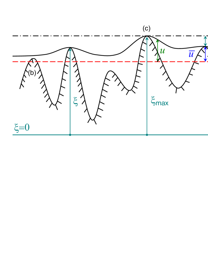
Figure 1: Sketch of the contact problem between a rigid rough surface and an elastic half-plane. Its deformed configuration corresponding to the imposed far-field displacement $\Delta$ is depicted with a black solid line. The red dashed line corresponding to a rigid-body motion of the half-plane identifies the heights to be included in the initial trial contact domain. Once Problem 1 is solved we may have: ($i$) heights certainly not in contact from the beginning, type $(a)$; ($ii$) heights loosing contact due to elastic interactions, type (b); ($iii$) heights in contact, type (c).

We consider the following problem:

Problem 1

For a given far-field displacement $\Delta\geq 0$ in the direction perpendicular to the undeformed half-plane, find the solution of the normal contact problem $u(\mathbf{x})$, $p(\mathbf{x})$ satisfying (1) and the unilateral contact (linear complementarity) conditions

$$u(\mathbf{x})-\bar{u}(\mathbf{x},\Delta) \geq 0,$$ (4a)

$$p(\mathbf{x}) \geq 0,$$ (4b)

$$(u(\mathbf{x})-\bar{u}(\mathbf{x},\Delta))p(\mathbf{x}) =0,$$ (4c)

for all points $\mathbf{x}\in S$, where contact tractions are positive when compressive.

Introducing the quantity $w(\mathbf{x},\Delta)=u(\mathbf{x})-\bar{u}(\mathbf{x},\Delta)$, Eq.(4) can be rewritten as:

$$w(\mathbf{x},\Delta) \geq 0,$$ (5a)

$$p(\mathbf{x}) \geq 0,$$ (5b)

$$w(\mathbf{x},\Delta)p(\mathbf{x}) =0.$$ (5c)

Problem 1 is an infinite-dimensional linear complementarity problem. We find a finite-dimensional approximate solution by discretizing the surface as a square grid of spacing $\delta$ consisting of $N\times N$ average heights. Let $S_{ij}$ be the cell of area $\delta^{2}$ indexed by $i,j\in I_{N}$, with $I_{N}\triangleq\{1,...,N\}\times\{1,...,N\}$. Let $\mathbf{x}_{i,j}\triangleq\int_{\mathbf{x}\in S_{ij}}\mathbf{x}\textrm{d}\mathbf{x}$, $\xi_{i,j}\triangleq\int_{\mathbf{x}\in S_{ij}}\xi(\mathbf{x})\textrm{d}\mathbf{x}$, $p_{i,j}\triangleq\int_{\mathbf{x}\in S_{ij}}p(\mathbf{x})\textrm{d}\mathbf{x}$, and $u_{i,j}\triangleq\int_{\mathbf{x}\in S_{ij}}u(\mathbf{x})\textrm{d}\mathbf{x}$ be, respectively, the barycentric coordinate, average height, resultant of the contact pressures, and the corresponding displacement on the surface element $S_{ij}$. Consider the following discretized version of (1)

$$u_{i,j}=\sum_{k=1}^{N}\sum_{l=1}^{N}H_{i-k,j-l}\,p_{k,l}$$ (6)

for all $(i,j)\in I_{N}$, where the term $H_{i-k,j-l}$ is the Green function used in (1) averaged over the elementary area $\delta^{2}$, which corresponds to the displacement induced by a uniformly loaded square:

$$H_{i-k,j-l}=\dfrac{1}{\delta^{2}}\int_{S_{ij}}\int_{S_{kl}}H(\mathbf{x},\mathbf{y})\text{d}\mathbf{y}\text{d}\mathbf{x},$$ (7)

and

$$p_{k,l}\geq 0,\ \forall(k,l)\in I_{N}.$$ (8)

For instance, Borri-Brunetto et al. (1999) used the following approximation related to a uniform pressure acting on a rounded patch of radius $\delta/2$:

$$H_{i-k,j-l}=\left\{\begin{array}[]{ll}\dfrac{2}{E\pi\delta},&\hbox{if $i=k$ and $j=l$}\\ \dfrac{2}{E\pi\delta}\arcsin\dfrac{\delta}{2\|\mathbf{x}_{i,j}-\mathbf{x}_{k,l}\|},&\hbox{if $i\neq k$, $j\neq l$}\end{array}\right.$$ (9)

but other formulae for a square patch can also be taken as in (Pohrt and Li, 2014).

Let $\bar{I}_{C}\triangleq\{(i,j)\in I_{N}:\ \xi_{i,j}<\xi_{\rm max}-\Delta\}$ be the set of indices corresponding to elements $S_{ij}$ that are certainly not in contact (cf. Fig. 1), and hence

$$p_{k,l}=0,\forall(k,l)\in\bar{I}_{C},$$ (10)

let $m=\#\bar{I}_{C}$ be the number of elements of $\bar{I}_{C}$ and $n=\#I_{C}$ the number of elements belonging to the initial trial contact domain, $I_{C}\triangleq I_{N}\setminus\bar{I}_{C}$. The set $I_{C}$ is only a superset of the set $I_{C}^{*}$ of actual contact points, since the corrections to the displacements induced by elastic interactions may induce lack of contact in some elements $(i,j)$, i.e., $u_{i,j}>\bar{u}_{i,j}$, where $\bar{u}_{i,j}\triangleq\Delta-\xi_{\rm max}+\xi_{i,j}$ is the value of the compenetration of the height corresponding to the element $(i,j)$ in the half-plane (see Fig. 1).

For a generic $(i,j)\in I_{C}$ corresponding to an element of the surface which is potentially in contact with the elastic half-plane, we denote by

$$w_{i,j}\triangleq u_{i,j}-\bar{u}_{i,j}\geq 0$$ (11)

the corresponding elastic correction to the displacement. Clearly, it must hold that

$$w_{i,j}p_{i,j}=0,\ \forall(i,j)\in I_{C}$$ (12)

since $w_{i,j}>0$ implies no contact between the surfaces and therefore no pressure, while $p_{i,j}>0$ implies contact, $u_{i,j}=\bar{u}_{i,j}$, or equivalently $w_{i,j}=0$.

By taking into account that $p_{k,l}=0$ for all $(k,l)\in\bar{I}_{C}$, Eq. (6) can be recast as the following condition

$$w_{i,j}+\bar{u}_{i,j}=\sum_{(k,l)\in I_{C}}H_{i-k,j-l}\,p_{k,l},\ \forall(i,j)\in I_{C},$$ (13)

which is limited to the nodes belonging to the initial trial contact domain $I_{C}$, whose number of elements is in general significantly smaller than those of $I_{N}$. The relations (8)-(13) can be recast in matrix form as the following Linear Complementarity Problem (LCP) (Cottle et al., 1992):

$$\mathbf{w}=\mathbf{H}\mathbf{p}-\bar{\mathbf{u}}$$ (14a)

$$\mathbf{w}\geq\mathbf{0},\ \mathbf{p}\geq\mathbf{0},\ \mathbf{w}^{\prime}\mathbf{p}=0,$$ (14b)

where $\mathbf{w}\in\mathbb{R}^{n}$ is the vector of unknown elastic corrections $w_{i,j}$, $(i,j)\in\bar{I}_{C}$, $\mathbf{w}^{\prime}$ denotes its transpose, $\mathbf{p}\in\mathbb{R}^{n}$ is the vector of unknown average contact forces $p_{i,j}$, $(i,j)\in I_{C}$, $\bar{\mathbf{u}}\in\mathbb{R}^{n}$ is the vector of compenetrations $\bar{u}_{i,j}$, $(i,j)\in I_{C}$, and $\mathbf{H}=\mathbf{H}^{\prime}$ is the matrix obtained by collecting the compliance coefficients $H_{i-k,j-l}$, for $(i,j),(k,l)\in I_{C}$. Due to the properties of linear elasticity (Johnson, 1985, p.144) we have that

$$\mathbf{H}=\mathbf{H}^{\prime}\succ 0,$$ (15)

that is $\mathbf{H}$ is a symmetric positive definite matrix (with the additional property deriving from (9) of having all its entries positive). After solving (14), the vector $\mathbf{u}\in\mathbb{R}^{n}$ of normal displacements $u_{i,j}$, $(i,j)\in I_{C}$, is then simply retrieved as $\mathbf{u}=\bar{\mathbf{u}}+\mathbf{w}$.

By the positive definiteness property (15) of $\mathbf{H}$, we inherit immediately the following important property (Cottle et al., 1992, Th. 3.3.7):

Property 1

The discretized version (8), (10)-(13) of Problem 1 admits a unique solution $\mathbf{p}$, $\mathbf{u}$, for all $\Delta\geq 0$.

The LCP problem (14) corresponds to the Karush-Kuhn-Tucker (KKT) conditions for optimality of the following convex quadratic program (QP)

$$\text{min}_{p} \;\dfrac{1}{2}\mathbf{p}^{\prime}\mathbf{H}\mathbf{p}-\bar{\mathbf{u}}^{\prime}\mathbf{p}$$ (16a)

s.t. $$\mathbf{p}\geq\mathbf{0}$$ (16b)

in that the solution $\mathbf{p}$ of (16) and its corresponding optimal dual solution $\mathbf{w}$ solve (14), and vice versa.

Problem (16) is consistent with former pioneering considerations by Kalker and van Randen (1972) and also summarized in (Johnson, 1985, p.151–152). In fact, the contact pressures solving the unilateral contact problem can be obtained by minimizing the total complementary energy $W$ of the linear elastic system, subject to the constraint $p(\mathbf{x})\geq 0$, $\forall\mathbf{x}\in\mathcal{S}$. For a continuous system, the total complementary energy is

$$W=U-\int_{\mathcal{S}}p(\mathbf{x})\bar{u}(\mathbf{x},\Delta)\,\mbox{d}\mathbf{x},$$ (17)

where $U$ is the internal complementary energy of the deformed half-plane in contact. For linear elastic materials, we have:

$$U=\dfrac{1}{2}\int_{\mathcal{S}}p(\mathbf{x})u(\mathbf{x})\,\mbox{d}\mathbf{x}.$$ (18)

Although such an energy-based approach can be used to derive FEM formulations, it is also possible to remain within BEM and introduce a surface discretization as before. By invoking the averaged Green’s functions in (7), the discretized version of $\widetilde{W}$ leads to

$$\widetilde{W}=\dfrac{1}{2}\sum_{(i,j)\in I_{C}}\sum_{(k,l)\in I_{C}}H_{i-k,j-l}\,p_{k,l}p_{i,j}-\sum_{(i,j)\in I_{C}}p_{i,j}\bar{u}_{i,j}$$ (19)

which represents a quadratic function of $\mathbf{p}$ to be minimized, under the constraints $p_{i,j}\geq 0$, $\forall(i,j)\in I_{C}$, as in (16). Since it is unlikely that the contact area is known a priori, the active set of nodes in contact results only after solving problem (14) or equivalently (16).

A large variety of solvers for LCP and QP problems were developed in the last 60 years (Beale, 1955; Fletcher, 1971; Goldfarb and Idnani, 1983; Cottle et al., 1992; Schmid and Biegler, 1994; Patrinos and Bemporad, 2014), and is still an active area of research in the optimization and control communities. Historically, in the mechanics community, Kalker and van Randen (1972) proposed the simplex method, although it was found to be practical only for relatively small $N$. More recent contributions adopt algorithms to solve the unconstrained linear system of equations and then correct the solution by eliminating the boundary elements bearing tensile tractions (Francis, 1983; Borri-Brunetto et al., 1999, 2001), or use a constrained version of the Conjugate Gradient (CG) algorithm (Polonsky and Keer, 1999). These methods are simply initialized by considering arbitrary nonnegative entries in $\mathbf{p}$, without taking advantage of the monotonic increase (or decrease) of pressures by increasing (or decreasing) the far-field displacement, an important property guaranteed by rigorous elasticity theorems (Barber, 1974). The history of pressures is saved during a contact simulation and it is easy to access and use and it can be beneficial to save computation time.

Next section presents effective optimization algorithms for solving the QP problem (16) and compares their performance with respect to the Greedy CG method. Contrary to the latter, not only the considered QP have the guaranteed property of always converging to the unique solution $\mathbf{p}$, $\mathbf{u}$ for any given $\Delta\geq 0$, but also the history of loading can be more efficiently taken into account as a warm-start, with a significant saving of computation time.

3 Optimization algorithms

Since now on, we use the subscript $i$ to denote the $i$-th component of a vector or the $i$-th row of a matrix, the subscript $\mathcal{I}$ to denote the subvector obtained by collecting all the components $i\in\mathcal{I}$ of a vector (or all the rows $i$ of a matrix), and the double subscript $\mathcal{I},\mathcal{I}_{1}$ to denote the submatrix obtained by collecting the $i$-th row and $j$-th column, for all $i\in\mathcal{I}$, $j\in\mathcal{I}_{1}$.

3.1 Greedy methods

A greedy method corresponds to solve problem (16) by iteratively solving the unconstrained linear system of equations $\mathbf{w}=\mathbf{H}\mathbf{p}-\bar{\mathbf{u}}=\mathbf{0}$ with respect to $\mathbf{p}$ and increasingly zeroing negative elements of $\mathbf{p}$ until the condition $\mathbf{p}\geq\mathbf{0}$ is satisfied. By construction we obtain $\mathbf{w}^{\prime}\mathbf{p}=0$. The method is described in Algorithm 1, in which a standard Conjugate Gradient employed to solve the unconstrained linear system of equations. Steps 2.1-2.4 can be replaced by any other algorithm for solving the linear system of equations, like the Gauss-Seidel iterative scheme as in (Borri-Brunetto et al., 1999, 2001), the MATLAB’s mldivide solver, or even the FFT algorithm as in (Karpenko and Akay, 2001; Batrouni et al., 2002).

Algorithm 1 Greedy method with Conjugate Gradient (greedy CG)

    Input: Matrix $\mathbf{H}=\mathbf{H}^{\prime}\succ 0$, vector $\bar{\mathbf{u}}$; initial guess $\mathbf{p}$ and initial active set $\mathcal{I}\subseteq\{1,\ldots,n\}$ such that $\mathbf{p}_{\{1,\dots,n\}\setminus\mathcal{I}}=\mathbf{0}$; maximum number $K_{\rm max}$ of iterations, tolerance $\epsilon>0$.  

1. $i\leftarrow 0$; $\bar{\mathcal{I}}\leftarrow\{1,\dots,n\}\setminus\mathcal{I}$;

2. while ($i\leq K_{\rm max}$ and $\min(\mathbf{p})<-\epsilon$) or $i=0$ do:

   1. $\mathbf{w}_{\mathcal{I}}\leftarrow\mathbf{H}_{\mathcal{I},\mathcal{I}}\mathbf{p}_{\mathcal{I}}-\bar{\mathbf{u}}_{\mathcal{I}}$;

   2. $n_{w}\leftarrow\|\mathbf{w}_{\mathcal{I}}\|_{2}$;

   3. $\mathbf{b}_{\mathcal{I}}\leftarrow-\mathbf{w}_{\mathcal{I}}$

   4. while $n_{w}>\epsilon$ and $i\leq K_{\rm max}$ do:

      1. $\mathbf{s}_{\mathcal{I}}\leftarrow\mathbf{H}_{\mathcal{I},\mathcal{I}}\mathbf{b}_{\mathcal{I}}$;

      2. $\mathbf{p}_{\mathcal{I}}\leftarrow\mathbf{p}_{\mathcal{I}}-\frac{\mathbf{w}_{\mathcal{I}}^{\prime}\mathbf{b}_{\mathcal{I}}}{\mathbf{b}_{\mathcal{I}}^{\prime}\mathbf{s}_{\mathcal{I}}}\mathbf{b}_{\mathcal{I}}$;

      3. $\bar{\mathbf{w}}_{\mathcal{I}}\leftarrow\mathbf{H}_{\mathcal{I},\mathcal{I}}\mathbf{p}_{\mathcal{I}}-\bar{\mathbf{u}}_{\mathcal{I}}$;

      4. $\mathbf{b}_{\mathcal{I}}\leftarrow-\bar{\mathbf{w}}_{\mathcal{I}}+\frac{\bar{\mathbf{w}}_{\mathcal{I}}^{\prime}\mathbf{s}_{\mathcal{I}}}{\mathbf{b}_{\mathcal{I}}^{\prime}\mathbf{s}_{\mathcal{I}}}\mathbf{b}_{\mathcal{I}}$;

      5. $\mathbf{w}_{\mathcal{I}}\leftarrow\bar{\mathbf{w}}_{\mathcal{I}}$;

      6. $n_{w}\leftarrow\|\mathbf{w}_{\mathcal{I}}\|_{2}$;

      7. $i\leftarrow i+1$;

   5. for $j\in\mathcal{I}$ do:

      1. if $\mathbf{p}_{j}<-\epsilon$ then $\mathbf{p}_{j}\leftarrow 0$; $\mathcal{I}\leftarrow\mathcal{I}\setminus\{j\}$; $\bar{\mathcal{I}}\leftarrow\bar{\mathcal{I}}\cup\{j\}$;

3. $\mathbf{p}^{*}\leftarrow\mathbf{p}$;

4. $\mathbf{u}^{*}_{\mathcal{I}}=\bar{\mathbf{u}}_{\mathcal{I}}$, $\mathbf{u}_{\bar{\mathcal{I}}}^{*}\leftarrow\mathbf{H}_{\bar{\mathcal{I}},\mathcal{I}}\mathbf{p}_{\mathcal{I}}$;

5. end.

    Output: Contact force vector $\mathbf{p}^{*}$ and normal displacement vector $\mathbf{u}^{*}$.  

Assuming that the prescribed initial $\mathbf{p}$ and $\mathcal{I}$ are such that $p_{j}=0$ for all $j\in\{1,\ldots,n\}\setminus\mathcal{I}$, and $K_{\rm max}$ is sufficiently large, the output of the greedy algorithm leads to a contact pressure vector $\mathbf{p}^{*}$ and a normal displacement vector $\mathbf{u}^{*}$ satisfying $\mathbf{u}^{*}=\mathbf{H}\mathbf{p}^{*}$, $\mathbf{p}^{*}\geq\mathbf{0}$, $(\mathbf{u}^{*}-\bar{\mathbf{u}})^{\prime}\mathbf{p}^{*}=0$. In fact, condition $\mathbf{p}^{*}\geq\mathbf{0}$ is guaranteed by the condition in Step 2 up to $\epsilon$ precision. By letting $\mathbf{w}^{*}\triangleq\mathbf{u}^{*}-\bar{\mathbf{u}}$, at termination of the algorithm we have $\mathbf{w}^{*}_{\mathcal{I}}=\mathbf{H}_{\mathcal{I},\mathcal{I}}\mathbf{p}^{*}_{\mathcal{I}}-\bar{\mathbf{u}}_{\mathcal{I}}=\mathbf{0}$ because of the solution of the CG method (Step 2.4), or equivalently $\mathbf{u}^{*}_{\mathcal{I}}=\bar{\mathbf{u}}_{\mathcal{I}}$ (cf. Step 5). By setting $\mathbf{u}^{*}_{\bar{\mathcal{I}}}\triangleq\mathbf{H}_{\bar{\mathcal{I}},\mathcal{I}}\mathbf{p}_{\mathcal{I}}$ in Step 5, and recalling that $\mathbf{p}^{*}_{\bar{\mathcal{I}}}=\mathbf{0}$, we have

$$\left[\begin{array}[]{c}\mathbf{w}^{*}_{\mathcal{I}}\\ \mathbf{w}^{*}_{\bar{\mathcal{I}}}\end{array}\right]=\left[\begin{array}[]{cc}\mathbf{0}&\mathbf{0}\\ \mathbf{H}_{\bar{\mathcal{I}},\mathcal{I}}&\mathbf{0}\end{array}\right]\left[\begin{array}[]{c}\mathbf{p}^{*}_{\mathcal{I}}\\ \mathbf{0}\end{array}\right]+\left[\begin{array}[]{c}\mathbf{0}\\ -\bar{\mathbf{u}}_{\bar{\mathcal{I}}}\end{array}\right]=\left[\begin{array}[]{cc}\mathbf{H}_{\mathcal{I},\mathcal{I}}&\mathbf{H}_{\mathcal{I},\bar{\mathcal{I}}}\\ \mathbf{H}_{\bar{\mathcal{I}},\mathcal{I}}&\mathbf{H}_{\bar{\mathcal{I}},\bar{\mathcal{I}}}\end{array}\right]\left[\begin{array}[]{c}\mathbf{p}^{*}_{\mathcal{I}}\\ \mathbf{p}^{*}_{\bar{\mathcal{I}}}\end{array}\right]+\left[\begin{array}[]{c}-\bar{\mathbf{u}}_{\mathcal{I}}\\ -\bar{\mathbf{u}}_{\bar{\mathcal{I}}}\end{array}\right]$$

and hence $\mathbf{u}^{*}=\mathbf{w}^{*}+\bar{\mathbf{u}}=\mathbf{H}\mathbf{p}^{*}$. The complementarity condition $(\mathbf{u}^{*}-\bar{\mathbf{u}})^{\prime}\mathbf{p}^{*}=(\mathbf{w}^{*})^{\prime}\mathbf{p}^{*}=0$ follows by construction, as Step 2.4 zeroes all the components of $\mathbf{w}^{*}_{j}$ that correspond to nonnegative $\mathbf{p}^{*}_{j}$, $\forall j\in\mathcal{I}$, and zeroes all the components $\mathbf{p}^{*}_{j}$ that correspond to possible nonzero components $\mathbf{w}^{*}_{j}$, $\forall j\in\bar{\mathcal{I}}$.

However, to the best of the authors’ knowledge, no formal proof exists that the condition $\mathbf{w}^{*}_{\bar{\mathcal{I}}}\geq\mathbf{0}$ is satisfied after the algorithm terminates, i.e., that $\mathbf{u}^{*}\geq\bar{\mathbf{u}}$. If the algorithm is applied to randomly generated $\bar{\mathbf{u}}$ vectors and $\mathbf{H}$ positive definite matrices with positive coefficients, in many cases the LCP is not solved exactly. In contact mechanics, the only evidence that this condition is satisfied has been shown in simulations (see, e.g., (Batrouni et al., 2002)). Indeed, we obtained the following counterexample in which the greedy method failed in getting the solution also for $\mathbf{H}$ whose coefficients are given by Eq.(9).

Example 1

Consider a square mesh with grid spacing $\delta$ consisting of $N\times N$ boundary elements indexed by $(i,j)\in I_{N}$, $I_{N}=\{1,\dots,N\}\times\{1,\dots,N\}$. Suppose that all the boundary elements are included in the initial trial contact domain $I_{C}$ $(n=N\times N)$ by assigning a positive value of $\bar{\mathbf{u}}_{i,j}$ to all elements. This may represent a situation where a cluster of densely packed heights comes into contact. Since $\bar{\mathbf{u}}_{i,j}$ depends on the height field $\xi_{i,j}$, which is a random variable, for the sake of generality we extract the values $\bar{\mathbf{u}}_{i,j}$ randomly from a uniform distribution in the interval $(0,1)$. The matrix $\mathbf{H}$ is assembled according to (9). By running a sequence of 100 random simulations, we find that in approximately $40\%$ of the simulations the greedy method provides a solution which violates the condition $w^{*}_{i,j}\geq 0$ in at least one element. This lack of getting the right solution is observed for any size $n$ of the problem. One of the wrong results obtained for $n=100$ is shown in Fig. 2. The assigned random values of $\bar{\mathbf{u}}$ are plotted in Fig. 2(a) for the sequence of boundary elements (from 1 to 100) composing the mesh. The solution $\mathbf{w}^{*}$ presents a negative entry in one single element (element 62 in Fig. 2(b)). The computed contact forces are compared in Fig. 2(c) with the values corresponding to the exact solution of the problem (green dots) obtained by using the NNLS algorithm presented in Section 3.3, that is proven to satisfy the LCP conditions (14) exactly. Although just one value of $\mathbf{w}^{*}$ is negative, the overall solution is affected by this violation. We observe in fact a false contact detection for the element number 62 violating the condition $\mathbf{w}^{*}_{i,j}>0$, a contact not detected (element 81) and 7 contact forces significantly underestimated with respect to the exact ones. $\blacksquare$

For less densely packed boundary elements belonging to $I_{C}$, for instance with a minimum distance of $2\delta$ between them instead of $\delta$ as in Example 1, the algorithm was found to always provide a solution satisfying the condition $\mathbf{w}^{*}\geq\mathbf{0}$. Other benchmark tests considering a deterministic smooth variation of $\bar{\mathbf{u}}$, as in case of an indentation by a smooth sphere or by a flat punch, did not show any convergence problem to the solution as well, although the boundary elements in contact are densely packed as in the counterexample shown before. In conclusion, although it is likely that the diagonally dominant property of the matrix $\mathbf{H}$ plays a role in the robustness of the algorithm, it remains an open problem to find exact mathematical requirements for $\mathbf{H}$ and $\bar{\mathbf{u}}$ that guarantee the greedy method to provide a solution satisfying $\mathbf{w}^{*}\geq\mathbf{0}$, so that all the LCP conditions (14) are met.

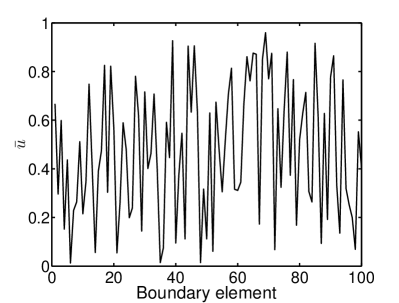
(a) Random $\bar{\mathbf{u}}$ as input

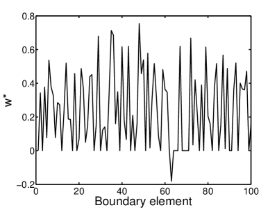
(b) Computed $\mathbf{w}^{*}_{\bar{\mathcal{I}}}$

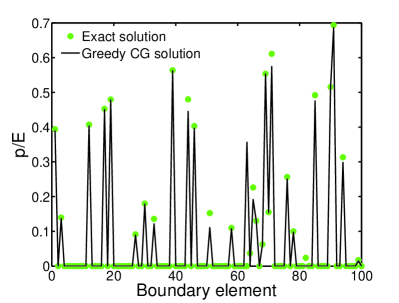
(c) Computed $\mathbf{p}/E$

Figure 2: Counterexample showing that the greedy CG method fails in getting the correct solution ($\delta=1$ a.u. of $L$, as $\mathbf{u}$ and $\mathbf{w}^{*}$; $E=0.01$ $F/L^{2}$). Green dots correspond to the correct contact forces satisfying the LCP and are obtained by using the NNLS method, Sec. 3.2

Therefore, as a word of caution, the reliability of the greedy method should be carefully checked in case of applications of BEM to contact problems governed by other forms of $\mathbf{H}$, as in the case of contact with an anisotropic or an inhomogeneous half-space, or in the presence of multiple fields.

Another drawback of the algorithm is the difficulty to warm start the method with a proper choice of the initial active set $\mathcal{I}$. Since at Step 2.5.1 the number of elements in the sequence $\mathcal{I}$ is decreased by removing negative enough components $\mathbf{p}_{j}$ of the current solution vector, i.e., eliminating the points bearing tensile (negative) forces, in a monotonic way (no index $j$ that has been removed from $\mathcal{I}$ can be added back), a safe cold start is to set $\mathcal{I}=\{1,\ldots,n\}$ and pick up a vector $\mathbf{p}\geq\textbf{0}$, usually a vector with arbitrary non-negative numbers. The history of contact forces obtained during the solution of a sequence of imposed displacements is not taken into account by the method to accelerate its convergence, although we know that contact forces are monotonically increasing functions of the far-field displacement. In any case, for a complex sequence of loading with an increased or decreased far-field displacement, any warm starting on forces cannot be implemented in the method, since the elimination of contact points is irreversible.

3.2 Constrained Conjugate Gradient

A constrained CG algorithm was proposed by Polonsky and Keer (1999) based on the theory by (Hestenes, 1980, Ch. 2,3) to solve the linear system of equations and rigorously impose the satisfaction of the contact constraints. Algorithm 2 has been applied by Polonsky and Keer (1999) to simulations under load control. However, it can be used also for displacement control. The condition for convergence set by Polonsky and Keer (1999) in terms of relative variation in the local contact forces from an iteration to the next has been recast in terms of the error in the local contact displacements. The two criteria are completely equivalent.

This constrained CG algorithm does not remove the points bearing tensile forces from the active set. Therefore, the size of the linear system of equations is not reduced during the iterations, increasing the computation time for its solution. On the other hand, the method assures the satisfaction of the LCP conditions (14) and it is found to convergence with a reduced number of iterations as compared to the Greedy CG algorithm. Although not investigated in (Polonsky and Keer, 1999), it can be warm started in case of a sequence of loading steps by considering both an initial trial contact domain and a set of contact pressures derived from the previous converged solution. The FFT method can be used to accelerate step (2.7) as in (Polonsky and Keer, 2000a).

Algorithm 2 Constrained Conjugate Gradient

    Input: Matrix $\mathbf{H}=\mathbf{H}^{\prime}\succ 0$, vector $\bar{\mathbf{u}}$, initial guess $\mathbf{p}\geq\mathbf{0}$, initial active set $\mathcal{I}=\{1,\ldots,n\}$; maximum number $K_{\rm max}$ of iterations, tolerance $\epsilon>0$.  

1. $i\leftarrow 0$, $n_{w,\rm{old}}=1$, $d=0$, $err=+\infty$;

2. $\mathbf{w}\leftarrow\mathbf{H}\mathbf{p}-\bar{\mathbf{u}}$;

3. while ($i\leq K_{\rm max}$ and $err>\epsilon$):

   1. if $i=0$  then $\mathbf{t}\leftarrow\mathbf{w}$  else: $\mathbf{t}\leftarrow\mathbf{w}+d\dfrac{n_{w}}{n_{w,\rm{old}}}\mathbf{t}_{\rm{old}}$;

   2. $\tau=\dfrac{\mathbf{w}^{\prime}\mathbf{t}}{\mathbf{t}^{\prime}\mathbf{H}\mathbf{t}}$;

   3. $\mathbf{p}\leftarrow\mathbf{p}-\tau\mathbf{t}$;

   4. $\forall j\in\mathcal{I}:p_{j}\leftarrow\max\{p_{j},0\}$;

   5. Find $I_{ol}=\{j\in\mathcal{I}:p_{j}=0,w_{j}<0\}$;
      if $I_{ol}=\emptyset$ then $d=1$ else $d=0$; $p_{j}\leftarrow p_{j}-\tau w_{j}$, $\forall j\in I_{ol}$;

   6. $\mathcal{I}\leftarrow\{j:p_{j}>0\}\cup I_{ol}$;

   7. $\mathbf{t}_{\rm{old}}\leftarrow\mathbf{t}$, $n_{w,\rm{old}}\leftarrow n_{w}$;

   8. $\mathbf{w}\leftarrow\mathbf{H}\mathbf{p}-\bar{\mathbf{u}}$;

   9. $n_{w}=\|\mathbf{w}\|_{2}$;

   10. $err\leftarrow|n_{w}-n_{w,\rm{old}}|/n_{w,\rm{old}}$;

   11. $i\leftarrow i+1$;

4. $\mathbf{p}^{*}\leftarrow\mathbf{p}$; $\mathbf{u}^{*}=\mathbf{H}\mathbf{p}^{*}$;

5. end.

    Output: Contact force vector $\mathbf{p}^{*}$ and normal displacement vector $\mathbf{u}^{*}$.  

3.3 Non-Negative Least Squares (NNLS)

In this section we show how a QP problem with positive definite Hessian matrix having the special form (16) can be effectively solved as a nonnegative least squares problem.

Thanks to property (15), matrix $\mathbf{H}$ admits a Cholesky factorization $\mathbf{H}=\mathbf{C}^{\prime}\mathbf{C}$. Hence we can theoretically recast problem (16) as the Non-Negative Least Squares (NNLS) problem:

$$\text{min}_{p} \;\dfrac{1}{2}\|\mathbf{C}\mathbf{p}-\mathbf{C}^{-T}\bar{\mathbf{u}}\|_{2}^{2}$$ (20a)

s.t. $$\mathbf{p}\geq\mathbf{0}$$ (20b)

A simple and effective active-set method for solving the NNLS problem (20) is the one in (Lawson and Hanson, 1974, p.161), that is extended here in Algorithm 3 to directly solve (16) without explicitly computing the Cholesky factor $\mathbf{C}$ and its inverse $\mathbf{C}^{-1}$ and to handle warm starts. After a finite number of steps, Algorithm 3 converges to the optimal contact force vector $\mathbf{p}^{*}$ and returns the normal displacement vector $\mathbf{u}^{*}$ whose components $p_{i,j}$, $u_{i,j}$ satisfy $p_{i,j}\geq 0$, $u_{i,j}\geq\bar{u}_{i,j}$, $(u_{i,j}-\bar{u}_{i,j})p_{i,j}=0$, and (13), $\forall(i,j)\in I_{C}$.

The method is easy to warm start in case of a loading scenario consisting of an alternating sequence of increasing or decreasing far-field displacements. The contact forces determined for a given imposed displacement are used to initialize vector $\mathbf{p}$. Due to the monotonicity of the contact solution, this initialization is certainly much closer to the optimal solution $\mathbf{p}^{*}$ than a zero vector. This usually significantly reduces the iterations of the method to convergence. Such a warm start has a fast implementation requiring a projection of the forces of the points belonging to $I_{C}^{*}(\Delta_{k})$ to the same points of the trial domain $I_{C}^{*}(\Delta_{k+1})$ for a new imposed far field displacement $\Delta_{k+1}$. For an increasing far-field displacement, i.e., $\Delta_{k+1}>\Delta_{k}$ the forces in the elements belonging to $I_{C}^{*}(\Delta_{k+1})-I_{C}^{*}(\Delta_{k})$ are simply initialized equal to zero. In the numerical experiments of Section 4, the time required for this projection will be added to the global solution time for a consistent comparison with the greedy method with cold start and with the constrained CG algorithm.

Algorithm 3 Non-Negative Least Squares (NNLS)

    Input: Matrix $\mathbf{H}=\mathbf{H}^{\prime}\succ 0$, vector $\bar{\mathbf{u}}$, initial guess $\mathbf{p}$; maximum number $K_{\max}$ of iterations, tolerance $\epsilon>0$.  

1. $\mathcal{I}\leftarrow\{i\in\{1,\ldots,n\}:\ \mathbf{p}_{i}>\mathbf{0}\}$; $init\leftarrow\textsc{FALSE}$; $k\leftarrow 0$;

2. if $\mathcal{I}=\emptyset$ then $init\leftarrow\textsc{TRUE}$;

3. $\mathbf{w}\leftarrow\mathbf{H}\mathbf{p}-\bar{\mathbf{u}}$;

4. if (($\mathbf{w}\geq-\epsilon$ or $\mathcal{I}=\{1,\ldots,n\}$) and $init=\textsc{TRUE}$) or $k\geq K_{\max}$ then go to Step 13;

5. if $init=\textsc{TRUE}$ then $i\leftarrow\arg\min_{i\in\{1,\ldots,n\}\setminus\mathcal{I}}\mathbf{w}_{i}$; $\mathcal{I}\leftarrow\mathcal{I}\cup\{i\}$;
   else $init\leftarrow\textsc{TRUE}$;

6. $\mathbf{s}_{I}\leftarrow$ solution of the linear system $\mathbf{H}_{I}\mathbf{s}_{I}=\bar{\mathbf{u}}_{I}$

7. if $\mathbf{s}_{\mathcal{I}}\geq-\epsilon$ then $\mathbf{p}\leftarrow\mathbf{s}$ and go to Step 3;

8. $j\leftarrow\arg\min_{h\in\mathcal{I}:\ \mathbf{s}_{h}\leq\mathbf{0}}\left\{\frac{\mathbf{p}_{h}}{\mathbf{p}_{h}-\mathbf{s}_{h}}\right\}$;

9. $\mathbf{p}\leftarrow\mathbf{p}+\frac{\mathbf{p}_{j}}{\mathbf{p}_{j}-\mathbf{s}_{j}}(\mathbf{s}-\mathbf{p})$;

10. $\mathcal{I}_{0}\leftarrow\{h\in\mathcal{I}:\mathbf{p}_{h}=\mathbf{0}\}$;

11. $\mathcal{I}\leftarrow\mathcal{I}\setminus\mathcal{I}_{0}$; $k\leftarrow k+1$;

12. go to Step 6;

13. $\mathbf{p}^{*}\leftarrow\mathbf{p}$;

14. $\mathbf{u}^{*}\leftarrow\mathbf{w}+\bar{\mathbf{u}}$;

15. end.

    Output: Contact force vector $\mathbf{p}^{*}$ and normal displacement vector $\mathbf{u}^{*}$ satisfying $\mathbf{u}^{*}=\mathbf{H}\mathbf{p}$, $\mathbf{u}^{*}\geq\bar{\mathbf{u}}$, $\mathbf{p}^{*}\geq\mathbf{0}$, $(\mathbf{u}^{*}-\bar{\mathbf{u}})^{\prime}\mathbf{p}=0$.  

Note that Step 6 of Algorithm 3 is equivalent to Step 2.4 of Algorithm 1 and has been performed by using the MATLAB’s mldivide solver. This step can be accelerated by the use of an approach based on the FFT (for its implementation, see e.g. (Batrouni et al., 2002)). Alternatively, since the set $\mathcal{I}_{0}$ changes incrementally during the iterations of the algorithm, more efficient iterative QR (Lawson and Hanson, 1974, Chap. 24) or LDL^T Bemporad (2014) factorization methods can be employed.

3.3.1 Warm-started NNLS via accelerated Gradient Projection (NNLS+GP)

An alternative method to solve Problem (16) is to use an accelerated gradient projection (GP) method for QP (Nesterov, 1983; Patrinos and Bemporad, 2014). Because of the simple nonnegative constraints in (16), rather than going to the dual QP formulation as in (Patrinos and Bemporad, 2014), we formulate the GP problem directly for the primal QP problem (16). Numerical experiments have shown slow convergence of a pure accelerated GP method to solve (16). However, we can use the method to warm start Algorithm 3, as described in Algorithm 4. If Algorithm 4 is executed $(K>0)$, it returns a vector $\mathbf{p}$ that is immediately used as an input to Algorithm 3, otherwise one can simply set $\mathbf{p}=\mathbf{0}$ (cold start). As shown in Section 4, GP iterations provide large benefits in warm starting the NNLS solver, therefore allowing taking the best advantages of the two methods: quickly getting in the neighborhood of the optimal solution (GP iterations of Algorithm 4) and getting solutions up to machine precision after a finite number of iterations (the active-set NNLS Algorithm 3).

Algorithm 4 Accelerated Gradient Projection (GP)

    Input: Matrix $\mathbf{H}=\mathbf{H}^{\prime}\succ 0$ and its Frobenius norm $L$, vector $\bar{\mathbf{u}}$, initial guess $\mathbf{p}$, number $K$ of iterations.  

1. $\bar{\mathbf{p}}\leftarrow\mathbf{p}$;

2. for $i=0,\ldots,K-1$ do:

   1. $\beta=\max\{\frac{i-1}{i+2},0\}$;

   2. $\mathbf{s}=\mathbf{p}+\beta(\mathbf{p}-\bar{\mathbf{p}})$;

   3. $\mathbf{w}=\mathbf{H}\mathbf{s}-\bar{\mathbf{u}}$;

   4. $\bar{\mathbf{p}}\leftarrow\mathbf{p}$;

   5. $\mathbf{p}\leftarrow\max\{\mathbf{s}-\frac{1}{L}\mathbf{w},\mathbf{0}\}$;

3. end.

    Output: Warm start for contact force vector $\mathbf{p}$ and elastic correction vector $\mathbf{w}$.  

3.4 Alternating Direction Method of Multipliers (ADMM)

The QP problem (16) can also be solved by the Alternating Direction Method of Multipliers (ADMM), which belongs to the class of augmented Lagrangian methods. The reader is referred to  (Boyd et al., 2011) for mathematical details. The method treats the QP (16) as the following problem

$$\begin{array}[]{rl}\min_{\mathbf{p},\mathbf{s}}&\frac{1}{2}\mathbf{p}^{\prime}\mathbf{H}\mathbf{p}-\bar{\mathbf{u}}^{\prime}\mathbf{p}+g(\mathbf{s})\\ {\rm s.t.}&\mathbf{p}=\mathbf{s}\end{array}$$ (21)

where

$$g(\mathbf{s})=\left\{\begin{array}[]{rcl}0&\mbox{if}&\mathbf{s}\geq\mathbf{0}\\ +\infty&\mbox{if}&\mathbf{s}<\mathbf{0}\end{array}\right.$$

Then, the augmented Lagrangian function

$$L_{\rho}(\mathbf{p},\mathbf{s},\mathbf{w})=\frac{1}{2}\mathbf{p}^{\prime}\mathbf{H}\mathbf{p}-\bar{\mathbf{u}}^{\prime}\mathbf{p}+g(\mathbf{s})+\mathbf{w}^{\prime}(\mathbf{p}-\mathbf{s})+\frac{\rho}{2}\|\mathbf{p}-\mathbf{s}\|_{2}^{2}$$

is considered, where $\rho>0$ is a parameter of the algorithm. The basic ADMM algorithm consists of the following iterations:

$$\begin{array}[]{rcl}\mathbf{p}^{k+1}&=&\arg\min_{\mathbf{p}}L_{\rho}(\mathbf{p},\mathbf{s}^{k},\mathbf{w}^{k})\\ \mathbf{s}^{k+1}&=&\arg\min_{\mathbf{s}}L_{\rho}(\mathbf{p}^{k+1},\mathbf{s},\mathbf{w}^{k})\\ \mathbf{w}^{k+1}&=&\mathbf{w}^{k}+\rho(\mathbf{p}^{k+1}-\mathbf{s}^{k+1})\end{array}$$ (22)

A scaled form with over-relaxation of the ADMM iterations (22) is summarized in Algorithm 5. The algorithm is guaranteed to converge asymptotically to the solution $\mathbf{p}^{*}$, $\mathbf{u}^{*}$ of the problem. The over-relaxation parameter $\alpha>1$ is introduced to improve convergence, typical values for $\alpha$ suggested in (Boyd et al., 2011) are $\alpha\in[1.5,1.8]$.

A warm start of the algorithm that takes into account the loading history is possible in a way analogous to that described for the NNLS approach of Section 3.3. However, as an additional complexity, also an initialization for the dual variable vector $\mathbf{w}$ must be provided, possibly obtained by projecting the solution obtained for a certain $\Delta_{k}$ to that for $\Delta_{k+1}$.

Algorithm 5 Alternative Direction Method of Multipliers (ADMM)

    Input: Matrix $\mathbf{H}=\mathbf{H}^{\prime}\succ 0$, vector $\bar{\mathbf{u}}$, initial guesses $\mathbf{p}$, $\mathbf{w}$, parameter $\rho>0$, over-relaxation parameter $\alpha>1$, maximum number $K_{\rm max}$ of iterations, tolerance $\epsilon>0$.  

1. $\mathbf{M}\leftarrow(\frac{1}{\rho}\mathbf{H}+\mathbf{I})^{-1}$;

2. $\mathbf{w}_{\rho}\leftarrow-\frac{1}{\rho}\mathbf{w}$;

3. $\mathbf{s}\leftarrow\mathbf{p}$;

4. $i\leftarrow 0$;

5. while ($i\leq K_{\rm max}$ and $\|\mathbf{p}-\mathbf{s}\|_{\infty}>\epsilon$) or $i=0$ do:

   1. $\mathbf{s}\leftarrow\mathbf{M}(\mathbf{p}-\mathbf{w}_{\rho}-\frac{1}{\rho}\bar{\mathbf{u}})$;

   2. $\bar{\mathbf{s}}\leftarrow\alpha\mathbf{s}+(1-\alpha)\mathbf{p}$;

   3. $\mathbf{p}\leftarrow\max\{\bar{\mathbf{s}}+\mathbf{w}_{\rho},\mathbf{0}\}$;

   4. $\mathbf{w}_{\rho}\leftarrow\mathbf{w}_{\rho}+\bar{\mathbf{s}}-\mathbf{p}$;

   5. $i\leftarrow i+1$;

6. $\mathbf{p}^{*}\leftarrow\mathbf{p}$;

7. $\mathbf{u}^{*}\leftarrow\bar{\mathbf{u}}-\rho\mathbf{w}_{\rho}$;

8. end.

    Output: Contact force vector $\mathbf{p}^{*}$ and normal displacement vector $\mathbf{u}^{*}$ satisfying $\mathbf{u}^{*}=\mathbf{H}\mathbf{p}$, $\mathbf{u}^{*}\geq\bar{\mathbf{u}}$, $\mathbf{p}^{*}\geq\mathbf{0}$, $(\mathbf{u}^{*}-\bar{\mathbf{u}})^{\prime}\mathbf{p}=0$.  

4 Performance comparison of the algorithms

The optimization algorithms presented in the previous section are herein applied to the frictionless normal contact problem between a numerically generated pre-fractal rough surface and a half-plane, in order to compare their performance in terms of number of iterations required to achieve convergence and computation time.

The random midpoint displacement algorithm (Peitgen and Saupe, 1988) is used to generate the synthetic height field of surfaces with multiscale fractal roughness, i.e., with a power spectral density (PSD) function of the height field of power-law type. The surface with a given resolution (pre-fractal) is realized by a successive refinement of an initial coarse representation by adding a sequence of intermediate heights whose elevation is extracted from a Gaussian distribution with a suitable rescaled variance, see a qualitative sketch in Fig. 3. Several applications of the method to model rough surfaces for contact mechanics simulations are available in (Zavarise et al., 2004, 2007; Paggi and Ciavarella, 2010).

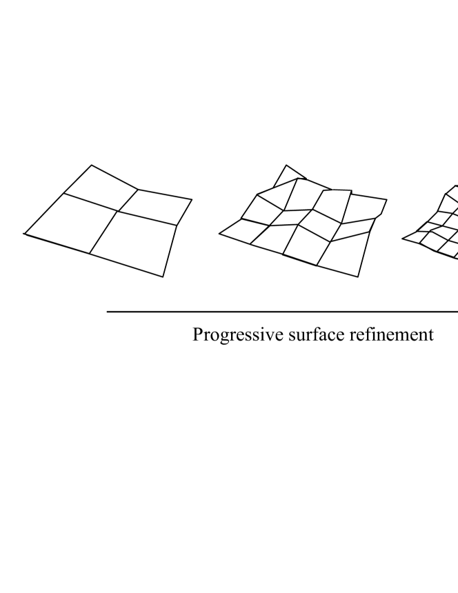
Figure 3: Rough surfaces with multi-scale roughness and different resolution, numerically generated by the random midpoint displacement algorithm.

In particular, we consider a test problem consisting of a surface with Hurst exponent $H=0.7$, lateral size $L=100$ $\mu$m and 512 heights per side, which corresponds to the highest discretization used to sample real surfaces with a confocal profilometer, like the Leica DCM3D available at the Multi-scale Analysis of Materials (MUSAM) Laboratory of IMT Lucca, Italy. Similar discretizations are obtained in case of AFM. The surface is brought into contact with an elastic half-plane under displacement control. Ten displacement steps are imposed to reach a maximum far-field displacement which is set equal to $(\xi_{\max}-\xi_{\text{ave}})/2$, where $\xi_{\max}$ and $\xi_{\text{ave}}$ are the maximum and the average elevations of the rough surface, respectively. All the simulations are carried out with the server 653745-421 Proliant DL585R07 from Hewlett Packard with 128 GB Ram, 4 processors AMD Opteron 6282 SE 2.60 GHz with 16 cores running MATLAB R2014b.

The parameters for the Greedy CG method are the maximum number of iterations $K_{\max}=1\times 10^{5}$ and the convergence tolerance $\epsilon=1\times 10^{-8}$. The contact forces are initialized at zero (cold start). The constrained CG method also considers $K_{\max}=1\times 10^{5}$ and the same tolerance $\epsilon=1\times 10^{-8}$. Both the original version by Polonsky and Keer (1999) (labeled P&K1999 in Fig. 4) and its warm-started variant (labeled P&K1999 + warm start in Fig. 4) are considered.

For the NNLS algorithm (Algorithm 3) we adopt the warm start strategy based on the projection of contact forces from the solution corresponding to a previous displacement step. Alternatively, for NNLS+GP, 100 gradient projections are used to initialize vector $\mathbf{p}$. For the ADMM method we use $\alpha=1.5$, $\rho=1$, $K_{\max}=3\times 10^{3}$ and $\epsilon=10^{-8}$. The total number $n$ of optimization variables is varying with $\Delta$ and therefore with the force level. For the highest indentation we have $n=35555$. Warm starting the algorithm is achieved by projecting primal variables as for the NNLS and dual variables $\mathbf{w}$ as well. The projection simply consists of assigning the values of $p_{i,j}^{*}$ and $w^{*}$ of the boundary elements in contact for the step $\Delta_{k}$ to the same boundary elements belonging to the trial contact domain $I_{C}$ corresponding to the higher indentation $\Delta_{k+1}$.

Once convergence is achieved for each imposed far-field displacement, the optimization algorithms provide the same normal force $P$ and contact domains, with small roundoff errors due to finite machine precision. The CPU time required by each method to achieve convergence are shown in Fig. 4 vs. the dimensionless normal force $P/(EA)$, where $E$ is the Young’s modulus and $A=L^{2}$ is the nominal contact area. The best performance is achieved by the application of the NNLS method with 100 gradient projections (GP), which is 26 times faster than the original constrained CG method by Polonsky and Keer (1999) and about two orders of magnitude faster than the ADMM and the Greedy CG algorithms.

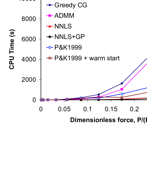
Figure 4: Comparison between the optimization algorithms in terms of computation time.

As outlined in the introduction, the Greedy method can be used in conjunction with other algorithms for solving the unconstrained linear system of equations (Step 2.4) than the CG algorithm. Although an extensive comparison of different solvers of linear systems of equations with positive definite matrices is outside the scope of this paper, we tested the Greedy algorithm after replacing the CG Step 2.4 with the optimized built-in mldivide function of MATLAB, or with the Gauss-Seidel algorithm, as proposed in Borri-Brunetto et al. (1999, 2001).

The MATLAB’s mldivide solver (which employs the Cholesky factorization) leads to a reduction of computation time of $30-40\%$, almost regardless of the size of the system $n$, see Fig. 5. Even with this gain in computation speed, the overall performance is still quite far from that of the NNLS Algorithm 3 on the platform used for the tests. Moreover, the MATLAB solver leads to an error of lack of memory for $n>20000$, a serious problem for large systems that is not suffered by the CG solver described in Step 2.4 of Algorithm 1. The Gauss-Seidel algorithm does not suffer for the lack of memory but it is about 3 times slower than the CG method.

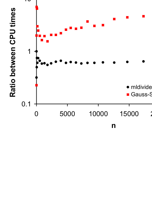
Figure 5: Computation times for the Greedy method for different sizes $n$ of the contact superset $I_{C}$: CG vs. MATLAB’s mldivide solver and CG vs. Gauss-Seidel algorithm.

The effect of the number $K$ of GP iterations applied before the NNLS algorithm is investigated in Fig. 6 for the same test problem whose results were shown in Fig. 4. By increasing $K$ from 0 to 100 we observe a reduction in the total computation time due to a decrease in the number of iterations requested by the NNLS algorithm to achieve convergence thanks to a better initial guess of $\mathbf{p}$. However, a further increase in $K$ (see, e.g., the blue curve in Fig. 6 corresponding to $K=200$ iterations) does not correspond to further savings of CPU time. This is due to the fact that the number of NNLS iterations was already reduced to its minimum for $K=100$ GP iterations, so that the application of further gradient projections are just leading to additional CPU time without further benefit.

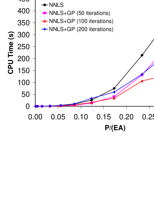
Figure 6: Computation times of the NNLS algorithm depending on the number $K$ of gradient projection (GP) iterations.

5 Cascade multi-resolution (CMR) method

5.1 Algorithm

A further speed-up of computation time, as compared to the NNLS method, can be achieved by improving the criterion for the guess of the initial set $I_{C}$ of points in contact. The standard criterion based on checking the interpenetration of the surface heights into the half-plane in case of a rigid body motion is the most conservative. However, at convergence, only a small subset $I_{C}^{*}$ of that initial set is actually in contact. Therefore, a better choice of the initial trial contact domain would reduce the size of the system of linear equations with an expected benefit in terms of computation time.

As shown in (Borri-Brunetto et al., 1999) via numerical simulations on pre-fractal surfaces with Hurst exponent $H>0.5$ and different resolution, by refining the surface height field via a recursive application of the random midpoint displacement algorithm the real contact area of each surface representation decreases by reducing $\delta$, as illustrated in the sketch in Fig. 7. In the fractal limit of $\delta\to 0$, the real contact area vanishes. Therefore, this property of lacunarity implies that the heights that are not in contact for a coarser surface representation are not expected to come into contact by a successive refining of the height field, for the same imposed far-field displacement.

Therefore, as a better criterion, the initial trial contact domain can be selected by retaining, among all the heights selected by the rigid body interpenetration check, only those located within the areas of influence of the nodes belonging to the contact domain of a coarser representation of the rough surface for the same imposed displacement $\Delta$.

As graphically shown in Fig. 7, an area of influence of a given node in contact can be defined by the radius $\sqrt{2}\delta$, where $\delta$ is the grid size of the coarser surface representation. Since the criterion is not exact, it is convenient to consider a multiplicative factor $h$ larger than one for the radius defining the nodal area of influence. It is remarkable to note that this numerical scheme can be applied recursively to a cascade of coarser representations of the same rough surface. As a general trend, computation time is expected to drastically diminish by increasing the number of cascade projections. However, the propagation of errors due to the wrong exclusion of heights that would actually make contact cannot be controlled by the algorithm and it is expected to increase with the number of projections as well. The advantage of the method is represented by the fact that, in addition to saving computation time with respect to that required by the NNLS algorithm to solve just the contact problem for the finest surface, all the contact predictions for the coarser scale representations of the same surface will be available for free, which is a useful result for the multi-scale characterization of contact problems. Moreover, the CMR method can be used in conjunction with any of the optimization algorithms presented in the previous sections.

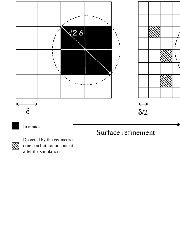
Figure 7: A sketch illustrating the property of lacunarity of the contact domain: the real contact area progressively diminishes by refining the surface, until vanishes in the fractal limit of $\delta\to 0$. This implies that some boundary elements detected by the rigid-body interpenetration criterion (dashed grey elements) can be neglected a priori since they are outside the real contact area corresponding to the coarse scale contact solution.

The algorithm is illustrated in Algorithm (6).

Algorithm 6 Cascade multi-resolution (CMR) algorithm

    Input: $s=1,\dots,l$ surface representations with different resolution or grid spacing $\delta(s)$; area of influence parameter $h\geq 1$.  

1. for $s=1,\dots,l$ do:

   1. Determine $I_{C}(s)=\{(i,j)\in I_{N}(s):\xi_{i,j}\geq\xi_{\max}(s)-\Delta\}$;

   2. if $s=1$ then $I_{C,p}(s)=I_{C}(s)$
      else $I_{C,p}(s)=\{(i,j)\in I_{C}(s):r_{i-k,j-l}=\|\mathbf{x}_{i,j}-\mathbf{x}_{k,l}\|\leq h\delta(s-1)\}$, $\forall(k,l)\in I_{C}^{*}(s-1)$
      end

2. Construct $\mathbf{H}$ based on the projected trial contact domain $I_{C,p}(s)$;

3. Apply optimization algorithms (e.g., NNLS) and determine $\mathbf{p}^{*}$, $\mathbf{u}^{*}$, $I_{C}^{*}(s)$;

4. end.

 

5.2 Validation in case of numerically generated and real rough surfaces

To assess the computational performance of the approach described in Section 5.1, the CMD method is applied in conjunction with the NNLS algorithm to pre-fractal surfaces with different $H$ numerically generated by the RMD method. As an example, the lateral size is $100$ $\mu$m for all the surfaces and the finest resolution whose contact response has to be sought corresponds to 256 heights per side. The method requires the storage of the coarser representations of such surfaces that are in any case available by the RMD algorithm during its various steps of random addition.

We apply the cascade of projections starting by a coarser representation of the surfaces with only 16 heights per side and then considering 32, 64, 128 and finally 256 heights per side. A parameter $h=2$ has been used for the definition of the area of influence. The solution of the contact problem for the surface with 16 heights per side is obtained in an exact form since it is the starting point of the cascade, whereas the contact predictions for the finer surface representations can be affected by an error intrinsic in the criterion. The approximate predictions for the surface with 256 heights per side are compared with the reference solution corresponding to the application of the NNLS algorithm with warm start directly to the finest representation of the rough surface.

The computation time of the CMR+NNLS solution is the sum of the CPU time required to solve all the coarser surface representations and it is found to be much less than the CPU time required by the NNLS algorithm to solve just one single surface with the finest resolution, see Fig. 8, where we observe a reduction of $50\%$ in CPU time almost regardless of $H$. The relative error in the computation of the maximum normal force between the predicted solution and the reference one is a rapid decreasing function of $H$, as shown in Fig. 8(d). Considering that real surfaces have often a Hurst exponent $H>0.5$, this is very promising.

A synthetic diagram illustrating the effect of the parameter $h$ for the surface with $H=0.7$ and for a single imposed displacement corresponding to the maximum load in Fig. 8(c) is shown in Fig. 9. The relative error is rapidly decreasing to values less than $1\%$ by increasing $h$. The ratio between the number of points expected to be in contact after the application of the CMR projection criterion, $n_{p}$, and the number of points that would be included by using the classic rigid-body interpenetration check, $n$, is ranging from 0.4 to 0.8 by increasing $h$ from 1.25 to 3.0. The ratio between CPU times, on the other hand, tends to an asymptotic value of 0.6, which implies a saving of 40% of computation time as compared to the exact solution, with less than 0.01% of relative error.

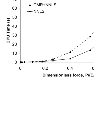
(a) $H=0.3$

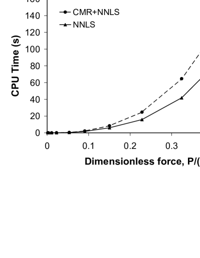
(b) $H=0.5$

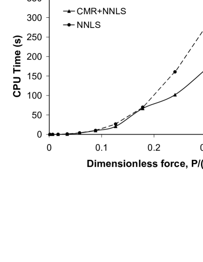
(c) $H=0.7$

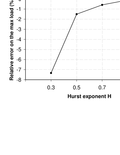
(d) Relative error

Figure 8: Performance of the CMR+NNLS method applied to numerically generated fractal surfaces with different Hurst exponent $H$, $h=2$.

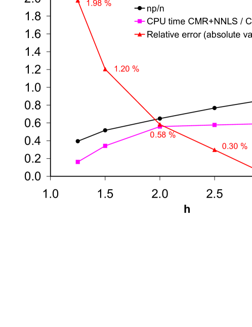
Figure 9: Performance of the CMR+NNLS method with respect to NNLS for a numerically generated fractal surface with $H=0.7$, depending on the parameter $h$.

We also check the CMR method for warm starting on real surfaces not displaying the ideal fractal scaling at any length scale, to better assess possible limits of applicability. As a practical example we consider the surface of textured silicon solar cells sampled with two different lenses in order to achieve two different magnifications (10x and 100x) by using the confocal profilometer Leica DCM3D, see Fig. 10. The PSD function of such a surface sampled with 512 points per side presents a power-law trend for high frequencies (fine resolutions) and a cut-off to the power-law at low frequencies (coarse resolutions). In the power-law regime the surface is characterized by a Hurst exponent $H\cong 0.6$ that can be determined by the slope of the PSD function as customary.

As a main difference with respect to pre-fractal rough surfaces generated by the RMD algorithm, the application of the CMR method requires a filter to downsample the acquired surfaces and extract their coarser representations. The CMR method is applied to the two surfaces acquired with 10x and 100x magnifications using $h=1.5$ and considering a cascade of projections involving coarser representations of the finest surfaces with 64 and 128 heights per side. A single contact step corresponding to an imposed far-field normal displacement equal to $(\xi_{\max}-\xi_{\text{ave}})/5$ is examined.

The application of the CMR+NNLS method to the surface acquired at 100x leads to very good results in line with those observed for ideal fractal surfaces. The relative error in the prediction of the normal load is $-0.4\%$, with a saving of CPU time of $18\%$ as compared to the direct application of the NNLS algorithm. On the other hand, the method applied to the surface acquired at 10x leads to poor results in terms of accuracy with $-98\%$ of relative error and almost no saving in computation time. This bad performance is due to the fact that the property of lacunarity of the contact domain, strictly connected with the self-affine scaling of roughness due to fractality, does not hold anymore for the surface sampled at 10x due to the cut-off to its power-law PSD. As a consequence, the CMR method erroneously excludes many possible points from the initial contact domain suggested by the rigid body interpenetration check that are actually relevant for contact. Therefore, in conclusion, the CMR method is efficient for warm starting the NNLS algorithm, but it should be strictly applied to numerically generated or real rough surfaces provided that the self-affine properties of roughness are confirmed by a PSD function of power-law type.

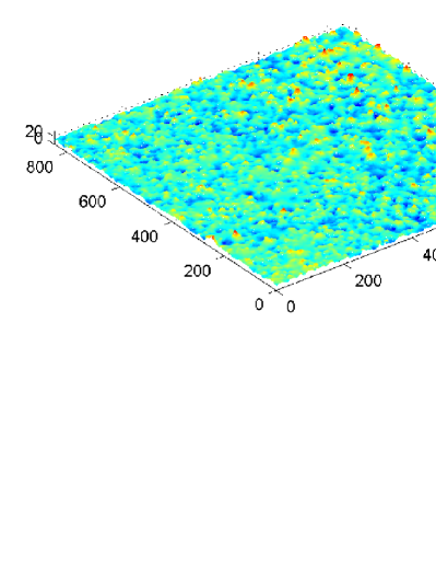
(a) 10x

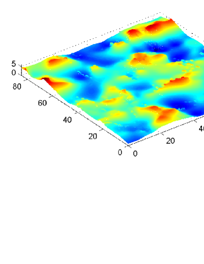
(b) 100x

Figure 10: Surface of textured silicon solar cells sampled with a confocal profilometer at two different magnifications (10x and 100x) obtained by using two different lenses.

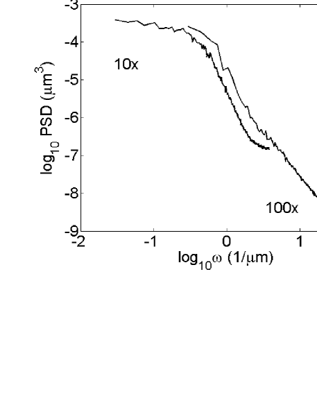
Figure 11: Power spectral density function (PSD) of the two sampled rough surfaces shown in Fig. 10.

6 Conclusion

This paper has shown how the problem of frictionless normal contact between rough surfaces within the BEM framework can be solved very efficiently by exploiting ideas from convex quadratic programming. A series of efficient optimization algorithms has been proposed and compared with the traditional Greedy method and constrained CG algorithm. As the lack of convergence of the Greedy method seems to be a rare phenomenon, it remains an open question to establish the conditions on $\mathbf{H}$ and $\bar{\mathbf{u}}$ for which the algorithm is guaranteed to converge.

The NNLS algorithm warm started by accelerated gradient projections was shown at least two orders of magnitude faster than the Greedy method and 26 times faster than the original constrained CG algorithm.

Finally, we explored another method for warm starting the optimization algorithms, this time focusing on a selective reduction of the size of the initial trial contact domain based on the multi-resolution properties of roughness. The resulting cascade multi-resolution (CMR) method allows a further saving of about $50\%$ of CPU time as compared to NNLS for contact simulations involving numerically generated fractal surfaces. Relative errors were found less than $2\%$ for surfaces with $H>0.5$, by using $h=2$, that was found a good compromise between accuracy and computation time. Moreover, it has to be remarked that not only the solution of the finest contact problem is gained by the CMR+NNLS method with much less CPU time, but also the contact problems involving all the coarser representations of the finest surface. These results are particularly important for speeding up intensive Monte Carlo simulations involving a sequence of contact simulations for a population of fractal surface with different resolution. So far, to the best of the authors’ knowledge, such extensive simulations, that are important to determine more reliable trends from the statistical point of view, have been limited to populations of 20 to 50 randomly generated surfaces.

In case of real surfaces, a very good performance (less than $2\%$ of error with 3 cascades and at least 18$\%$ of CPU time saved for one single imposed displacement step) has been demonstrated in case of power-law PSDs, assuring the self-affine scaling of roughness which represents the main underlying assumption for the algorithm applicability. For surfaces with a cut-off to the power-law PSD, on the other hand, the CMR+NNLS method has given poor results in terms of accuracy and in any case almost no saving in CPU time as compared to the pure application of NNLS. Therefore, this warm start method should be used with care and only in a range where the PSD is of power-law type.

Finally, we point out that the proposed optimization methods can also be applied to frictional contact problems by using for instance the complete BEM formulation as in (Pohrt and Li, 2014). Although this issue is left for further investigation, we expect an even more significant gain in CPU time by applying the algorithms presented in this paper instead of other optimization methods, since the size of the problem is by far significantly increased as compared to the frictionless case.

Acknowledgements

The research leading to these results has received funding from the European Research Council under the European Union’s Seventh Framework Programme (FP/2007-2013) / ERC Grant Agreement n. 306622 (ERC Starting Grant “Multi-field and multi-scale Computational Approach to Design and Durability of PhotoVoltaic Modules” - CA2PVM; PI: Prof. M. Paggi).

References

- Andersson (1981) T. Andersson, The Boundary Element Method applied to Two-Dimensional Contact Problems with Friction, In: Boundary Element Methods 3 (1981) 239–258.
- Barber (1974) J.R. Barber, Determining the contact area in elastic-indentation problems, Journal of Strain Analysis 9 (1974) 230–232.
- Barber (2003) J.R. Barber, Bounds on the electrical resistance between contacting elastic rough bodies, Proceedings of the Royal Society of London, Ser. A 459 (2003) 53–66.
- Barber (2010) J.R. Barber, Elasticity, Springer, Dordrecht, 3rd Edition, 2010.
- Batrouni et al. (2002) G.G. Batrouni, A. Hansen, J. Schmittbuhl, Elastic response of rough surfaces in partial contact, Europhysics Letters 60 (2002) 724–730.
- Beale (1955) E.M.L. Beale, On minimizing a convex function subject to linear inequalities, Journal of the Royal Statistical Society, Ser. B (1955) 173–184.
- Bemporad (2014) A. Bemporad, A quadratic programming algorithm based on nonnegative least squares with applications to embedded model predictive control, IEEE Trans. Autom. Control. Conditionally accepted for publication (2014).
- Borri-Brunetto et al. (1999) M. Borri-Brunetto, A. Carpinteri, B. Chiaia, Scaling phenomena due to fractal contact in concrete and rock fractures, International Journal of Fracture 95, (1999) 221–238.
- Borri-Brunetto et al. (2001) M. Borri-Brunetto, B. Chiaia, M. Ciavarella, Incipient sliding of rough surfaces in contact: a multiscale numerical analysis, Computer Methods in Applied Mechanics and Engineering 190 (2001) 6053–6073.
- Boyd et al. (2011) S. Boyd, N. Parikh, E. Chu, B. Peleato, and J. Eckstein, Distributed optimization and statistical learning via the alternating direction method of multipliers, Foundations and Trends in Machine Learning 3 (2011) 1–122.
- Campaña et al. (2011) C. Campana, B.N.J. Persson, M.H. Müser, Transverse and normal interfacial stiffness of solids with randomly rough surfaces, Journal of Physiscs: Condensed Matter 23 (2001) 085001.
- Carbone and Bottiglione (2008) G. Carbone, F. Bottiglione, Asperity contact theories: Do they predict linearity between contact area and load?, Journal of the Mechanics and Physics of Solids 56 (2008) 2555–2572.
- Carbone and Putignano (2013) G. Carbone, C. Putignano, A novel methodology to predict sliding and rolling friction of viscoelastic materials: theory and experiments, Journal of the Mechanics and Physics of Solids 61 (2013) 1822–1834.
- Ciavarella et al. (2006) M. Ciavarella, V. Delfine, G. Demelio, A “re-vitalized” Greenwood & Williamson model of elastic contact between fractal surfaces, Journal of the Mechanics and Physics of Solids 54 (2006) 2569–2591.
- Ciavarella et al. (2008a) M. Ciavarella, S. Dibello, G. Demelio, Conductance of rough random profiles, International Journal of Solids and Structures 45 (2008) 879–893.
- Ciavarella et al. (2008b) M. Ciavarella, J.A. Greenwood, M. Paggi, Inclusion of “interaction” in the Greenwood and Williamson contact theory, Wear 265 (2008) 729–734.
- Cottle et al. (1992) R.W. Cottle, J.-S. Pang, R.E. Stone, The Linear Complementarity Problem, Academic Press (1992).
- Fletcher (1971) R. Fletcher, A general quadratic programming algorithm, IMA Journal of Applied Mathematics, 7 (1971) 76-91.
- Francis (1983) H.A. Francis, The accuracy of plane strain models for the elastic contact of three-dimensional rough surfaces, Wear, 85 (1983) 239-256.
- Goldfarb and Idnani (1983) D. Goldfarb and A. Idnani, A numerically stable dual method for solving strictly convex quadratic programs, Mathematical Programming 27(1) (1983) 1–33.
- Hestenes (1980) M.R. Hestenes, Conjugate Direction Methods in Optimization, Springer, New York, Ch. 2 and 3 (1980).
- Hendriks and Visscher (1995) C.P. Hendriks and M. Visscher. Accurate real area of contact measurements on polyuretane, ASME Journal of Tribology 117 (1995) 607–611.
- Hyun et al. (2004) S. Hyun, L. Pei, J.-F. Molinari, M.O. Robbins, Finite-element analysis of contact between elastic self-affine surfaces, Physical Review E 70 (2004) 026117.
- Hyun and Robbins (2007) S. Hyun, M.O. Robbins Elastic contact between rough surfaces: effect of roughness at large and small wavelengths, Tribolology International 40 (2007) 1413.
- Johnson (1985) K.L. Johnson, Contact Mechanics, Cambridge University Press, Cambridge, UK, 1985.
- Kalker and van Randen (1972) J.J. Kalker and Y.A. van Randen, A minimum principle for frictionless elastic contact with application to non Hertzian problems, Journal of Engineering Mathematics 6 (1972) 193–206.
- Karpenko and Akay (2001) Y.A. Karpenko, A. Akay, A numerical model of friction between rough surfaces, Tribology International 34 (2001) 531–545.
- Kubo et al. (1981) A. Kubo, T. Okamoto, N. Kurokawa, Contact stress between rollers with surface irregularity, Journal of Tribology 116 (1981) 492–498.
- Lawson and Hanson (1974) C. Lawson and R. Hanson, Solving Least Squares Problems, SIAM 161 (1974), Ch. 24.
- Li and Berger (2003) J. Li and E.J. Berger, A semi-analytical approach to three-dimensional normal contact problems with friction, Computational Mechanics 30 (2003) 310-322.
- Man (1994) K.W. Man, Contact Mechanics Using Boundary Elements, Topics in Engineering, Vol. 22, Computational Mechanics Publications, Southampton, Boston, 1994.
- McCool (1986) J.I. McCool, Comparison of models for the contact of rough surfaces, Wear 107 (1986) 37–60.
- Nesterov (1983) Y. Nesterov, A method of solving a convex programming problem with convergence rate , Soviet Mathematics Doklady 27 (1983) 372–376.
- Nogi and Kato (1997) T. Nogi and T. Kato, Influence of a hard surface layer on the limit of elastic contact – Part I: analysis using a real surface model, Journal of Tribology 110 (1998) 493–500.
- Nosonovsky and Bhushan (2005) M. Nosonovsky, B. Bhushan, Roughness optimization for biomimetic superhydrophobic surfaces, Microsystem Technologies 11 (2005) 535–549.
- O’Callaghan and Probert (2005) P.W. O’Callaghan and S.D. Probert, Real area of contact between a rough surface and a softer optically flat surface, Journal of Mechanical Engineering Science 11 (1970) 259–267.
- Paggi and Barber (2011) M. Paggi, J.R. Barber, Contact conductance of rough surfaces composed of modified RMD patches, International Journal of Heat and Mass Transfer 54 (2011) 4664–4672.
- Paggi and Ciavarella (2010) M. Paggi, M. Ciavarella, The coefficient of proportionality between real contact area and load, with new asperity models, Wear 268 (2010) 1020–1029.
- Paggi et al. (2014) M. Paggi, R.Pohrt, V.L. Popov, Partial-slip frictional response of rough surfaces, Scientific Reports 4 (2014) 5178.
- Patrinos and Bemporad (2014) P. Patrinos and A. Bemporad, An accelerated dual gradient-projection algorithm for embedded linear model predictive control, IEEE Trans. Automatic Control, 59 (2014) 18–33.
- Peitgen and Saupe (1988) H.O. Peitgen, D. Saupe, The Science of Fractal Images, Springer-Verlag, New York, 1988.
- Pohrt and Li (2014) R. Pohrt and Q. Li, Complete boundary element formulation for normal and tangential contact problems, Physical Mesomechanics (2014) in press.
- Polonsky and Keer (1999) I.A. Polonsky, L.M. Keer, A numerical method for solving rough contact problems based on the multi-level multi-summation and conjugate gradient techniques, Wear 231 (1999) 206–219.
- Polonsky and Keer (2000a) I.A. Polonsky, L.M. Keer, A fast and accurate method for numerical analysis of elastic layered contacts, Journal of Tribology, 122 (2000a) 30-35.
- Polonsky and Keer (2000b) I.A. Polonsky, L.M. Keer, Fast methods for solving rough contact problems: A comparative study, Journal of Tribology, 122 (2000b) 36-41.
- Prodanov et al. (2014) N. Prodanov, W.B. Dapp, M.H. Müser, On the contact area and mean gap of rough, elastic contacts: Dimensional analysis, numerical corrections and reference data, Tribology Letters 53 (2014) 433-448.
- Raous (1999) M. Raous, Quasistatic Signorini problem with Coulomb friction and coupling to adhesion, In: New Developments in Contact Problems, International Centre for Mechanical Sciences, 384 (1999) 101-178.
- Scaraggi et al. (2013) M. Scaraggi, C. Putignano, G. Carbone, Elastic contact of rough surfaces: A simple criterion to make 2D isotropic roughness equivalent to 1D one, Wear, 297 (2013) 811-817.
- Schmid and Biegler (1994) C. Schmid and L.T. Biegler, Quadratic programming methods for reduced hessian SQP, Computers & Chemical Engineering, 18(9) (1994), 817–832.
- Sridhar and Yovanovich (1994) M.R. Sridhar, M.M. Yovanovich, Review of elastic and plastic contact conductance models: comparison with experiments, Journal of Thermophysics Heat Transfer 8 (1994) 633–640.
- Wriggers and Reinelt (2009) P. Wriggers, J. Reinelt, Multi-scale approach for frictional contact of elastomers on rough rigid surfaces, Computer Methods in Applied Mechanics and Engineering 191 (2009) 1333–1348.
- Wriggers (2006) P. Wriggers, Computational Contact Mechanics (2006) Springer Verlag, Berlin, Heidelberg, 2nd Ed.
- Yastrebov (2014) V.A. Yastrebov, G. Anciaux, J.-F. Molinari, From infinitesimal to full contact between rough surfaces: evolution of the contact area, International Journal of Solids and Structures (2014) in press.
- Zavarise et al. (2004) G. Zavarise, M. Borri-Brunetto, M. Paggi, On the reliability of microscopical contact models, Wear 257 (2004) 229–245.
- Zavarise et al. (2007) G. Zavarise, M. Borri-Brunetto, M. Paggi, On the resolution dependence of micromechanical contact models, Wear 262 (2007) 42–54.