Medical Synonym Extraction with Concept Space Models

Abstract

In this paper, we present a novel approach for medical synonym extraction. We aim to integrate the term embedding with the medical domain knowledge for healthcare applications. One advantage of our method is that it is very scalable. Experiments on a dataset with more than 1M term pairs show that the proposed approach outperforms the baseline approaches by a large margin.

1 Introduction

Many components to build a high quality natural language processing system rely on the synonym extraction. Examples include query expansion, text summarization Barzilay and Elhadad (1999), question answering Ferrucci (2012), and paraphrase detection. Although the value of synonym extraction is undisputed, manual construction of such resources is always expensive, leading to a low knowledgebase (KB) coverage Henriksson et al. (2014).

In the medical domain, this KB coverage issue is more serious, since the language use variability is exceptionally high Meystre et al. (2008). In addition, the natural language content in the medical domain is also growing at an extremely high speed, making people hard to understand it, and update it in the knowledgebase in a timely manner.

To construct a large scale medical synonym extraction system, the main challenge to address is how to build a system that can automatically combine the existing manually extracted medical knowledge with the huge amount of the knowledge buried in the unstructured text. In this paper, we construct a medical corpus containing 130M sentences (20 gigabytes pure text). We also construct a semi-supervised framework to generate a vector representation for each medical term in this corpus. Our framework extends the Word2Vec model Mikolov et al. (2013) by integrating the existing medical knowledge in the model training process.

To model the concept of synonym, we build a “concept space” that contains both the semi-supervised term embedding features and the expanded features that capture the similarity of two terms on both the word embedding space and the surface form. We then apply a linear classifier directly to this space for synonym extraction. Since both the manually extracted medical knowledge and the knowledge buried under the unstructured text have been encoded in the concept space, a cheap classifier can produce satisfying extraction results, making it possible to efficiently process a huge amount of the term pairs.

Our system is designed in such a way that both the existing medical knowledge and the context in the unstructured text are used in the training process. The system can be directly applied to the input term pairs without considering the context. The overall contributions of this paper on medical synonym extraction are two-fold:

• From the perspective of applications, we identify a number of Unified Medical Language System (UMLS) Lindberg et al. (1993) relations that can be mapped to the synonym relation (Table 1), and present an automatic approach to collect a large amount of the training and test data for this application. We also apply our model to a set of 11B medical term pairs, resulting in a new medical synonym knowledgebase with more than 3M synonym candidates unseen in the previous medical resources.

• From the perspective of methodologies, we present a semi-supervised term embedding approach that can train the vector space model using both the existing medical domain knowledge and the text data in a large corpus. We also expand the term embedding features to form a concept space, and use it to facilitate synonym extraction.

The experimental results show that our synonym extraction models are fast and outperform the state-of-the-art approaches on medical synonym extraction by a large margin. The resulting synonym KB can also be used as a complement to the existing knowledgebases in information extraction tasks.

2 Related Work

A wide range of techniques has been applied to synonym detection, including the use of lexicosyntactic patterns Hearst (1992), clustering Brown et al. (1992), graph-based models Blondel et al. (2004)Nakayama et al. (2007)Wang and Hirst (2009)Curran (2008) and distributional semantics Dumais and Landauer (1997)Henriksson et al. (2014)Henriksson et al. (2013a)Henriksson et al. (2013b)Zeng et al. (2012). There are also efforts to improve the detection performance using multiple sources or ensemble methods Curran (2002)Wu and Zhou (2003)Peirsman and Geeraerts (2009).

The vector space models are directly related to synonym extraction. Some approaches use the low rank approximation idea to decompose large matrices that capture the statistical information of the corpus. The most representative method under this category is Latent Semantic Analysis (LSA) Deerwester et al. (1990). Some new models also follow this approach like Hellinger PCA Lebret and Collobert (2014) and GloVe Pennington et al. (2014).

Neural network based representation learning has attracted a lot of attentions recently. One of the earliest work was done in Rumelhart et al. (1986). This idea was then applied to language modeling Bengio et al. (2003), which motivated a number of research projects in machine learning to construct the vector representations for natural language processing tasks  Collobert and Weston (2008)Turney and Pantel (2010)Glorot et al. (2011)Socher et al. (2011)Mnih and Teh (2012)Passos et al. (2014).

Following the same neural network language modeling idea, Word2Vec Mikolov et al. (2013) significantly simplifies the previous models, and becomes one of the most efficient approach to learn word embeddings. In Word2Vec, there are two ways to generate the “input-desired output” pairs from the context: “SkipGram” (predicts the surrounding words given the current word) and “CBOW” (predicts the current word based on the surrounding words), and two approaches to simplify the training: “Negative Sampling” (the vocabulary is represented in one hot representation, and the algorithm only takes a number of randomly sampled “negative” examples into consideration at each training step) and “Hierarchical SoftMax” (the vocabulary is represented as a Huffman binary tree). So one can train a Word2Vec model from the input under 4 different settings, like “SkipGram”+“Negative Sampling”. Word2Vec is the basis of our semi-supervised word embedding model, and we will discuss it with more details in Section 4.1.

3 Medical Corpus, Concepts and Synonyms

3.1 Medical Corpus

Our medical corpus has incorporated a set of Wikipedia articles and MEDLINE abstracts (2013 version). We also complemented these sources with around 20 medical journals and books like Merck Manual of Diagnosis and Therapy. In total, the corpus contains about 130M sentences (about 20G pure text), and about 15M distinct terms in the vocabulary set.

3.2 Medical Concepts

A significant amount of the medical knowledge has already been stored in the Unified Medical Language System (UMLS) Lindberg et al. (1993), which includes medical concepts, definitions, relations, etc. The 2012 version of the UMLS contains more than 2.7 million concepts from over 160 source vocabularies. Each concept is associated with a unique keyword called CUI (Concept Unique Identifier), and each CUI is associated with a term called preferred name. The UMLS consists of a set of 133 subject categories, or semantic types, that provide a consistent categorization of all CUIs. The semantic types can be further grouped into 15 semantic groups. These semantic groups provide a partition of the UMLS Metathesaurus for 99.5% of the concepts.

Domain specific parsers are required to accurately process the medical text. The most well-known parsers in this area include MetaMap (Aronson, 2001) and MedicalESG, an adaptation of the English Slot Grammar parser McCord et al. (2012) to the medical domain. These tools can detect medical entity mentions in a given sentence, and automatically associate each term with a number of CUIs. Not all the CUIs are actively used in the medical text. For example, only 150K CUIs have been identified by MedicalESG in our corpus, even though there are in total 2.7M CUIs in UMLS.

3.3 Medical Synonyms

Synonymy is a semantic relation between two terms with very similar meaning. However, it is extremely rare that two terms have the exact same meaning. In this paper, our focus is to identify the near-synonyms, i.e. two terms are interchangeable in some contexts Saeed (2009).

The UMLS 2012 Release contains more than 600 relations and 50M relation instances under 15 categories. Each category covers a number of relations, and each relation has a certain number of CUI pairs that are known to bear that relation. From UMLS relations, we manually choose a subset of them that are directly related to synonyms, and summarize them in Table 1. In Table 2, we list several synonym examples provided by these relations.

Table 1: UMLS Relations Corresponding to the Synonym Relation, where “RO” stands for “has relationship other than synonymous, narrower, or broader”, “RQ” stands for “related and possibly synonymous”, and “SY” stands for “source asserted synonymy”.

Category	Relation Attribute
RO	has_active_ingredient
RO	has_ingredient
RO	has_product_component
RO	has_tradename
RO	refers_to
RQ	has_alias
RQ	replaces
SY	-
SY	expanded_form_of
SY	has_expanded_form
SY	has_multi_level_category
SY	has_print_name
SY	has_single_level_category
SY	has_tradename
SY	same_as

Table 2: Several Synonym Examples in UMLS.

term 1	term 2
Certolizumab pegol	Cimzia
Child sex abuse (finding)	Child Sexual Abuse
Mass of body structure	Space-occupying mass
Multivitamin tablet	Vitamin A
Blood in stool	Hematochezia
Keep Alert	Caffeine

4 Medical Synonym Extraction with Concept Space Models

In this section, we first project the terms to a new vector space, resulting in a vector representation for each term (Section 4.1). This is done by adding the semantic type and semantic group knowledge from UMLS as extra labels to the Word2Vec model training process. In the second step (Section 4.2), we expand the resulted term vectors with extra features to model the relationship between two terms. All these features together form a concept space and are used with a linear classifier for medical synonym extraction.

4.1 Semi-Supervised Term Embedding

4.1.1 High Level Idea

A key point of the Word2Vec model is to generate a “desired word” for each term or term sequence from the context, and then learn a shallow neural network to predict this “term $\longrightarrow$ desired word” or “term sequence $\longrightarrow$ desired word” mapping. The “desired word” generation process does not require any supervised information, so it can be applied to any domain.

In the medical domain, a huge amount of the true label information in the format of “semantic type”, “semantic group”, etc has already be manually extracted and integrated in the knowledgebases like UMLS. Our Semi-supervised approach is to integrate this type of “true label” and the “desired word” in the neural network training process to produce a better vector representation for each term. This idea is illustrated in Figure 1.

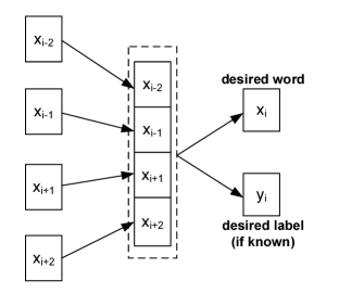
Figure 1: An Illustration of the Semi-supervised Word Embedding Model.

4.1.2 The Training Algorithm

The training algorithm used in the Word2Vec model first learns how to update the weights on the network edges assuming the word vectors are given (randomly initialized); then it learns how to update the word vectors assuming the weights on the edges are given (randomly initialized). It repeats these two steps until all the words in the input corpus have been processed.

We produce a “true label” vector, and add it as an extra set of output nodes to the neural network. This vector has 148 entries corresponding to 133 medical semantic types and 15 semantic groups. If a term is associated with some semantic types and semantic groups, the corresponding entries will be set to 1, otherwise 0. Increasing the size of the output layer will slow down the computation. For example, compared to the original Word2Vec “Negative Sampling” strategy with 150 negative samples, the semi-supervised method will be about $50\%$ slower.

This section derives new update rules for word vectors and edge weights. Since the semi-supervised approach is an extension of the original Word2vec model, the derivation is also similar. The new update rules work for all 4 Word2Vec settings mentioned in Section 2. The notations used in this section are defined in Figure 2.

$\delta(x)=1/(1+e^{-x})$; $V$ is a vocabulary set with $|V|$ distinct words; $W=\{w_{1}\cdots w_{|V|}\}$ is the set of embeddings for all the words in $V$; $w_{k}$ is the embedding for word $k$ in $V$; $\theta_{k}$ is a mapping function associated with word $k$; $X=\{x_{1},\cdots x_{N}\}$ represents all the words in a corpus $\mathcal{X}$; $x_{i}$ is the $i^{th}$ word in $X$; $c_{i}=[w_{c_{i}^{1}},\cdots w_{c_{i}^{l}}]$ represents the embeddings of all $l$ context words for word $x_{i}$ in $X$; $L$ is a label set with $|L|$ distinct labels; $X_{U}$ represents all the words without known labels in $X$; $X_{L}$ represents all the words with known labels in $X$; $X=\{X_{L},X_{U}\}$; $Y_{i}\in L$ is a set of known labels associated with $x_{i}$; Note that $x_{i}$ may have multiple labels; $Y_{i}=\{\}$, when $x_{i}$’s label is unknown; $\eta$ is the learning rate;

Figure 2: Notations

It can be verified that the following formulas will always hold:

$$\partial(\delta(x))/\partial x=\delta(x)\cdot(1-\delta(x))$$

$$\partial(\log\delta(x))/\partial x=1-\delta(x)$$

$$\partial(\log(1-\delta(x)))/\partial x=-\delta(x)$$

$\pi_{S}(x)$ is defined as

$$\pi_{S}(x)=\left\{\begin{array}[]{c}1,\,\,\,x\in S;\\ 0,\,\,\,otherwise;\\ \end{array}\right.$$

Given a word $x_{i}$, we first compute the context vector $c_{i}$ by concatenating the embeddings of all the contextual words of $x_{i}$. Then we simultaneously maximize the probability to predict its “desired word” and the “true label” (if known).

$$f(u|c_{i})=\left\{\begin{array}[]{c}\delta(\theta_{u}^{\prime}c_{i}),\pi_{\{x_{i},Y_{i}\}}(u)=1\\ 1-\delta(\theta_{u}^{\prime}c_{i}),\pi_{\{x_{i},Y_{i}\}}(u)=0\\ \end{array}\right.$$

$f(u|c_{i})$ can also be written as

$$f(u|c_{i})=\delta(\theta_{u}^{\prime}c_{i})^{\pi_{\{x_{i},Y_{i}\}}(u)}\cdot(1-\delta(\theta_{u}^{\prime}c_{i}))^{1-\pi_{\{x_{i},Y_{i}\}}(u)}$$

To make the explanation simpler, we define $F(x_{i},u)$, $F(x_{i})$ and $F$ as follows:

$$F(x_{i},u)=f(u|c_{i}),\,\,\,F(x_{i})=\prod_{u\in V}f(u|c_{i}),\,\,\,F=\prod_{x_{i}\in X}F(x_{i})$$

To achieve our goal, we want to maximize $F$ for the given $X$:

$$F=\prod_{x_{i}\in X}\prod_{u\in V}f(u|c_{i})$$

Apply $\log$ to both sides of the above equation, we have

$$\log F = \sum_{x_{i}\in X}\sum_{u\in V}\log f(u|c_{i})$$

$$= \sum_{x_{i}\in X}\sum_{u\in V}\log[\delta(\theta_{u}^{\prime}c_{i})^{\pi_{\{x_{i},Y_{i}\}}(u)}$$

$$\cdot (1-\delta(\theta_{u}^{\prime}c_{i}))^{1-\pi_{\{x_{i},Y_{i}\}}(u)}]$$

$$= \sum_{x_{i}\in X}\sum_{u\in V}\pi_{\{x_{i},Y_{i}\}}(u)\cdot\log\delta(\theta_{u}^{\prime}c_{i})$$

$$+ (1-\pi_{\{x_{i},Y_{i}\}}(u))\cdot\log(1-\delta(\theta_{u}^{\prime}c_{i}))$$

Now we compute the first derivative of $\log F(x_{i},u)$ on both $\theta_{u}$ and $c_{i}$:
$\partial\log F(x_{i},u)/\partial\theta_{u}$

$$= \pi_{\{x_{i},Y_{i}\}}(u)\cdot(1-\delta(\theta_{u}^{\prime}c_{i}))\cdot c_{i}$$

$$- (1-\pi_{\{x_{i},Y_{i}\}}(u))\cdot\delta(\theta_{u}^{\prime}c_{i})\cdot c_{i}$$

$$= (\pi_{\{x_{i},Y_{i}\}}(u)-\delta(\theta_{u}^{\prime}c_{i}))\cdot c_{i}$$

$\partial\log F(x_{i},u)/\partial c_{i}$

$$=(\pi_{\{x_{i},Y_{i}\}}(u)-\delta(\theta_{u}^{\prime}c_{i}))\cdot\theta_{u}$$

The new update rules to update $\theta_{u}$ (weights on the edges) and $c_{i}$ (word vectors) are as follows:

$$\theta_{u} = \theta_{u}+\eta\cdot(\pi_{\{x_{i},Y_{i}\}}(u)-\delta(\theta_{u}^{\prime}c_{i}))\cdot c_{i}$$ (3)

$$c_{i} = c_{i}+\eta\cdot(\pi_{\{x_{i},Y_{i}\}}(u)-\delta(\theta_{u}^{\prime}c_{i}))\cdot\theta_{u}$$ (4)

4.2 Expansion of the Raw Features

The semi-supervised term embedding model returns us with the vector representation for each term. To capture more information useful for synonym extraction, we expand the raw features with several heuristic rule-based matching features and several other simple feature expansions. All these expanded features together with the raw features form a concept space for synonym extraction.

Notations used in this section are summarized here: for any pair of the input terms: $a$ and $b$, we represent their lengths (number of words) as $|a|$ and $|b|$. $a$ and $b$ can be multi-word terms (like “United States”) or single-word terms (like “student”). We represent the raw feature vector of $a$ as $A$, and the raw feature vector of $b$ as $B$.

4.2.1 Rule-based Matching Features

The raw features can only help model the distributional similarity of two terms based on the corpus and the existing medical knowledge. In this section, we provide several matching features to model the similarity of two terms based on the surface form. These rule-based matching features $m_{1}$ to $m_{6}$ are generated as follows:

• $m_{1}$: returns the number of the common words shared by $a$ and $b$.

• $m_{2}$: $m_{1}/(|a|\cdot|b|)$;

• $m_{3}$: if $a$ and $b$ only differ by an antonym prefix, returns 1; otherwise, 0. The antonym prefix list includes character sequences like “anti”, “dis”, “il”, “im”, “in”, “ir” “non” and “un”, et al. For example, $m_{3}=1$ for “like” and “dislike”.

• $m_{4}$: if all the upper case characters from $a$ and $b$ match each other, returns 1; otherwise, 0. For example, $m_{4}=1$ for “USA” and ”United States of America”.

• $m_{5}$: if all the first characters in each word from $a$ and $b$ match each other, returns 1; otherwise, 0. For example, $m_{5}=1$ for “hs” and “hierarchical softmax”.

• $m_{6}$: if one term is the subsequence of another term, returns 1; otherwise, 0.

4.2.2 Feature Expansions

In addition to the matching features, we also produce several other straightforward expansions, including

• “sum”: $[A+B]$

• “difference”: $[\,|A-B|\,]$

• “product”: $[A\cdot B]$

• $[m_{2}\cdot A\,\,,\,\,m_{2}\cdot B]$

5 Experiments

In our experiments, we used the MedicalESG parser McCord et al. (2012) to parse all 130M sentences in the corpus, and extracted all the terms from the sentences. For those terms that are associated with CUIs, we assigned each of them with a set of semantic types/groups through a CUI lookup in UMLS.

Section 5.1 presents how the training and test sets were created. Section 5.2 is about the baseline approaches used in our experiments. In Section 5.3, we compare the new models and the baseline approaches on medical synonym extraction task. To measure the scalability, we also used our best synonym extractor to build a new medical synonym knowledgebase. Then we analyze the contribution of each individual feature to the final results in Section 5.4.

5.1 Data Collection

UMLS has about 300K CUI pairs under the relations (see Table 1) corresponding to synonyms. However, the majority of them contain the CUIs that are not in our corpus. The goal of this paper is to detect new synonyms from text, so only the relation instances with both CUIs in the corpus are used in the experiments. A CUI starts with letter ‘C’, and is followed by 7 digits. We use the preferred name, which is a term, as the surface form for each CUI. Our preprocessing step resulted in a set of 8,000 positive synonym examples. To resemble the real-world challenges, where most of the given term pairs are non-synonyms, we randomly generated more than 1.6M term pairs as the negative examples. For these negative examples, both terms are required to occur at least twice in our corpus. Some negative examples generated in this way may be in fact positives, but this should be very rare.

The final dataset was split into 3 parts: 60% examples were used for training, 20% were used for testing the classifiers, and the remaining 20% were held out to evaluate the knowledgebase construction results.

5.2 Baseline Approaches

Both the LSA model Deerwester et al. (1990) and the Word2Vec model Mikolov et al. (2013) were built on our medical corpus as discussed in Section 3.1, which has about 130M sentences and 15M unique terms. We constructed Word2Vec as well as the semi-supervised term embedding models under all 4 different settings: HS+CBOW, HS+SkipGram, NEG+CBOW, and NEG+SkipGram. The parameters used in the experiments were: dimension_size=100, window_size=5, negative=10, and sample_rate=1e-5. We obtained 100 dimensional embeddings from all these models. Word2Vec models typically took a couple of hours to train, while LSA model required a whole day training on a computer with 16 cores and 128G memory. The feature expansion (Section 4.2) was applied to all these baseline approaches as well.

The letter $n$-gram model Huang et al. (2013) used in our experiments was slightly different from the original one. We added special letter $n$-grams on top of the original one to model the begin and end of each term. In our letter $n$-gram experiments, we tested $n=2,3$ and $4$. The letter $n$-gram model does not require training.

5.3 Synonym Extraction Results

The focus of this paper is to find a good concept space for synonym extraction, so we prefer a simple classifier over a complicated one in order to more directly measure the impact of the features (in the concept space) on the performance. The speed is one of our major concerns, and we have about 1M training examples to process, so we used the liblinear package Fan et al. (2008) in our experiments for its high speed and good scalability. In all the experiments, the weight for the positive examples was set to 100, due to the fact that most of the input examples were negative. All the other parameters were set to the default values. The evaluation of different approaches is based on the $F_{1}$ scores, and the final results are summarized in Table 3.

Table 3: $F_{1}$ Scores of All Approaches on both the Training and the Test Data.

Approach	Training $F_{1}$	Test $F_{1}$
LSA	48.98%	48.13%
Letter-BiGram	55.51%	50.09%
Letter-TriGram	96.30%	63.37%
Letter-FourGram	99.48%	66.50%
Word2Vec HS+CBOW	64.05%	63.51%
Word2Vec HS+SKIP	64.23%	62.65%
Word2Vec NEG+CBOW	59.47%	58.75%
Word2Vec NEG+SKIP	70.17%	67.86%
Concept Space HS+CBOW	68.15%	65.73%
Concept Space HS+SKIP	74.25%	70.74%
Concept Space NEG+CBOW	63.57%	60.90%
Concept Space NEG+SKIP	74.09%	70.97%

From the results in Table 3, we can see that the LSA model returns the lowest $F_{1}$ score of $48.13\%$, followed by the letter bigram model ($50.09\%$). The letter trigram and 4-gram models return very competitive scores as high as $66.50\%$, and it looks like increasing the value of $n$ in the letter-$n$gram model will push the $F_{1}$ score up even further. However, we have to stop at $n=4$ for two reasons. Firstly, when $n$ is larger, the model is more likely to overfit for the training data, and the $F_{1}$ score for the letter 4-gram model on the training data is already $99.48\%$. Secondly, the resulting model will be more complicated for $n>4$. For the letter 4-gram model, the model file itself is already about 3G big on the disk, making it very expensive to use.

The best setting of the Word2Vec model returns a $67.86\%$ $F_{1}$ score. This is about $3\%$ lower than the best setting of the concept space model, which achieves the best $F_{1}$ score across all approaches: $70.97\%$. We also compare the Word2Vec model and the concept space model under all 4 different settings in Table 4. The concept space model outperforms the original Word2Vec model by a large margin ($3.9\%$ on average) under all of them.

Since we have a lot of training data, and are using a linear model as the classifier, the training part is very stable. We ran a couple of other experiments (not reported in this paper) by expanding the training set and the test set with the dataset held out for knowledgebase evaluation, but did not see too much difference in terms of the $F_{1}$ scores.

Table 4: $F_{1}$ Scores of the Word2Vec and the Concept Space Models on the Test Data.

Setting	Wored2Vec	Concept Space	Diff
HS+CBOW	63.51%	65.73%	+2.22%
HS+SKIP	62.65%	70.74%	+8.09%
NEG+CBOW	58.75%	60.90%	+2.15%
NEG+SKIP	67.86%	70.97%	+3.11%
Average	63.19%	67.09%	+3.90%

Table 5: Analysis of the Feature Contributions to $F_{1}$ for the Concept Space Model.

$F_{1}$	HS+	HS+	NEG+	NEG+	Average	Average
	CBOW	SKIP	CBOW	SKIP	Score	Improvement
$[A,B]$	44.28%	51.19%	41.42%	53.37%	47.57%	-
+ [matching features]	57.81%	63.53%	54.63%	62.37%	59.59%	+12.02%
+ $[A+B]$ and $[|A-B|]$	62.71%	70.37%	61.04%	69.02%	65.79%	+6.20%
+ $[A\cdot B]$	66.20%	68.61%	60.40%	70.18%	66.35%	+0.56%
+ $[m_{2}\cdot[A,B]]$	65.73%	70.74%	60.90%	70.97%	67.09%	+0.74%

Our method was very scalable. It took on average several hours to generate the word embedding file from our medical corpus with 20G text using $16\times 3.2$G cpus and roughly 30 minutes to finish the training process using one cpu. To measure the scalability at the apply time, we constructed a new medical synonym knowledgebase with our best synonym extractor. This was done by applying the concept space model trained under the NEG+SKIP setting to a set of 11B pairs of terms. All these terms are associated with CUIs, and occur at least twice in our medical corpus. This KB construction process finished in less than 10 hours using one cpu, resulting in more than 3M medical synonym term pairs. To evaluate the recall of this knowledgebase, we checked each term pair in the held out synonym dataset against this KB, and found that more than $42\%$ of them were covered by this new KB. Precision evaluation of this KB requires a lot of manual annotation effort, and will be included in our future work.

5.4 Feature Contribution Analysis

In Section 4.2, we expand the raw features with the matching features and several other feature expansions to model the term relationships. In this section, we study the contribution of each individual feature to the final results. We added all those expanded features to the raw features one by one and re-ran the experiments for the concept space model. The results and the feature contributions are summarized in Table 5.

The results show that adding matching features, “sum” and “difference” features can significantly improve the $F_{1}$ scores. We can also see that adding the last two feature sets does not seem to contribute a lot to the average $F_{1}$ score. However, they do contribute significantly to our best $F_{1}$ score by about $2\%$ .

6 Conclusions

In this paper, we present an approach to construct a medical concept space from manually extracted medical knowledge and a large corpus with 20G unstructured text. Our approach extends the Word2Vec model by making use of the medical knowledge as extra label information during the training process. This new approach fits well for the medical domain, where the language use variability is exceptionally high and the existing knowledge is also abundant.

Experiment results show that the proposed model outperforms the baseline approaches by a large margin on a dataset with more than one million term pairs. Future work includes doing a precision analysis of the resulting synonym knowledgebase, and exploring how deep learning models can be combined with our concept space model for better synonym extraction.

References

- Barzilay and Elhadad (1999) R. Barzilay and M. Elhadad. Using lexical chains for text summarization. In I. Mani and M. T. Maybury, editors, Advances in Automatic Text Summarization. The MIT Press, 1999.
- Bengio et al. (2003) Y. Bengio, R. Ducharme, P. Vincent, and C. Janvin. A neural probabilistic language model. Journal of Machine Learning Research, 3, 2003.
- Blondel et al. (2004) V. D. Blondel, A. Gajardo, M. Heymans, P. Senellart, and P. V. Dooren. A measure of similarity between graph vertices: applications to synonym extraction and web searching. SIAM Review, 46(4), 2004.
- Brown et al. (1992) P. F. Brown, P. V. deSouza, R. L. Mercer, V. J. Della Pietra, and J. C. Lai. Class-based n-gram models of natural language. Compututational Linguistics, 18(4), 1992.
- Collobert and Weston (2008) R. Collobert and J. Weston. A unified architecture for natural language processing: Deep neural networks with multitask learning. In Proceedings of the 25th International Conference on Machine Learning, 2008.
- Curran (2002) J. R. Curran. Ensemble methods for automatic thesaurus extraction. In Proceedings of the Conference on Empirical Methods in Natural Language Processing (EMNLP), 2002.
- Curran (2008) J. R. Curran. Learning graph walk based similarity measures for parsed text. In Proceedings of the Conference on Empirical Methods in Natural Language Processing (EMNLP), 2008.
- Deerwester et al. (1990) S. Deerwester, S. T. Dumais, G. W. Furnas, T. K. Landauer, and R. Harshman. Indexing by latent semantic analysis. Journal of the American Society for Information Science, 41(6):391–407, 1990.
- Dumais and Landauer (1997) S. Dumais and T. Landauer. A solution to platos problem: the latent semantic analysis theory of acquisition, induction and representation of knowledge. Psychological Review, 104(2), 1997.
- Fan et al. (2008) R. E. Fan, K. W. Chang, C. J. Hsieh, X. R. Wang, and C. J. Lin. Liblinear: A library for large linear classification. Journal of Machine Learning Research, 9:1871–1874, 2008.
- Ferrucci (2012) D. Ferrucci. Introduction to “This is Watson”. IBM Journal of Research and Development, 56, 2012.
- Glorot et al. (2011) X. Glorot, A. Bordes, and Y. Bengio. Domain adaptation for large-scale sentiment classification: A deep learning approach. In Proceedings of the 28th International Conference on Machine Learning, 2011.
- Hearst (1992) M. Hearst. Automatic acquisition of hyponyms from large text corpora. In Proceedings of the International Conference on Computational Linguistics (COLING), 1992.
- Henriksson et al. (2013a) A. Henriksson, M. Conway, M. Duneld, and W. W. Chapman. Identifying synonymy between SNOMED clinical terms of varying length using distributional analysis of electronic health records. In Proceedings of AMIA Annual Symposium., 2013.
- Henriksson et al. (2013b) A. Henriksson, M. Skeppstedt, M. Kvist, M. Conway, and M. Duneld. Corpus-driven terminology development: populating Swedish SNOMED CT with synonyms extracted from electronic health records. In Proceedings of BioNLP, 2013.
- Henriksson et al. (2014) A. Henriksson, H. Moen, M. Skeppstedt, V. Daudaravicius, and M. Duneld. Synonym extraction and abbreviation expansion with ensembles of semantic spaces. Journal of Biomedical Semantics, 5(6), 2014.
- Huang et al. (2013) P. Huang, X. He, J. Gao, L. Deng, A. Acero, and L. Heck. Learning deep structured semantic models for web search using clickthrough data. In Proceedings of the ACM International Conference on Information and Knowledge Management (CIKM), 2013.
- Lebret and Collobert (2014) R. Lebret and R. Collobert. Word embeddings through Hellinger PCA. In Proceedings of the 14th Conference of the European Chapter of the Association for Computational Linguistics, 2014.
- Lindberg et al. (1993) D. Lindberg, B. Humphreys, and A. McCray. The Unified Medical Language System. Methods of Information in Medicine, 32:281–291, 1993.
- McCord et al. (2012) M. McCord, J. W. Murdock, and B. K. Boguraev. Deep parsing in Watson. IBM Journal of Research and Development, 56, 2012.
- Meystre et al. (2008) S. M. Meystre, G. K. Savova, K. C. Kipper-Schuler, and J. F. Hurdle. Extracting information from textual documents in the electronic health record: a review of recent research. Yearbook of Medical Informatics, 47(1), 2008.
- Mikolov et al. (2013) T. Mikolov, K. Chen, G. Corrado, and J. Dean. Efficient estimation of word representations in vector space. In Proceedings of the Workshop at International Conference on Learning Representations, 2013.
- Mnih and Teh (2012) A. Mnih and Y. W. Teh. A fast and simple algorithm for training neural probabilistic language models. In Proceedings of the 29th International Conference on Machine Learning (ICML), 2012.
- Nakayama et al. (2007) K. Nakayama, T. Hara, and S. Nishio. Wikipedia mining for an association web thesaurus construction. In Proceedings of the International Conference on Web Information Systems Engineering, 2007.
- Passos et al. (2014) A. Passos, V. Kumar, and A. McCallum. Lexicon infused phrase embeddings for named entity resolution. In Proceedings of the 18th Conference on Computational Language Learning, 2014.
- Peirsman and Geeraerts (2009) Y. Peirsman and D. Geeraerts. Predicting strong associations on the basis of corpus data. In Proceedings of the 12th Conference of the European Chapter of the Association for Computational Linguistics, 2009.
- Pennington et al. (2014) J. Pennington, R. Socher, and C. D. Manning. Glove: Global vectors for word representation. In Proceedings of the Conference on Empirical Methods in Natural Language Processing (EMNLP), 2014.
- Rumelhart et al. (1986) D. E. Rumelhart, G. E. Hinton, and R. J. Williams. Parallel distributed processing: Explorations in the microstructure of cognition, vol. 1. pages 318–362. MIT Press, 1986.
- Saeed (2009) J. I. Saeed. Semantics. Wiley-Blackwell, 3rd edition, 2009.
- Socher et al. (2011) R. Socher, C. C. Lin, A. Ng, and C. D. Manning. Parsing natural scenes and natural language with recursive neural networks. In Proceedings of the 28th International Conference on Machine Learning (ICML), 2011.
- Turney and Pantel (2010) Peter D. Turney and Patrick Pantel. From frequency to meaning: Vector space models of semantics. Journal of Artificial Intelligence Research, 37(1):141–188, 2010.
- Wang and Hirst (2009) T. Wang and G. Hirst. Extracting synonyms from dictionary definitions. In Proceedings of International Conference of RANLP, 2009.
- Wu and Zhou (2003) H. Wu and M. Zhou. Optimizing synonym extraction using monolingual and bilingual resources. In Proceedings of the Second International Workshop on Paraphrasing, 2003.
- Zeng et al. (2012) Q. T. Zeng, D. Redd, T. Rindflesch, and J. Nebeker. Synonym, topic model and predicate-based query expansion for retrieving clinical documents. In Proceedings of AMIA Annual Symposium, 2012.