Hypergeometric polynomials are optimal

Abstract.

With any integer convex polytope $P\subset\hbox{\midBbb R}^{n}$ we associate a multivariate hypergeometric polynomial whose set of exponents is $\hbox{\midBbb Z}^{n}\cap P.$ This polynomial is defined uniquely up to a constant multiple and satisfies a holonomic system of partial differential equations of Horn’s type. We prove that under certain nondegeneracy conditions the zero locus of any such polynomial is optimal in the sense of [7], i.e., that the topology of its amoeba [11] is as complex as it could possibly be. Using this, we derive optimal properties of several classical families of multivariate hypergeometric polynomials.

1. Introduction

Zeros of hypergeometric functions are known to exhibit highly complicated behavior. The univariate case has been extensively studied both classically (see e.g. [10, 12]) and recently (see [3, 4, 21] and the references therein). Already the distribution of zeros of polynomial instances of the simplest non-elementary hypergeometric function ${}_{2}F_{1}\left(a,b;c;x\right)$ is far from being clear. By letting the parameters $a,b,c$ assume values in various ranges, one can obtain a wide variety of shapes. Some of them are highly regular (see e.g. Fig. 1) while other are nearly chaotic.

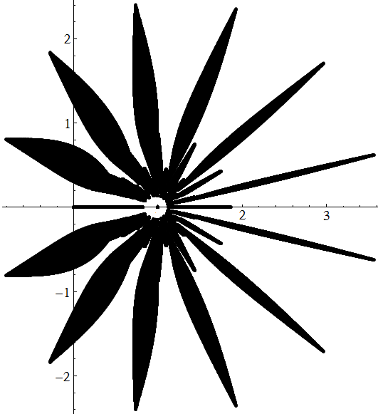
Figure 1. The hypergeometric aster: zeros of the polynomials ${}_{2}F_{1}\left(-12,b;c;x\right)$ with $b,c\in\left\{\frac{k}{1000}:k=100,\ldots,4000\right\}$

Polynomial instances of hypergeometric functions in one and several variables are very diverse. They comprise the classical Chebyshev polynomials of the first and the second kind, the Gegenbauer, Hermite, Jacobi, Laguerre and Legendre polynomials as well as their numerous multivariate analogues [5].

Despite the diversity of families of hypergeometric polynomials, most of them share the following key properties that justify the usage of the term ”hypergeometric”:

1. The polynomials are dense (possibly after a suitable monomial change of variables).

2. The coefficients of a hypergeometric polynomial are related through some recursion with polynomial coefficients.

3. For univariate polynomials, there is typically a single representative (up to a suitable normalization) of a given degree within a family of hypergeometric polynomials.

4. All polynomials in the family satisfy a differential equation of a fixed order with polynomial coefficients (or a system of such equations) whose parameters encode the degree of a polynomial.

5. In the case of one dimension, the absolute values of the roots of a classical hypergeometric polynomial are all different (possibly after a suitable monomial change of variables).

6. Many of hypergeometric polynomials enjoy various extremal properties.

In the present paper, we introduce a definition of a multivariate hypergeometric polynomial in $n\geq 2$ complex variables that is coherent with the properties 1-6 listed above. Namely, with any integer convex polytope $P\subset\hbox{\Bbb R}^{n}$ we associate a multivariate hypergeometric polynomial whose set of exponents is $\hbox{\Bbb Z}^{n}\cap P.$ For this polynomial to be truly hypergeometric in the sense made precise below, we need to assume that any pair of points in $\hbox{\Bbb Z}^{n}\cap P$ can be connected by a polygonal line with unit sides and integer vertices. This assumption does not affect the generality of the results since any polytope that does not satisfy this condition gives rise to a finite number of hypergeometric polynomials that can be considered independently. The assumption of convexity of the polytope $P$ is then automatically satisfied as clarified in Lemma 3.4.

The hypergeometric polynomial associated with the polytope $P$ is defined uniquely up to a constant multiple and satisfies a holonomic system of partial differential equations of Horn’s type [16, 18]. We prove that under certain nondegeneracy conditions (see Theorem 3.10) the zero locus of any such polynomial is optimal in the sense of [7]. Generally speaking, this means that the topology of the amoeba [7, 11] of such a polynomial is as complicated as it could possibly be (see Definition 2.8). This property is the multivariate counterpart of the property of having different absolute values of the roots for a polynomial in a single variable. We show various families of classically known multivariate polynomials to be optimal: a biorthogonal basis in the unit ball, certain polynomial instances of the Appel $F_{1}$ function, bivariate Chebyshev polynomials of the second kind etc. We also introduce a simplicial complex that encodes intrinsic combinatorial properties of an algebraic variety while possessing key properties of its compactified amoeba.

Pictures of amoebas in the paper have been created with Matlab 7.9. The authors are thankful to L. Lang for valuable comments on the paper.

2. Hypergeometric systems and amoebas

Throughout the paper, we denote by $n$ the number of $x\in\hbox{\Bbb C}^{n}$ variables. For $\alpha=(\alpha_{1},\ldots,\alpha_{n}),$ we use the notation $|\alpha|=\sum_{i=1}^{n}\alpha_{i}$ and $\alpha!=\alpha_{1}!\ldots\alpha_{n}!.$ For $x=(x_{1},\ldots,x_{n})$ and $\alpha=(\alpha_{1},\ldots,\alpha_{n}),$ we denote by $x^{\alpha}$ the monomial $x_{1}^{\alpha_{1}}\ldots x_{n}^{\alpha_{n}}.$

Definition 2.1.

A formal Laurent series

(2.1) $$\sum_{s\in\hbox{\midBbb Z}^{n}}\varphi(s)\,x^{s}$$

is called hypergeometric if for any $j=1,\ldots,n$ the quotient $\varphi(s+e_{j})/\varphi(s)$ is a rational function in $s=(s_{1},\ldots,s_{n}).$ Throughout the paper we denote this rational function by $P_{j}(s)/Q_{j}(s+e_{j}).$ Here ${\{e_{j}\}}_{j=1}^{n}$ is the standard basis of the lattice $\hbox{\Bbb Z}^{n}.$ By the support of this series we mean the subset of $\hbox{\Bbb Z}^{n}$ on which $\varphi(s)\neq 0.$

By a hypergeometric function we will mean a (typically multi-valued) analytic function obtained by means of analytic continuation of a hypergeometric series with a nonempty domain of convergence along all possible paths in $\hbox{\Bbb C}^{n}$.

Theorem 2.2.

(Ore, Sato, see [8].) The coefficients of a hypergeometric series are given by the formula

(2.2) $$\varphi(s)=t^{s}\,U(s)\,\prod_{i=1}^{m}\Gamma(\langle{\bf A}_{i},s\rangle+c_{i}),$$

where $t^{s}=t_{1}^{s_{1}}\ldots t_{n}^{s_{n}},$ $t_{i},c_{i}\in\hbox{\Bbb C},$ ${\bf A}_{i}=(A_{i,1},\ldots,A_{i,n})$ $\in\hbox{\Bbb Z}^{n},$ $i=1,\ldots,m,$ and $U(s)$ is the product of a certain rational function and a periodic function $\phi(s)$ such that $\phi(s+e_{j})\equiv\phi(s)$ for every $j=1,\ldots,n$.

Given the above data ($t_{i},c_{i},{\bf A}_{i},U(s)$) that determines the coefficient of a hypergeometric series, it is straightforward to compute the rational functions $P_{i}(s)/Q_{i}(s+e_{i})$ using the $\Gamma$-function identity. The converse requires solving a system of difference equations which is only solvable under some compatibility conditions on $P_{i},Q_{i}.$ A careful analysis of this system of difference equations has been performed in [16].

We will call any function of the form (2.2) the Ore-Sato coefficient of a hypergeometric series. In this paper the Ore-Sato coefficient (2.2) plays the role of a primary object which generates everything else: the series, the hypergeometric system of differential equations, its polynomial solution (if any) and its amoeba. We will also assume that $m\geq n$ since otherwise the corresponding hypergeometric series (2.1) is just a linear combination of hypergeometric series in fewer variables (times an arbitrary function in remaining variables that makes the system non-holonomic) and $n$ can be reduced to meet the inequality.

Definition 2.3.

The Horn system of an Ore-Sato coefficient. A (formal) Laurent series $\sum_{s\in\hbox{\midBbb Z}^{n}}\varphi(s)x^{s}$ whose coefficient satisfies the relations $\varphi(s+e_{j})/\varphi(s)=P_{j}(s)/Q_{j}(s+e_{j})$ is a (formal) solution to the following system of partial differential equations of hypergeometric type

(2.3) $$x_{j}P_{j}(\theta)f(x)=Q_{j}(\theta)f(x),\,\,\,j=1,\ldots,n.$$

Here $\theta=(\theta_{1},\ldots,\theta_{n}),$ $\theta_{j}=x_{j}\frac{\partial}{\partial x_{j}}.$ The system (2.3) will be referred to as the Horn hypergeometric system defined by the Ore-Sato coefficient $\varphi(s)$ (see [8]) and denoted by ${\rm Horn}(\varphi)$. In this paper we only treat holonomic Horn hypergeometric systems, i.e. ${\rm rank}({\rm Horn}(\varphi))$ is always assumed to be finite.

We will often be dealing with the important special case of an Ore-Sato coefficient (2.2) where $t_{i}=1$ for any $i=1,\ldots,n$ and $U(s)\equiv 1.$ The Horn system associated with such an Ore-Sato coefficient will be denoted by ${\rm Horn}(A,c),$ where $A$ is the matrix with the rows ${\bf A}_{1},\ldots,{\bf A}_{m}\in\hbox{\Bbb Z}^{n}$ and $c=(c_{1},\ldots,c_{m})\in\hbox{\Bbb C}^{m}.$ In this case the following operators $P_{j}(\theta)$ and $Q_{j}(\theta)$ explicitly determine the system (2.3):

$$P_{j}(s)=\prod_{i:A_{i,j}>0}\prod_{\ell_{j}^{(i)}=0}^{A_{i,j}-1}\left(\langle{\bf A}_{i},s\rangle+c_{i}+\ell_{j}^{(i)}\right),\quad Q_{j}(s)=\prod_{i:A_{i,j}<0}\prod_{\ell_{j}^{(i)}=0}^{|A_{i,j}|-1}\left(\langle{\bf A}_{i},s\rangle+c_{i}+\ell_{j}^{(i)}\right).$$

Definition 2.4.

The support of a series solution to (2.3) is called irreducible if there exists no series solution to (2.3) supported in its proper nonempty subset.

Definition 2.5.

The amoeba $\mathcal{A}_{f}$ of a Laurent polynomial $f(x)$ (or of the algebraic hypersurface $\{f(x)=0\}$) is defined to be the image of the hypersurface $f^{-1}(0)$ under the map ${\rm Log}:(x_{1},\ldots,x_{n})\mapsto(\log|x_{1}|,\ldots,\log|x_{n}|).$

Despite losing $n$ real dimensions, the amoeba of an algebraic hypersurface encodes its several intrinsic properties [7, 14, 19]. The main results of the paper describe topological properties of the amoebas of hypergeometric polynomials. The next lemma shows that certain transformations of a polynomial do not affect the topology of its amoeba.

Lemma 2.6.

The number of connected components of the amoeba complement of a (Laurent) polynomial $p(x_{1},\ldots,x_{n})$ is the same as that of the polynomial $x^{a}p(t_{1}x^{v_{1}},\ldots,t_{n}x^{v_{n}})^{\ell}$ for any $\ell\in\hbox{\Bbb N},$ $a=(a_{1},\ldots,a_{n})\in\hbox{\Bbb Z}^{n},$ $t=(t_{1},\ldots,t_{n})\in(\hbox{\Bbb C}^{*})^{n}$ and any nondegenerate integer matrix $v$ with the rows $v_{1},\ldots,v_{n}.$ That is, there is a bijection between the connected components of the complements of the two amoebas; moreover, the orders [7] and the recession cones [13] of the corresponding components are transformed into each other by the linear map with the matrix $v$.

Proof.

A monomial factor can only vanish in the union of the coordinate hyperplanes that is mapped off to infinity by the logarithmic map. The amoeba does not reflect the multiplicities of the zeros of a polynomial and it can therefore be raised to any positive power. The map $(x_{1},\ldots,x_{n})\mapsto(t_{1}x_{1},\ldots,t_{n}x_{n})$ corresponds to the shift of the amoeba space with respect to the vector $\log|t_{1}|,\ldots,\log|t_{n}|.$ Finally, a nondegenerate monomial change of variables in the complex torus $(\hbox{\Bbb C}^{*})^{n}$ corresponds to the linear transformation of the amoeba space defined by the matrix of exponents of the monomials. Clearly a nondegenerate linear map preserves the topology of amoebas and provides a bijection for the recession cones of the complement components. The last statement of the lemma is an immediate consequence of the definition of the order of a component in the amoeba complement [7]. ∎

Recall that the Newton polytope $\mathcal{N}_{p(x)}$ of a Laurent polynomial $p(x)$ is defined to be the convex hull in $\hbox{\Bbb R}^{n}$ of the support of $p(x).$ The following result shows that the Newton polytope $\mathcal{N}_{p(x)}$ reflects the structure of the amoeba $\mathcal{A}_{p(x)}$ [7, Theorem 2.8 and Proposition 2.6].

Theorem 2.7.

(See [7].) Let $p(x)$ be a Laurent polynomial and let $\{M\}$ denote the family of connected components of the amoeba complement ${}^{c}\!\mathcal{A}_{p(x)}.$ There exists an injective function $\nu:\{M\}\rightarrow\hbox{\Bbb Z}^{n}\cap\mathcal{N}_{p(x)}$ such that the cone which is dual to $\mathcal{N}_{p(x)}$ at the point $\nu(M)$ coincides with the recession cone [13] of $M.$ In particular, the number of connected components of ${}^{c}\!\mathcal{A}_{p(x)}$ cannot be smaller than the number of vertices of $\mathcal{N}_{p(x)}$ and cannot exceed the number of integer points in $\mathcal{N}_{p(x)}.$

The two extreme values for the number of connected components of the complement of an amoeba are of particular interest.

Definition 2.8.

(Cf. [7, Definition 2.9].) An algebraic hypersurface $\mathcal{H}\subset(\hbox{\Bbb C}^{*})^{n},$ $n\geq 2,$ is called optimal if the number of connected components of its amoeba complement ${}^{c}\!\mathcal{A}_{\mathcal{H}}$ equals the number of integer points in the Newton polytope of the defining polynomial of $\mathcal{H}.$ We will say that a polynomial (as well as its amoeba) is optimal if its zero locus is an optimal algebraic hypersurface.

Since the amoeba of a polynomial does not carry any information on the multiplicities of its roots, any one-dimensional amoeba (which is just a finite set of distinct points in $a_{1},\ldots,a_{k}\in\hbox{\Bbb R}$) can be treated as the amoeba of the polynomial $\prod\limits_{j=1}^{k}(x-e^{a_{k}})$ all of whose roots are positive and distinct. Thus Definition 2.8 is trivial in the univariate case. The correct extension of Definition 2.8 to one dimension is to say that all the roots of the polynomial in question have different absolute values.

Example 2.9.

In accordance with Definition 2.3 the Ore-Sato coefficient

$$\varphi(s,t)=\Gamma(-s-t+1)\Gamma(2s-t-2)\Gamma(-s+2t-2)$$

yields the polynomials

$$\begin{array}[]{l}P_{1}(s,t)=(2s-t-2)(2s-t-1),\quad\quad Q_{1}(s,t)=(s-2t+2)(s+t-1),\\ P_{2}(s,t)=(s-2t+1)(s-2t+2),\quad\quad Q_{2}(s,t)=-(2s-t-2)(s+t-1).\end{array}$$

The corresponding Horn hypergeometric system is given by the linear differential operators

(2.4) $$\left\{\begin{array}[]{l}x\,(2\theta_{x}-\theta_{y}-2)(2\theta_{x}-\theta_{y}-1)-(\theta_{x}-2\theta_{y}+2)(\theta_{x}+\theta_{y}-1),\\ y\,(\theta_{x}-2\theta_{y}+1)(\theta_{x}-2\theta_{y}+2)+(2\theta_{x}-\theta_{y}-2)(\theta_{x}+\theta_{y}-1).\end{array}\right.$$

It is straightforward to check that (2.4) is satisfied by the hypergeometric polynomial $p(x,y)=x+y+6xy+x^{2}y^{2}.$

The amoeba of $p(x,y)$ together with its compactified version [11] are depicted in Fig. 2. We remark that the actual shapes of the amoeba and the compactified amoeba of $p(x,y)$ (with respect to both directions of the amoeba tentacles and the complement of its compact version) are rather different from those given in [11].

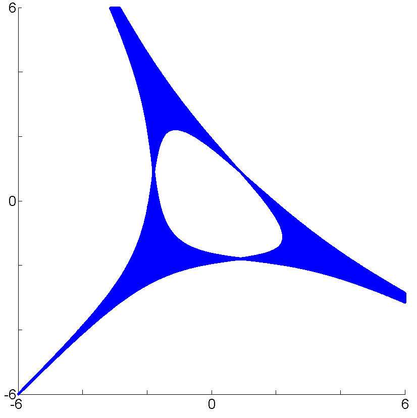
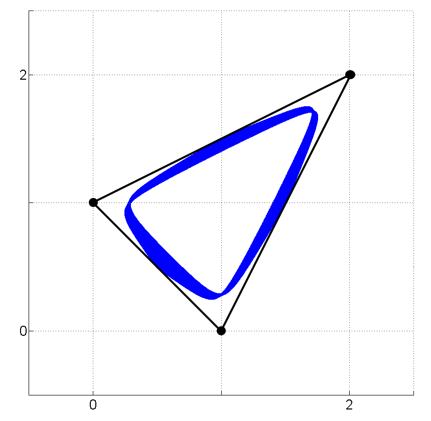
Figure 2. The amoeba and the compactified amoeba [11] of $p(x,y)$

An algebraic hypersurface is optimal if the topology of its amoeba is as complicated as it could possibly be in the view of Theorem 2.7 (that is, the number of connected components in the amoeba complement is maximal). A two-dimensional optimal amoeba has the maximal possible number of bounded connected components in its complement and the maximal number of parallel tentacles.

In the view of Lemma 2.6 we will not distinguish polynomials whose zero loci in $(\hbox{\Bbb C}^{*})^{n}$ can be transformed into each other by a nondegenerate monomial change of variables. The reason for this is illustrated by the following example.

Example 2.10.

A typical example of a family of optimal polynomials arising in a different theory is given by the biorthogonal family in the unit ball $\left\{V_{\alpha}(x)\right\}_{\alpha\in\hbox{\midBbb N}_{0}^{n}},$ $x\in\hbox{\Bbb C}^{n}$ defined through their generating function (see [5, Section 2.3]):

$$(1-2\langle a,x\rangle+\|a\|^{2})^{\frac{1-n}{2}}=\sum\limits_{\alpha\in\hbox{\midBbb N}_{0}^{n}}a^{\alpha}V_{\alpha}(x).$$

Neglecting an inessential monomial factor of $V_{\alpha}(x)$ (whose zero locus is contained in the union of the coordinate hyperplanes and therefore does not affect the amoeba, see Lemma 2.6) one can represent $V_{\alpha}(x)=\tilde{V}_{\alpha}(\xi)$ with $\tilde{V}_{\alpha}$ being a polynomial in $\xi_{j}=x_{j}^{2}.$ One can check that the zero locus of $\tilde{V}_{\alpha}(\xi)$ is an optimal algebraic hypersurface in $\hbox{\Bbb C}^{n}.$ The Newton polygon and the amoeba of the bivariate polynomial $\tilde{V}_{(6,10)}$ are depicted in Fig. 3.

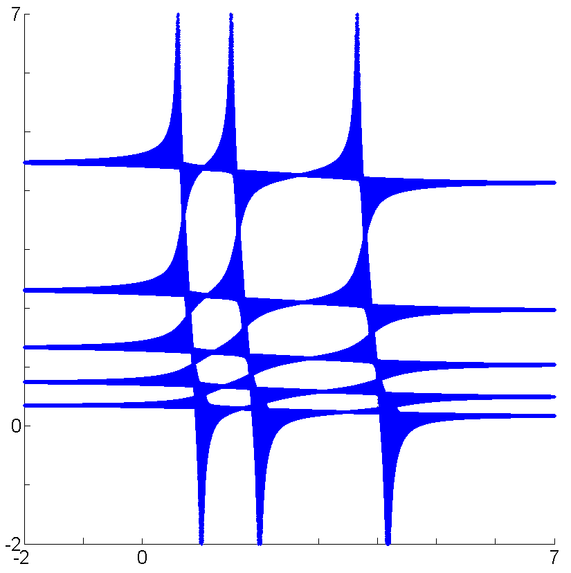
Figure 3. The Newton polygon of $\tilde{V}_{(6,10)}(x,y)$ in [5, Section 2.3] and its amoeba

Numerous other families of optimal multivariate polynomials can be found in [5, Chapter 2].

3. Hypergeometric polynomials in several variables

There exist several well-known and important families of hypergeometric polynomials [5, 21]. What they all have in common is the fact that they satisfy certain linear differential equations with polynomial coefficients that are special instances of (2.3). However, the family of all holonomic systems of partial differential equations of the form (2.3) is far too vast to serve as a definition of a hypergeometric polynomial. In fact, from the point of view of the general Definition 2.1 given above, any polynomial in any number of variables is a hypergeometric function. This is made precise in the following statement.

Theorem 3.1.

For any polynomial $p(x)\in\hbox{\Bbb C}[x_{1},\ldots,x_{n}]$ there exists a nonconfluent [13] holonomic hypergeometric system of the form (2.3) having $p(x)$ as one of its solutions. Moreover, it can be chosen in such a way that the hypergeometric ideal in the Weyl algebra defining this system admits a basis that consists of a commutative family of differential operators.

Proof.

In fact, any given polynomial is annihilated by a family of hypergeometric ideals that contains continuously many elements. To prove the theorem, we will present an explicit representative with desired properties.

Let $p(x)=\sum\limits_{\alpha\in S}c_{\alpha}x^{\alpha}$ be a polynomial with the support $S.$ Here and throughout the proof we assume $S$ to be finite. We denote by $\#S$ the cardinality of $S$ and let $|\alpha|=\alpha_{1}+\ldots+\alpha_{n}.$ For $s\in\hbox{\Bbb C}^{n}$ define the Ore-Sato coefficient $\varphi(s)$ by

(3.1) $$\varphi(s)=\frac{\prod\limits_{\alpha\in S}(s_{1}+\ldots+s_{n}-|\alpha|)}{\prod\limits_{j=1}^{n}\prod\limits_{\alpha\in S}(s_{j}-\alpha_{j})}.$$

By Definition 2.3, the action of the $j$-th hypergeometric differential operator in the system defined by this Ore-Sato coefficient on $p(x)$ is given by

$$\left(x_{j}\prod\limits_{\alpha\in S}(\theta_{1}+\ldots+\theta_{n}-|\alpha|)-\prod\limits_{\alpha\in S}(\theta_{j}-\alpha_{j})\right)\sum\limits_{\beta\in S}c_{\beta}x^{\beta}=$$

$$\sum\limits_{\beta\in S}c_{\beta}\left(\left(x_{j}\prod\limits_{\alpha\in S}(\theta_{1}+\ldots+\theta_{n}-|\alpha|)\right)x^{\beta}-\left(\prod\limits_{\alpha\in S}(\theta_{j}-\alpha_{j})\right)x^{\beta}\right)\equiv 0$$

since $\hbox{\Bbb C}[\theta_{1},\ldots,\theta_{n}]$ is a commutative subring in the Weyl algebra and $(\theta_{1}+\ldots+\theta_{n}-|\alpha|)x^{\alpha}=(\theta_{j}-\alpha_{j})x^{\alpha}\equiv 0$ for any $j=1,\ldots,n.$

The hypergeometric system defined by the Ore-Sato coefficient (3.1) is nonconfluent by definition. By Theorem 2.8 in [17] this system is holonomic with the holonomic rank $(\#S)^{n}.$ The fact that it is generated by a commutative family of hypergeometric operators follows from Lemma 2.5 in [17]. ∎

Since every monomial in $p(x)$ is annihilated by each operator in the hypergeometric system defined by (3.1), the same argument works for any Puiseux polynomial with arbitrary exponents in $\hbox{\Bbb C}^{n}.$ Although $p(x)$ is in the kernels of the differential operators that form a holonomic hypergeometric system, the monomials in $p(x)$ are in no way related to each other. To obtain a meaningful definition of a hypergeometric polynomial based on (2.3), we will impose further assumptions on the Ore-Sato coefficient that defines the system.

Throughout the rest of the paper we will only consider polynomials in $n$ variables whose Newton polytopes have nonzero $n$-dimensional volume. For if the volume of such a Newton polytope is zero, a suitable monomial change of variables can be used to reduce the number of variables.

From now on we will adopt the following definition.

Definition 3.2.

A set $S\subset\hbox{\Bbb Z}^{n}$ is called $\hbox{\Bbb Z}^{n}$-convex if the condition $\{\lambda s^{(0)}+(1-\lambda)s^{(1)}:\lambda\in[0,1]\}\cap\hbox{\Bbb Z}^{n}\subset S$ holds for any $s^{(0)},s^{(1)}\in S.$

Definition 3.3.

A set $S\subset\hbox{\Bbb Z}^{n}$ is said to be $\hbox{\Bbb Z}^{n}$-connected if any two points of this set can be connected by a polygonal line with unit sides and vertices in $S.$

For instance, the support of the bivariate hypergeometric polynomial $x+y+6xy+x^{2}y^{2}$ in Example 2.9 is a $\hbox{\Bbb Z}^{2}$-convex but not a $\hbox{\Bbb Z}^{2}$-connected set. In fact, it consists of two $\hbox{\Bbb Z}^{2}$-connected components: $\{(1,0),(0,1),(1,1)\}$ and $\{(2,2)\}.$

Recall that the support $S$ of a solution to the hypergeometric system (2.3) is called irreducible if there is no nonzero solution to (2.3) supported in a proper nonempty subset of $S$. Any irreducible support of a solution to (2.3) is always a $\hbox{\Bbb Z}^{n}$-connected set. The following statement has been established in [17].

Lemma 3.4.

(See [17].) If the support $S$ of a polynomial solution to the system (2.3) is irreducible, then $S$ is a $\hbox{\Bbb Z}^{n}$-convex set.

We next show that any convex integer polytope supports an irreducible solution to a suitable instance of the hypergeometric system (2.3).

Lemma 3.5.

For any convex integer polytope $P\in\hbox{\Bbb R}^{n}$ such that $P\cap\hbox{\Bbb Z}^{n}$ is $\hbox{\Bbb Z}^{n}$-connected, there exists a hypergeometric system of the form (2.3) and its polynomial solution $p(x)$ with irreducible support such that $\mathcal{N}_{p(x)}=P.$

Proof.

Let $\langle B_{j},s\rangle+c_{j}=0,\,j=1,\ldots,q$ be the equations of the hyperplanes containing the faces of $P$ with $B_{j}$ being the outer normal to $P$ at the respective face. Since $P$ is an integer polytope, we may without loss of generality assume the components of the vector $B_{j}$ to be integer and relatively prime.

Consider the Ore-Sato coefficient

$$\varphi(s)=\prod\limits_{j=1}^{q}\Gamma(\langle B_{j},s\rangle+c_{j}).$$

By Definition 2.3 the hypergeometric system defined by $\varphi(s)$ only depends on the quotients $R_{j}(s):=\varphi(s+e_{j})/\varphi(s)$ that are rational functions in $s.$ Using the $\Gamma$-function identity $\Gamma(z)=\frac{\pi}{\Gamma(1-z)\sin(\pi z)}$ together with the fact that the meromorphic function $\frac{e^{i\pi z}}{\sin(\pi z)}$ is periodic with the period $1,$ we conclude that the quotients $R_{j}(s)$ coincide with those for the entire function

(3.2) $$\frac{\exp\left(i\pi\left(\sum\limits_{j=1}^{q}\langle B_{j},s\rangle+c_{j}\right)\right)}{\prod\limits_{j=1}^{q}\Gamma(1-\langle B_{j},s\rangle-c_{j})}.$$

The support of the polynomial with the coefficient (3.2) does not change if we replace the numerator of (3.2) by 1. In fact, this numerator is the exponential part $t^{s}$ of the Ore-Sato coefficient (2.2) and by Lemma 2.6 affects neither the support of the polynomial solutions to the corresponding hypergeometric system nor the topological properties of their amoebas. For these reasons we define the coefficient of the hypergeometric polynomial under construction to be

(3.3) $$\psi_{P}(s):=\frac{1}{\prod\limits_{j=1}^{q}\Gamma(1-\langle B_{j},s\rangle-c_{j})}.$$

The function $\psi_{P}(s)$ is completely defined by the integer polytope $P.$ By the construction the function $\psi_{P}(s)$ vanishes at any lattice point that does not belong to $P$ and is positive in $P.$ Define the polynomial $p(x)$ to be

$$p(x)=\sum\limits_{s\in P\cap\hbox{\midBbb Z}^{n}}\psi_{P}(s)x^{s}.$$

By the explicit construction, the polynomial $p(x)$ is supported in $P\cap\hbox{\Bbb Z}^{n}$ and satisfies the hypergeometric system ${\rm Horn}(\psi_{P}(s)).$ The support is irreducible since $P\cap\hbox{\Bbb Z}^{n}$ is $\hbox{\Bbb Z}^{n}$-connected and since $\psi_{P}(s)$ does not vanish in $P.$ ∎

The conclusion of the above lemma still holds even without the condition of $\hbox{\Bbb Z}^{n}$-connectedness of the set of integer points in the defining polynomial. However, the support of the polynomial produced by the construction in the proof of the lemma will no longer be irreducible. Such a polynomial cannot be considered as ”truly hypergeometric” since it is a linear combination of two or more polynomials satisfying the same hypergeometric system, see Example 2.9. The properties of the amoeba of such a polynomial are in general heavily dependent on the coefficients of this linear combination. Yet, it is always possible to choose these coefficients in such a way that the hypergeometric polynomial with the (reducible) support $P\cap\hbox{\Bbb Z}^{n}$ is optimal. Thus we may and will without loss of generality assume throughout the rest of the paper that the set $P\cap\hbox{\Bbb Z}^{n}$ is $\hbox{\Bbb Z}^{n}$-connected.

Remark 3.6.

One can still not define a hypergeometric polynomial to be a polynomial solution to (2.3) with a $\hbox{\Bbb Z}^{n}$-convex irreducible support $S$ since any polynomial supported in $S$ will satisfy this condition. This can be seen by introducing more factors into the Ore-Sato coefficient that will affect the coefficients of the polynomial solution but will not corrupt its support. Instead, we will distinguish the only polynomial that has support $S$ and satisfies the hypergeometric system of the smallest possible holonomic rank.

The following definition is central in the paper and brings together the intrinsic properties of the classical families of hypergeometric polynomials: the denseness of the support, the irreducibility of the support and the property of being a solution to a suitable system of linear differential equations with polynomial coefficients.

Definition 3.7.

By a multivariate hypergeometric polynomial supported in a convex integer polytope $P\in\hbox{\Bbb R}^{n},$ $n\geq 2$ we will mean the polynomial

(3.4) $$\sum\limits_{s\in P\cap\hbox{\midBbb Z}^{n}}\psi_{P}(s)x^{s}$$

with $\psi_{P}(s)$ defined by (3.3).

By construction, a translation of the defining polytope $P$ by an integer vector results in multiplication of the corresponding hypergeometric polynomial with a monomial. Thanks to Lemma 2.6 this does not affect the amoeba of (3.4). Throughout the rest of the paper we will identify polytopes that are translations of each other with respect to an integer vector.

Remark 3.8.

The hypergeometric polynomial introduced in Definition 3.7 satisfies the hypergeometric system of the smallest possible holonomic rank among all hypergeometric systems that admit an irreducible polynomial solution with the support $P.$ This property can be used as the definition of a $P$-supported hypergeometric polynomial.

In one dimension, Definition 3.7 yields a class of polynomials that is far too small to be interesting. Namely, for a segment $[a,b]\subset\hbox{\Bbb R}$ with the integer endpoints $a,b$ the polynomial $x^{a}(x+1)^{b-a}$ is hypergeometric in the sense of Definition 3.7, satisfies a hypergeometric differential equation (that is a special instance of (2.3)) of the smallest possible holonomic rank 1 and vanishes on an optimal algebraic set. In what follows we will focus on the multivariate case.

Example 3.9.

Here we compute hypergeometric polynomials associated with certain families of integer convex polytopes and investigate their properties.

1) Direct product of segments. If the polytope $P$ in Definition 3.7 is the direct product of segments, we may without loss of generality assume it to be $P=[0,a_{1}]\times[0,a_{2}]\times\ldots\times[0,a_{n}]$ for $a_{j}\in\hbox{\Bbb N}.$ In this case the Ore-Sato coefficient (3.3) is given by

$$\prod\limits_{j=1}^{n}\left(\Gamma(s_{j}+1)\Gamma(a_{j}-s_{j}+1)\right)^{-1}.$$

The corresponding hypergeometric polynomial is a constant multiple of $\prod\limits_{j=1}^{n}(x_{j}+1)^{a_{j}}.$ Its amoeba is the union of the coordinate hyperplanes in $\hbox{\Bbb R}^{n}$ and is optimal in the sense of Definition 2.8.

2) A simplex. Let now the polytope $P\subset\hbox{\Bbb R}^{n}$ be defined as the convex hull of the origin and the points $(0,\ldots,k,\ldots,0)$ ($k$ in the $j$-th position) for $j=1,\ldots,n.$ The corresponding Ore-Sato coefficient is given by

$$\left(\Gamma\left(k+1-\sum\limits_{j=1}^{n}s_{j}\right)\prod\limits_{j=1}^{n}\Gamma(s_{j}+1)\right)^{-1}.$$

The hypergeometric polynomial defined by this coefficient is a constant multiple of $(x_{1}+\ldots+x_{n}+1)^{k}.$ It is optimal in the sense of Definition 2.8, its amoeba being just a hyperplane amoeba [7].

3) Cross-polytopes. Recall that the $n$-dimensional cross-polytope is the convex polytope whose vertices are all the permutations of $(\pm 1,0,\ldots,0)\in\hbox{\Bbb R}^{n}.$ The only integer point of a cross-polytope that is not its vertex is the origin. The Ore-Sato coefficient defined by the $n$-dimensional cross-polytope is given by

$$\left(\prod_{\varepsilon_{j}=\pm 1,\,j=1,\ldots,n}\Gamma(\varepsilon_{1}s_{1}+\ldots+\varepsilon_{n}s_{n}+2)\right)^{-1}.$$

It might happen that an algebraic hypersurface is defined by a polynomial which is irreducible in $\hbox{\Bbb C}[x_{1},\ldots,x_{n}]$ but can be factored in the ring of Puiseux polynomials $\hbox{\Bbb C}[x_{1}^{1/d},\ldots,x_{n}^{1/d}]$ for some $d\in\hbox{\Bbb N}$ (see definition of strong irreducibility below). If both factors represent branches of the same hypersurface, such a polynomial cannot be optimal. It turns out that a polynomial of this kind can be hypergeometric in the sense of Definition 3.7. For instance, let $n=2$ and the polytope $P$ be the two-dimensional cross-polytope with the vertices $(1,0),(0,1),(-1,0),(0,-1).$ The Ore-Sato coefficient associated with this polytope is

$$\left(\Gamma(2-s-t)\Gamma(2-s+t)\Gamma(2+s-t)\Gamma(2+s+t)\right)^{-1}$$

and the corresponding hypergeometric polynomial is given (up to a monomial multiple that is unimportant due to Lemma 2.6) by $p(x,y)=x+y+4xy+x^{2}y+xy^{2}.$ This polynomial is not optimal. This can be seen by the direct computation of its amoeba. An alternative way to prove this is to observe that the origin must belong to the component of order $(1,1),$ if any, in the complement of the amoeba of the polynomial $x+y+axy+x^{2}y+xy^{2}.$ However, $p(-1,-1)=0$ while the point $(-1,-1)$ is mapped to the origin by the map Log. In fact, $p(x,y)$ is ”on the boundary” of the set of optimal polynomials supported in $P.$

The above becomes clear in view of the following factorization of $p(x,y)$ in $\hbox{\Bbb C}[\sqrt{x},\sqrt{y}]:$ $p(x,y)=\left(\sqrt{x}(1+y)+\sqrt{-1}\sqrt{y}(1+x)\right)\left(\sqrt{x}(1+y)-\sqrt{-1}\sqrt{y}(1+x)\right).$ Both factors represent branches of the same algebraic hypersurface $\{p(x,y)=0\}$ which can therefore not be optimal.

We remark that the generic polynomial $p(x_{1},\ldots,x_{n})=c+\sum\limits_{j=1}^{n}\left(a_{j}x_{j}+\frac{b_{j}}{x_{j}}\right)$ supported in the $n$-dimensional cross-polytope and having positive coefficients $a_{j},b_{j},c$ is optimal if and only if $\sum\limits_{j=1}^{n}\sqrt{a_{j}b_{j}}<\frac{c}{2}.$ Thus the hypergeometric polynomial defined by the $n$-dimensional cross-polytope is optimal if and only if $n>2.$

4) The Hirzebruch surface. Recall that the Hirzebruch surface $\mathbb{F}_{1}$ is defined by the fan generated by $(1,0),$ $(0,1),$ $(-1,1)$ and $(0,-1).$ The hypergeometric polynomial supported in (a translation of) the convex hull of these vectors is defined by the Ore-Sato coefficient

$$\left(\Gamma(3-t)\Gamma(4-s-t)\Gamma(t-s+2)\Gamma(2s+t-1)\right)^{-1}.$$

This polynomial is a constant multiple of $3x+12xy+2x^{2}y+2y^{2}+3xy^{2}$ and is optimal.

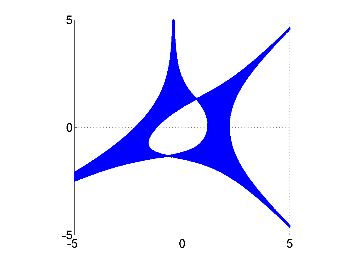
(a)

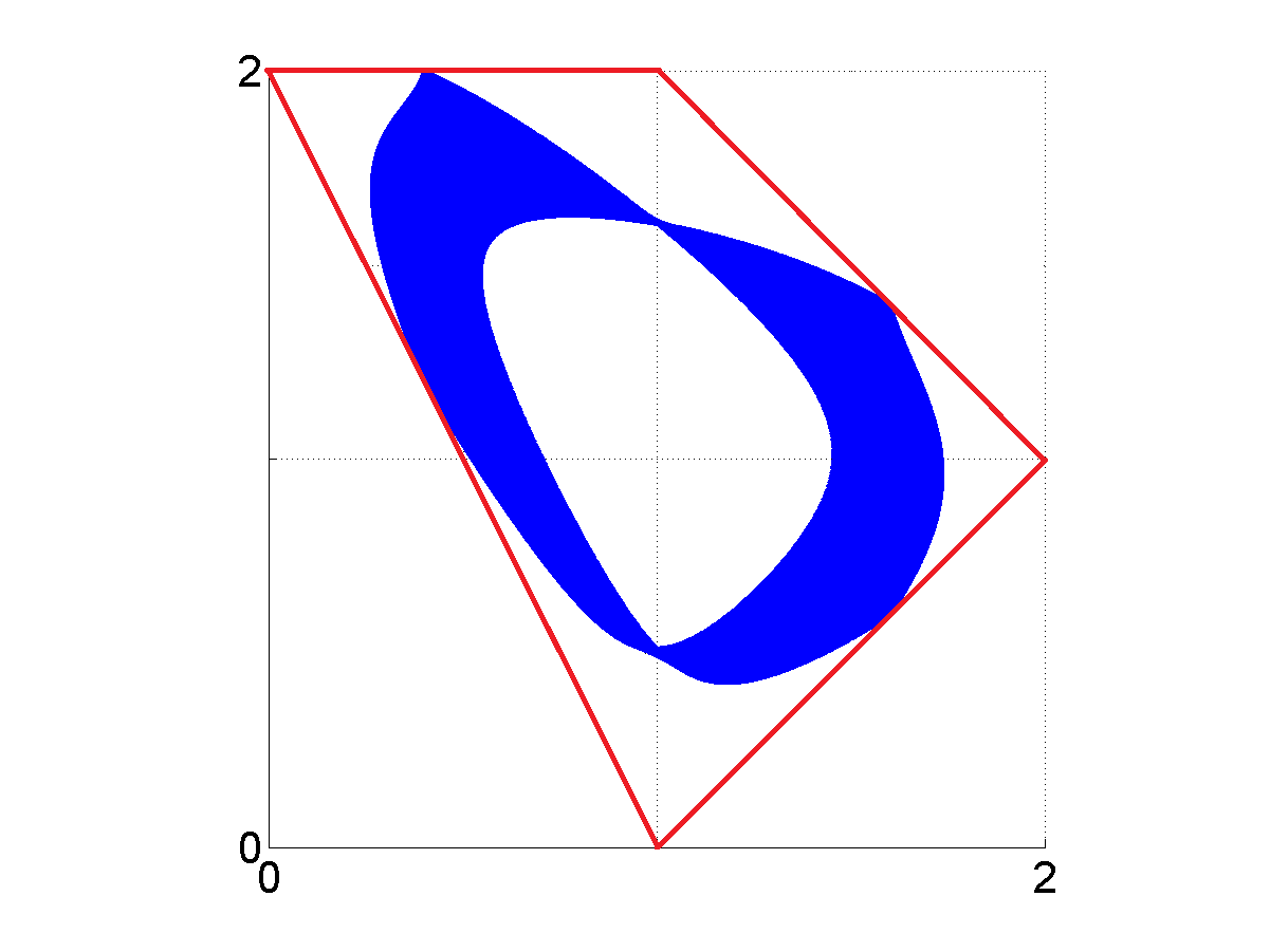
(b)

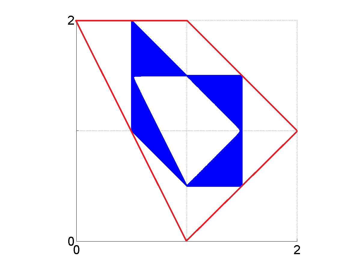
(c)

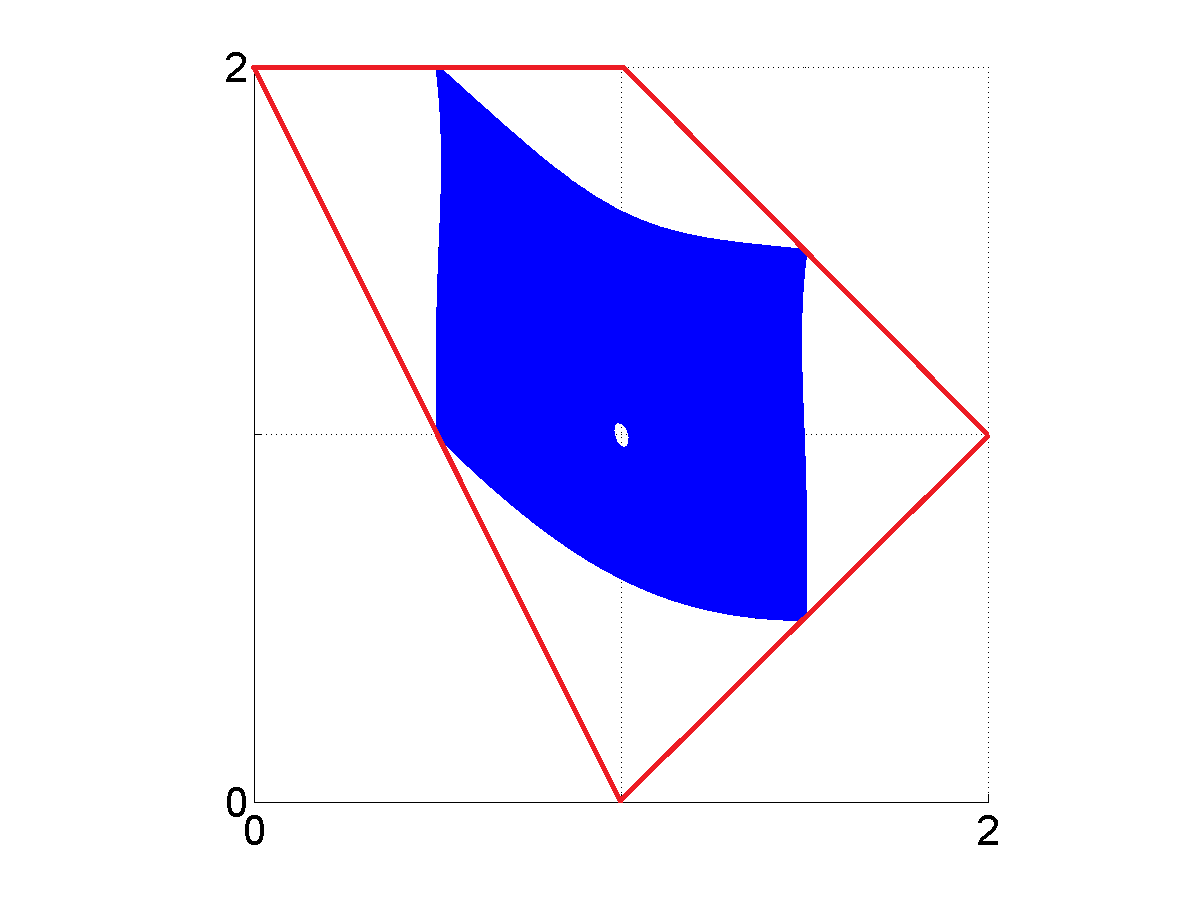
(d)

Figure 4. The amoeba, compactified amoeba, the weighted compactified amoeba of the 6th Hadamard power and a vanishing connected component of the complement to the $\mathcal{WCA}(p_{3}(x,y))$ (see Definition 3.12)

Recall that a (Laurent) polynomial $p(x_{1},\ldots,x_{n})\in\hbox{\Bbb C}[x_{1}^{\pm 1},\ldots,x_{n}^{\pm 1}]$ is called strongly irreducible if for any nondegenerate integer matrix $v$ the polynomial $p(x^{v_{1}},\ldots,x^{v_{n}})$ is irreducible over ℂ. Here $v_{j}$ is the $j$th row of the matrix $v.$ This definition is only meaningful in $n\geq 2$ variables since there are no univariate strongly irreducible polynomials. The property of a polynomial being strongly irreducible in $\hbox{\Bbb C}[x_{1}^{\pm 1},\ldots,x_{n}^{\pm 1}]$ is a generic condition in the Zariski topology. Example 3.9 3) provides a polynomial that is irreducible but is not strongly irreducible.

By Lemma 2.6 the amoeba of a polynomial that is not strongly irreducible is the union of the amoebas of its Puiseux polynomial factors. We thus may without any loss of generality restrict our attention to strongly irreducible hypergeometric polynomials.

The hypergeometric polynomials introduced in Definition 3.7 enjoy properties that are parallel to the properties 1–6 listed in the Introduction of the classical hypergeometric polynomials. Indeed, for any integer convex polytope there is only one (up to a constant multiple) hypergeometric polynomial of the form (3.4) supported in this polytope; this polynomial is dense; it satisfies the hypergeometric system ${\rm Horn}(\psi_{P}(s)).$ The counterpart of the properties of the roots of (3.4) is given by the next theorem which is the main result of the paper.

Theorem 3.10.

Strongly irreducible hypergeometric polynomials are optimal.

Proof.

Let $p(x)$ be a hypergeometric polynomial in the sense of Definition 3.7 with the variables $x=(x_{1},\ldots,x_{n})\in\hbox{\Bbb C}^{n}$ and supported in a finite $\hbox{\Bbb Z}^{n}$-connected set $S\subset\hbox{\Bbb Z}^{n}.$ Denote by $\varphi(s)$ the Ore-Sato coefficient of $p(x).$ By definition, the function $\varphi(s)$ is well-defined, finite and positive on $S.$

By the comment after Remark 3.8 a univariate polynomial that is hypergeometric in the sense of Definition 3.7 is optimal. From now on we will consider the case $n\geq 2.$

By [7], the order of the connected component $M$ of the complement of the amoeba $\mathcal{A}_{f}$ is given by the vector with the coordinates

$$\frac{1}{(2\pi i)^{n}}\int\limits_{\rm{Log}^{-1}(\xi)}\frac{\theta_{j}f(x)}{f(x)}\frac{dx_{1}\wedge\ldots\wedge dx_{n}}{x_{1}\ldots x_{n}},\quad j=1,\ldots,n.$$

Here $\xi$ is any point in $M.$ We will show that for any $\alpha\in S$ there exists a connected component of order $\alpha\in S\subset\hbox{\Bbb Z}^{n}$ in the amoeba complement ${}^{c}\!\mathcal{A}_{p(x)}.$ By Lemma 2.6 it suffices to consider the case when $\alpha$ belongs to the interior of the convex hull (in $\hbox{\Bbb R}^{n}$) of $S.$ Indeed, if $\alpha$ is a vertex of $\mathcal{N}_{p(x)}$ then the desired conclusion is established in Theorem 2.7. If $\alpha$ is on the boundary of the convex hull of $S$ but is not its vertex, then a suitable nondegenerate monomial change of variables can be used to reduce the dimension of the variable space and put $\alpha$ into the interior of the Newton polytope of a polynomial in fewer variables obtained from $p(x)$ by setting some of its variables to zero.

Furthermore, we may without loss of generality assume that $\alpha=0.$ Indeed, by Lemma 2.6 the amoebas of $p(x)$ and $x^{-\alpha}p(x)$ are the same and the component of order $\alpha$ in ${}^{c}\!\mathcal{A}_{p(x)}$ coincides with the component of order $0$ in ${}^{c}\!\mathcal{A}_{x^{-\alpha}p(x)}.$

By the Bohr-Mollerup theorem the coefficient (3.3) of a hypergeometric polynomial is a positive and strictly logarithmically concave function on the convex hull of the support of this polynomial. It follows from [15, Corollary 2] that a sufficiently high positive (integer) power $\ell$ of the Ore-Sato coefficient $\varphi(s)$ defines an optimal hypergeometric polynomial. In fact, any sufficiently big positive real power of $\varphi(s)$ will define an optimal polynomial but it will only satisfy a hypergeometric system of equations for integer powers.

It remains to check that $\ell=1$ works. Let the Ore-Sato coefficient $\psi_{P}(s)$ be defined by (3.3). By definition the function

$$\tilde{p}(x):=\sum\limits_{\tiny\begin{array}[]{c}s\in S\\ s\neq 0\end{array}}\psi_{P}(s)x^{s}$$

is positive and convex in $\hbox{\Bbb R}_{+}^{n}$. It tends to infinity as $x_{j}\rightarrow 0$ or $x_{j}\rightarrow\infty$ for any $j=1,\ldots,n.$ Thus there exists the unique minimum $\rho=(\rho_{1},\ldots,\rho_{n})\in\hbox{\Bbb R}^{n}$ such that $\tilde{p}(x)\geq\tilde{p}(\rho)$ for any $x\in\hbox{\Bbb R}_{+}^{n}.$

Definition 3.11.

Following the ideas of [20], we define the weighted moment map associated with the algebraic hypersurface $\{x\in\hbox{\Bbb C}^{n}:f(x):=\sum\limits_{s\in S}a_{s}x^{s}=0\}$ through

$$\mu_{f}(x):=\frac{\sum\limits_{s\in S}s\cdot|a_{s}||x^{s}|}{\sum\limits_{s\in S}|a_{s}||x^{s}|}.$$

It follows from the general theory of moment maps [9] that $\mu_{f}(\hbox{\Bbb C}^{n})\subseteq\mathcal{N}_{f}.$

Definition 3.12.

By the weighted compactified amoeba of an algebraic hypersurface $H=\{x\in\subset\hbox{\Bbb C}^{n}:f(x)=0\}$ we will mean the set $\mu_{f}(H).$ We denote it by $\mathcal{WCA}(f).$

By [9] there exists a deformation $\hat{p}(x)$ of the Laurent polynomial $\tilde{p}(x)$ such that $\tilde{p}(x)-\hat{p}(x)=\delta\in\hbox{\Bbb R}_{+}$ and moreover the complement of $\mathcal{WCA}(\hat{p}(x)-\varepsilon)$ contains the connected component $M\ni 0\in\hbox{\Bbb R}^{n}$ of order $0\in\hbox{\Bbb Z}^{n}$ for any $\varepsilon\geq 0.$ In other words, there exists a deformation of the constant term of $\tilde{p}(x)$ which makes the complement component of order zero vanish at the origin. This is illustrated by Fig. 4 (d) and 9 (d).

It is therefore sufficient to check that the origin cannot belong to $\mathcal{WCA}(\tilde{p}(x)).$ The preimage of the origin under the map $\mu_{\tilde{p}}$ is given by

$$\Pi=\left\{x\in\hbox{\Bbb C}^{n}:\frac{\partial\tilde{p}(\zeta)}{\partial\zeta_{j}}\Big{|}_{\zeta_{1}=|x_{1}|,\ldots,\zeta_{n}=|x_{n}|}=0\text{\ for\ any\ }j=1,\ldots,n\right\}.$$

Since the only point in $\hbox{\Bbb R}_{+}^{n}$ where the gradient of $\tilde{p}(x)$ vanishes is $\rho,$ it follows, that

$$\Pi=\left\{(\rho_{1}e^{i\chi_{1}},\ldots,\rho_{n}e^{i\chi_{n}}):\chi_{j}\in[0,2\pi]\right\}.$$

To prove the existence of the complement component of order zero we need to show that the Laurent polynomial $\tilde{p}(x)$ cannot vanish on $\Pi.$

Consider the set $\mathcal{L}$ of lines in $\hbox{\Bbb R}^{n}$ such that the intersection of any element in $\mathcal{L}$ with $S$ contains three points. If $\mathcal{L}$ is empty then the polynomial $\tilde{p}(x)$ is optimal by [7]. From now on we assume that $\mathcal{L}$ is nonempty. Let $L\in\mathcal{L}$ and consider the restricted polynomial $p|_{L}(x):=\sum\limits_{s\in S\cap L}\varphi(s)x^{s}.$ Since the coefficients of $p(x)$ are defined as the restriction of a logarithmically concave function to the support of $p(x),$ the same is true for the coefficients of the restricted polynomial $p|_{L}(x).$ Making, if necessary, a monomial change of variables, we conclude that $p|_{L}(x)=a_{L}m(x)^{2}+b_{L}m(x)+c_{L},$ where $a_{L},b_{L},c_{L}\in\hbox{\Bbb Z}$ and $m(x)$ is a monomial function in the coordinates of $x.$ Moreover, this second-order polynomial has a logarithmically concave hypergeometric coefficient and vanishes on a certain circle centered at the origin.

The logarithmic concavity of the coefficient of $p|_{L}(x)$ is equivalent to $b_{L}\geq\sqrt{a_{L}c_{L}}.$ Since the coefficients of $p|_{L}(x)$ are positive integers, its roots are on the same circle centered at the origin if and only if $p|_{L}(x)=a_{L}m(x)^{2}-2a_{L}m(\rho)\cos\omega\,m(x)+a_{L}m(\rho)^{2},$ where $\cos\omega\leq\frac{1}{2}.$ Such a polynomial can only be a restriction of a multivariate hypergeometric polynomial in the case when $\omega=\pi$ and its roots are the same. If this holds for any $L\in\mathcal{L}$ then the initial polynomial $p(x)$ cannot be strongly irreducible.

This means that there is a connected component of order $\alpha$ in the complement of the amoeba $\mathcal{A}_{p(x)}.$ Since $\alpha\in S\subset\hbox{\Bbb Z}^{n}$ was arbitrary, the amoeba is optimal. ∎

We stress once again that by Definition 3.7 the optimality of a polynomial is the property of its zero locus and not the polynomial itself. For instance, the bivariate hypergeometric polynomial $(1-x-y)^{2}$ is optimal since its zeros form the optimal algebraic hypersurface $\{x+y=1\}.$

The class of dense optimal multivariate polynomials with $\hbox{\Bbb Z}^{n}$-convex supports is of course much wider than the class of hypergeometric polynomials. By [15] the coefficient of a polynomial only has to be ”logarithmically concave enough” for the polynomial itself to be optimal.

Example 3.9 (a) shows that the condition of (strong) irreducibility is in general not necessary for a hypergeometric polynomial to be optimal. On the other hand, the polynomial in Example 3.9 (c) fails the strong irreducibility condition and is not optimal due to the fact that it factors into the product of two different Puiseux polynomials with the same amoebas. Throughout the rest of the paper we will without loss of generality only consider strongly irreducible hypergeometric polynomials.

Example 3.13.

The bivariate Ore-Sato coefficient

$$\varphi(s,t)=\left(\Gamma(t+1)\Gamma(1+6s-3t)\Gamma(31-6s-2t)\right)^{-1}$$

defines a confluent holonomic hypergeometric system with the polynomial solution

$$\begin{array}[]{c}p_{0}(x,y)=1+593775x+86493225x^{2}+86493225x^{3}+593775x^{4}+x^{5}+39331656000xy+\\ 34936343442000x^{2}y+55898149507200x^{3}y+216324108000x^{4}y+54513675216000xy^{2}+\\ 2112950051372160000x^{2}y^{2}+6867087666959520000x^{3}y^{2}+10357598291040000x^{4}y^{2}+\\ 15382276373989324800000x^{2}y^{3}+169205040113882572800000x^{3}y^{3}+\\ 33807200821954560000x^{4}y^{3}+3045690722049886310400000x^{2}y^{4}+\\ 639595051630476125184000000x^{3}y^{4}+184203374869577124052992000000x^{3}y^{5}+\\ 368406749739154248105984000000x^{3}y^{6}.\end{array}$$

The support of this hypergeometric polynomial is $\hbox{\Bbb Z}^{2}$-convex and has a triangular convex hull. The amoeba of $p_{0}(x,y)$ is optimal, see Fig. 5.

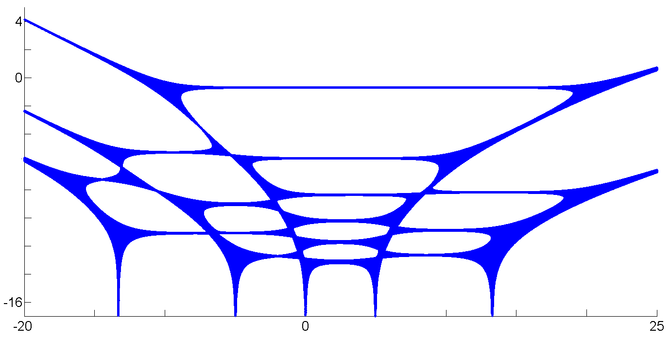
Figure 5. The Newton polygon and the amoeba of $p_{0}(x,y)$

Remark 3.14.

Recall that the Bergman kernel of a complex ellipsoidal domain is given by a rational hypergeometric function [13]. One can check that the numerators of such rational functions are not necessarily optimal polynomials. The amoebas of the singular divisors of the GKZ-hypergeometric functions [2] are known to be solid [13]. Thus the optimal property of the divisors of hypergeometric polynomials cannot be extended to the classes of rational or algebraic hypergeometric functions.

Recall that the Hadamard power of order $r\in\hbox{\Bbb R}$ of a polynomial $f(x)=\sum\limits_{s\in S}a_{s}x^{s}$ is defined to be $f^{[r]}(x):=\sum\limits_{s\in S}a_{s}^{r}x^{s}.$ We observe that the set-theoretical limit $\mathcal{S}(f):=\lim\limits_{r\rightarrow\infty}\mathcal{WCA}(f^{[r]})\subset\mathcal{N}_{f}$ is an amoeba-like simplicial complex. This simplicial complex for the Hirzebruch polynomial is depicted in Fig. 4 (c) inside the Newton polygon of that polynomial. An approximation of the simplicial complex $\mathcal{S}(p_{3}(x,y))$ is depicted in Fig. 9 (c). The geometry of $\mathcal{S}(f)$ is related to the amoeba of $f$ while the combinatorics of $\mathcal{S}(f)$ reflects intrinsic algebraic properties of this polynomial.

4. Classical bivariate hypergeometric polynomials

Despite varying terminology, the classical hypergeometric series $F_{1},\ldots,F_{4},$ $G_{1},\ldots,G_{3},$ $H_{1},\ldots,H_{7}$ as well as other entries of the Horn list [6] are universally considered to be intrinsically hypergeometric. For resonant parameters [18], many of these series terminate and turn out to be bivariate hypergeometric polynomials.

Appell’s $F_{1}$ is one of the most important classical hypergeometric series since by the results of [6] any bivariate hypergeometric system of second-order equations and holonomic rank 3 can be transformed into the system for $F_{1}$ or a particular limiting case of this system. The following statement follows from Theorem 3.10.

Corollary 4.1.

The polynomial instances of the Appell $F_{1}(a,b_{1},b_{2},c;x,y)$ hypergeometric function are optimal for $a,b_{1},b_{2},-c<0$ and $a>b_{1}+b_{2}.$

Proof.

The imposed conditions on the parameters of $F_{1}(a,b_{1},b_{2},c;x,y)$ yield a one-to-one correspondence between the $\Gamma$-factors in the coefficient of the power series expansion of $F_{1}$ and the sides of the Newton polygon of its polynomial instance in question. This polynomial is therefore hypergeometric in the sense of Definition 3.7. ∎

In Fig. 6 we depict the amoeba of the optimal hypergeometric polynomial $F_{1}(-5,-4,-4,$ $3;x,y).$

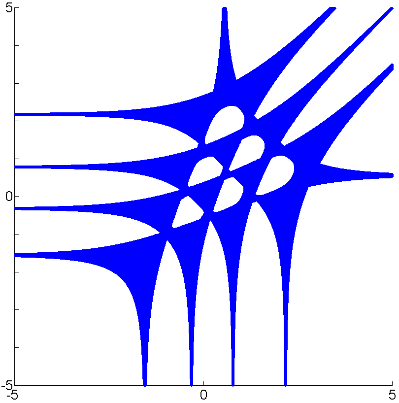
Figure 6. The Newton polygon and the amoeba of the Appell polynomial $F_{1}(-5,-4,-4,3;x,y)$

Observe however that not every polynomial instance of $F_{1}(a,b_{1},b_{2},c;x,y)$ is optimal. The optimal property is in general not possessed by the $F_{1}$ polynomials whose Newton polytopes do not have sides that are orthogonal to the gradients of the linear forms in the defining Ore-Sato coefficient. For instance, $F_{1}(-4,5,-7,9;x,y)$ is not an optimal polynomial, its Newton polygon being just a triangle.

We further remark that the zero locus of a rational instance of a classical hypergeometric function need not be an optimal hypersurface. For example, the numerator of the rational function $F_{2}(5;3/2,1;-1/2,2;x,y)$ is not an optimal polynomial.

5. examples

In this section we collect examples of multivariate hypergeometric polynomials together with their Newton polytopes and amoebas.

Example 5.1.

The hypergeometric Horn system defined by the Ore-Sato coefficient

$$\varphi(s,t)=\Gamma(s-6)\Gamma(s+t-10)\Gamma(t-6)\Gamma(-s+t-4)\Gamma(-s)\Gamma(-s-t+2)\Gamma(-t)\Gamma(s-t-4)$$

admits the following polynomial solution:

$p_{1}(x,y)=21x^{2}+64x^{3}+21x^{4}+126xy+2016x^{2}y+4704x^{3}y+2016x^{4}y+126x^{5}y+21y^{2}+2016xy^{2}+22050x^{2}y^{2}+47040x^{3}y^{2}+22050x^{4}y^{2}+2016x^{5}y^{2}+21x^{6}y^{2}+64y^{3}+4704xy^{3}+47040x^{2}y^{3}+98000x^{3}y^{3}+47040x^{4}y^{3}+4704x^{5}y^{3}+64x^{6}y^{3}+21y^{4}+2016xy^{4}+22050x^{2}y^{4}+47040x^{3}y^{4}+22050x^{4}y^{4}+2016x^{5}y^{4}+21x^{6}y^{4}+126xy^{5}+2016x^{2}y^{5}+4704x^{3}y^{5}+2016x^{4}y^{5}+126x^{5}y^{5}+21x^{2}y^{6}+64x^{3}y^{6}+21x^{4}y^{6}.$

(The system itself is too cumbersome to display and we omit it.) The Newton polygon and the amoeba of $p_{1}(x,y)$ are shown in Fig. 7. This amoeba turns out to be optimal.

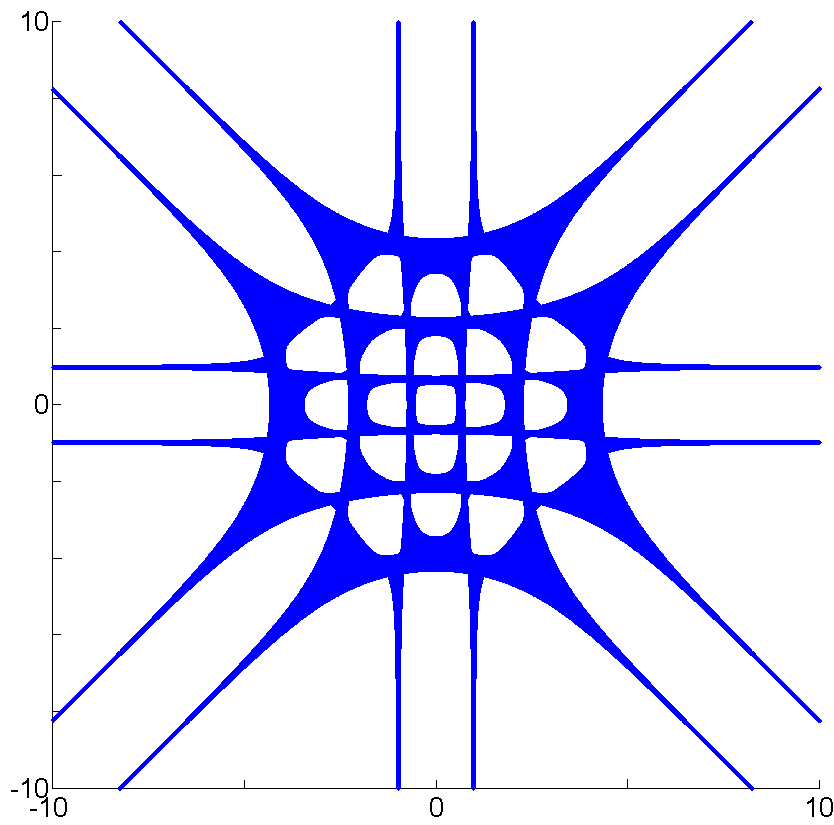
Figure 7. The Newton polygon and the amoeba of $p_{1}(x,y)$

Example 5.2.

The next example shows that the number of $\Gamma$-factors in the Ore-Sato coefficient of an optimal hypergeometric polynomial can be strictly smaller than the number of faces of its Newton polytope. The hypergeometric system defined by the Ore-Sato coefficient

(5.1) $$\varphi(s,t)=\Gamma\left(s+2t-5\right)\Gamma\left(-2s-t-4\right)\Gamma\left(-s-5t+1\right)$$

has the following polynomial solution:

$p_{2}(x,y)=2421619200x^{5}+172972800x^{6}+2882880x^{7}+14560x^{8}+20x^{9}+174356582400x^{2}y+48432384000x^{3}y+2421619200x^{4}y+34594560x^{5}y+160160x^{6}y+208x^{7}y+2421619200xy^{2}+691891200x^{2}y^{2}+21621600x^{3}y^{2}+160160x^{4}y^{2}+286x^{5}y^{2}+524160xy^{3}+14560x^{2}y^{3}+56x^{3}y^{3}+32y^{4}+xy^{4}.$

The support of $p_{2}(x,y)$ (bounded by the singular divisors of the corresponding Ore-Sato coefficient) and its amoeba are depicted in Fig. 8.

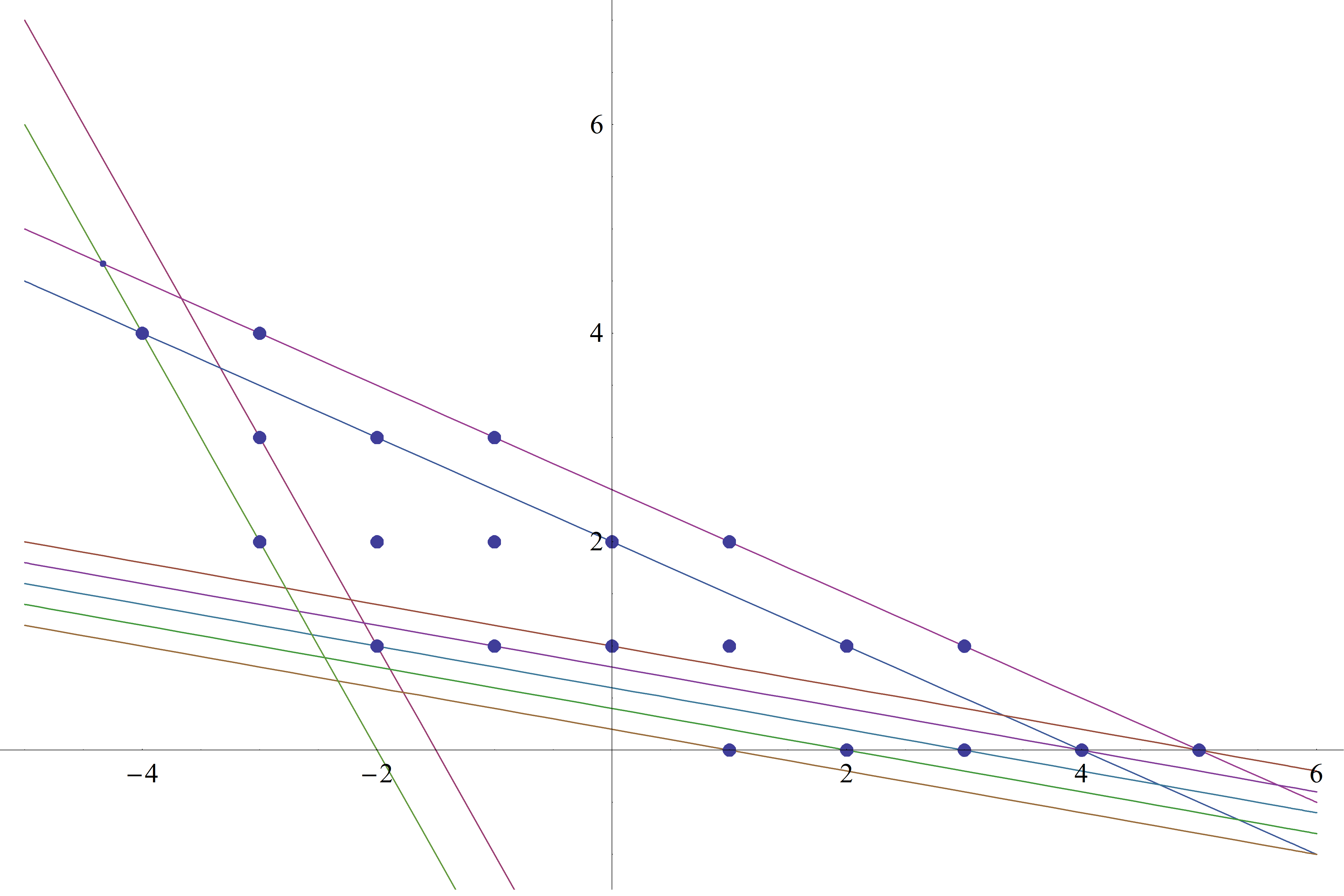
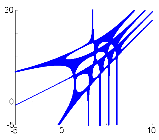
Figure 8. The support of $p_{2}(x,y)$ (bounded by the singular divisors of (5.1)) and its amoeba

Example 5.3.

The bivariate hypergeometric polynomial supported in the quadrilateral with the vertices $(2,0),(3,2),(2,3)$ and $(0,1)$ is given by $p_{3}(x,y)=240x^{2}+3y+240xy+1080x^{2}y+30xy^{2}+180x^{2}y^{2}+36x^{3}y^{2}+2x^{2}y^{3}.$ Fig. 9 (a-c) show the affine amoeba $\mathcal{A}_{p_{3}}$, the compactified amoeba of $p_{3}(x,y)$, the weighted compactified amoeba of the 6th Hadamard power of $p_{3}(x,y).$ Fig. 9 (d) shows the vanishing connected component with the order $(2,2)$ in the complement of the weighted compactified amoeba of a deformed version of $p_{3}(x,y).$ We remark that the small component vanishes exactly at the point with the coordinates $(2,2),$ that is, at the order of this component.

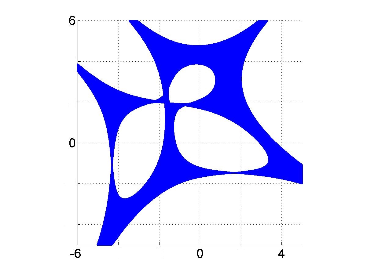
(a)

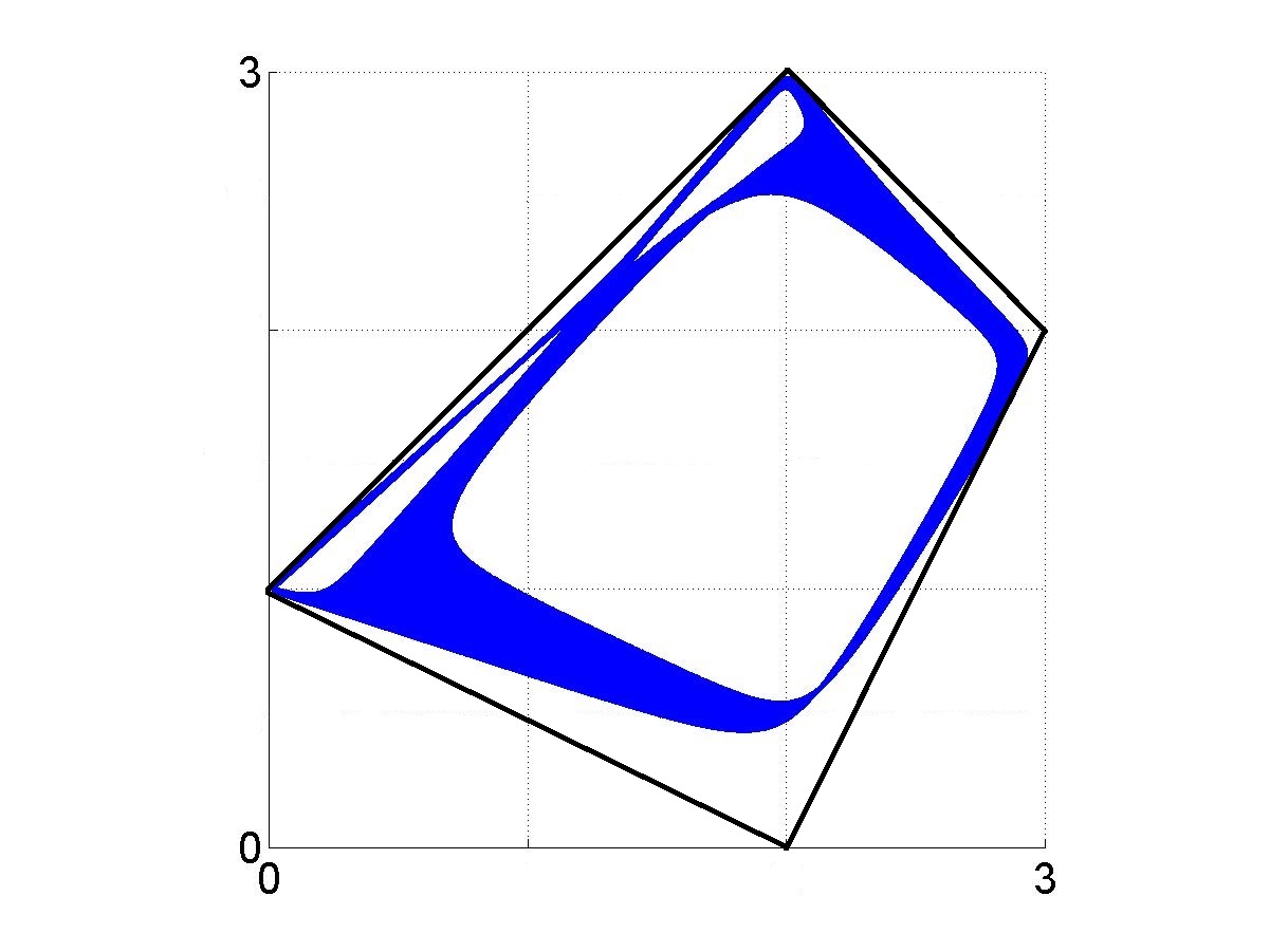
(b)

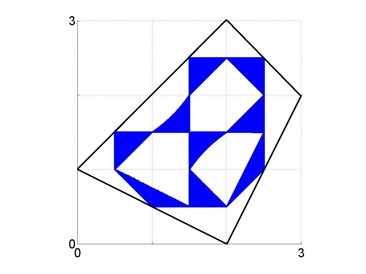
(c)

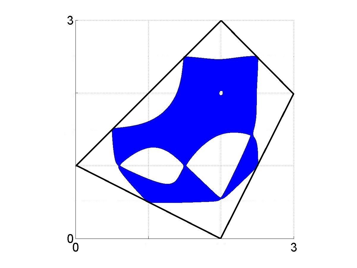
(d)

Figure 9. The amoeba, compactified amoeba, the weighted compactified amoeba of the 6th Hadamard power and a vanishing connected component of the complement to the $\mathcal{WCA}(p_{3}(x,y))$

Example 5.4.

The first maximal minor of the Toeplitz matrix

$$\left(\begin{array}[]{ccccccc}x&y&1&0&0&0&0\\ 1&x&y&1&0&0&0\\ 0&1&x&y&1&0&0\\ 0&0&1&x&y&1&0\\ 0&0&0&1&x&y&1\\ 0&0&0&0&1&x&y\end{array}\right)$$

is the degree 6 bivariate Chebyshev polynomial of the second kind [1]. It is optimal in the coordinates $\xi=xy,\,\eta=y^{2}/x$ which make it dense.

References

- [1] P. Alexandersson and B. Shapiro. Around a multivariate Schmidt-Spitzer theorem, Linear Alg. Appl. 446, no. 1 (2014), 356-368.
- [2] F. Beukers. Algebraic A-hypergeometric functions, Invent. Math. 180, no. 3 (2010), 589-610.
- [3] D. Dominici, S.J. Johnston, and K. Jordaan. Real zeros of hypergeometric polynomials, Journal of Comput. and Appl. Math. 247 (2013), 152-161.
- [4] K.A. Driver and S.J. Johnston. Asymptotic zero distribution of a class of hypergeometric polynomials, Quaestiones Mathematicae 30, no. 2 (2007), 219-230.
- [5] C.F. Dunkl and Y. Xu. Orthogonal Polynomials of Several Variables. Cambridge University Press, 2014.
- [6] A. Erdelyi. Hypergeometric functions of two variables, Acta Math. 83 (1950), 131-164.
- [7] M. Forsberg, M. Passare, and A. K. Tsikh. Laurent determinants and arrangements of hyperplane amoebas, Adv. Math. 151 (2000), 45-70.
- [8] I.M. Gelfand, M.I. Graev, and V.S. Retach. General hypergeometric systems of equations and series of hypergeometric type, Russian Math. Surveys 47, no. 4 (1992), 1-88.
- [9] V. Guillemin and S. Sternberg. Convexity properties of the moment mapping, Invent. Math. 67, no. 3 (1982), 491-513.
- [10] F. Klein. Über die Nullstellen der hypergeometrischen Reihe, (German) Math. Ann. 37, no. 4 (1890), 573-590.
- [11] G. Mikhalkin. Real algebraic curves, the moment map and amoebas, Ann. Math. (2) 151, (2000) 309-326.
- [12] N.E. Nørlund. Hypergeometric functions, Acta Math. 94 (1955), 289-349.
- [13] M. Passare, T.M. Sadykov, and A.K. Tsikh. Nonconfluent hypergeometric functions in several variables and their singularities, Compos. Math. 141, no. 3 (2005), 787-810.
- [14] K. Purbhoo. A Nullstellensatz for amoebas, Duke Math. J. 141, no. 3 (2008), 407-445.
- [15] H. Rullgård. Stratification des espaces de polynômes de Laurent et la structure de leurs amibes (French), Comptes Rendus de l’Academie des Sciences - Series I: Mathematics 331, no. 5 (2000), 355-358.
- [16] T.M. Sadykov. On a multidimensional system of hypergeometric differential equations, Siberian Math. J. 39 (1998), 986-997.
- [17] T.M. Sadykov. On the Horn system of partial differential equations and series of hypergeometric type, Math. Scand. 91 (2002), 127-149.
- [18] T.M. Sadykov and S. Tanabe. Maximally reducible monodromy of bivariate hypergeometric systems, Izv. Math. 80, no. 1, (2016), 221-262.
- [19] T. Theobald and T. de Wolff. Amoebas of genus at most one, Adv. Math. 239 (2013), 190-213.
- [20] I. Zharkov. Torus fibrations of Calabi-Yau hypersurfaces in toric varieties, Duke Math. J. 101, no. 2 (2000), 237-257.
- [21] J.-R. Zhou, H.M. Srivastava, and Z.-G. Wang. Asymptotic distribution of the zeros of a family of hypergeometric polynomials, Proc. of the AMS, 140, no. 7 (2012), 2333-2346.
- [22]