Spectral Gap of the Anti-Ferromagnetic Lipkin-Meshkov-Glick Model

Abstract

The spectral property of the supersymmetric (SUSY) antiferromagnetic Lipkin-Meshkov-Glick (LMG) model with an even number of spins is studied. The supercharges of the model are explicitly constructed. By using the exact form of the supersymmetric ground state we introduce simple trial variational states for first excited states. It is demonstrated numerically that they provide a relatively accurate upper bound for the spectral gap (the energy difference between the ground state and first excited states) in all parameter ranges. However, being an upper bound, it does not allow us to determine vigorously whether the model is gapped or gapless. Here, we provide a non-trivial lower bound for the spectral gap and thereby show that the antiferromagnetic SUSY LMG model is gapped for any even number of spins.

I
Introduction

About fifty years ago, an exactly solvable model of interacting fermions was introduced in nuclear physics by Lipkin, Meshkov and Glick Lipkin . This model has been subsequently found widespread use not only in nuclear physics, but also to a variety of other fields of physics, such as Bose–Einstein condensates Cirac , ion traps Unanyan2003 and cavities Larson . The Lipkin, Meshkov and Glick (LMG) Hamiltonian reads

$$H=\xi\left(\chi_{1}^{2}J_{x}^{2}+\chi_{2}^{2}J_{y}^{2}+\lambda\chi_{1}\chi_{2}J_{z}\right),$$ (1)

where $J_{i}=\frac{1}{2}{\displaystyle\sum\limits_{n=1}^{N}}\sigma_{i}^{\left(n\right)}$, $i=x,y,z$, are the familiar angular momentum operators, $\sigma_{i}^{\left(n\right)}$ are the Pauli matrices, $N$ is the total spin number. In the present paper, we focus our attention on the manifold with maximum angular momentum $J=N/2$, where $N$ is an even integer. So the Hilbert space has dimension $2J+1$. The parameters $\chi_{1,2},$ and $\lambda$ are assumed to be positive constants. At the point where $\chi_{2}=0$, the ground state of the Hamiltonian (1) is either ferromagnetic or antiferromagnetic depending on the sign of $\xi$. In the present paper we discuss the antiferromagnetic case ($\xi>0$) and without loss of generality, we set $\xi=1$. We notice that the rotation  $\exp\left(i\frac{\pi}{2}J_{x}\right)$ transforms the Hamiltonian (1) into the form $\chi_{1}^{2}J_{y}^{2}+\chi_{2}^{2}J_{x}^{2}+\lambda\chi_{1}\chi_{2}J_{z}$  and therefore, we may assume that $\chi_{1}\geq\chi_{2}$.

As has been observed in refs.Unanyan2003 the spectrum of the model (1) at $\lambda=1$ presents a two-fold degeneracy in the excited spectrum and non degenerate ground state with zero energy. These observations manifest the presence of the supersymmetry (SUSY) in the system. As far as the author knows, there is still no mathematical proof that the Hamiltonian (1) is supersymmetric and existence of a non-vanishing spectral gap (the energy difference between the ground state and first excited states) in the spectrum at $\lambda=1$. The aim of this paper is to present a detailed proof of these observations.

First, we show that the LMG model at $\lambda=1$ is indeed supersymmetric by constructing the supercharges $Q_{1}$ and $Q_{2}$

$$H=Q_{1}^{2}=Q_{2}^{2},$$ (2)

and show that they anticommute, that is

$$\left\{Q_{1},Q_{2}\right\}=0.$$ (3)

For a good introduction to the SUSY the reader is referred to review articles e.g. Witten . One consequence of this result is that it automatically yields the two-fold degeneracy of excited states Witten . Analogous results are known as a result of elaborate approximative WKB computations Garg .

Second, we obtain upper and lower bounds for the spectral gap $\Delta E$ i.e. the first excited state energy (since the ground state energy is zero) of the Hamiltonian (1). We show that a knowledge of the ground state allows us to obtain a reasonable upper bound for the spectral gap by using relatively simple variational states. The obtained bounds grow with the system size. As a rule, the variational estimates are usually in good agreement with exact eigenvalues of a Hamiltonian. Hence, it is natural to expect that the true spectral gap of the antiferromagnetic SUSY LMG model would also grow with $J$. We confirm this numerically and, moreover, provide a non-trivial lower bound for the first excited state energy. So we rigorously prove that the system (1) at the supersymmetric point is indeed gapped for any integer value of $J$.

II Supersymmetry in the LMG model

The analysis of the spectrum of the Hamiltonian (1) can be greatly simplified by introducing a new set of variables $\Omega_{0}$ and $\gamma$:

$$\chi_{1} =\Omega_{0}\cosh\gamma,$$ (4)

$$\chi_{2} =\Omega_{0}\sinh\gamma,$$

where

$$\Omega_{0}^{2}=\chi_{1}^{2}-\chi_{2}^{2}\text{ \ and }\tanh\gamma=\frac{\chi_{2}}{\chi_{1}}.$$ (5)

The Hamiltonian (1) can be factorized by making use of the identity

$$\exp\left(-\gamma J_{z}\right)J_{x}\exp\left(\gamma J_{z}\right)=J_{x}\cosh\gamma-iJ_{y}\sinh\gamma$$ (6)

for a hyperbolic rotation around the $z$ -axis with the parameter $\gamma$ as follows

$$H=\Omega_{0}^{2}\left(J_{x}\cosh\gamma+iJ_{y}\sinh\gamma\right)\left(J_{x}\cosh\gamma-iJ_{y}\sinh\gamma\right)=$$

$$=\Omega_{0}^{2}\exp\left(-\gamma J_{z}\right)J_{x}\exp\left(2\gamma J_{z}\right)J_{x}\exp\left(-\gamma J_{z}\right).$$ (7)

It can easily be seen from Eq. (7) that for arbitrary values of $\gamma$ all eigenvalues of the Hamiltonian (7) are non-negative $E\geq 0$. Notice that the unitary transformation $\exp\left(i\pi J_{x}\right)$ changes the operator $J_{z}\rightarrow-J_{z}$ and therefore the spectrum of the Hamiltonian  is symmetric with respect to $\gamma\rightarrow-\gamma$. Hence, it is sufficient to restrict ourselves to the consideration of positive $\gamma$. One purpose of this paper is to show that the LMG model (1) at $\lambda=1$ is supersymmetric.  Instead of defining $Q_{1,2}$ operators in terms of fermionic operators, we give their block-matrix representation in the two invariant subspaces labeled by the ”fermionic” number operator $F=\frac{1}{2}\left({{1\!\!1}}+e^{i\pi\left(J_{z}+J\right)}\right)$.  The operator $F$ has two distinct eigenvalues $0$ and $1$ with multiplicities $J+1$ and $J$ respectively. It is easily seen that, the matrices

$$Q_{1}=\left(\begin{array}[c]{cc}\underset{\left(J+1\right)\times\left(J+1\right)}{\underbrace{0}}&\underset{\left(J+1\right)\times\left(J\right)}{\underbrace{B}}\\ \underset{\left(J\right)\times\left(J+1\right)}{\underbrace{B^{\dagger}}}&\underset{J\times J}{\underbrace{0}}\end{array}\right),\text{ \ \ \ }Q_{2}=\left(\begin{array}[c]{cc}\underset{\left(J+1\right)\times\left(J+1\right)}{\underbrace{0}}&\underset{\left(J+1\right)\times\left(J\right)}{\underbrace{-iB}}\\ \underset{\left(J\right)\times\left(J+1\right)}{\underbrace{iB^{\dagger}}}&\underset{J\times J}{\underbrace{0}}\end{array}\right),$$ (8)

where

$$B_{m_{1},m_{2}}=\Omega_{0}\left\langle m_{1}\right|\left(J_{x}\cosh\gamma+iJ_{y}\sinh\gamma\right)\left|m_{2}\right\rangle,$$ (9)

$$m_{1}=J,J-2,...-J,\text{ \ }m_{2}=J-1,J-3,...-\left(J-1\right)$$

fulfill the anticommutation relation (3). The symbol $\underset{\left(M\right)\times\left(N\right)}{\underbrace{X}}$ denotes a $M\times N$ matrix. We show that the relations (2) also hold for these matrices. Indeed,

$$Q_{1}^{2}=Q_{1}^{2}=\left(\begin{array}[c]{cc}\underset{\left(J+1\right)\times\left(J+1\right)}{\underbrace{BB^{\dagger}}}&\underset{\left(J+1\right)\times\left(J\right)}{\underbrace{0}}\\ \underset{\left(J\right)\times\left(J+1\right)}{\underbrace{0}}&\underset{J\times J}{\underbrace{B^{\dagger}B}}\end{array}\right),$$

and according to (9), for $m_{1},n_{1}=J,J-2,...-J$ we have

$$\left(BB^{\dagger}\right)_{m_{1},n_{1}}=\Omega_{0}^{2}{\displaystyle\sum\limits_{m_{2}=J-1,...,-\left(J-1\right)}}\left\langle m_{1}\right|\left(J_{x}\cosh\gamma+iJ_{y}\sinh\gamma\right)\left|m_{2}\right\rangle\left\langle m_{2}\right|\left(J_{x}\cosh\gamma-iJ_{y}\sinh\gamma\right)\left|n_{1}\right\rangle$$

By inserting the resolution of identity

$${\displaystyle\sum\limits_{m=-\left(J-1\right),-\left(J-3\right),...\left(J-1\right)}}\left|m\right\rangle\left\langle m\right|={1\!\!1-}{\displaystyle\sum\limits_{m=-J,-J+2,...J}}\left|m\right\rangle\left\langle m\right|$$

into the sum, we can write

$$\left(BB^{\dagger}\right)_{m_{1},n_{1}}=\Omega_{0}^{2}\left\langle m_{1}\right|\left(J_{x}^{2}\cosh^{2}\gamma+J_{y}^{2}\sinh^{2}\gamma+J_{z}\sinh\gamma\cosh\gamma\right)\left|n_{1}\right\rangle-$$

$$-\Omega_{0}^{2}{\displaystyle\sum\limits_{m=J,J-2,...,-J}}\left\langle m_{1}\right|\left(J_{x}\cosh\gamma+iJ_{y}\sinh\gamma\right)\left|m\right\rangle\left\langle m\right|\left(J_{x}\cosh\gamma-iJ_{y}\sinh\gamma\right)\left|n_{1}\right\rangle=$$

$$\Omega_{0}^{2}\left\langle m_{1}\right|\left(J_{x}^{2}\cosh^{2}\gamma+J_{y}^{2}\sinh^{2}\gamma+J_{z}\sinh\gamma\cosh\gamma\right)\left|n_{1}\right\rangle\text{.}$$

In the last line we have used the fact $\left\langle m_{1}\right|\left(J_{x}\cosh\gamma+iJ_{y}\sinh\gamma\right)\left|m\right\rangle=0$, for any $m_{1},m$ from the set $\left\{J,J-2,...-J+2,-J\right\}$.

Analogously, for any $m_{2},n_{2}$ from the set $\left\{J-1,J-3,...-\left(J-1\right)\right\}$ one has

$$\left(B^{\dagger}B\right)_{m_{2},n_{2}}=\Omega_{0}^{2}\left\langle m_{2}\right|\left(J_{x}^{2}\cosh^{2}\gamma+J_{y}^{2}\sinh^{2}\gamma+J_{z}\sinh\gamma\cosh\gamma\right)\left|n_{2}\right\rangle.$$

Combining these two expressions the Hamiltonian (1) in the eigenbasis of $F$ can be partitioned into the block-diagonal form

$$H=\Omega_{0}^{2}\left(\begin{array}[c]{cc}\underset{\left(J+1\right)\times\left(J+1\right)}{\underbrace{J_{x}^{2}\cosh^{2}\gamma+J_{y}^{2}\sinh^{2}\gamma+J_{z}\sinh\gamma\cosh\gamma}}&\underset{\left(J+1\right)\times\left(J\right)}{\underbrace{0}}\\ \underset{\left(J\right)\times\left(J+1\right)}{\underbrace{0}}&\underset{J\times J}{\underbrace{J_{x}^{2}\cosh^{2}\gamma+J_{y}^{2}\sinh^{2}\gamma+J_{z}\sinh\gamma\cosh\gamma}}\end{array}\right).$$

Hence, we have proved that the Hamiltonian (1) is supersymmetric at $\lambda=1$.

The factorized form (7) allows us  to write the normalized ground state of (1) in the following explicit form

$$\left|\Psi_{g}\right\rangle=\frac{1}{\sqrt{P_{J}\left(\cosh 2\gamma\right)}}\exp\left(\gamma J_{z}\right)\left|m_{x}=0\right\rangle,$$ (10)

with $P_{J}\left(x\right)$ being Legendre polynomials. Where, $\left|m_{i}=m\right\rangle$ , $i=x,y,z$ denotes eigenvector of $J_{i}$ associated with the magnetic quantum number $m$. For the excited states, however, no further information can be gotten from the SUSY algebra (2) and (3), besides that they are two-fold degenerate. However, as we will show below the explicit form of the ground state can be used to find an accurate upper bound on the spectral gap.

III Upper bounds for the spectral gap

When the ground state is known, an upper bound to the spectral gap $\Delta E$, can be found from the following inequality Eckert

$$\Delta E\leq\frac{\left\langle\Phi\right|H\left|\Phi\right\rangle}{1-\left|\left\langle\Phi\right|\left.\Phi_{g}\right\rangle\right|^{2}},$$ (11)

where $\left|\Phi_{g}\right\rangle$  and $\left|\Phi\right\rangle$ are normalized ground and trial wave functions respectively.

For purposes of calculation it is convenient to transform the Hamiltonian (7) into a unitarily equivalent

$$H =\Omega_{0}^{2}\left(J_{z}^{2}\cosh^{2}\gamma+J_{y}^{2}\sinh^{2}\gamma-J_{x}\sinh\gamma\cosh\gamma\right)=$$ (12)

$$\Omega_{0}^{2}\exp\left(-\gamma J_{x}\right)J_{z}\exp\left(2\gamma J_{x}\right)J_{z}\exp\left(-\gamma J_{x}\right),$$

form.

Guided by our physical intuition, we choose the following trial state vector

$$\left|\Phi_{0}\right\rangle=\frac{\exp\left(-\gamma J_{x}\right)}{\sqrt{\left\langle+\right|\exp\left(-2\gamma J_{x}\right)\left|+\right\rangle}}\left|+\right\rangle,$$ (13)

where

$$\left|+\right\rangle=\frac{1}{\sqrt{2}}\left(\left|m_{z}=1\right\rangle+\left|m_{z}=-1\right\rangle\right).$$ (14)

This choice is dictated by the following circumstances: First, for small and large $\gamma$, it coincides with the first excited state of the Hamiltonian (12). Indeed, it is straightforward to show that the Hamiltonian (12) for these two limiting cases becomes simple form

$$H\approx\left\{\begin{array}[c]{c}\Omega_{0}^{2}J_{z}^{2}\text{ \ if }\gamma\rightarrow 0\\ \Omega_{0}^{2}\frac{\exp\left(2\gamma\right)}{4}\left(J(J+1-J_{x}\left(J_{x}+1\right)\right)\text{ if }\gamma\rightarrow\infty.\end{array}\right.$$ (15)

It is clear from (13) that for large $\left(\delta=\gamma J>>1\right)$ the state $\left|\Phi_{0}\right\rangle$ coincides with the first excited state $\left|m_{x}=-J\right\rangle$ of (15). This is because, the operator $\exp\left(-\gamma J_{x}\right)$ for large $\delta$ projects any state onto $\left|m_{x}=-J\right\rangle$. While, for small $\delta$, the state $\left|\Phi_{0}\right\rangle$ coincides with $\left|+\right\rangle$, which is obviously a  possible eigenstate for the first excited state of (15).

Second, the vector (13) is orthogonal to the ground state vector

$$\left|\Phi_{g}\right\rangle=\frac{1}{\sqrt{P_{J}\left(\cosh 2\gamma\right)}}\exp\left(+\gamma J_{x}\right)\left|m_{z}=0\right\rangle.$$ (16)

Although, this property of trial states is inessential for estimating the spectral gap by the inequality (11). The orthogonality between (13) and (16) states allows us to simplify the calculations of $\Delta E$.

It is worth noticing that the state

$$\left|\Phi_{V}\left(\eta\right)\right\rangle\sim\left(\exp\left(-\gamma J_{x}\right)+\eta\right)\left|+\right\rangle$$ (17)

is also a suitable trial state vector for arbitrary values of $\eta$. We will see below, by comparison with numerical simulations, that by a proper choice of the parameter $\eta$ the states (17) and (13) produce almost the same upper bound for $\Delta E$.

III.1 Fidelity

To quantify the exactness of the trial vector (13) we calculate the fidelity $\mathcal{F}$ depending on the parameter $\delta=\gamma J$ for different values of $J$. The fidelity, is simply the modulus of the overlap between the state (13) and the exact (numerical) excited state of the Hamiltonian (12)

$$\mathcal{F}=\left|\left\langle\Phi_{\mathtt{exact}}\right.\left|\Phi_{0}\right\rangle\right|.$$ (18)

As we have seen, the first excited states are degenerate due to the SUSY. By maximizing the fidelity over all possible superposition states with the same energy, the fidelity $\mathcal{F}$ is shown in Fig.1, as a function of $\delta=\gamma J$ for different values of $J$ ($J$ changes from $10$ to $100$). Fig.1 shows a generally high fidelity ($\mathcal{F\gtrsim}0.89$)  with a region of lower fidelity near $\delta=\gamma J\sim 1$. The exactness of (13) for the large and small $\delta$ is not surprising because the choice of the state (13) was done to do this. However, in our surprise, the trial state also describes an exact excited state with high fidelity for intermediate values  of $\delta$, where the perturbation theories are not applicable.

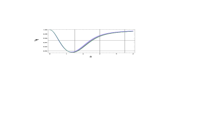
Figure 1: Fidelity as a function of $\delta=\gamma J$, for different values of $J$, ($J=10,...100)$. For large $J$ the curves become virtually indistinguishable.

Now we return to the discussion of the spectral gap in our system.

III.2 Variational upper bound for the gap

Having discussed the exactness of our trial vector (13), we now compare the expectation value of the energy $\Delta E_{0}=\left\langle\Phi_{0}\right|H\left|\Phi_{0}\right\rangle$ of the state (13) to the exact excited state energy by calculating the ratio $\Delta E/\Delta E_{0}$. To express $\left\langle\Phi_{0}\right|H\left|\Phi_{0}\right\rangle$ in suitable form we use the identity

$$\left[\exp\left(-\gamma J_{y}\right)\right]_{m,m^{\prime}}=d_{m^{\prime},m}^{J}\left(i\gamma\right),$$ (19)

where $d_{m^{\prime},m}^{J}\left(x\right)$ is the Wigner rotation matrix, familiar from the quantum mechanics biedenharn . After a lengthy but straightforward calculation we eventually obtain the following expression

$$\Delta E_{0}=\Omega_{0}^{2}\left(\cosh 2\gamma+\left(J+2\right)\frac{P_{J-2}^{1,3}\left(\cosh 2\gamma\right)\sinh\gamma\cosh^{3}\gamma+P_{J+2}^{-3,-1}\left(\cosh 2\gamma\right)\sinh^{-3}\gamma\cosh^{-1}\left(\gamma\right)}{P_{J-1}^{0,2}\left(\cosh 2\gamma\right)\cosh^{2}\gamma+P_{J-1}^{2,0}\left(\cosh 2\gamma\right)\sinh^{2}\gamma}\sinh 2\gamma\right),$$ (20)

where $P_{n}^{\alpha,\beta}\left(x\right)$ are Jacobi polynomials Szego .

To illustrate that the upper bound $\Delta E_{0}$ can be considered as an accurate estimation of the gap, we have numerically calculated the first excited state energy $\Delta E$ of the Hamiltonian. In Fig. 2 we have plotted $\Delta E/\Delta E_{0}$ as a function of $\delta$ for for different values of $J$ up to $100$.

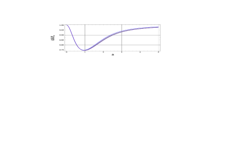
Figure 2: Energy of first excited states  as a function of $\delta=\gamma J$ with respect to the variational bound (20) for different $J$.

As we see from Fig.2 the behavior of $\Delta E/\Delta E_{0}$ is very similar to the fidelity $\mathcal{F}$. For sufficiently large values of $J$   and $\gamma\neq 0$, one can easily obtain a simple expression for $\Delta E_{0}$. Making use of the asymptotics of the Jacobi polynomials for large $J$, namely Szego ,

$$P_{J}^{\alpha,\beta}\left(x\right)\approx\frac{\left(x^{2}-1\right)^{-1/4}}{\sqrt{2\pi J}}\left[x+\left(x^{2}-1\right)^{1/2}\right]^{J+1/2}\left(x-1\right)^{-\alpha/2}\left(x+1\right)^{-\beta/2}\left[\left(x+1\right)^{1/2}+\left(x-1\right)^{1/2}\right]^{\alpha+\beta},x>1$$ (21)

one arrives at the simple expression

$$\Delta E_{0}\approx\Omega_{0}^{2}\left(\cosh 2\gamma+J\sinh 2\gamma\right).$$ (22)

Thus, we see $\Delta E_{0}$ grows linearly as $J>>1$ for all $\gamma>0$. A better result for $\Delta E$ at intermediate values $\delta$ can be obtained with the state $\left|+\right\rangle$. Substituting of the state vector $\left|+\right\rangle$ in the formula (11), we obtain

$$\Delta E_{+}=\frac{\left\langle+\right|H\left|+\right\rangle}{1-\left|\left\langle+\right|\left.\Phi_{g}\right\rangle\right|^{2}}=\Omega_{0}^{2}\frac{\cosh^{2}\gamma+\dfrac{\left(J+2\right)\left(J-1\right)}{4}\sinh^{2}\gamma}{1-\frac{2J}{J+1}\dfrac{P_{J}^{1,-1}\left(\cosh\gamma\right)}{P_{J}\left(\cosh 2\gamma\right)}}$$ (23)

Combining this expression with formula (20), we can derive an upper bound for

$$\Delta E\leq\Omega_{0}^{2}\min\left[\Delta E_{0},\Delta E_{+}\right].$$ (24)

For a state composed of $\left|\Phi_{0}\right\rangle$ and $\left|+\right\rangle$ states i.e. the state (17) the minimum of

$$\Delta E_{V}\left(\eta\right)=\frac{\left\langle\Phi_{V}\left(\eta\right)\right|H\left|\Phi_{V}\left(\eta\right)\right\rangle}{\left\langle\Phi_{V}\left(\eta\right)\right|\left.\Phi_{V}\left(\eta\right)\right\rangle-\left|\left\langle\Phi_{V}\left(\eta\right)\right|\left.\Phi_{g}\right\rangle\right|^{2}}$$

would be better than (24). We do not explicitly give this lengthy optimal bound, but rather present in Fig.3 the minimum of $\Delta E_{V}\left(\eta\right)/\Delta E$ (see Fig.3a) and $\min\left[\Delta E_{0},\Delta E_{+}\right]/\Delta E$ as function of $\delta$.

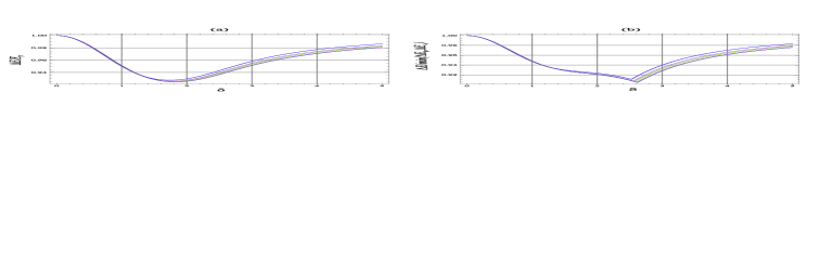
Figure 3: Energy of first excited states  as a function of $\delta=\gamma J$ with resprct to the variational bounds obtained by minimization of $\Delta E_{V}\left(\eta\right)$ (a) and $\min\left(\Delta E_{0},\Delta E_{+}\right)$ (b) for different $J$ (from $10$ to $100$).

As we can see from Fig.3(a), the variational state (17) which depends on the single parameter $\eta$, accurately recovers the true excited state energy within $0.8\%$.  The accuracy of the relatively simple upper bound (24) ( see Fig.3(b)) is a few percent less than the optimal bound given by (17). It is a remarkable result considering the simplicity of the trial function used. Thus, we have seen that at a quantitative level the variational upper bounds for the gap are in a good agreement with exact numerical results (for $J$ up $100$). But these observations do not provide a rigorous proof that the system is indeed gapped. So the problem is to get a non trivial lower bound for $\Delta E$. Next we turn our attention to this issue.

IV Lower bound for the spectral gap

We now turn to the problem of obtaining a non trivial lower bound for the gap by a suitable choice of the form of the Hamiltonian. To this end, we need some facts from the theory of matrices. For notation simplicity, throughout this section we denote by $\lambda_{n}\left(X\right)$ $\left(n=1,2,...M\right)$ eigenvalues of a $M\times M$ Hermitian matrix $X$ in increasing order, i.e. $\left\{\lambda_{1}\left(X\right)\geq\lambda_{2}\left(X\right)\geq...\geq\lambda_{M}\left(X\right)\right\}$.  A lower bound for the spectral gap can be obtained using the Weyl’s theorem Weyl which is stated as follows. Let $X$, $Y$  and $Z$ with $Z=X+Y$ be $M$-dimensional Hermitian matrices, then

$$\lambda_{i+j-1}\left(Z\right)\leq\lambda_{i}\left(X\right)+\lambda_{j}\left(Y\right),$$ (25)

whenever $i+j-1\leq M$, or equivalently

$$\lambda_{k}\left(Z\right)\geq\lambda_{i}\left(X\right)+\lambda_{j}\left(Y\right),$$ (26)

if $i+j=M+k$.

To apply the Weyl’s theorem we split the Hamiltonian (12) into two parts:

$$H=H_{X}+\Omega_{0}^{2}J_{z}^{2},$$ (27)

where

$$H_{X}=\Omega_{0}^{2}\left(\left(J_{z}^{2}+J_{y}^{2}\right)\sinh^{2}\gamma-J_{x}\sinh\gamma\cosh\gamma\right)=$$

$$=\Omega_{0}^{2}\left(\left(J(J+1)-J_{x}^{2}\right)\sinh^{2}\gamma-J_{x}\sinh\gamma\cosh\gamma\right).$$ (28)

In the second line we have used the identity $J_{z}^{2}+J_{y}^{2}+J_{x}^{2}=J(J+1)$. Using the inequality (26) and recalling supersymmetric property of our Hamiltonian for the spectral gap, i.e. $\Delta E=\lambda_{2J}\left(H\right)=\lambda_{2J-1}\left(H\right)$, one obtains

$$\Delta E/\Omega_{0}^{2}\geq\lambda_{i}\left[\left(J(J+1)-J_{x}^{2}\right)\sinh^{2}\gamma-J_{x}\sinh\gamma\cosh\gamma\right]+\lambda_{j}\left(J_{z}^{2}\right),$$ (29)

where $i+j=4J$. It is not hard to verify directly that the possible pairs of $\left(i,j\right)$ are $\left(2J+1,2J-1\right),$ $\left(2J-1,2J+1\right),$ and $(2J,2J)$. The corresponding energies are

$$E_{ge}/\Omega_{0}^{2}=1-J\exp\left(\gamma\right)\cdot\sinh\gamma\rightarrow\left(2J+1,2J-1\right),$$ (30)

$$E_{eg}/\Omega_{0}^{2}=\min\left[J\cdot\mathtt{\exp}\left(\gamma\right)\cdot\sinh\gamma,\left(5J-4\right)\sinh^{2}\gamma-\frac{1}{2}\left(J-2\right)\sinh 2\gamma\right]\rightarrow\left(2J-1,2J+1\right),$$ (31)

$$E_{ee}/\Omega_{0}^{2}=1+\left(3J-1\right)\sinh^{2}\gamma-\frac{1}{2}\left(J-1\right)\sinh 2\gamma\rightarrow\left(2J,2J\right)$$ (32)

The bound (30) is a trivial one, it goes to negative values as $\gamma$ becomes large $\gamma>\ln\left(1+2/J\right)\approx 2/J$. For small $\gamma<<1/J$ , the bound (32) is better than (31) and it becomes negative for $1/J\lesssim\gamma\lesssim 0.3$. While, for relatively large $\gamma\gtrsim 0.2$ the bound (31) is much better than (32), although it becomes negative when $\gamma\lesssim 0.2$. Hence, on the basis of these analyses we arrive at the inequality for

$$\Delta E\geq\Omega_{0}^{2}\min\left[J\cdot\mathtt{\exp}\left(\gamma\right)\cdot\sinh\gamma,\text{ }\left(5J-4\right)\sinh^{2}\gamma-\frac{1}{2}\left(J-2\right)\sinh 2\gamma\right],$$ (33)

which gives a trivial bound for $\gamma\lesssim 0.2$ but a nontrivial one for large $\gamma$. By comparing (22) and (33) for large $\gamma$ and $J$ we conclude that the upper and lower bounds on $\Delta E$  converge to each other. Hence, it remains  to be found a non trivial lower bound for intermediate values of $\gamma$.

In the following we show that by using the representation (7) the degeneracy and a non trivial lower bound (for arbitrary $\gamma$ and integer $J$), for $\Delta E$ can be obtained through direct calculations.

It is easily seen that the Hamiltonian (7) is similar to the non-Hermitian Hamiltonian

$$H_{\mathtt{n}}=\exp\left(-\gamma J_{x}\right)H\exp\left(\gamma J_{x}\right)=\Omega_{0}^{2}\exp\left(-2\gamma J_{x}\right)J_{z}\exp\left(2\gamma J_{x}\right)J_{z}=$$

$$=\Omega_{0}^{2}\left(J_{z}^{2}\cosh 2\gamma+iJ_{y}J_{z}\sinh 2\gamma\right).$$ (34)

We show that, beside its non-Hermiticity the spectral properties of (34) are very transparent. Indeed, from Eq. (34), one can see clearly first that it has a null state $\left|m_{z}=0\right\rangle$ ( $J_{z}\left|m_{z}=0\right\rangle=0$ ). Second, all excited states are two-fold degenerate. To see this, we notice that $H_{\mathtt{n}}$ can be represented as a block matrix

$$H_{\mathtt{n}}=\left(\begin{array}[c]{ccc}\underset{J\times J}{\underbrace{H_{-}}}&\underset{1\times J}{\underbrace{0}}&\underset{J\times J}{\underbrace{0}}\\ \left\langle a\right|&0&\left\langle b\right|\\ \underset{J\times J}{\underbrace{0}}&\underset{1\times J}{\underbrace{0}}&\underset{J\times J}{\underbrace{H_{+}}}\end{array}\right),$$ (35)

in the eigenbasis of $J_{z}$. $H_{+}$ and $H_{-}$ are real permutation equivalent matrices, i.e. they have the same spectrum. The transposed vectors $\left\langle a\right|$ and $\left\langle b\right|$ connect the state $\left|m_{z}=0\right\rangle$ with negative and positive magnetic quantum numbers $m_{z}$.

As an example, consider $J=2$, the Hamiltonian $H_{\mathtt{n}}$ , has the following form

$$H_{\mathtt{n}}=\Omega_{0}^{2}\left(\begin{array}[c]{ccccc}4\cosh 2\gamma&\sinh 2\gamma&0&0&0\\ -2\sinh 2\gamma&\cosh 2\gamma&0&0&0\\ 0&-\frac{\sqrt{6}}{2}\sinh 2\gamma&0&-\frac{\sqrt{6}}{2}\sinh 2\gamma&0\\ 0&0&0&\cosh 2\gamma&-2\sinh 2\gamma\\ 0&0&0&\sinh 2\gamma&4\cosh 2\gamma\end{array}\right),$$

where

$$H_{-}=\Omega_{0}^{2}\left(\begin{array}[c]{cc}4\cosh 2\gamma&\sinh 2\gamma\\ -2\sinh 2\gamma&\cosh 2\gamma\end{array}\right),\text{ \ }H_{+}=\Omega_{0}^{2}\left(\begin{array}[c]{cc}\cosh 2\gamma&-2\sinh 2\gamma\\ \sinh 2\gamma&4\cosh 2\gamma\end{array}\right)$$

and

$$\left\langle a\right|=\Omega_{0}^{2}\left(0,-\frac{\sqrt{6}}{2}\sinh 2\gamma\right),\text{ }\left\langle b\right|=\Omega_{0}^{2}\left(-\frac{\sqrt{6}}{2}\sinh 2\gamma,0\right).$$

One can see that $H_{+}$ and $H_{-}$ are permutation equivalent, i.e.

$$H_{-}=\left(\begin{array}[c]{cc}0&1\\ 1&0\end{array}\right)H_{+}\left(\begin{array}[c]{cc}0&1\\ 1&0\end{array}\right).$$

The matrix elements of $H_{+}$  are

$$\left(H_{+}\right)_{m,m^{\prime}} =\Omega_{0}^{2}\left(m^{2}\delta_{mm^{\prime}}\cosh\left(2\gamma\right)+\frac{m^{\prime}}{2}\sinh 2\gamma\left[\delta_{m,m^{\prime}+1}\sqrt{\left(J-m^{\prime}\right)\left(J+m^{\prime}+1\right)}-\delta_{m,m^{\prime}-1}\sqrt{\left(J+m^{\prime}\right)\left(J-m^{\prime}+1\right)}\right]\right)$$ (36)

$$m,m^{\prime} =J,J-1,...,1.$$

The spectrum of $H_{\mathtt{n}}$ can be obtained from the following algebraic equation

$$\lambda\det\left(\lambda\cdot{{1\!\!1}}_{J\times J}-H_{+}\right)\det\left(\lambda\cdot{{1\!\!1}}_{J\times J}-H_{-}\right)=0.$$ (37)

Since $H_{+}$ and $H_{-}$ have the same spectrum, the spectrum of $H_{\text{n}}$ is doubly degenerate except for the eigenstate $\left|m_{z}=0\right\rangle$.  Therefore, we may restrict ourselves to the study of spectral properties of $H_{+}$. We thus have verified directly that for integer $J$ and for arbitrary $\gamma$ the spectrum of the initial Hamiltonian (7) is supersymmetric. And, in addition to that the excited spectrum of the Hamiltonian (7) coincides with the spectrum $H_{+}$ i.e. the spectral gap of our model coincides with the ground state energy of $H_{+}$.

As one can see from Eq (36), the matrix $H_{+}$ can be represented in a compact form

$$H_{+}=\Omega_{0}^{2}\left(j_{z}^{2}\cosh 2\gamma+i\cdot j_{y}\cdot j_{z}\sinh 2\gamma\right),$$ (38)

where the truncated Hermitian angular momentum matrices $j_{z}$ , $j_{y}$ and $j_{x}$ satisfy the following commutation relations

$$\left[j_{z},j_{x}\right] =ij_{y},$$ (39)

$$\left[j_{y},j_{z}\right] =ij_{x},$$

but unlike the ordinary angular momentum operators

$$\left[j_{x},j_{y}\right]\neq ij_{z}.$$ (40)

Next, we will show that the Hamiltonian $H_{+}$ can be transformed into a more pleasant form. To this end, we recall that $j_{z}$ is a positive definite matrix with eigenvalues $1,2,...J$. So that the square root $j_{z}^{1/2}$is well defined. Using this, the matrix $H_{+}$ can be written as

$$H_{+}=j_{z}^{-1/2}\cdot h\cdot j_{z}^{1/2},$$ (41)

where

$$h=\Omega_{0}^{2}\left(j_{z}^{2}\cosh 2\gamma+i\cdot j_{z}^{1/2}\cdot j_{y}\cdot j_{z}^{1/2}\sinh 2\gamma\right)$$ (42)

which has the same spectrum as $H_{+}$. Now we state that for any $\gamma$ and $J$

$$\Delta E\geq\Omega_{0}^{2}\cosh 2\gamma.$$ (43)

Indeed, for any eigenvalue $E\left(h\right)>0$ of $h$ and its corresponding normalized eigenvector $\left|\varphi\right\rangle$ we have

$$E\left(h\right)=\left\langle\varphi\right|h\left|\varphi\right\rangle=$$

$$=\Omega_{0}^{2}\left(\left\langle\varphi\right|j_{z}^{2}\left|\varphi\right\rangle\cosh 2\gamma+i\left\langle\varphi\right|j_{z}^{1/2}\cdot j_{y}\cdot j_{z}^{1/2}\left|\varphi\right\rangle\sinh 2\gamma\right)=$$

$$=\Omega_{0}^{2}\left\langle\varphi\right|j_{z}^{2}\left|\varphi\right\rangle\cosh 2\gamma\geq$$

$$\geq\Omega_{0}^{2}\cosh 2\gamma$$

where in the second line we have used the fact that $j_{z}^{1/2}\cdot j_{y}\cdot j_{z}^{1/2}$ is a Hermitian matrix. In the last line we have used the fact that the smallest eigenvalue of $j_{z}$ is equal $1$. Hence, all eigenvalues of $h$ lie at finite distances from the origin greater than $\cosh 2\gamma$ i.e. the spectral gap of the antiferromagnetic SUSY LMG Hamiltonian (7) is bounded from below by $\Omega_{0}^{2}\cosh 2\gamma$. Unlike the inequality (33), it does not involve $J$.

V Discussion and Conclusion

In the present paper we have investigated the spectrum of the antiferromagnetic LMG model at the SUSY point. We have proved, by explicitly constructing the supercharges, that the Hamiltonian (1) is supersymmetric at $\lambda=1$. By using the explicit form  of the ground state of the Hamiltonian we have introduced variational excited states that have pretty high fidelity with the exact excited state. A simple form of these states enables us to find closed expressions for upper bounds for the spectral gap. It was shown numerically that the obtained upper bounds are in good agreement with the exact spectral gap. Simple but non trivial lower bounds for the spectral gap was found. Thus, we have shown that the antiferromagnetic SUSY LMG model is gapped for any values of $\gamma$. Although, for intermediate values of $\gamma$ the obtained lower bound

$$\Delta E\geq\Omega_{0}^{2}\max\left[\cosh 2\gamma,\min\left[J\cdot\mathtt{\exp}\left(\gamma\right)\cdot\sinh\gamma,\text{ }\left(5J-4\right)\sinh^{2}\gamma-\frac{1}{2}\left(J-2\right)\sinh 2\gamma\right]\right]$$

is not tighter than those of variational bounds, it can be used for studies of low-energy physics in the LMG model e.g. for estimating the duration of the adiabatic quantum processes in ionic traps Blatt . There is no doubt that it is possible to improve this lower bound. We hope to come back to these topics in a future publication.

I am grateful to M. Fleischhauer for many fruitful and stimulating discussions.

References

(1)H. J. Lipkin, N. Meshkov, and A. J. Glick, Nucl. Phys.
62, 188 (1965); N. Meshkov, A. J. Glick, and H. J. Lipkin, Nucl.
Phys. 62, 199 (1965); A. J. Glick, H. J. Lipkin, and N. Meshkov,
Nucl. Phys. 62, 211 (1965).
(2)J. I. Cirac, M. Lewenstein, K. Mølmer, and P. Zoller, Phys.
Rev. A 57, 1208 (1998).
(3)R.G. Unanyan, M. Fleischhauer, Phys. Rev. Lett.,
90, 133601 (2003); R. G. Unanyan, C. Ionescu, M. Fleischhauer, Phys.
Rev. A 72, 022326 (2005).
(5)E. Witten, Nucl. Phys. B 188, 513 (1981); L. E.
Gendenshtein and I. V. Krive, Usp. Fiz. Nauk 146, 553 (1985); F.
Cooper, A. Khare and U. Sukhatme, Phys. Rep. 267, 267 (1995).
(6)C. Eckert, Phys. Rev. 36, 878 (1930).
(7)A. Garg, Phys. Rev. B, 64, 094413 (2001); E.
Kececioglu and A. Garg, Phys. Rev. Lett. 88 , 237205 (2002).
(8)L. Biedenharn and J. D. Louck , Angular
Momentum in Quantum Physics Theory and Application, Addison-Wesley 1981;
D.A. Varshalovich, A.N. Moskalev, V.K. Kheronskii, Quantum
theory of Angular Momentum,World Scientific, 1988.
(9)G. Szegö, Orthogonal Polynomials, American Mathematical
Society, Colloquium Publications, vol. 23, New York 1939.
(10)H. Weyl, Math. Ann. 71, 441 (1912); W. Fulton,
Bull. Amer. Math. Soc., 37: 209 (2000).
(11)R. Blatt and C. F. Roos, Nature Physics 8, 277 (2012).