Collective Modes in the Superfluid Inner Crust of Neutron Stars

Abstract

The neutron-star inner crust is assumed to be superfluid at relevant temperatures. The contribution of neutron quasiparticles to thermodynamic and transport properties of the crust is therefore strongly suppressed by the pairing gap. Nevertheless, the neutron gas still has low-energy excitations, namely long-wavelength collective modes. We summarize different approaches to describe the collective modes in the crystalline phases of the inner crust and present an improved model for the description of the collective modes in the pasta phases within superfluid hydrodynamics.

26.60.Gj

1 Introduction

A neutron star has a very dense core, consisting probably of homogeneous and very neutron-rich matter (other constituents are protons, electrons, and perhaps hyperons; the extremely dense center of the core might even contain deconfined quark matter), which is surrounded by the inner and the outer crust.[1] In the crust, the baryon density $n_{B}$ is below $\sim 0.08$ fm^-3 (i.e., mass density $\varrho\lesssim 1.3\times 10^{14}$ g$/$cm³) and the matter is inhomogeneous, containing dense positively charged “clusters” and a highly degenerate electron gas. The difference between the inner and the outer crust is that in the outer crust, the clusters are simply neutron-rich nuclei, while in the inner crust (at mass density $\varrho\gtrsim 4\times 10^{11}$ g$/$cm³,[1] i.e., baryon density $n_{B}\gtrsim 2.4\times 10^{-4}$ fm^-3), the neutron excess becomes so strong that some neutrons are not bound any more in the clusters and form a dilute neutron gas between the clusters.[2] To minimize Coulomb energy, the clusters are believed to arrange in a periodic lattice. With increasing density of the neutron gas near the core, the crystalline lattice might transform into the so-called “pasta” phases, i.e., clusters merge first into rods (“spaghetti”), then into plates (“lasagne”), and then some theories predict also “inverted” geometries where the more dilute neutron gas is concentrated in tubes or holes (“Swiss cheese”) before the homogeneous core is reached.[3, 4]

In the first 50–100 years after the creation of the neutron star in a supernova explosion, its core cools down very efficiently by neutrino emission. During this so-called crust-thermalization epoch, the crust stays hotter than the core. Since the observed temperature is that at the surface, the thermal properties of the crust influence the observed cooling curve.[5] In accreting neutron stars, the matter falling on the star results from time to time in nuclear reactions in the crust, leading to a strong heating (released as X-ray burst). The subsequent cooling of these X-ray transients offers another possibility to get information on the thermodynamic properties of the crust.[6, 7]

The main ingredients to describe heat transport in the crust are the specific heat and the heat conductivity. They depend mainly on excitations whose energy is of the same order of magnitude as the temperature $T$. Since on a nuclear energy scale, the temperatures of interest ($10-100$ keV, corresponding to $10^{8}-10^{9}$ K) are very low, the most relevant excitations in the outer crust are the electrons (specific heat $c_{v}\propto T$) and the phonons of the crystal lattice ($c_{v}\propto T^{3}$). In the inner crust, the situation is more complicated, since there are in addition the unbound neutrons of the gas between the clusters. If these neutrons were a normal Fermi gas, their contribution to $c_{v}$ at low $T$ would be linear in $T$, like that of the electrons but much larger due to the higher density of states. However, for most of the relevant densities and temperatures one can assume that the neutrons are superfluid (although the density dependence of the critical temperature $T_{c}$ of neutron matter is not precisely known). In this case, the energy for the creation of a neutron quasiparticle is of the order of the pairing gap $\Delta\sim 1$ MeV, and analogously to the specific heat of a superconductor,[8] the contribution of neutron quasiparticles to the specific heat is exponentially suppressed ($\propto e^{-\Delta/T}$) at low $T$. It was therefore argued that whether neutron pairing is stronger or weaker can have an observable effect on the cooling curve.[6, 9] Vice versa, observation of neutron-star cooling might help to constrain the superfluid critical temperature in neutron star matter.[10, 11]

In contrast to the gapped neutron quasiparticles, long-wavelength collective modes of the neutron gas can be thermally excited at low temperature and contribute to the specific heat and the heat conductivity (although the electron and lattice-phonon contributions are usually dominant[41]).

This article is divided into two parts. In Sec. 2, we start by discussing collective modes in homogeneous low-density neutron matter and in particular the appearance of the Goldstone mode as a phase oscillation of the superfluid order parameter (gap) and its connection with superfluid hydrodynamics. For inhomogeneous crust matter, we then summarize results of completely microscopic calculations, which are however limited to wavelengths smaller than the distance between neighboring clusters, as well as results in the long-wavelength limit. In Sec. 3, we discuss in detail a model for collective modes in the pasta phases, in particular in the lasagne phase, based on superfluid hydrodynamics.

Throughout the article, we use natural units with $\hbar=c=k_{B}=1$ ($\hbar=$ reduced Planck constant, $c=$ speed of light, $k_{B}=$ Boltzmann constant).

2 QRPA, Goldstone Mode, and Superfluid Hydrodynamics

2.1 QRPA in uniform neutron matter

For simplicity, let us start our discussion with a uniform neutron gas, although this is of course a very incomplete model of the inner crust since it neglects the presence of dense clusters.

Collective modes are conveniently described in the framework of the Random-Phase Approximation (RPA) for the response of uniform matter.[12, 13] It has already been used in astrophysical contexts, e.g., to calculate the neutrino mean-free path.[14] However, the RPA does not include pairing and superfluidity. The extension of the RPA to systems with pairing is called Quasiparticle RPA (QRPA).[15] QRPA calculations in uniform neutron and neutron-star matter, using the so-called Landau approximation for the particle-hole (ph) interaction, were done in Refs. 16, 17. Here we will discuss results for neutron matter obtained in Ref. 18 with the full Skyrme interaction in the ph channel. Also in other fields of physics, the RPA was generalized to systems with pairing. Let us mention the seminal work by Anderson[19] and Bogoliubov[20] for the case of superconductors, or some more recent work on collective modes in ultracold Fermi gases in the unitary limit.[21, 22]

The QRPA describes small oscillations around the Hartree-Fock-Bogoliubov (HFB) ground state and can be derived by linearizing the time-dependent HFB equations.[15] In the left panel of Fig. 1,

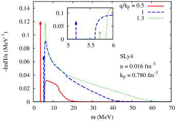
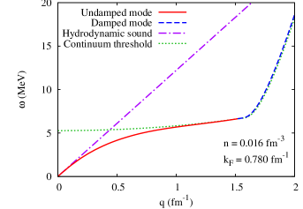
Figure 1: Left panel: QRPA results of Ref. 18 for the density response $\Pi$ for neutron matter with density $n=0.016$ fm^-3. The imaginary part of $\Pi(\omega,q)$ is shown as function of the excitation energy $\omega$ for three different values of $q$. The arrows represent $\delta$-functions corresponding to the undamped collective mode. Right panel: Dispersion relation of the collective mode obtained within QRPA (solid and dashed lines) and the linear dispersion relation of hydrodynamic sound (dash-dotted line). The 2qp threshold${}^{\ref{footnote:gmb}}$ is indicated by the dots.

we show the QRPA density response function $\Pi(\omega,q)$ of neutron matter, as a function of the excitation energy $\omega$ for different values of the momentum $q$. At first glance, the response resembles the broad ph continuum of the usual RPA response. Since the Landau parameter $F_{0}$ relevant for the density channel is negative, there is no zero-sound above the continuum.[23] However, at low energies, one sees that, because of pairing, the ph continuum starting at $\omega=0$ is transformed into a two-quasiparticle (2qp) continuum starting at a threshold given by approximately $2\Delta$. This gives rise to the appearance of an undamped collective mode below the threshold, indicated by the arrows.

The nature of this collective mode is a phase oscillation of the gap $\Delta=|\Delta|e^{i\phi}$. In the ground state, the phase $\phi$ is arbitrary but constant (spontaneous $U(1)$ symmetry breaking). Usually it is assumed without loss of generality that $\Delta$ is real, i.e., $\phi=0$, but a global change of the phase does not cost any energy. However, if the phase varies spatially as $\phi\propto e^{i\bm{\mathrm{q}}\cdot\bm{\mathrm{r}}}$, the excitation energy $\omega$ is proportional to $q$. Such a mode related to a spontaneously broken symmetry is called a Goldstone mode,[26, 27] in the case of a superfluid it is also known as Bogoliubov-Anderson (BA) sound. Note that this BA sound[19, 20] exists only in superfluids but not in superconductors: In the case of charged particles, the broken symmetry is a local one (the electromagnetic gauge symmetry) and in this case there is no Goldstone mode.[27]

If the phase $\phi(\bm{\mathrm{r}})$ is not constant, the Cooper pairs (of mass $2m_{n}$, where $m_{n}$ denotes the neutron mass) move with a collective velocity[28]

$$\bm{\mathrm{v}}=\frac{1}{2m_{n}}\bm{\mathrm{\nabla}}\phi\,.$$ (1)

Hence, the Goldstone mode corresponds to a longitudinal density wave. In contrast to zero sound, the Goldstone mode does not deform the Fermi sphere during the oscillation. Therefore its speed of sound $u$ is given by the hydrodynamic formula

$$u^{2}=\frac{n_{n}}{m_{n}}\frac{\partial\mu_{n}}{\partial n_{n}}\,,$$ (2)

where $\mu_{n}$ and $n_{n}$ are the neutron chemical potential and density, respectively.

In the right panel of Fig. 1, we show the dispersion relation $\omega(q)$ (solid line) of the collective mode obtained in QRPA. As anticipated, it agrees perfectly with the hydrodynamic one $\omega=uq$ for small $q$ (dash-dot line). However, when $\omega$ approaches the 2qp theshold (dotted line), it deviates from the linear dispersion law. At high values of $q$, the collective mode enters the 2qp continuum and gets damped (dashed line).

At low temperatures $T\ll\Delta$, one may neglect the temperature dependence of the dispersion relation and the damping of the Goldstone mode. Since mainly modes with $\omega\sim T$ are excited, the deviations from the linear dispersion law $\omega=uq$ are negligible, too. Therefore, the neutron-gas contribution to the specific heat at low temperature can be written analytically as

$$c_{v,{\mathit{coll}}}=\frac{2\pi^{2}T^{3}}{15\,u^{3}}$$ (3)

analogous to the specific heat of phonons in a crystal.[29, 30] On the one hand, this is of course much larger than the contribution of neutron quasiparticles, which is suppressed by an exponential factor $e^{-\Delta/T}$. On the other hand, it is still much smaller than the specific heat of normal-fluid (i.e., unpaired) neutrons, which would be linear in $T$.

2.2 QRPA in a Wigner-Seitz cell

So far, we have discussed only a homogeneous neutron gas. In order to describe clusters in the gas, often the Wigner-Seitz (WS) approximation is employed. This approximation consists in replacing the elementary cell of the crystal lattice by a sphere of radius $R_{{\mathit{WS}}}$, having the same volume as the elementary cell, with the cluster in its center. The advantage is that then all quantities, i.e., the densities, the mean-field, the Coulomb potential, etc., depend only on the distance $r$ from the center of the cell. This spherical symmetry makes it possible to carry out HF[2] or HFB[31, 32] calculations with the large numbers of particles contained in a WS cell. As an example, we display in the left panel of Fig. 2

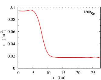
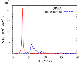
Figure 2: Left panel: HFB density profile calculated by Khan et al.[32] in a WS cell with $R_{{\mathit{WS}}}=27.6$ fm, containing 1750 neutrons and 50 protons (¹⁸⁰⁰Sn). Right panel: quadrupole response of neutrons in the same WS cell calculated by Khan et al.[32] within the QRPA (solid line; for comparison, the dashed line shows the unperturbed HFB quasiparticle response) as function of the excitation energy $\omega$.

the HFB density profile in a WS cell containing 1750 neutrons and 50 protons (¹⁸⁰⁰Sn) calculated by Khan et al.[32] The nuclear cluster surrounded by the gas is clearly visible, the gas density being practically constant for $r\gtrsim 12$ fm (except for a small bump near $R_{{\mathit{WS}}}$ which is an artefact due to the boundary conditions[2, 31]).

Based on the HFB ground state, Khan et al.[32] calculated the collective modes within QRPA, too. As an example, the right panel of Fig. 2 shows the quadrupole strength (imaginary part of the quadrupole response function) within the WS cell as a function of the excitation energy $\omega$. A strongly collective mode, called “super-giant resonance” in Ref. 32, appears well below the unperturbed 2qp quadrupole excitations (dotted line).

This super-giant resonance is mainly an excitation of the neutron gas. Its energy of $\sim 3$ MeV as can be seen in Fig. 2 can be roughly understood by considering it as the lowest eigenmode of the hydrodynamic (BA) sound in the spherical cell. In Ref. 32, this energy was estimated as $\omega=v_{F}q/\sqrt{3}$ ($v_{F}$ being the Fermi velocity) with $q$ determined from $j_{l}(qR_{{\mathit{WS}}})=0$ ($j_{l}$ being a spherical Bessel function; in the case of the quadrupole mode: $l=2$). Note, however, that $v_{F}/\sqrt{3}$ is the speed of sound of an ideal Fermi gas, which is about 50% higher than the speed of sound $u$ one gets from Eq. (2).

The argument for the (approximate) validity of hydrodynamics is that the WS cell is much larger than the coherence length $\xi$ in the neutron gas.[32] Actually, up to some factors of order unity, the condition $\xi\ll R_{{\mathit{WS}}}$ or $\xi q\ll 1$ is equivalent to $\omega\ll\Delta$. Obviously these conditions are not very well satisfied, so that one expects to find at a quantitative level some deviations from hydrodynamics, similar to the deviation of the QRPA dispersion relation $\omega(q)$ in uniform matter from the linear one, $\omega=uq$ (cf. Fig. 1).

Let us mention that the correspondence between QRPA and superfluid hydrodynamics in non-uniform systems in the case of strong enough pairing was demonstrated in Ref. 33 in the context of trapped ultracold Fermi gases, too. However, because of the typically very large numbers of atoms and strong pairing in these systems, the situation is usually much more favorable than it is in the neutron star crust, and superfluid hydrodynamics can give precise predictions for the frequencies of collective modes.[34]

2.3 Low-energy theory for large wavelengths

While the WS approximation is well suited for the description of static properties, it is obviously not capable of describing collective modes whose wavelengths exceed the size of the WS cell. In reality, however, the most relevant modes at low temperature are acoustic modes, i.e., modes whose energy $\omega$ is proportional to $q$ for $q\ll 1/R_{{\mathit{WS}}}$.

As mentioned in Sec. 2.1, the Goldstone mode in the uniform neutron gas is a consequence of the broken global $U(1)$ symmetry and corresponds to an oscillation of the phase $\phi$ of the neutron gap. This argument remains valid in the presence of clusters. This lead Cirigilano et al.[38] to develop an effective theory for the combined system of the superfluid neutron gas and the crystal lattice of clusters. The degrees of freedom, i.e., the fields appearing in the effective Lagrangian, are the phase $\phi(\bm{\mathrm{r}},t)$ of the neutron gap and the displacement $\bm{\xi}(\bm{\mathrm{r}},t)$ of the clusters. Similar low-energy theories were subsequently used in Refs. 39, 40. Since $\phi$ and $\bm{\xi}$ are coarse-grained over regions larger than the periodicity $L$ of the crystal lattice, these low-energy theories are only valid for $q\ll 1/L$.

Of course, clusters and neutron superfluid do not move independently of each other. This is called the entrainment effect.[35] It should be noted that in contrast to an ordinary dragging of the gas by the clusters (and vice versa), the entrainment is a non-dissipative force. It modifies the velocities $u_{l}$ and $u_{t}$ of the longitudinal and transverse lattice phonons, respectively, as well as the velocity $u_{\phi}$ of the Goldstone mode (also called superfluid phonon).[39] Furthermore, the longitudinal lattice phonons and the Goldstone mode get mixed[38, 39, 40] and one finds two new eigenmodes with two new velocities $u_{\pm}$. The framework of low-energy effective theory was not only used to describe the long-wavelength phonons, but also phonon-phonon and phonon-electron interactions. These are particularly relevant for the calculation of the phonon (lattice and superfluid) contribution to transport properties such as the heat conductivity.[41]

The coefficients of the effective theory, in particular the entrainment and mixing coefficients, were calculated by Chamel[37] using a band-structure calculation for the neutrons in the periodic mean field of the clusters[36] analogous to those used in solid-state physics for the electrons in the periodic Coulomb field of the ions in a metal. As an example, we display in Fig. 3

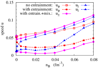
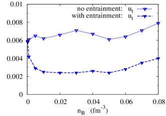
Figure 3: Velocities of the longitudinal and superfluid phonons ($u_{l}$ and $u_{\phi}$, left panel) and of the transverse phonons ($u_{t}$, right panel) as a function of the baryon density $n_{B}$, from Chamel et al.[39] Dotted lines: entrainment neglected; dashed lines: entrainment included; solid lines: entrainment and mixing included.

the results of Ref. 39 for the density dependence of the different velocities without (dotted lines) and with (dashed lines) entrainment and with both entrainment and mixing (solid lines). One observes that the coupling between the lattice and the superfluid neutron gas has a drastic effect on the lattice phonons. The entrainment results in a reduction of the phonon velocities, since some neutrons of the gas move together with the clusters, increasing the cluster effective mass (in the language of Refs. 37, 39, the density of “conduction neutrons” moving independently of the clusters is smaller than the density of “unbound” neutrons).

However, as pointed out by Kobyakov and Pethick,[40] zero-point oscillations of the clusters may reduce the band structure effects. Furthermore, we note that, using a completely different approach (similar to the one we will use in the next section), Magierski and Bulgac[43, 44] arrived at the opposite result, namely that the effective mass of the clusters is reduced when they are immersed in the neutron gas. We conclude that the microscopic modeling of the coefficients of the effective theory, in particular those depending on the entrainment, is not yet completely settled.

3 Hydrodynamic Model for Collective Modes in the Pasta Phases

After this survey of works pointing out the connection between the Goldstone mode of the superfluid neutrons and superfluid hydrodynamics, let us now describe in some detail our hydroynamic model for the collective modes, extending our preceding work.[45] In particular, we include the Coulomb interaction, neglected in Ref. 45, in order to describe simultaneously superfluid modes and lattice phonons. Our aim is to cover also wavelengths that are large compared to the coherence length (cf. discussion in Sec. 2.2) but not necessarily large compared to the periodicity $L$ of the crystal lattice. In this sense the approach bridges between the two extreme cases discussed above. In principle the formalism can be applied to all phases of the inner crust, but in the practical calculations we restrict ourselves to the simplest case, which is the phase of plates (“lasagne”), see Sec. 3.4.

3.1 Nuclear pasta as phase coexistence in equilibrium

For the ground-state configuration, we use a very simple model. We describe matter in the inner crust as a mixed phase consisting of a neutron gas (phase 1) and a neutron-proton liquid (phase 2). We assume that in equilibrium the densities in each phase are constant and the two phases are separated by a sharp interface. We neglect the smooth variation of the density, found in microscopic calculations (cf. left panel of Fig. 2), at the transition from one phase to the other. Since the phases coexist, the pressure and the chemical potentials must be equal in both phases. In addition, an electron gas globally compensates the charge of the protons. We approximate it by an ideal gas of massless fermions with uniform density. Since neutrons, protons and electrons are in $\beta$-equilibrium, their chemical potentials satisfy $\mu_{n1}=\mu_{n2}=\mu_{p2}+\mu_{e}$ . Obviously the model as stated above is very crude. In order to account at least in some approximate way for the realistic (smooth) interface, we assume that its effect can be subsumed in a single parameter, the surface tension $\sigma$ (energy per interface area).

Figure 4: Periodic slab structure as simplified model for the lasagne phase.

3.2 Hydrodynamic equations with Coulomb potential

Since neutrons and protons are paired, we assume that their motion can be described by superfluid hydrodynamic equations, except at the interface between the two phases, where appropriate boundary conditions are needed. This is similar to the approach used in Refs. 43, 44 to calculate the flow of the neutron gas around and through a moving cluster and the corresponding effective mass of the cluster.

In superfluid hydrodynamics, the momentum per particle of each fluid, $\bm{\mathrm{p}}_{a}$ ($a=n,p$ indicating neutrons or protons), is related to the phase $\phi_{a}$ of the corresponding superfluid order parameter by

$$\bm{\mathrm{p}}_{a}(\bm{\mathrm{r}},t)=\frac{1}{2}\bm{\mathrm{\nabla}}\phi_{a}(\bm{\mathrm{r}},t)\,.$$ (4)

In the neutron gas, the momentum $\bm{\mathrm{p}}_{n}$ is proportional to the velocity $\bm{\mathrm{v}}_{n}$ and we may write

$$\bm{\mathrm{p}}_{n}=M_{n}\bm{\mathrm{v}}_{n}\,.$$ (5)

In the non-relativistic limit, i.e., if the total energy density is dominated by the mass density, the proportionality constant $M_{n}$ is of course given by the neutron mass $m_{n}$, and one recovers the well-known expression (1) for the superfluid velocity. Relativistically, however, one finds[46] that $M_{n}$ is equal to the enthalpy per particle, which, at zero temperature, equals $\mu_{n}$.

In the liquid phase containing neutrons and protons, the situation is more complicated. If both fluids have different velocities $\bm{\mathrm{v}}_{n}\neq\bm{\mathrm{v}}_{p}$, the interaction between neutrons and protons can give rise to entrainment, i.e., to a misalignment between momenta and velocities,[53] even in a uniform system and already at a microscopic level (i.e., independently of the macroscopic entrainment effect mentioned in Sec. 2.3, which is a consequence of the crystalline structure). This microscopic entrainment effect can easily be understood in the framework of Landau Fermi-liquid theory.[55, 54] The relationship between velocities and momenta can then be written as

$$\bm{\mathrm{p}}_{a}=\sum_{b=n,p}M_{ab}\bm{\mathrm{v}}_{b}\,,$$ (6)

where the matrix $M$ is related to the so-called Andreev-Bashkin entrainment matrix, $Y$ in the notation of Ref. 51, via $M_{ab}=\sum_{b}Y^{-1}_{ab}n_{b}$. In the non-relativistic case, Galilean invariance implies that $\sum_{b}M_{ab}=m_{a}$, and in the absence of entrainment, the matrix $M$ reduces to $M_{ab}=m_{a}\delta_{ab}$. In the relativistic case, $M$ satisfies $\sum_{b}M_{ab}=\mu_{a}$ (see A).

After these preliminary remarks, let us turn to the hydrodynamic description of small oscillations. The first hydrodynamic equation is the continuity equation, describing the conservation of particle number of each species $a$. Since we are only interested in small oscillations, we consider the fluid velocities $\bm{\mathrm{v}}_{a}$ as small. In addition, we decompose the density into its constant equilibrium value $n_{a,{\mathit{eq}}}$ and a small deviation $\delta n_{a}(\bm{\mathrm{r}},t)=n_{a}(\bm{\mathrm{r}},t)-n_{a,{\mathit{eq}}}$. Keeping only terms linear in the small deviations from equilibrium, we can write the continuity equation for species $a$ as

$$\partial_{t}\delta n_{a}(\bm{\mathrm{r}},t)=-n_{a,{\mathit{eq}}}\bm{\mathrm{\nabla}}\cdot\bm{\mathrm{v}}_{a}(\bm{\mathrm{r}},t)\,.$$ (7)

For the sake of better readability, we will from now on drop the index ${\mathit{eq}}$ since it is clear that, after linearization, any quantity that is multiplied by a small quantity (such as $\bm{\mathrm{v}}_{a}$ or $\delta n_{a}$) has to be replaced by its equilibrium value.

The second equation is the Euler equation, describing the conservation of momentum. Keeping again only terms linear in the deviations from equilibrium, we obtain in the case of the neutron gas

$$\partial_{t}\bm{\mathrm{p}}_{n}(\bm{\mathrm{r}},t)=-\frac{\partial\mu_{n}}{\partial n_{n}}\bm{\mathrm{\nabla}}\delta n_{n}\,,$$ (8)

where the derivative has to be taken at the equilibrium density $n_{n}$. In the liquid phase, neutrons and protons are coupled by strong interactions, and in addition the protons feel an acceleration due to the variation of the Coulomb potential, $\delta V$. The corresponding two ($a=n,p$) Euler equations are

$$\partial_{t}\bm{\mathrm{p}}_{a}(\bm{\mathrm{r}},t)=-\sum_{b=n,p}\frac{\partial\mu_{a}}{\partial n_{b}}\bm{\mathrm{\nabla}}\delta n_{b}(\bm{\mathrm{r}},t)-\delta_{ap}\bm{\mathrm{\nabla}}\delta V(\bm{\mathrm{r}},t)\,.$$ (9)

Note that the relations between $\bm{\mathrm{v}}_{a}$ and $\bm{\mathrm{p}}_{a}$, Eqs. (5) and (6), are linearized, too, i.e., it is sufficient to calculate $M$ at the equilibrium densities.

The variation of the Coulomb potential depends itself on the variation of the proton and electron densities. We assume that the electron density follows instantaneously the motion of the protons, leading to a screening of the Coulomb interaction. The corresponding modified Poisson equation for the Coulomb potential reads

$$\Big{(}\nabla^{2}-\frac{1}{\lambda^{2}}\Big{)}\delta V(\bm{\mathrm{r}},t)=-4\pi e^{2}\delta n_{p}\,,$$ (10)

where $\lambda$ is the Debye screening length given by

$$\frac{1}{\lambda^{2}}=4\pi e^{2}\frac{\partial n_{e}}{\partial\mu_{e}}\,.$$ (11)

Let us now consider harmonic oscillations, i.e., all deviations from equilibrium ($\phi_{a}$, $\bm{\mathrm{p}}_{a}$, $\bm{\mathrm{v}}_{a}$, $\delta n_{a}$, $\delta V$) oscillate like $e^{-i\omega t}$. Therefore we can replace all time derivatives $\partial_{t}$ by a factor $-i\omega$. Using Eqs. (4) and (7), we can express $\bm{\mathrm{v}}_{a}$ and $\delta n_{a}$ in terms of $\phi_{a}$ and obtain the following equations for $\phi_{a}$ and $\delta V$:

[(ii)]

In the gas phase without protons:

$$\nabla^{2}\phi_{n} =-\frac{\omega^{2}}{u^{2}}\phi_{n}\,,$$ (12)

$$\nabla^{2}\delta V =\frac{1}{\lambda^{2}}\delta V\,,$$ (13)

where

$$u^{2}=\frac{n_{n}}{M_{n}}\,\frac{\partial\mu_{n}}{\partial n_{n}}$$ (14)

denotes the square of the sound velocity.

In the liquid phase with protons ($a=n,p$):

$$\nabla^{2}\phi_{a} =-\omega^{2}\sum_{b=n,p}U^{-2}_{ab}\phi_{b}-2i\omega U^{-2}_{ap}\delta V\,,$$ (15)

$$\nabla^{2}\delta V =-\frac{i\omega}{2}\sum_{b=n,p}\frac{1}{\Lambda^{2}_{b}}\phi_{b}+\Big{(}\frac{1}{\lambda^{2}}+\frac{1}{\Lambda^{2}_{p}}\Big{)}\delta V\,,$$ (16)

where we have defined the abbreviations

$$U^{-2}_{ab}=\sum_{c=n,p}M_{ac}\frac{1}{n_{c}}\,\frac{\partial n_{c}}{\partial\mu_{b}}\,,\qquad\frac{1}{\Lambda_{a}^{2}}=4\pi e^{2}\frac{\partial n_{p}}{\partial\mu_{a}}\,.$$ (17)

Note that the eigenvalues of the matrix $U$ are the sound velocities of the two eigenmodes in the uniform neutron-proton liquid without Coulomb interaction.[45]

3.3 Boundary conditions

As mentioned before, the equations of the preceding subsection are valid inside each phase but not at the interface between the gas and the liquid phase. At the interface, they have to be supplemented by suitable boundary conditions. In Ref. 45, we used very simple boundary conditions: the pressure and the normal velocities had to be equal on both sides of the interface. These conditions correspond to an impermeable interface. In the present work, we will improve the boundary conditions and allow for a neutron flux across the interface, as in Refs. 43, 44. Similar boundary conditions were also given in Ref. 48 in a completely different context, namely for an unpolarized Fermi gas surrounded by a polarized one in an atom trap.

Let us consider the case of a surface parallel to the $xy$ plane, separating the gas phase (1) from the liquid phase (2). Since there are no protons in phase 1, the velocity of the surface is obviously equal to the normal component of the proton velocity in phase 2, $v_{zp2}$, and the displacement of the surface from its equilibrium position is given by $\xi_{z}=v_{zp}/(-i\omega)$. If the normal component of the neutron velocity is different from the velocity of the surface, this means that neutrons cross the surface and pass from one phase to the other. The requirement that the neutron current leaving phase 1, $n_{n1}(v_{zn1}-v_{zp2})$, must be equal to the neutron current entering phase 2, $n_{n2}(v_{zp2}-v_{zn2})$, gives our first boundary condition:

$$n_{n1}v_{zn1}=n_{n2}v_{zn2}-\Delta n_{n}v_{zp2}\,,$$ (18)

where

$$\Delta n_{n}=n_{n2}-n_{n1}\,.$$ (19)

This equation can be rewritten in terms of the phases $\phi_{a}$ as

$$\frac{n_{n1}}{M_{n}}\partial_{z}\phi_{n1}=\sum_{a=n,p}(n_{n2}M^{-1}_{na}-\Delta n_{n}M^{-1}_{pa})\partial_{z}\phi_{a2}\,.$$ (20)

In our notation, the quantity $M_{n}$ belongs to the neutron gas and is calculated at density $n_{n1}$, while $M_{ab}$ belongs to the liquid phase and is calculated at densities $n_{n2}$ and $n_{p2}$.

Furthermore, the fact that neutrons can cross the surface implies that, as in equilibrium, the neutron chemical potentials on both sides of the surface must be equal, i.e.,

$$\delta\mu_{n1}=\delta\mu_{n2}\,.$$ (21)

If we express $\delta\mu_{n}$ in terms of derivatives $\partial\mu_{a}/\partial n_{b}$ and the density variations $\delta n_{b}$ and use in each phase the equations of Sec. 3.2, Eq. (21) reduces to the very simple condition

$$\phi_{n1}=\phi_{n2}\,.$$ (22)

The condition $P_{1}=P_{2}$ of equal pressures used in Ref. 45 becomes more complicated once the surface tension is included. The pressure difference is then given by the Young-Laplace formula[46]

$$P_{2}-P_{1}=\sigma\Big{(}\frac{1}{R_{1}}+\frac{1}{R_{2}}\Big{)}\,,$$ (23)

where $R_{1}$ and $R_{2}$ are the principal curvature radii of the interface and the sign is such that the pressure is higher in the phase having a convex surface. Since we consider here a surface that is flat in equilibrium, its curvature arises only from the displacement $\xi_{z}$ and can be expressed in terms of derivatives of $\phi_{a2}$. The pressure difference on the left-hand side of Eq. (23) is related to the density oscillations, for instance we can write the deviation of the pressure in the neutron gas from its equilibrium value as $\delta P_{1}=n_{n1}\delta\mu_{n1}$. Using again the equations of Sec. 3.2, one can rewrite Eq. (23) as

$$\omega\Big{(}\sum_{a=n,p}n_{a2}\phi_{a2}-n_{n1}\phi_{n1}\Big{)}+2in_{p2}\delta V_{2}=\pm\frac{\sigma}{\omega}\sum_{a=n,p}M^{-1}_{pa}(\partial_{x}^{2}+\partial_{y}^{2})\partial_{z}\phi_{a2}\,,$$ (24)

where the upper (lower) sign is valid in the case that phase 2 is situated above (below) phase 1.

Let us now turn to the boundary conditions related to the Coulomb potential $V$. First of all, $V$ itself has to be continuous at the surface, i.e.,

$$\delta V_{1}=\delta V_{2}\,.$$ (25)

This ensures that the component of the electric field tangential to the surface is continuous, too.[47]

To linear order in the deviations, the charge of the protons in the region between the unperturbed and the perturbed surface can be considered as a surface charge density $e\,n_{p2}\xi_{z}$. This gives rise to a discontinuity of the electric field normal to the surface,[47]

$$\delta E_{z1}-\delta E_{z2}=4\pi en_{p2}\xi_{z}\,.$$ (26)

Expressing again all quantities in terms of the potentials $\delta V$ and $\phi_{a}$, we obtain our last boundary condition

$$-2i\omega\partial_{z}(\delta V_{2}-\delta V_{1})=\sum_{a=n,p}\Omega_{a}^{2}\partial_{z}\phi_{a2}\,,$$ (27)

with the abbreviation

$$\Omega_{a}^{2}=4\pi e^{2}n_{p2}M^{-1}_{pa}\,.$$ (28)

3.4 Collective modes in a periodic slab structure (lasagne phase)

We will now consider the simple case of a periodic structure of slabs. We suppose that for $0<z<L_{1}$ we are in the gas phase (1), for $L_{1}<z<L=L_{1}+L_{2}$ we are in the liquid phase (2), and for $L<z<L+L_{1}$ we are again in the gas phase, and so on, as shown in Fig. 4.

Since this system is translationally invariant in $x$ and $y$ directions, it is clear that the $x$ and $y$ dependence of the eigenmodes (i.e., of the potentials $\phi_{a}$ and $\delta V$) is of the form

$$\phi_{a}(\bm{\mathrm{r}})=\phi_{a}(z)e^{i(q_{x}x+q_{y}y)}\,,\qquad\delta V(\bm{\mathrm{r}})=\delta V(z)e^{i(q_{x}x+q_{y}y)}\,.$$ (29)

From the periodicity of the system in $z$ direction it follows that the eigenmodes satisfy the Bloch conditions[30]

$$\phi_{a}(z+L)=\phi_{a}(z)e^{iq_{z}L}\,,\qquad\delta V(z+L)=\delta V(z)e^{iq_{z}L}\,.$$ (30)

For given $\bm{\mathrm{q}}$, these conditions can only be satisfied for some discrete values of $\omega$. This is the excitation spectrum we are looking for. Because of the Bloch conditions (30), it is sufficient to solve the coupled differential equations of Sec. 3.2 in the regions (1) from 0 to $L_{1}$ and (2) from $L_{1}$ to $L$, together with the boundary conditions of Sec. 3.3 at $z=L_{1}$ and $L$.

3.5 Numerical results

Let us now investigate the resulting excitation spectrum for a specific example. The values for the equilibrium quantities will be taken from the work by Avancini et al.,[42] who have studied the structure of pasta phases in a relativistic mean field model. Our geometry corresponds to the lasagne phase, which has been found in Ref. 42 in the case of zero temperature and $\beta$-equilibrium for baryon number densities $0.077$ fm${}^{-3}\lesssim n_{B}\lesssim 0.084$ fm^-3. For our example we have chosen an intermediate density, $n_{B}=0.08$ fm^-3, as in Ref. 45. The corresponding properties of the two phases (1) and (2) are summarized in Table 3.5.

The microscopic results for the equilibrium configuration will be used to estimate the value of the surface tension, too. While the surface tension favors big structures, the Coulomb interaction favors small ones. In the case of the Lasagne geometry, the Coulomb and surface energies per volume are given by

$$\epsilon_{C}+\epsilon_{S}=\frac{\pi}{6}e^{2}n_{e}^{2}L_{1}^{2}+\frac{2\sigma}{L}\,,$$ (31)

where $n_{e}$ is the electron number density, related to the proton number density in phase 2, $n_{p2}$, by the requirement of charge neutrality ($n_{e}L=n_{p2}L_{2}$), and $L=L_{1}+L_{2}$. The size $L$ of the structure can be obtained by minimizing $\epsilon_{C}+\epsilon_{S}$ with respect to $L$, keeping the ratio $L_{1}/L_{2}$ fixed. Inversely, the value of the surface tension can be estimated from the values of $L_{1}$ and $L_{2}$ given by the microscopic calculations,[42] as

$$\sigma=\frac{\pi}{6}e^{2}n_{e}^{2}\,L\,L_{1}^{2}\,.$$ (32)

In principle the Coulomb interaction will result in slightly non-uniform density distributions of the protons inside phase 2 and of the electron gas. However, from the Coulomb potential calculated with the uniform density distributions one can estimate that this effect is weak and can be neglected in a first approximation.

Properties of the lasagne phase within the model by Avancini et al.[42] studied in our example. The average densities of the total system are given by $\bar{n}_{n}=(L_{1}/L)n_{n}^{(1)}+(L_{2}/L)n_{n}^{(2)}$ etc. Baryon density and proton fraction are defined as $n_{B}=n_{n}+n_{p}$ and $Y_{p}=n_{p}/n_{n}$, respectively. slab (1) slab (2) total $L$ (fm) 9.4000 7.3800 16.7800 $n_{n}$ (fm^-3) 0.0701 0.0885 00.0782 $n_{p}$ (fm^-3) 0.0000 0.0041 00.0018 $n_{B}=n_{n}+n_{p}$ (fm^-3) 0.0701 0.0926 00.0800 $Y_{p}=n_{p}/n_{B}$ 0.0000 0.0447 00.0227

The same remarks of caution as in Ref. 45 concerning the dimensions of the structure, the coherence length and the validity of the superfluid hydrodynamics approach (cf. discussion in Sec. 2.2) are of course valid here and the interested reader is refered to that paper.

Let us now discuss the solutions for the energies $\omega$ and compare the present model with that of Ref. 45. In Fig. 5, the energies are shown

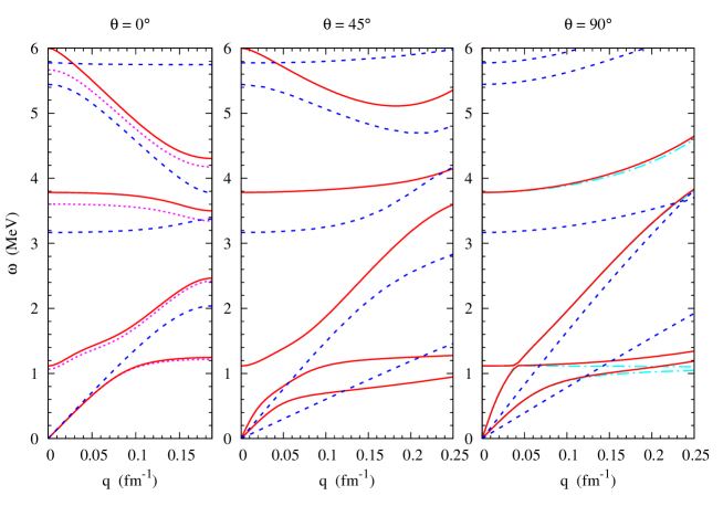
Figure 5: Dispersion relations of the modes propagating along the $z$-axis ($\theta=0$, left), at an angle of $45^{\circ}$, and in the plane parallel to the slabs ($\theta=90^{\circ}$, right). The plain red lines correspond to the present model and the dashed blue lines to the model of Ref. 45, neglecting the Coulomb interaction and assuming an impermeable interface between the different phases. The dotted magenta lines indicate the results of the present model upon neglecting the microscopic entrainment effect and the dash-dotted turquoise line the result neglecting the surface tension.

as functions of $q$ for three different angles $\theta$ between $\bm{\mathrm{q}}$ and the $z$ axis (i.e., $q_{z}=q\cos\theta$ and $q_{\parallel}=\sqrt{q_{x}^{2}+q_{y}^{2}}=q\sin\theta$). The left panel shows the dispersion relation for waves propagating in $z$-direction, i.e. perpendicular to the interfaces between the different slabs. We observe an acoustic branch with an approximately linear dispersion law

$$\omega=u_{1}q$$ (33)

at low energies, and several optical branches with a finite energy for $q=0$, analogously to phonon branches in a crystal. The main differences between the present model (solid red lines) and the previous one[45] (dashed blue lines) are as follows: [(ii)]

Here we use more realistic boundary conditions corresponding to a permeable interface between the two phases, whereas in Ref. 45 neutrons were not allowed to pass from one phase into the other.

We include the Coulomb interaction which was neglected in Ref. 45. Actually, the change of the boundary conditions has only little influence on the energy spectrum, whereas the Coulomb interaction gives rise to an additional mode. Compared with Ref. 45, we have introduced the surface tension, too. The effect of the surface tension is obviously vanishing for modes propagating perpendicular to the interface and maximal for modes propagating along the layers. The effect on the excitation energies is small, see the right panel of Fig. 5, where we display the result for $\sigma=0$ in comparison with the complete calculation. On the other panels the difference is too small to be seen and therefore not shown. The effect of microscopic entrainment is weak, too, as can be seen from the left panel.

Note that within the Wigner-Seitz approximation as discussed in Sec. 2.2, we would only obtain a discrete spectrum corresponding to our spectrum in the case $q=0$. The reason is that in this approximation the coupling between cells is neglected, and thus each cell has the same excitation spectrum. The degeneracy of the modes in each cell is lifted by the coupling between cells, which gives rise to a momentum dependent spectrum as obtained in our approach.

Let us now look at the cases $\theta=45^{\circ}$ and $90^{\circ}$ shown in the central and right panels of Fig. 5. As in Ref. 45, we find now two acoustic modes. The energy of the second acoustic mode can be approximately written as

$$\omega=u_{2}q_{\parallel}=u_{2}q\sin\theta\,,$$ (34)

which means that this mode propagates in a slab with almost no coupling to neighboring slabs.

The two acoustic modes dominate largely the baryonic contributions to the specific heat and exceed in particular the contributions from superfluid neutron quasiparticles. The temperature dependence of the specific heat corresponding to the modes shown in Fig. 5 is displayed in Fig. 6.

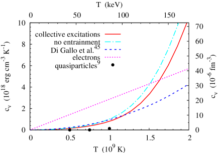
Figure 6: Specific heat as a function of temperature for $n_{B}=0.08$ fm^-3.

We assume here that the temperature dependence of the mode spectrum can be neglected, which should be true for $T\ll\Delta_{n},\Delta_{p}$. The electronic contribution $c_{v,e}=\mu_{e}^{2}T/3$ and the contribution from weakly paired neutron quasiparticles[9] are shown for comparison, too.

At very low temperatures, the specific heat of the collective excitations is approximately given by[45]

$$c_{v,{\mathit{coll}}}\approx aT^{2}+bT^{3}\,,$$ (35)

with $a\approx 3\zeta(3)/\pi u_{2}^{2}L$ and $b\approx 2\pi^{2}/15u_{1}^{3}$. The $T^{3}$ term is the usual acoustic phonon, whereas the “two-dimensional” mode discussed above gives rise to a contribution increasing as $T^{2}$.[45] We note, however, that within our new model the deviations from this approximate formula are stronger than in Ref. 45 for both acoustic modes: the level repulsion due to avoided crossings let them deviate from the purely linear behavior for much smaller momentum values. As a consequence, the approximation (35) is valid only for much smaller temperatures, where the electronic contribution to the specific heat is the most important one. As can be seen from Fig. 6, the additional mode and the resulting flattening of the acoustic modes increase the contribution to the specific heat.

4 Summary and Conclusions

In Sec. 2, we reviewed a couple of existing approaches to describe collective modes in the superfluid inner crust of neutron stars. Considering only a uniform neutron gas within the QRPA, one recovers the Goldstone mode, which is a longitudinal density wave (BA sound) with linear dispersion relation at small $q$, as the lowest lying collective excitation. For a realistic description of the neutron star inner crust, however, its crystalline structure should be considered, i.e. it should be described as a lattice of dense clusters surrounded by a neutron gas. There are several approaches to treat collective excitations of this non-uniform matter involving different kinds of approximations.

In the standard hydrodynamic approach, only coarse-grained quantities are considered, i.e., quantities averaged over many cells. This leads to an effective low-energy theory, in which the superfluid collective modes with linear dispersion relation are coupled to the dynamics of the crystal lattice. However, this effective theory is only valid at very large wavelengths (much larger than the periodicity of the lattice, $L$), and the determination of its coefficients, especially those involving the so-called entrainment, is difficult.

On the other hand, a QRPA calculation within the WS approximation resolves the microscopic structure of each cell. However, it gives the lowest lying collective mode at a finite energy. This is an artefact of treating an isolated cell with a finite radius $R_{{\mathit{WS}}}$. Nevertheless the result is very important since it shows that in a non-uniform system, superfluid hydrodynamics may be used at a microscopic level (i.e., on length scales smaller than $R_{{\mathit{WS}}}$) as long as the coherence length is sufficiently short, i.e., pairing is sufficiently strong.

In Sec. 3, we have presented the approach of superfluid hydrodynamics at a microscopic level in order to develop a model for the collective modes of large and intermediate wavelengths (i.e., larger than or comparable with $L$). In this model, hydrodynamic equations in the clusters and in the neutron gas were matched at the phase boundaries with boundary conditions allowing neutrons to pass from one phase into the other. For simplicity, the model has so far only been solved in the phase of plates. The most striking result is the appearance of an approximately two-dimensional collective mode, which gives a contribution to the specific heat proportional to $T^{2}$ (in contrast to the usual $T^{3}$ behavior) at low temperatures.

There remain many open questions. In particular, in order to better understand the two-dimensional mode, we are developing an effective theory corresponding to our model in the limit of small $q$. This could help to clarify some questions concerning entrainment, too,[43, 44, 36, 37] see the discussion in Sec. 2.3. In addition, we plan to apply our hydrodynamic model to other geometries such as the crystalline phase or the phase of rods.

The latter point is essential in order to make contact with astrophysical observations, since it would allow one to determine heat transport properties in the entire inner crust, necessary for modeling neutron star thermal evolution. Properties of the crust influence the cooling process mainly during the first 50-100 years, when the crust stays hotter that the core which cools down very efficiently via neutrino emission (see, e.g., Ref. 5). Heat transport in the crust is the key ingredient to explain the afterburst relaxation in X-ray transients, too.[6, 7] As microscopic ingredients for the models of the thermal relaxation of the crust, in addition to the specific heat, thermal conductivity would be needed, and to less extent neutrino emissivities. Although the contribution of collective modes to heat transport properties exceeds largely that of superfluid quasiparticles, it is to be expected that in almost the whole crust electronic contributions remain dominant, except in presence of a neutron star magnetic field of the order $10^{13}$ G or higher,[56] which is the case for many observed neutron stars. Therefore it would be interesting to extend the present model to a magnetised environment, too.

Appendix A Microscopic Input for the Model of Section 3

As microscopic input, we need the equation of state, i.e., the relation between the densities $n_{a}$ and the chemical potentials $\mu_{a}$. As in Ref. 45, in our concrete numerical examples, we use the results of the work by Avancini et al.[42] for the equilibrium configurations. They evaluate the structure of the pasta phases for charge neutral matter in $\beta$ equilibrium using a density dependent relativistic mean-field model, the DDH$\delta$ model (originally called DDH$\rho\delta$), for the nuclear interaction.[57, 58, 42] In order to be consistent, we shall calculate the chemical potentials $\mu_{a}$ with the same interaction. The entrainment coefficients within this model, evaluated following the approach in Refs. 52, 51, are given by

$$M_{ab}=m^{L}_{a}\delta_{ab}+n_{b}\Big{(}\frac{\Sigma_{R}}{n_{B}}+\frac{\Gamma^{2}_{\omega}}{m^{2}_{\omega}}+\frac{t_{a}t_{b}}{4}\,\frac{\Gamma^{2}_{\rho}}{m^{2}_{\rho}}\Big{)}\,,$$ (36)

where $n_{B}=n_{n}+n_{p}$ denotes the baryon density, $t_{n}=-1$ and $t_{p}=1$. The Landau effective masses are denoted $m^{L}_{a}=\sqrt{p^{2}_{Fa}+m_{a}^{D\,2}}$, not to be confused with the Dirac effective masses $m^{D}_{a}$. The Fermi momenta are represented by $p_{Fa}$ and $\Gamma_{i}=g_{i}h_{i}(n_{B})$ are the meson-nucleon coupling constants of the DDH$\delta$ model, see Ref. 42. The term $\Sigma_{R}$, not present in the expressions given in Refs. 52, 51, arises from the density dependence of the coupling constants and appears in the Landau effective masses, too,

$$m^{L}_{a}=\mu_{a}-\frac{\Gamma^{2}_{\omega}}{m^{2}_{\omega}}n_{B}-t_{a}\frac{\Gamma^{2}_{\rho}}{4m_{\rho}^{2}}(n_{p}-n_{n})-\Sigma_{R}\,.$$ (37)

and an explicit expression can be found in Ref. 42.

References

- [1] N. Chamel and P. Haensel, Living Rev. Relativity 11, 10 (2008).
- [2] J. W. Negele and D. Vautherin, Nucl. Phys. A 207, 298 (1973).
- [3] D. G. Ravenhall, C. J. Pethick, and J. R. Wilson, Phys. Rev. Lett. 50, 2066 (1983).
- [4] K. Oyamatsu, Nucl. Phys. A 561, 431 (1993).
- [5] D. G. Yakovlev, O. Y. Gnedin, A. D. Kaminker, and A. Y. Potekhin, AIP Conf. Proc. 983, 379 (2008).
- [6] P. S. Shternin, D. G. Yakovlev, P. Haensel, and A. Y. Potekhin, Mon. Not. R. Astron. Soc. 382, L43 (2007).
- [7] E. F. Brown and A. Cumming, Astrophys. J. 698, 1020 (2009).
- [8] A. L. Fetter and J. D. Walecka, Quantum Theory of Many-particle Systems, (McGraw-Hill, New York, 1971).
- [9] M. Fortin, F. Grill, J. Margueron, D. Page, and N. Sandulescu, Phys. Rev. C 82, 065804 (2010).
- [10] D. Page, M. Prakash, J. M. Lattimer and A. W. Steiner, Phys. Rev. Lett. 106 (2011) 081101.
- [11] P. S. Shternin, D. G. Yakovlev, C. O. Heinke, W. C. G. Ho and D. J. Patnaude, Mon. Not. Roy. Astron. Soc. 412 (2011) L108.
- [12] C. García-Recio, J. Navarro, Nguyen Van Giai, and L. L. Salcedo, Ann. Phys. (N.Y.) 214, 293 (1992).
- [13] A. Pastore, M. Martini, V. Buridon, D. Davesne, K. Bennaceur, and J. Meyer, Phys. Rev. C 86, 044308 (2012).
- [14] J. Margueron, I. Vidaña, and I. Bombaci, Phys. Rev. C 68, 055806 (2003).
- [15] P. Ring and P. Schuck, The Nuclear Many-Body Problem (Springer, Berlin, 1980).
- [16] J. Keller and A. Sedrakian, Phys. Rev. C 87, 045804 (2013).
- [17] M. Baldo and C. Ducoin, Phys. Rev. C 84, 035806 (2011).
- [18] N. Martin and M. Urban, Phys. Rev. C 90, 065805 (2014).
- [19] P. W. Anderson, Phys. Rev. 112, 1900 (1958).
- [20] N. N. Bogoliubov, V. V. Tolmachev, and D. V. Shirkov, A New Method in the Theory of Superconductivity (Consultants Bureau, New York, 1959).
- [21] R. Combescot, M. Yu. Kagan, and S. Stringari, Phys. Rev. A 74, 042717 (2006).
- [22] M. M. Forbes and R. Sharma, Phys. Rev. A 90, 043638 (2014).
- [23] P. Nozières, Theory of interacting Fermi systems, (Benjamin, New York, 1963)
- [24] L. P. Gor’kov and T. K. Melik-Barkhudarov, Sov. Phys. JETP 13, 1018 (1961).
- [25] A. Gezerlis and J. Carlson, Phys. Rev. C 81, 025803 (2010).
- [26] J. Goldstone, A. Salam, and S. Weinberg, Phys. Rev. 127, 965, (1962).
- [27] S. Weinberg, The Quantum Theory of Fields, Volume II: Modern Applications (Cambridge University Press, Cambridge, 1996).
- [28] E. M. Lifshitz and L. P. Pitaevskii, Statistical Physics, Part 2, Landau Lifshitz Course of Theoretical Physics, Vol. 9 (Pergamon Press, Oxford, 1980).
- [29] P. Debye, Ann. Phys. (Leipzig) 344, 789 (1912).
- [30] N. W. Ashcroft and N. D. Mermin, Solid state physics (Saunders College, Fort Worth, 1976).
- [31] N. Sandulescu, Nguyen Van Giai, and R. J. Liotta Phys. Rev. C 69, 045802 (2004).
- [32] E. Khan, N. Sandulescu, and Nguyen Van Giai, Phys. Rev. C 71, 042801(R) (2005).
- [33] M. Grasso, E. Khan, and M. Urban, Phys. Rev. A 72, 043617 (2005).
- [34] C. Menotti, P. Pedri, and S. Stringari, Phys. Rev. Lett. 89, 250402 (2002).
- [35] B. Carter, N. Chamel, P. Haensel, Nucl. Phys. A 748 675 (2005).
- [36] N. Chamel, Nucl. Phys. A 747 109 (2005).
- [37] N. Chamel, Phys. Rev. C 85, 035801 (2012).
- [38] V. Cirigliano, S. Reddy, and R. Sharma, Phys. Rev. C 84, 045809 (2011).
- [39] N. Chamel, D. Page, and S. Reddy, Phys. Rev. C 87, 035803 (2013).
- [40] D. Kobyakov and C.J. Pethick, Phys. Rev. C 87, 055803 (2013).
- [41] D. Page and S. Reddy, in Neutron Star Crust, ed. C. Bertulani and J. Piekarewicz (Nova Science Publishers, Hauppauge, 2012), ch. 14 [e-print arxiv:1201.5602].
- [42] S. S. Avancini, L. Brito, J. R. Marinelli, D. P. Menezes, M. M. W. de Moraes, C. Providência, and A. M. Santos, Phys. Rev. C 79, 035804 (2009).
- [43] P. Magierski, Int. J. Mod. Phys. E 13, 371 (2004) [e-print arXiv:astro-ph/0312643].
- [44] P. Magierski and A. Bulgac, Acta Phys. Polon. B 35, 1203 (2004) [e-print arXiv:astro-ph/0312644].
- [45] L. Di Gallo, M. Oertel, and M. Urban, Phys. Rev. C 84, 045801 (2011).
- [46] L. D. Landau and E. M. Lifshitz, Fluid Mechanics, Landau Lifshitz Course of Theoretical Physics, Vol. 6 (Pergamon Press, Oxford, 1987).
- [47] J. D. Jackson, Classical Electrodynamics (Wiley, New York, 1975).
- [48] A. Lazarides and B. Van Schaebroeck, Phys. Rev. A 77, 041602(R) (2008).
- [49] R. Prix, Phys. Rev. D 69, 043001 (2004).
- [50] R. Prix, Phys. Rev. D 71, 083006 (2005).
- [51] M. Gusakov, E. Kantor, P. Haensel, Phys. Rev. C 79, 055806 (2009).
- [52] G. L. Comer, R. Joynt, Phys. Rev. D 68, 023002 (2003).
- [53] A. F. Andreev and E. P. Bashkin, Sov. Phys. JETP 42, 164 (1975).
- [54] N. Chamel and P. Haensel, Phys. Rev. C 73, 045802 (2006).
- [55] M. Borumand, R. Joynt, and W. Kluźniak, Phys. Rev. C 54, 2745 (1996).
- [56] D. N. Aguilera, V. Cirigliano, J. A. Pons, S. Reddy and R. Sharma, Phys. Rev. Lett. 102 091101 (2009).
- [57] T. Gaitanos, M. Di Toro, S. Typel, V. Baran, C. Fuchs, V. Greco, and H. H. Wolter, Nucl. Phys. A 732, 24 (2004).
- [58] S. S. Avancini, L. Brito, D. P. Menezes, C. Providência, Phys. Rev. C 70, 015203 (2004).