An Efficient Algorithm for Video Super-Resolution Based On a Sequential Model

Abstract

In this work, we propose a novel procedure for video super-resolution, that is the recovery of a sequence of high-resolution images from its low-resolution counterpart. Our approach is based on a “sequential” model (i.e., each high-resolution frame is supposed to be a displaced version of the preceding one) and considers the use of sparsity-enforcing priors. Both the recovery of the high-resolution images and the motion fields relating them is tackled. This leads to a large-dimensional, non-convex and non-smooth problem. We propose an algorithmic framework to address the latter. Our approach relies on fast gradient evaluation methods and modern optimization techniques for non-differentiable/non-convex problems. Unlike some other previous works, we show that there exists a provably-convergent method with a complexity linear in the problem dimensions. We assess the proposed optimization method on several video benchmarks and emphasize its good performance with respect to the state of the art.

1 Introduction

Super resolution (SR) aims at reconstructing high-resolution (HR) images from distorted low-resolution (LR) observations. This type of methodology dates back to the 70’s with the pioneering work of Gerchberg [27] and Santis&Gori [17]. Since then, super resolution has been applied to a large variety of applicative domains, including infrared [29], medical [46], satellite and aerial [42, 51] imaging. We refer the reader to [38] for a pretty comprehensive overview of the works dealing with SR.

One can distinguish between different setups in the domain of super resolution. “Single-frame” super resolution aims at computing an enhanced version of some HR image from the observation of one single LR image, see e.g., [18, 30, 43]. On the other hand, the “multi-frame” paradigm typically focusses on the recovery of one HR image by exploiting the observations of several LR frames, see e.g., [22, 41, 24, 26, 37, 53, 33]. Finally, the “video” super resolution problem consists in estimating a sequence of HR images from the observations of their LR counterparts. We consider the latter paradigm in this paper.

From a conceptual point of view, a simple (but valid) solution to address video super-resolution consists in applying single-frame or multi-frame procedures on each frame of the HR sequence to recover. This strategy was for example considered in [22, 41, 24, 26, 37, 53, 33]. Nevertheless, this approach may fail in properly exploiting the strong temporal correlations existing between the (successive) frames of the HR sequence. Hence, procedures specifically dedicated to accounting for these dependencies have been proposed in the literature, see [50, 20, 21, 55, 62, 23, 28, 49, 48]. A central element is the “sequential” model linking the frames of the HR sequence. More specifically, in most of these methods, the frames of the HR sequence are supposed to obey a dynamical model where each HR image is seen as a displaced version (by some unknown motion field) of the preceding one (see section 3 for a detailed description). This is in contrast with the standard multi-frame model where each LR observation is assumed to be a LR displaced version of one given reference frame.

The practical exploitation of the “sequential” model nevertheless faces a certain number of bottlenecks. The most stringent one is probably the model dimensionality: because it accounts for the temporal evolution of each HR frame, the number of variables involved in the sequential model may become very large. This makes video SR based on sequential models pretty challenging. As a matter of fact, in comparison with the huge number of papers dealing with SR, only a few have focussed on this particular problem, see [50, 20, 21, 55, 62, 23, 28, 49, 48]. In [50], the authors modeled the dependence between the different images of the sequence as a Gaussian process and provided an efficient implementation in the Fourier domain. Other contributions relied on adaptive-filtering techniques, see [20, 21, 55, 62, 23, 28]. In this line of thought, most of the contributions cited above considered that the HR sequence is ruled by a state-space sequential model and the authors derived estimation procedures inspired by the well-known Kalman filter. The standard Kalman updates leading to a prohibitive complexity in the context of video SR, Elad and co-authors published a series of papers [20, 21, 23] in which they proposed updates having a linear complexity in the problem dimensions. Their approach is based on some approximations of the model and/or Kalman updates (e.g., uniform translational motion [23], noise-free evolution model [21], etc). In [49, 48], the authors considered a local approximation of the state-space sequential model by using steering kernel regression on the LR observations.

In this paper, we provide an approximation-free methodological framework exploiting a sequential model for video SR. We express the unknown HR sequence as the solution of a constrained optimization problem and propose an iterative procedure to solve the latter. Our method is provably convergent (to a local minimum of the problem) and has a tractable complexity per iteration (i.e., linear in the problem dimensions). The proposed framework encompasses two important ingredients of video SR, namely: i) a precise characterization of the motion fields linking the successive frames of the sequence; ii) the exploitation of proper priors on the unknowns of the problem. These two ingredients lead to additional difficulties (in top of the large dimensionality) since they typically introduce non-convex and non-smooth terms in the cost function to minimize. We elaborate on these points in the two next paragraphs.

A precise characterization of the model connecting the different images of the HR sequence is crucial for the success of video SR. Typically, videos are characterized by non-global motions. This is in contrast with many standard SR models of the literature which assume global motions (e.g., translation [1], affine [58] or projection [13]), well-suited to still image reconstruction. The imaging model in video SR thus takes a more-involved form and has to be considered with care. In particular, the estimation of the motion between two consecutive frames is usually tantamount to solving an optical-flow problem [4]. Embedding motion estimation in the SR reconstruction introduces new difficulties: i) it increases the problem dimensionality since two additional unknowns (the displacement in each direction) have to be estimated for each pixel of the HR images; ii) it typically introduces non-linearities in the image formation model. These obstacles are particularly prominent in the case of a sequential model because of the nested structure of the unknowns dependencies. As a consequence, until recently, motion estimation has been overlooked and considered as a side problem in many SR contributions involving either muti-frame or sequential models (see e.g., [41, 22, 20, 21, 55, 62, 24, 23, 28, 53, 37]) with the exception of e.g., [4, 26, 31, 34] .

Interestingly, several authors have emphasized the importance of accurate motion estimation in the video SR process and provided studies of the sensibility of adaptive filtering techniques to the latter, see [62, 14, 15, 16]. In this paper, we show that the motion estimation can be included in our video SR problem without significantly increasing the computational cost.

Another important ingredient for the success of video SR is the definition of proper priors on (some of) the unknowns of the problem. Indeed, video SR is a naturally ill-posed problem: typical setups impose the observation of (at most) one LR image per frame of the HR sequence; hence, if the motion between the different frames is unknown, it is easy to see that the number of variables which have to be estimated is well beyond the number of observations. In order to tackle this difficulty, a well-known technique consists in resorting to prior information on the sought quantities. This type of approach has been used extensively (but not only) in the context of single-image SR, where an HR image has to be reconstructed from one single LR observation. First methodologies based on prior information date back to the 70’s [27, 17]. Since then, many types of priors have been studied, including Markov random fields [47], total variation [37, 60, 34], morphological [44] or sparse [59, 43] models, etc. Among the most effective models in the literature, many rely on the minimization of some non-differentiable functions. It is for example the case of SR techniques based on sparse representations where the decomposition coefficients of the sought quantity in a redundant dictionary are commonly penalized by an $\ell_{1}$ norm, see e.g., [25]. Another example is total variation where the $\ell_{1}$ norm is applied to the gradient of the sought images/motions, see e.g., [34]. The introduction of non-differentiable functions in the SR reconstruction leads to new conundrums since standard optimization techniques for smooth problems can no longer be applied. As mentioned previously, we address this problem in the paper as well. Hereafter, we mainly focus on problems involving an $\ell_{1}$ norm, although other non-differentiable convex functions could be processed using a procedure similar to the one exposed in this paper.

In summary, in this paper we propose a methodological framework for video SR based on a sequential model. We consider the estimation of both a sequence of HR images and the motion fields relating them, while allowing for some non-differential terms in the cost function. Our approach is based on the combination of several modern optimization tools: fast gradient computation [6], the “Alternating Direction Method of Multipliers” [7] for large-scale non-differentiable convex problems, and a recent procedure for non-convex and non-differentiable optimization proposed by Attouch et al. in [2, 3]. The resulting algorithm is ensured to converge to a local minimum of the problem while having a linear complexity per iteration in the problem dimensions. We illustrate the good behavior of the proposed method with respect to other techniques of the state of the art in several setups.

The rest of the paper is organized as follows. We introduce the notations used throughout the paper in section 2. In section 3, we present the sequential model considered in our subsequent derivations. In section 4, we express the video SR problem as a constrained optimization problem and provide a numerical procedure to solve it. The overall procedure is described in subsection 4.3 whereas two important algorithmic building blocks are presented in subsections 4.1 and 4.2. The numerical evaluation of the proposed method is carried out in section 5 for different experimental setups.

2 Notations

The notational conventions adopted in this paper are as follows. Italic lowercase indicates a scalar quantity, as in $a$; boldface lowercase (resp. uppercase) indicates a vector (resp. matrix) quantity, as in $\mathbf{a}$ (resp. $\mathbf{A}$). The $n$-dimensional vector of zeroes and identity matrix will be written as $\mathbf{0}_{n}$ and $\mathbf{I}_{n}$. The $i$-th element of vector $\mathbf{a}$ is denoted $\mathbf{a}(i)$; similarly $\mathbf{A}(i,j)$ is the element of $\mathbf{A}$ located at row $i$ and column $j$. The exponent ^∗ denotes the transpose operation. A subscript notation, as in $\mathbf{a}_{t}$, will refer to the member of some sequence $\{\mathbf{a}_{t}\}_{t=0}^{T}=\{\mathbf{a}_{0},\mathbf{a}_{1},\cdots,\mathbf{a}_{T}\}$.

Calligraphic letters, as $\mathcal{H}$, denote functions. The subscript notation $\mathcal{H}_{i}$ may either denote the $i$-th element of a set $\{\mathcal{H}_{i}\}_{i}$ or the $i$-th component of a multidimensional function $\mathcal{H}:\mathds{R}^{m}\to\mathds{R}^{n}$; the distinction between these two notations is usually clear from the context. The Jacobian matrix of $\mathcal{H}:\mathds{R}^{m}\to\mathds{R}^{n}$ evaluated at $\tilde{\mathbf{a}}$, denoted by $\nabla_{\mathbf{a}}\mathcal{H}(\tilde{\mathbf{a}})$, is defined as:

$$\nabla_{\mathbf{a}}\mathcal{H}(\tilde{\mathbf{a}})=\begin{pmatrix}\partial_{{\mathbf{a}}(1)}\mathcal{H}_{1}(\tilde{\mathbf{a}})&\cdots&\partial_{{\mathbf{a}}(m)}\mathcal{H}_{1}(\tilde{\mathbf{a}})\\ \vdots&&\vdots\\ \partial_{{\mathbf{a}}(1)}\mathcal{H}_{n}(\tilde{\mathbf{a}})&\cdots&\partial_{{\mathbf{a}}(m)}\mathcal{H}_{n}(\tilde{\mathbf{a}})\end{pmatrix}\in\mathds{R}^{n\times m},$$

where $\partial_{v}$ is the partial derivative operator with respect to $v$. We use the notation $\nabla_{\mathbf{a}}\mathcal{H}^{*}(\tilde{\mathbf{a}})$ to denote the transpose of $\nabla_{\mathbf{a}}\mathcal{H}(\tilde{\mathbf{a}})$.

3 Model

Let $\mathbf{x}_{t}\in\mathds{R}^{n}$ be the image at time $t$ of an HR video sequence rearranged into a $n$-dimensional vector, with $t\in\{0,\ldots,T\}$. Let us suppose that we capture noisy and low-resolution (LR) observations $\mathbf{y}_{t}\in\mathds{R}^{m}$ with $m\leq n$ of the HR sequence: $\forall t\in\{0,\ldots,T\}$,

$$\mathbf{y}_{t}=\mathcal{H}(\mathbf{x}_{t})+\boldsymbol{\eta}_{t},$$ (1)

where $\boldsymbol{\eta}_{t}\in\mathds{R}^{m}$ stands for some noise and $\mathcal{H}:\mathds{R}^{n}\rightarrow\mathds{R}^{m}$ denotes a linear function, which is the composition of a low-pass filtering and a sub-sampling operation. We focus on the problem of recovering the HR sequence $\{\mathbf{x}_{t}\}_{t=0}^{T}$ from the LR observations $\{\mathbf{y}_{t}\}_{t=0}^{T}$.

Without any additional information, this problem is ill-conditioned since the number of unknowns (that is $(T+1)n$) is larger than the number of observations (that is $(T+1)m$). One way to circumvent this problem is to take into account the relation existing between the HR images at different time instants. More specifically, as part of a video, we can assume that two consecutive images obey the following sequential model:

$$\mathbf{x}_{t}=\mathcal{P}(\mathbf{x}_{t+1},\mathbf{d}_{t+1})+\boldsymbol{\epsilon}_{t+1},$$ (2)

where $\mathcal{P}:\mathds{R}^{n}\times\mathds{R}^{2n}\rightarrow\mathds{R}^{n}$ is a “warping” function characterized by a displacement $\mathbf{d}_{t+1}\in\mathds{R}^{2n}$, and $\boldsymbol{\epsilon}_{t+1}\in\mathds{R}^{n}$ is some noise. The choice of $\mathcal{P}$ is usually motivated by some conservation property, as for example the preservation of the pixel intensity along the displacement. One particular instance of function $\mathcal{P}$, that we will consider in the sequel, is based on the well-known “Displaced Frame Difference” model. More specifically, this model assumes that the $s$-th component of $\mathcal{P}(\mathbf{x}_{t},\mathbf{d}_{t})$ admits the following series representation:

$$\mathcal{P}_{s}(\mathbf{x}_{t},\mathbf{d}_{t})=\sum_{i\in\mathcal{V}(\chi(s)+\mathbf{d}_{t}(s))}\mathbf{x}_{t}(i)\psi_{i}(\chi(s)+\mathbf{d}_{t}(s)),$$ (3)

where $\chi:\mathds{R}\times\mathds{R}\to\mathds{R}$ is a function returning the spatial position corresponding to index $s$, $\mathcal{V}(\chi(s)+\mathbf{d}_{t}(s))$ denotes a subset of indices corresponding to the “neighborhood” of point $\chi(s)+\mathbf{d}_{t}(s)$ and $\{\psi_{i}\}_{i=1}^{n}$ with $\psi_{i}:\mathds{R}\times\mathds{R}\to\mathds{R}$ is a family of bi-dimensional polynomial interpolation functions. In this case, (2)-(3) models the fact that $\mathbf{x}_{t}$ can be seen as a displaced version of $\mathbf{x}_{t+1}$ plus some additive noise. Let us note that $\mathcal{P}$, as defined in (3), is linear in $\mathbf{x}_{t}$ and polynomial in $\mathbf{d}_{t}$; it is thus a bi-polynomial function. Let us also mention that $\mathcal{V}$ typically only contains a few elements that is $|\mathcal{V}|\ll n$, where $|\mathcal{V}|$ denotes the cardinality of $\mathcal{V}$; this observation will play an important role in the sequel for the analysis of the complexity of the proposed SR methodology.

The noise $\boldsymbol{\epsilon}_{t+1}$ in (2) accounts for all the modifications of the image $\mathbf{x}_{t}$ which cannot be inferred from $\mathbf{x}_{t+1}$ and $\mathbf{d}_{t+1}$. This includes pixel occlusions, interpolation errors or variations of the scene illumination. Notice that, in practice, the choice of $\mathcal{P}$ should be made such that the residual noise $\boldsymbol{\epsilon}_{t+1}$ is as small as possible. In particular, if $\boldsymbol{\epsilon}_{t+1}=0$ (and $\mathbf{d}_{t+1}$ is known), $\mathbf{x}_{t}$ is entirely determined from $\mathbf{x}_{t+1}$ $\forall t$. Recovering the whole sequence $\{\mathbf{x}_{t}\}_{t=0}^{T}$ is then tantamount to recovering the last image $\mathbf{x}_{T}$. In such a case, the number of unknowns is therefore reduced to $n$ and the recovery of the HR sequence from the LR images may be possible.

Another option to decrease the ill-possedness of the video SR problem consists in restricting the family of signals to which the “initial condition” $\mathbf{x}_{T}$ belongs. We will in particular consider the case where $\mathbf{x}_{T}$ is assumed to be sparse in some (possibly redundant) dictionary $\mathbf{D}\in\mathds{R}^{n\times q}$, that is

$$\mathbf{x}_{T}=\mathbf{D}\mathbf{c}\quad\mbox{for some $\mathbf{c}\in\mathds{R}^{q}$ such that $\|\mathbf{c}\|_{0}\ll n$},$$ (4)

where $\|.\|_{0}$ is the so-called “$\ell_{0}$ norm”, which returns the number of nonzero coefficients of its argument. Dealing with $\|.\|_{0}$ leads to combinatorial optimization problems. Hereafter we will thus consider the $\ell_{1}$ norm, which is a well-known surrogate to the $\ell_{0}$ norm. In particular, if the sparsity of the sought vector is large enough, there exists an equivalence between the solution of the problems involving the $\ell_{0}$ and $\ell_{1}$ norms, see [25].

Finally, let us mention that the displacement $\mathbf{d}_{t}$ between two successive images is rarely known in practice. It must therefore be inferred from the received LR images $\{\mathbf{y}_{t}\}_{t=0}^{T}$. This may seem to be counterproductive since the estimation of $\mathbf{d}_{t}$ implies an increase of the number of unknowns of $2n$ elements per time step. One way to circumvent this problem consists again in constraining $\mathbf{d}_{t}$ to belong to a restricted family of signals. In this paper, we consider an implicit restriction by enforcing some non-negative function of $\mathbf{d}_{t}$ to be small. More specifically, we assume that the sought displacement is such that $\mathcal{R}(\mathbf{G}^{*}\mathbf{d}_{t})$ is “small”, where $\mathbf{G}=[\mathbf{g}_{1},\ldots,\mathbf{g}_{h}]\in\mathds{R}^{2n\times h}$ is some linear “analysis” operator and $\mathcal{R}:\mathds{R}^{h}\rightarrow\mathds{R}$ is a non-negative function. We note that this approach is commonly adopted in the computer-vision literature in which many options for $\mathcal{R}$ and $\mathbf{G}$ have been proposed, see [5]. This approach was also used in the “multi-frame” setting [37, 34] where the motions between the reference HR frame and the LR observations were penalized to have a small TV-norm. In the sequel, we will focus on the following choice for $\mathbf{G}$ and $\mathcal{R}$: the elements of $\mathbf{G}^{*}\mathbf{d}_{t}$ will correspond to the spatial gradients of (an interpolation of) $\mathbf{d}_{t}$ at each point of the pixel grid; $\mathcal{R}(\mathbf{G}^{*}\mathbf{d}_{t})$ takes the following form:

$$\mathcal{R}(\mathbf{G}^{*}\mathbf{d}_{t})\triangleq\sum_{i=1}^{n}\mathbf{w}(i)\Bigl{|}\sum_{j\in\mathcal{S}_{i}}(\mathbf{g}^{*}_{j}\mathbf{d}_{t})^{2}\Bigr{|}^{\frac{p}{2}},\quad p\geq 0,$$ (5)

where $\mathbf{w}$ is defined as a vector of weights and $\mathcal{S}_{i}$’s denote disjoint subsets of elements of $\{1,\ldots,h\}$. Index $i$ represents a location on the pixel grid. The subset $\mathcal{S}_{i}$ typically gathers 4 elements corresponding to the 2 spatial gradients of the 2 components of motion $\mathbf{d}_{t}$ at the location indexed by $i$. For $p=2$, these choices are equivalent to constraining the spatial gradient of the displacement field $\mathbf{d}_{t}$ by a quadratic penalization [56], whereas the case $p=1$ corresponds to the weighted total variation (TV) approach suggested in [61].

In summary, (1)-(4) together with the definition of $\mathbf{G}$ and $\mathcal{R}$ specify our prior/observation model. In the next section, we will present a low-complexity methodology exploiting this model to recover the HR sequence from the collected observations $\{\mathbf{y}_{t}\}_{t=0}^{T}$. More specifically, we will assume that the unknowns of the problem include the HR sequence $\{\mathbf{x}_{t}\}_{t=0}^{T}$, the sequential noise $\{\boldsymbol{\epsilon}_{t}\}_{t=1}^{T}$, the displacements $\{\mathbf{d}_{t}\}_{t=1}^{T}$ and the decomposition vector $\mathbf{c}$. All the other parameters of the problem will be supposed to be known, although they could easily be included as additional unknowns without introducing any conceptual problem in the proposed methodology.

4 The Estimation Procedure

In this section, we expose our methodology to estimate the HR sequence by exploiting the model described in section 3. Our approach is based on the resolution of a constrained optimization problem. We introduce the following shorthand notations: $\mathbf{x}\triangleq\{\mathbf{x}_{t}\}_{t=0}^{T}$, $\boldsymbol{\epsilon}\triangleq\{\boldsymbol{\epsilon}_{t}\}_{t=1}^{T}$ and $\mathbf{d}\triangleq\{\mathbf{d}_{t}\}_{t=1}^{T}$. Our SR reconstruction procedure relies on the following constrained optimization problem:

$$\operatorname*{arg\,min}_{(\mathbf{x},\boldsymbol{\epsilon},\mathbf{d},\mathbf{c})}\mathcal{J}(\mathbf{x},\boldsymbol{\epsilon},\mathbf{d},\mathbf{c})\quad\textrm{s.t.}\ \left\{\begin{aligned} &\mathbf{x}_{t}=\mathcal{P}(\mathbf{x}_{t+1},\mathbf{d}_{t+1})+\boldsymbol{\epsilon}_{t+1},&\hskip 5.69046pt0\leq t\leq T-1,\\ &\mathbf{x}_{T}=\mathbf{D}\mathbf{c},&\hskip 5.69046pt\end{aligned}\right.$$ (6)

where

$$\mathcal{J}(\mathbf{x},\boldsymbol{\epsilon},\mathbf{d},\mathbf{c})\triangleq \sum_{t=0}^{T}\|\mathcal{H}(\mathbf{x}_{t})-\mathbf{y}_{t}\|^{2}_{2}+\alpha_{1}\sum_{t=1}^{T}\|\boldsymbol{\epsilon}_{t}\|_{p}^{p}+\alpha_{2}\sum_{t=1}^{T}\mathcal{R}(\mathbf{G}^{*}\mathbf{d}_{t})+\alpha_{3}\|\mathbf{c}\|^{p}_{p},$$

for some $\alpha_{j}\geq 0$, $j\in\{1,2,3\}$, and $p\geq 0$. Let us make a few comments about (6). The first constraint ensures that the images of the HR sequence verify the sequential model (2); the second enforces that prior model (4) is satisfied. Each term in the cost function $\mathcal{J}(\mathbf{x},\boldsymbol{\epsilon},\mathbf{d},\mathbf{c})$ has a clear physical meaning: the first term penalizes the discrepancies between the predicted and the received observations; the second penalizes the noise on the sequential model; the third enforces the displacement to have some regularity and the last one constrains $\mathbf{c}$ to have some desirable properties (depending on the choice of $p$). For example, setting $p\in[0,1]$ typically promotes the sparsity of $\mathbf{c}$, see [25]. Because sparsity has revealed to be a good prior in a number of works, in the following our main objective is to find a solution to (6) with $p=1$.

Problem (6) involves a huge number of unknowns (namely $(4T+1)n+q$ variables if $\mathbf{x},\boldsymbol{\epsilon},\mathbf{d},\mathbf{c}$ have to be estimated). Hence, solving (6) may be critical even for reasonable problem sizes: for instance, considering images of $n=2^{8}\times 2^{8}$ pixels, a non-redundant dictionary, i.e., $q=n$ and a sequence length $T=2^{4}$, we have that the number of variables involved in the optimization problem grows up to roughly $2^{22}$. Clearly, such a high-dimensional problem can only be addressed by specifically-dedicated procedures. In subsection 4.3, we propose an overall methodology to solve (6) efficiently with $p=1$. Our approach is based on the combination of several modern optimization tools, described in subsections 4.1 and 4.2. More specifically, the building blocks presented in subsections 4.1 and 4.2 tackle simplified versions of problem (6), which appear as intermediate steps in the overall procedure described in section 4.3. We briefly comment on these intermediate problems in the next paragraphs.

In section 4.1, we consider the case where $p=2$ in (6), that is all the functions are differentiable. In such a case, we show that the gradient of the cost function associated to an (equivalent) unconstrained version of (6) can be evaluated efficiently by resorting to optimal control techniques [6]. More specifically, we emphasize that the complexity associated to the evaluation of the gradient of the cost function remains linear in the problem dimensions, for many setups of practical interest.

In section 4.2, we focus on the case where $\mathbf{d}$ is known but $p=1$. The corresponding optimization problem is then convex but not differentiable. Building on our derivations in section 4.1, we emphasize that this type of problem can be nicely addressed by resorting to the so-called “Alternating Direction of Multipliers Method” (ADMM) [7], a modern optimization technique proposed to handle large-scale non-differentiable optimization problems.

Finally, in section 4.3, we consider the general problem (6), where $\mathbf{x},\boldsymbol{\epsilon},\mathbf{d},\mathbf{c}$ have to be estimated and $p=1$. In this case, (6) is non-convex (because the term $\mathcal{P}(\mathbf{x}_{t+1},{\mathbf{d}_{t+1}})$ appearing in the constraints is bi-polynomial) and non-differentiable. In order to address this problem, we resort to an optimization procedure introduced by Attouch et al. [2, 3], and particularized in [45] to multi-frame SR. The procedure is iterative and exploits the building blocks derived in sections 4.1 and 4.2 to solve intermediate problems. The complexity per iteration is linear in the problem dimensions. Moreover, from the arguments exposed in [45], it can be shown that the proposed procedure is convergent to a critical point of the problem.

4.1 The First Building Block

In this section, we assume that $p=2$ (so that all the functions appearing in (6) are differentiable) and show that an efficient resolution of (6) via gradient descent algorithms exists. Our approach is based on fast gradient evaluation techniques as exposed in [6].

In order to present our methodology, we first reformulate (6) as an (equivalent) unconstrained problem. Notice that, because of the constraints in problem (6), any $\mathbf{x}_{t}$ can be expressed as a deterministic function of $\mathbf{c}$ and $\{\boldsymbol{\epsilon}_{t^{\prime}},\mathbf{d}_{t^{\prime}}\}_{t^{\prime}=t+1}^{T}$. In other words, there exists a function $\mathcal{Q}(\boldsymbol{\epsilon},\mathbf{d},\mathbf{c}):\mathds{R}^{Tn}\times\mathds{R}^{2Tn}\times\mathds{R}^{q}\rightarrow\mathds{R}^{(T+1)n}$ such that, given $\boldsymbol{\epsilon},\mathbf{d}$ and $\mathbf{c}$, $\mathbf{x}=\mathcal{Q}(\boldsymbol{\epsilon},\mathbf{d},\mathbf{c})$ is the unique vector satisfying the constraints in (6). As a consequence, (6) can also be equivalently expressed as

$$\operatorname*{arg\,min}_{(\boldsymbol{\epsilon},\mathbf{d},\mathbf{c})}\mathcal{J}(\boldsymbol{\epsilon},\mathbf{d},\mathbf{c}),$$ (7)

where

$$\mathcal{J}(\boldsymbol{\epsilon},\mathbf{d},\mathbf{c}) \triangleq\mathcal{J}(\mathbf{x}=\mathcal{Q}(\boldsymbol{\epsilon},\mathbf{d},\mathbf{c}),\boldsymbol{\epsilon},\mathbf{d},\mathbf{c}),$$

$$=\sum_{t=0}^{T}\|\mathcal{H}(\mathcal{Q}_{t}(\boldsymbol{\epsilon},\mathbf{d},\mathbf{c}))-\mathbf{y}_{t}\|^{2}_{2}+\alpha_{1}\sum_{t=1}^{T}\|\boldsymbol{\epsilon}_{t}\|_{p}^{p}$$

$$+\alpha_{2}\sum_{t=1}^{T}\mathcal{R}(\mathbf{G}^{*}\mathbf{d}_{t})+\alpha_{3}\|\mathbf{c}\|^{p}_{p},$$ (8)

and $\mathcal{Q}_{t}(\boldsymbol{\epsilon},\mathbf{d},\mathbf{c})$ is the restriction of $\mathcal{Q}(\boldsymbol{\epsilon},\mathbf{d},\mathbf{c})$ to $\mathbf{x}_{t}$.

Since $p=2$, (7) is a smooth unconstrained minimization problem and can thus be solved by any procedure belonging to the family of gradient descent algorithms. At this point, let us make two remarks: i) $\mathcal{J}(\boldsymbol{\epsilon},\mathbf{d},\mathbf{c})$ has usually an intricate structure and its gradient does therefore not have any simple analytical expression; ii) the computation of the gradient of $\mathcal{J}(\boldsymbol{\epsilon},\mathbf{d},\mathbf{c})$ via finite differences is out of reach for the considered problem because it would require to evaluate the cost function twice as many times as the (huge!) number of variables.

As a consequence, the main bottleneck for solving (7) lies in the tractable evaluation of the gradient of $\mathcal{J}(\boldsymbol{\epsilon},\mathbf{d},\mathbf{c})$. We emphasize in appendix A that the particular structure of $\mathcal{J}(\boldsymbol{\epsilon},\mathbf{d},\mathbf{c})$ enables the use of a specific methodology with a complexity scaling linearly with the problem dimensions. More specifically, let

$$\left\{\begin{aligned} \mathcal{G}_{0}(\mathbf{x}_{0})&\triangleq\|\mathcal{H}(\mathbf{x}_{0})-\mathbf{y}_{0}\|^{2}_{2},\\ \mathcal{G}_{t}(\mathbf{x}_{t},\boldsymbol{\epsilon}_{t},\mathbf{d}_{t})&\triangleq\|\mathcal{H}(\mathbf{x}_{t})-\mathbf{y}_{t}\|^{2}_{2}+\alpha_{1}\|\boldsymbol{\epsilon}_{t}\|^{p}_{p}+\alpha_{2}\mathcal{R}(\mathbf{G}^{*}\mathbf{d}_{t}),\hskip 8.5359pt\text{for}\;\;1\leq t\leq T-1,\\ \mathcal{G}_{T}(\mathbf{x}_{T},\boldsymbol{\epsilon}_{T},\mathbf{d}_{T},\mathbf{c})&\triangleq\|\mathcal{H}(\mathbf{x}_{T})-\mathbf{y}_{T}\|^{2}_{2}+\alpha_{1}\|\boldsymbol{\epsilon}_{T}\|^{p}_{p}+\alpha_{2}\mathcal{R}(\mathbf{G}^{*}\mathbf{d}_{T})+\alpha_{3}\|\mathbf{c}\|^{p}_{p}.\end{aligned}\right.$$ (9)

Using the notation $\mathcal{G}_{T}(\boldsymbol{\epsilon}_{T},\mathbf{d}_{T},\mathbf{c})\triangleq\mathcal{G}_{T}(\mathbf{x}_{T}=\mathbf{D}\mathbf{c},\boldsymbol{\epsilon}_{T},\mathbf{d}_{T},\mathbf{c})$, the elements of the gradient of $\mathcal{J}(\boldsymbol{\epsilon},\mathbf{d},\mathbf{c})$ at $(\boldsymbol{\epsilon}^{\prime},\mathbf{d}^{\prime},\mathbf{c}^{\prime})$ can then be evaluated as follows:

$$\left\{\begin{aligned} &\nabla_{\mathbf{d}_{t}}\mathcal{J}(\boldsymbol{\epsilon}^{\prime},\mathbf{d}^{\prime},\mathbf{c}^{\prime})=\nabla_{\mathbf{d}_{t}}\mathcal{P}^{*}(\mathbf{x}_{t}^{\prime},\mathbf{d}_{t}^{\prime})\boldsymbol{\zeta}_{t-1}+\nabla_{\mathbf{d}_{t}}\mathcal{G}_{t}(\mathbf{x}_{t}^{\prime},\boldsymbol{\epsilon}_{t}^{\prime},\mathbf{d}_{t}^{\prime}),\\ &\nabla_{\boldsymbol{\epsilon}_{t}}\mathcal{J}(\boldsymbol{\epsilon}^{\prime},\mathbf{d}^{\prime},\mathbf{c}^{\prime})=\boldsymbol{\zeta}_{t-1}+\nabla_{\boldsymbol{\epsilon}_{t}}\mathcal{G}_{t}(\mathbf{x}_{t}^{\prime},\boldsymbol{\epsilon}_{t}^{\prime},\mathbf{d}_{t}^{\prime}),\\ &\nabla_{\mathbf{c}}\mathcal{J}(\boldsymbol{\epsilon}^{\prime},\mathbf{d}^{\prime},\mathbf{c}^{\prime})=\mathbf{D}^{*}\boldsymbol{\zeta}_{T}+\nabla_{\mathbf{c}}\mathcal{G}_{T}(\boldsymbol{\epsilon}_{T}^{\prime},\mathbf{d}_{T}^{\prime},\mathbf{c}^{\prime}),\end{aligned}\right.$$ (10)

where the variables $\mathbf{x}_{t}^{\prime}$, $\boldsymbol{\epsilon}_{t}^{\prime},\mathbf{d}_{t}^{\prime}$ and $\mathbf{c}^{\prime}$ must satisfy the constraints of problem (6), that is

$$\left\{\begin{aligned} &\mathbf{x}_{T}^{\prime}=\mathbf{D}\mathbf{c}^{\prime},&\hskip 5.69046pt\\ &\mathbf{x}_{t}^{\prime}=\mathcal{P}(\mathbf{x}^{\prime}_{t+1},\mathbf{d}^{\prime}_{t+1})+\boldsymbol{\epsilon}^{\prime}_{t+1},&\hskip 5.69046ptt=T-1,...,0,\end{aligned}\right.$$ (11)

and the sequence of “adjoint” variables $\{\boldsymbol{\zeta}_{t}\}_{t=0}^{T}$ obeys the following recursion:

$$\left\{\begin{aligned} &\boldsymbol{\zeta}_{0}=\nabla\mathcal{G}_{0}(\mathbf{x}_{0}^{\prime}),\\ &\boldsymbol{\zeta}_{t}=\nabla_{\mathbf{x}_{t}}\mathcal{P}^{*}(\mathbf{x}_{t}^{\prime},\mathbf{d}_{t}^{\prime})\boldsymbol{\zeta}_{t-1}+\nabla_{\mathbf{x}_{t}}\mathcal{G}_{t}(\mathbf{x}_{t}^{\prime},\boldsymbol{\epsilon}_{t}^{\prime},\mathbf{d}_{t}^{\prime}),\hskip 8.5359ptt=1,...,T-1,\\ &\boldsymbol{\zeta}_{T}=\nabla_{\mathbf{x}_{T}}\mathcal{P}^{*}(\mathbf{x}_{T}^{\prime},\mathbf{d}_{T}^{\prime})\boldsymbol{\zeta}_{T-1}+\nabla_{\mathbf{x}_{T}}\mathcal{G}_{T}(\mathbf{x}_{T}^{\prime},\boldsymbol{\epsilon}_{T}^{\prime},\mathbf{d}_{T}^{\prime},\mathbf{c}^{\prime}).\end{aligned}\right.$$ (12)

Expressions in (10) together with recursions (11) and (12) provide an efficient way to evaluate the gradient of $\mathcal{J}(\boldsymbol{\epsilon},\mathbf{d},\mathbf{c})$. The overall methodology can be understood as a 3-step procedure: i) given some values of $\boldsymbol{\epsilon}^{\prime},\mathbf{d}^{\prime}$ and $\mathbf{c}^{\prime}$, evaluate $\{\mathbf{x}_{t}^{\prime}\}_{t=0}^{T}$ with recursion (11); ii) use the value of $\{\mathbf{x}_{t}^{\prime}\}_{t=0}^{T}$ to evaluate the adjoint variables $\{\boldsymbol{\zeta}_{t}\}_{t=0}^{T}$ from (12); iii) compute the gradient of $\mathcal{J}(\boldsymbol{\epsilon},\mathbf{d},\mathbf{c})$ by using (10). Note that the gradients appearing in the right-hand side of (10) and (12) typically have simple analytical expressions and are thus straightforward to evaluate.

It is easy to see that the complexity induced by this methodology scales (at worst) as $\mathcal{O}(n^{2}T+nq)$ since it only involves matrix-vector multiplications, with matrices of dimension $n\times n$ or $n\times q$. In practice, this complexity can usually be reduced to $\mathcal{O}(nT+q)$, or simply to $\mathcal{O}(nT)$ in the case of a non-redundant dictionary. This linearity in the problem dimensions occurs if the matrices involved in (4), (10) and (12) are typically very sparse and/or rely on fast transforms of linear complexity. In the (typical) example (3) considered in this paper, we clearly obtain this linear complexity since $|\mathcal{V}(\chi(s)+\mathbf{d}_{t}(s))|\ll n$. In the rest of the paper, we focus on model (3) and choose a dictionary so that the complexity related to (10)-(12) is linear in the problem dimensions.

Before concluding this section, let us open a parenthesis to highlight some connections with some previous works which considered the “Kalman smoother” update rules as the starting point of their video SR method, see [20]. First notice that, assuming $\mathbf{d}$ is known, (7) with $p=2$ corresponds to the “Maximum a Posteriori” (MAP) estimation problem associated to the following probabilistic (backward) state-evolution model:

$$\left\{\begin{array}[]{ll}\mathbf{x}_{T}&\sim\mathcal{N}(\mathbf{0}_{n},\alpha_{3}^{-1}\mathbf{D}\mathbf{D}^{*})\\ \mathbf{x}_{t}&\sim\mathcal{N}(\mathcal{P}(\mathbf{x}_{t+1},\mathbf{d}_{t+1}),\alpha_{1}^{-1}\mathbf{I}_{n})\\ \mathbf{y}_{t}&\sim\mathcal{N}(\mathcal{H}(\mathbf{x}_{t}),\mathbf{I}_{m}),\end{array}\right.$$ (16)

where $\mathbf{v}\sim\mathcal{N}(\mathbf{m},\Gamma)$ indicates that $\mathbf{v}$ is distributed according to a multivariate normal distribution with mean $\mathbf{m}$ and covariance $\Gamma$.

For such a model, it is well-known that the Kalman smoother can compute exactly the solution of (7) in a finite number of steps, namely one forward and one backward recursions, see e.g., [36, Chapter 20]. The Kalman smoother involves the update of a length-$n$ mean vector and an $n\times n$ covariance matrix at each step of the two recursions; moreover, the evaluation of these quantities requires the inversion of a $n\times n$ matrix. Hence, the Kalman smoother exhibits a computational complexity scaling as $\mathcal{O}(n^{3}T)$. Since this complexity is prohibitive for most practical setups, several approximations of the Kalman updates for video SR have been proposed in [20]. On the other hand, the procedure described in this section provides an alternative, approximation-free, solution to the MAP problem. Indeed, since (7) with $p=2$ is a differentiable problem, it can be solved with a simple gradient descent method. More specifically, we can apply the methodology described in this section to efficiently compute the gradient of $\mathcal{J}(\boldsymbol{\epsilon},\mathbf{d},\mathbf{c})$ with respect to $\boldsymbol{\epsilon}$ and $\mathbf{c}$ (using the two last rows of (10)). The complexity of this method then only scales as $\mathcal{O}(nT)$ per iteration. Moreover, because $\mathcal{J}(\boldsymbol{\epsilon},\mathbf{d},\mathbf{c})$ is strictly convex in $(\boldsymbol{\epsilon},\mathbf{c})$, this type of algorithm is ensured to converge to the global minimum of the problem. Hence, if the descent algorithm has converged (close) to the minimum after a reasonable number of iterations, the proposed methodology drastically reduces the complexity necessary to obtain the MAP solution as compared to a Kalman smoother.

4.2 The Second Building Block

In this section, we address problem (6) with $p=1$ but assume that $\mathbf{d}$ is known (and thus therefore no longer appear as an optimization variable in (6)). Particularizing (6) to these working hypotheses, we obtain the following convex but non-differentiable problem:

$$\operatorname*{arg\,min}_{(\mathbf{x},\boldsymbol{\epsilon},\mathbf{c})}\mathcal{J}(\mathbf{x},\boldsymbol{\epsilon},\mathbf{c})\quad\textrm{s.t.}\ \left\{\begin{array}[]{ll}\mathbf{x}_{t}=\mathcal{P}(\mathbf{x}_{t+1},\mathbf{d}_{t+1})+\boldsymbol{\epsilon}_{t+1},&\hskip 5.69046pt0\leq t\leq T-1\\ \mathbf{x}_{T}=\mathbf{D}\mathbf{c},&\end{array}\right.$$ (19)

where

$$\mathcal{J}(\mathbf{x},\boldsymbol{\epsilon},\mathbf{c})\triangleq \sum_{t=0}^{T}\|\mathcal{H}(\mathbf{x}_{t})-\mathbf{y}_{t}\|^{2}_{2}+\alpha_{1}\sum_{t=1}^{T}\|\boldsymbol{\epsilon}_{t}\|_{1}+\alpha_{3}\|\mathbf{c}\|_{1}.$$

This problem is convex but non-differentiable. As previously, the main bottleneck for its resolution lies in its high dimensionality. This, in turn, imposes to resort to low-complexity optimization procedures. We show hereafter, that a complexity scaling linearly with the problem dimensions is possible by using the “Alternating Direction Method of Multipliers” (ADMM). ADMM has recently emerged in the optimization community to address large-scale optimization problems. Among the particular assets of this type of method, let us mention: i) its robustness (the convergence to a global minimum is ensured under very mild conditions); ii) its rapid convergence to an acceptable accuracy (typically a few tens of iterations is sufficient). We refer the reader to appendix B for a short description of the ADMM framework.

In order to derive the ADMM recursions, we first need to reformulate (19) in the standard form (60) in appendix B. Letting

$$\Omega\triangleq\left\{(\mathbf{x},\boldsymbol{\epsilon},\mathbf{c})\left|\begin{aligned} \mathbf{x}_{t}&=\mathcal{P}(\mathbf{x}_{t+1},\mathbf{d}_{t+1})+\boldsymbol{\epsilon}_{t+1},&\hskip 5.69046pt0\leq t\leq T-1\\ \;\;\mathbf{x}_{T}\negmedspace&=\mathbf{D}\mathbf{c}&\end{aligned}\right.\right\},$$ (20)

(19) can be reexpressed as:

$$\operatorname*{arg\,min}_{\begin{subarray}{c}(\mathbf{x},\boldsymbol{\epsilon},\mathbf{c})\in\Omega\\ (\tilde{\boldsymbol{\epsilon}},\tilde{\mathbf{c}})\in\mathds{R}^{nT+q}\end{subarray}}\quad \sum_{t=0}^{T}\|\mathcal{H}(\mathbf{x}_{t})-\mathbf{y}_{t}\|^{2}_{2}+\alpha_{1}\sum_{t=1}^{T}\|\tilde{\boldsymbol{\epsilon}}_{t}\|_{1}+\alpha_{3}\|\tilde{\mathbf{c}}\|_{1},$$

$$\textrm{s.t.}\ \left\{\begin{array}[]{ll}\boldsymbol{\epsilon}=\tilde{\boldsymbol{\epsilon}},\\ \mathbf{c}=\tilde{\mathbf{c}}.\\ \end{array}\right.$$ (23)

Here, we have added two new variables to the problem, $\tilde{\boldsymbol{\epsilon}}$ and $\tilde{\mathbf{c}}$, which are counterbalanced by the inclusion of two new constraints. Using the formalism exposed in appendix B with $\boldsymbol{z}_{1}=(\mathbf{x},\boldsymbol{\epsilon},\mathbf{c})$, $\boldsymbol{z}_{2}=(\tilde{\boldsymbol{\epsilon}},\tilde{\mathbf{c}})$, $\Xi_{1}=\Omega$ and $\Xi_{2}=\mathds{R}^{nT+q}$, we obtain the following ADMM recursions:

$$(\mathbf{x}^{(k+1)},\boldsymbol{\epsilon}^{(k+1)},\mathbf{c}^{(k+1)})=\operatorname*{arg\,min}_{\mathbf{x},\boldsymbol{\epsilon},\mathbf{c}}\mathcal{L}^{(k)}(\mathbf{x},\boldsymbol{\epsilon},\mathbf{c})$$ (24)

$$\quad\quad\textrm{s.t.}\ \left\{\begin{aligned} \mathbf{x}_{t}&=\mathcal{P}(\mathbf{x}_{t+1},\mathbf{d}_{t+1})+\boldsymbol{\epsilon}_{t+1},&\hskip 5.69046pt0\leq t\leq T-1\\ \mathbf{x}_{T}&=\mathbf{D}\mathbf{c},&\hskip 5.69046pt\end{aligned}\right.$$

$$\left\{\begin{array}[]{ll}\tilde{\boldsymbol{\epsilon}}^{(k+1)}_{t}=&\operatorname*{arg\,min}_{\tilde{\boldsymbol{\epsilon}}_{t}}\ \|\tilde{\boldsymbol{\epsilon}}_{t}\|_{1}+\frac{\rho_{1}}{2\alpha_{1}}\|\boldsymbol{\epsilon}^{(k+1)}_{t}-\tilde{\boldsymbol{\epsilon}}_{t}+\mathbf{u}_{\boldsymbol{\epsilon}_{t}}^{(k)}\|^{2}_{2},\\ \tilde{\mathbf{c}}^{(k+1)}=&\operatorname*{arg\,min}_{\tilde{\mathbf{c}}}\quad\|\tilde{\mathbf{c}}\|_{1}+\frac{\rho_{3}}{2\alpha_{3}}\|\mathbf{c}^{(k+1)}-\tilde{\mathbf{c}}+\mathbf{u}_{\mathbf{c}}^{(k)}\|^{2}_{2},\\ \end{array}\right.$$ (27)

$$\left\{\begin{array}[]{ll}\mathbf{u}_{\boldsymbol{\epsilon}_{t}}^{(k+1)}=&\mathbf{u}_{\boldsymbol{\epsilon}_{t}}^{(k)}+\boldsymbol{\epsilon}^{(k+1)}_{t}-\tilde{\boldsymbol{\epsilon}}^{(k+1)}_{t},\\ \mathbf{u}_{\mathbf{c}}^{(k+1)}=&\mathbf{u}_{\mathbf{c}}^{(k)}+\mathbf{c}^{(k+1)}-\tilde{\mathbf{c}}^{(k+1)},\end{array}\right.$$ (30)

where $\rho_{1},\rho_{3}>0$ and we have introduced the function:

$$\mathcal{L}^{(k)}(\mathbf{x},\boldsymbol{\epsilon},\mathbf{c}) =\sum_{t=0}^{T}\|\mathcal{H}(\mathbf{x}_{t})-\mathbf{y}_{t}\|^{2}_{2}+\frac{\rho_{1}}{2}\|\boldsymbol{\epsilon}-\tilde{\boldsymbol{\epsilon}}^{(k)}+\mathbf{u}_{\boldsymbol{\epsilon}}^{(k)}\|^{2}_{2}+\frac{\rho_{3}}{2}\|\mathbf{c}-\tilde{\mathbf{c}}^{(k)}+\mathbf{u}_{\mathbf{c}}^{(k)}\|^{2}_{2}.$$ (31)

Equations (24), (27) and (30) correspond respectively to expressions (61), (62) and (63) in appendix B.

Let us make the following remarks about the different steps of the ADMM procedure. First, problem (24) has the same structural form as the problem addressed in section 4.1; in particular, all the terms of the cost function appearing in (24) are differentiable while the set of constraints imposed on $\mathbf{x},\boldsymbol{\epsilon},\mathbf{d}$ and $\mathbf{c}$ is strictly the same. We can thus apply the methodology described in section 4.1 to solve this problem via a gradient descent algorithm, with a complexity per iteration scaling as $\mathcal{O}(nT)$. Interestingly, let us mention that, under very mild conditions, the convergence of ADMM is still guaranteed if the minimizations in (24)-(27) are not performed exactly, see e.g., [19, Theorem 8]. This suggests that the number of gradient steps carried out to search for the minimum of (24) can be rather limited without affecting the convergence of the overall ADMM process.

Second, the optimization problems specified in (27) have a very simple analytical solution. In fact the right-hand sides of (27) correspond to the definition of the proximal operator of the $\ell_{1}$ norm. The latter has been extensively studied in the literature (see e.g., [40, section 6.5.2]) and possesses a simple analytical solution based on soft-thresholding operators. In particular, we have

$$\left\{\begin{array}[]{ll}\tilde{\boldsymbol{\epsilon}}^{(k+1)}_{t}(i)&=\mathrm{soft}_{\frac{\alpha_{1}}{\rho_{1}}}\left(\boldsymbol{\epsilon}^{(k+1)}_{t}(i)+\mathbf{u}_{\boldsymbol{\epsilon}_{t}}^{(k)}(i)\right)\\ \tilde{\mathbf{c}}^{(k+1)}(i)&=\mathrm{soft}_{\frac{\alpha_{3}}{\rho_{3}}}\left(\mathbf{c}^{(k+1)}(i)+\mathbf{u}_{\mathbf{c}}^{(k)}(i)\right)\end{array}\right.\qquad\forall i,$$ (34)

where

$$\mathrm{soft}_{\lambda}\left(a\right) =\left\{\begin{array}[]{ll}a-\lambda&\mbox{if $a\geq\lambda$,}\\ a+\lambda&\mbox{if $a\leq-\lambda$,}\\ 0&\mbox{otherwise.}\end{array}\right.$$ (38)

We note that the solution of (27) is typically sparse since the soft-thresholding operator (38) enforces the small coefficients to be equal to zero. Moreover, we see from (34) that the complexity of this ADMM step clearly scales as $\mathcal{O}(nT+q)$.

As a conclusion, since the last step (30) of the procedure only involves vector additions, the particularization of ADMM to our problem leads to an algorithm exhibiting a complexity per iteration scaling linearly in the problem dimensions.

4.3 The Overall Procedure

Let us now concentrate our attention on our target problem, that is (6) with $p=1$, where all the variables $\mathbf{x}$, $\mathbf{c}$, $\boldsymbol{\epsilon}$, $\mathbf{d}$ have to be estimated. The cost function then contains both non-differentiable and non-convex terms. In such a case, ensuring the convergence to a global minimum is usually out of reach for any deterministic optimization procedure. In this section, we consider an optimization method proposed in [2, 3] and particularized to multi-frame super-resolution problems in [45]. This procedure addresses optimization problems involving a cost function satisfying the so-called “Kurdyca-Lojasiewicz” property and is guaranteed to convergence to a critical point of the latter under mild conditions. We refer the reader to [2, 3] for more details about “Kurdyca-Lojasiewicz” functions. Here, we just mention that functions made up of the composition of piecewise polynomial functions obey the “Kurdyca-Lojasiewicz” property. Scrutinizing the structure of (6) and taking (3) into account, it is easy to see that our cost function is piecewise polynomial; the optimization framework developed in [2, 3] therefore applies.

Our methodology obeys a 2-step recursion which follows the same lines as the procedure presented in [45]. The building blocks described in subsections 4.1 and 4.2 are used to provide an efficient implementation of the intermediate problems appearing in these two steps. To express the procedure recursions, we focus on the unconstrained formulation (7) (with $p=1$) of our general optimization problem (6). The first step of the procedure solves the following problem:

$$(\boldsymbol{\epsilon}^{(k+1)},\mathbf{c}^{(k+1)}) =\operatorname*{arg\,min}_{(\boldsymbol{\epsilon},\mathbf{c})}\mathcal{J}(\boldsymbol{\epsilon},\mathbf{d}^{(k)},\mathbf{c})+\gamma\,\mathcal{C}(\boldsymbol{\epsilon}-\boldsymbol{\epsilon}^{(k)},\mathbf{c}-\mathbf{c}^{(k)}),$$ (39)

where $\gamma>0$, $\mathcal{J}$ is the cost function in (8) with $p=1$ and $\mathcal{C}:\mathbb{R}^{nT}\times\mathbb{R}^{q}\rightarrow\mathbb{R}_{+}$ is a non-negative proper lower-semicontinuous convex function such that $\mathcal{C}(\mathbf{0}_{nT},\mathbf{0}_{q})=0$. It thus consists in minimizing the (penalized) cost function $\mathcal{J}(\boldsymbol{\epsilon},\mathbf{d},\mathbf{c})$ over the subset of variables $(\boldsymbol{\epsilon},\mathbf{c})$; the penalizing term $\mathcal{C}$ plays the role of a “cost-to-move” function which prevents the new iterate $(\boldsymbol{\epsilon}^{(k+1)},\mathbf{c}^{(k+1)})$ from differing too much from the previous one. In the sequel, we will focus on the following penalizing term:

$$\mathcal{C}(\boldsymbol{\epsilon}-\boldsymbol{\epsilon}^{(k)},\mathbf{c}-\mathbf{c}^{(k)}) =\sum_{t=1}^{T}\|\mathbf{H}^{*}(\boldsymbol{\epsilon}_{t}-\boldsymbol{\epsilon}_{t}^{(k)})\|_{1}+\|\mathbf{c}-\mathbf{c}^{(k)}\|_{1},$$ (40)

where $\mathbf{H}\in\mathds{R}^{n\times n}$ is a wavelet basis. The operational meaning of this “cost-to-move” function is as follows: the $\ell_{1}$ norm enforces its argument to be sparse; hence, the second term in (40) ensures that the number of nonzero coefficients in $\mathbf{c}^{(k+1)}$ does not differ too much from the one in $\mathbf{c}^{(k)}$, while the first term plays the same role for the wavelet coefficients of $\boldsymbol{\epsilon}_{t}^{(k+1)}-\boldsymbol{\epsilon}_{t}^{(k)}$. Using this type of “cost-to-move” is not mandatory for the convergence of the proposed procedure. However, it has been shown empirically in [45] that it is well-suited to avoid some undesirable local minima of the cost function.

In the second step of the recursion, we update the velocity field $\mathbf{d}$ as:

$$\mathbf{d}^{(k+1)} =\operatorname*{arg\,min}_{\mathbf{d}}\mathcal{B}(\mathbf{d},\mathbf{d}^{(k)})+\alpha_{2}\sum_{t=1}^{T}\mathcal{R}(\mathbf{G}^{*}\mathbf{d}_{t}),$$ (41)

where $\mathcal{B}(\mathbf{d},\mathbf{d}^{(k)})$ is a quadratic approximation of $\mathcal{B}(\mathbf{d})\triangleq\sum_{t=0}^{T}\|\mathcal{H}(\mathcal{Q}_{t}(\boldsymbol{\epsilon}^{(k+1)},\mathbf{d},\mathbf{c}^{(k+1)}))-\mathbf{y}_{t}\|^{2}_{2}$, that is

$$\mathcal{B}(\mathbf{d},\mathbf{d}^{(k)}) \triangleq\mathcal{B}(\mathbf{d}^{(k)})+\nabla_{\mathbf{d}}\mathcal{B}^{*}(\mathbf{d}^{(k)})(\mathbf{d}-\mathbf{d}^{(k)})+\frac{\alpha^{(k)}}{2}\|\mathbf{d}-\mathbf{d}^{(k)}\|^{2}_{2},\quad\alpha^{(k)}>0.$$ (42)

The choice of $\alpha^{(k)}$ is of course not arbitrary and should be made so that the convergence of the procedure is ensured. We elaborate on this point further in this section. For now, let us first discuss the practical implementation and complexity of recursions (39)-(41). It should be noticed that the building blocks presented in sections 4.1 and 4.2 can be exploited to solve efficiently these steps. Indeed, problem (39) has the same structural form as the one considered in (19): the cost function consists in a quadratic term plus a set of convex but non-differentiable terms. We can thus use the ADMM procedure described in section 4.2 to address it. In the same way, we see from definition (42) that the cost function (41) is made up of a quadratic term plus some non-differentiable function $\alpha_{2}\sum_{t=1}^{T}\mathcal{R}(\mathbf{G}^{*}\mathbf{d}_{t})$. Hence, the ADMM procedure described in section 4.2 can also be applied here to solve (41). In comparison to our exposition in section 4.2, only the proximal operators of the non-differentiable terms will change when ADMM is applied to (39) and (41). In particular, the computation of any gradient of the differentiable part of the cost functions can be efficiently evaluated via the procedure described in section 4.1. We particularize the expression of the proximal operators appearing in the ADMM implementation of (39)-(41) in appendix C.2. As previously, it turns out that the implementation of the latter only requires a linear complexity. The complexity of each iteration of (39), (41) is thus once again linear.

To conclude this section, let us discuss the convergence of the proposed procedure. In [45, Theorem 1], the authors proved that if $\mathcal{J}(\boldsymbol{\epsilon},\mathbf{d},\mathbf{c})$ satisfies the “Kurdyca-Lojasiewicz” property and the $\alpha^{(k)}$’s are properly selected, the sequence defined in (39)-(41) is either unbounded or converges to a critical point of $\mathcal{J}(\boldsymbol{\epsilon},\mathbf{d},\mathbf{c})$. A procedure to properly select factors $\alpha^{(k)}$ is exposed in [45, section 2.3] and is easy to implement in practice. Particularized to the setup considered in this paper, this procedure reads as follows: select $\alpha^{(k)}=2^{i}\xi$ with $\xi>0$ and with $i$ the smallest positive integer such that

$$\mathcal{B}(\mathbf{d}^{(k+1)})-\mathcal{B}(\mathbf{d}^{(k)})\leq \frac{(2^{i}-1)\xi}{2}\|\mathbf{d}^{(k+1)}-\mathbf{d}^{(k)}\|^{2}+\nabla_{\mathbf{d}}\mathcal{B}^{*}(\mathbf{d}^{(k)})(\mathbf{d}^{(k+1)}-\mathbf{d}^{(k)})$$

$$+\alpha_{2}\sum_{t=1}^{T}\left(\mathcal{R}(\mathbf{G}^{*}\mathbf{d}_{t}^{(k)})-\mathcal{R}(\mathbf{G}^{*}\mathbf{d}_{t}^{(k+1)})\right).$$ (43)

As mentioned at the beginning of the section, the cost function $\mathcal{J}(\boldsymbol{\epsilon},\mathbf{d},\mathbf{c})$ is piece-wise polynomial and therefore satisfies the “Kurdyca-Lojasiewicz” property. Hence, the sequence defined by (39), (41) with factor selection (4.3) is either unbounded or converges to a critical point of $\mathcal{J}(\boldsymbol{\epsilon},\mathbf{d},\mathbf{c})$. Finally, let us note that the boundedness of $\{(\boldsymbol{\epsilon}^{(k)},\mathbf{d}^{(k)},\mathbf{c}^{(k)})\}_{k}$ is usually observed in practice or is easy to enforce by adding box constraints to the optimization problem.

5 Experiments

In this section, we provide an experimental validation of the SR procedure proposed in section 4.3. We focus on the problem of recovering a sequence of HR natural images from blurry and LR observations. In section 5.1, we provide a precise definition of the model parameters used to run our algorithms. In section 5.2, we describe several algorithms of the state of the art which will serve as points of comparison with the proposed approach. In sections 5.3 and 5.4, we respectively describe the databases and the figures of merit which will be used in our experiments. Finally, a discussion of the performance of the proposed SR methodology is provided in section 5.5.

5.1 Specification of the Model and Algorithm Parameters

We first discuss the choice of the parameters appearing in the model described in section 3. In particular, we specify the definitions of $\mathcal{H}$, $\mathcal{P}$, $\mathbf{D}$, $\mathbf{G}$ and $\mathcal{R}$. We then provide some details about the parameters used in our algorithm.

The observation model $\mathcal{H}$ is defined as the composition of a low-pass filtering and down-sampling operation. The low-pass filter is assumed to model the blurring effect induced by the camera transfer function. In our simulations, we use an approximation of a Gaussian kernel with a standard deviation equal to $1.12$, as proposed in [9]. A down-sampling factor equal to 2 is considered.

The operator $\mathcal{P}$ is supposed to model a “displaced frame difference” (DFD): $\mathcal{P}$ is thus defined as in (3) with the interpolation functions $\{\psi_{i}\}_{i=1}^{n}$ equal to bi-dimensional cubic cardinal splines [54]. This representation offers a reasonable accuracy with a complexity scaling linearly with the image dimension, see appendix C.1 for further details.

The dictionary $\mathbf{D}$ is chosen so that natural images have a sparse representation as a combination of a few of its columns. Several choices of such dictionaries have been proposed in the literature, see, e.g., [35, 43]. Hereafter, we consider a dictionary made up of discrete real-valued curvelets [12]; curvelets are known to yield sparse representations of piece-wise smooth functions. The choice of a curvelet dictionary is also motivated by the existence of fast algorithms for the computation of the product between $\mathbf{D}$ and some vector, see [11]: this transform is based on a fast Fourier transform and its complexity scales as $\mathcal{O}(n\log n)$.

Matrix $\mathbf{H}$ appearing in the cost-to-move function in (40) is chosen to be a Haar wavelet basis. In practice, we did not observe a significant difference in our results by using other types of wavelets; we thus essentially consider Haar wavelets for simplicity purposes.

To complete our discussion, let us elaborate on the choice of $\mathbf{G}$ and $\mathcal{R}$, characterizing the regularization imposed on the displacement field $\mathbf{d}_{t}$. In our simulations, we wish to enforce either a global or a piecewise regularity of the motion. We proceed as follows. The spatial derivatives of the motion are approximated by a “finite difference” scheme: each finite difference corresponds to a particular element of the matrix-vector product $\mathbf{G}^{*}\mathbf{d}_{t}$ (matrix $\mathbf{G}$ thus contains “$\pm 1$” elements located at proper positions). The regularity of the motion field is then enforced by constraining the function $\mathcal{R}(\mathbf{G}^{*}\mathbf{d}_{t})$ to be small. In our experimentations, we choose $\mathcal{R}$ to be defined as in (5) with a weighting vector $\mathbf{w}$ as in [57]. Further details are provided in appendix C.1.

Besides, we notice that, although we have presented our SR procedure in the case of a mono-channel image-sequence observation in section 4, its extension to a multi-channel setting (e.g., when 3-channel color images are available) is straightforward and will be considered in our simulations.

We now specify the choice of the algorithm parameters. As exposed earlier, we rely on the recursion (39)-(41) described in section 4.3 to search for a critical point of the cost function in (6) with $p=1$. Each step of the recursion (39)-(41) is solved via an ADMM procedure. Details on the ADMM steps are given in appendix C.2. The ADMM solvers involve minimizations by a gradient descent procedure. In our implementation, we choose a quasi-Newton descent method adapted to our high-dimensional problem, namely a limited-memory Broyden-Fletcher-Goldfarb-Shanno (L-BFGS) procedure with a line-search routine based on the strong Wolf conditions [39]. We stop the ADMM recursions after 20 iterations and the global 2-step recursions after 20 iterations, since we observed no significant improvements of the results for a larger number of iterations.

The super-resolved images $\mathbf{x}_{t}$’s are initialized by Lanczos interpolation of their low-resolution counterparts. Motion fields are initialized with an upscaled optic-flow estimate obtained by applying algorithm [57] on the low-resolution observations. To perform a fair comparison with the “multi-frame” SR algorithm of Mitzel et al. [37] described in the next section, we also ran our algorithm with an initial motion field computed with the optic-flow algorithm [61]. For both initializations, the upscaling from the low-resolution optic-flow estimate to the high-resolution motion field is done with a Lanczos interpolation. The values of the other parameters of our algorithm are given in table 1. These parameters have been tuned experimentally to lead to a reasonable tradeoff between visual inspection and error measurements for the data-set benchmark presented in section 5.3.

$\alpha_{1}$	$\rho_{1}$	$\alpha_{2}$	$\rho_{2}$	$\alpha_{3}$	$\rho_{3}$	$\gamma$	$\rho$	$\alpha^{(0)}$
5e-1	1e2	8e3	1e1	1e1	1e-2	1e0	1e0	2e2

Table 1: Algorithm parameter setting. Parameters $\alpha_{1}$, $\alpha_{2}$ and $\alpha_{3}$ appear in the cost function (6). Parameters $\gamma$ and $\alpha^{(0)}$ specify the 2 steps (39) and (41). Parameters $\rho_{1}$, $\rho_{2}$, $\rho_{3}$ and $\rho$ are auxiliary factors used in the ADMM recursions.

5.2 Algorithm Benchmark

The assessment of the proposed algorithm relies on a comparison with a benchmark of three state-of-the-art methods:

• the “single-frame” SR algorithm of Peleg et al., 2014 [43],

• the “kernel-regression” SR algorithm of Takeda et al., 2009 [49, 48],

• the “multi-frame” SR algorithm of Mitzel et al., 2009 [37].
  

These algorithms are adapted to the super-resolution of videos exhibiting non-homogeneous displacements. Moreover, each of these three algorithms is a state-of-the-art method representing a class of SR algorithms. The algorithm of Peleg et al., 2014 implements a “single-frame” SR method based on a statistical learning procedure with sparse representations; the algorithm by Takeda et al., 2009 is a SR method based on a “multidimensional kernel regression” fitting the low-resolution observations; the algorithm of Mitzel et al., 2009 implements a multi-frame SR method using a quadratic relaxation scheme for high-accuracy optic-flow estimation [61]. Finally, we also compare the performance obtained with the proposed method with two standard spatial interpolation techniques, namely

• the basic nearest neighbor upscaling (block interpolation),

• Lanczos interpolation [52].
  

Note that in order to treat color image sequences, algorithms only supporting gray-level images are run independently on the three spectral bands.

5.3 Data-set Benchmark

We evaluate the performance of the algorithms using a benchmark of three image sequences:

• A synthetic sequence from the MPI Sintel data set [10]. This recent data set, which is derived from the open source 3D animated short film, was originally created for the evaluation of optical flows. The synthesized image sequences are realistic and particularly challenging: on the one hand, displacement fields are characterized by large amplitudes, discontinuities, blur or defocus effects; on the other hand, the image sequence presents many occlusions, specular reflections or atmospheric effects. In our simulations, we focus on a region of interest of $436\times 512$ pixels and on the 8 first images. The first and last images of the “bandage” data-set sequence are displayed in Fig. 1. In the following, we will refer to this sequence as data set #1.

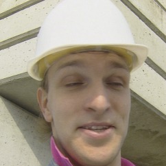
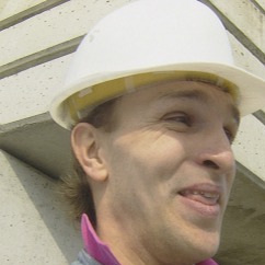
Fig. 2: Data set #2 : first and last frames of the “foreman” sequence.

• A real sample of the standard “foreman” video. In our simulations, we focus on a region of interest of $256\times 256$ pixels and on the 10 first images. The first and last images of this data set are displayed in Fig. 2. In the following, we will refer to this sequence as data set #2.

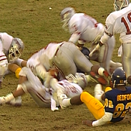
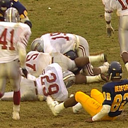
Fig. 3: Data set #3: first and last frames of the “football” sequences.

• A real sample of the challenging “football” video¹², which exhibits non-homogeneous and large displacements, as well as multiple occlusions. In our simulations, we focus on a region of interest of $256\times 256$ pixels and on the 10 first images. The first and last images of this data set are displayed in Fig. 3. In the following, we will refer to this sequence as data set #3.
  

The images of these sequences are composed of three spectral bands, each one is coded in 8 bits. We create the LR images by applying function $\mathcal{H}$ on these sequences. This function first filters the discrete signal by a Gaussian kernel of standard deviation equal to 1.12 and then down-samples the result by a factor of 2, see [9].

5.4 Evaluation Procedure

The performance of the algorithms is assessed in terms of reconstruction of the super-resolved image and estimation of the motion field. We describe the figures of merit used in our assessments hereafter. Let $\{\hat{\mathbf{x}}_{t}\}_{t=0}^{T}$ (resp. $\{\hat{\mathbf{d}}_{t}\}_{t=1}^{T}$) denote the estimated image sequence (resp. displacements) and $\{\mathbf{x}_{t}^{true}\}_{t=0}^{T}$ (resp. $\{\mathbf{d}_{t}^{true}\}_{t=1}^{T}$) the corresponding ground truth. Standard criteria [38] to measure the image sequence reconstruction accuracy are the peak-to-signal ratio (PSNR) at time $t$:

$$\text{PSNR}(t)=20\log_{10}\frac{n\|\mathbf{x}_{t}^{true}\|_{\infty}}{\|\mathbf{x}_{t}^{true}-\hat{\mathbf{x}}_{t}\|_{2}},$$

and the correlation coefficient (CC) at time $t$:

$$\text{CC}(t)=\frac{(\mathbf{x}_{t}^{true}-\mu_{\mathbf{x}_{t}^{true}})^{*}(\hat{\mathbf{x}}_{t}-\mu_{\hat{\mathbf{x}}_{t}})}{\|\mathbf{x}_{t}^{true}-\mu_{\mathbf{x}_{t}^{true}}\|_{2}\|\hat{\mathbf{x}}_{t}-\mu_{\hat{\mathbf{x}}_{t}}\|_{2}},$$

where we have denoted the arithmetic mean of vector $\hat{\mathbf{x}}_{t}$ and $\mathbf{x}_{t}^{true}$ by $\mu_{\hat{\mathbf{x}}_{t}}$ and $\mu_{\mathbf{x}_{t}^{true}}$. We evaluate the accuracy of the estimated motion fields with the time-averaged Mean End Point Error (MEPE):

$$\text{MEPE}=\frac{1}{nT}\sum_{t=1}^{T}\|\mathbf{d}_{t}^{true}-\hat{\mathbf{d}}_{t}\|_{1},$$

and the time-averaged Mean Barron Angular Error (MBAE) in degrees [5]:

$$\text{MBAE}=\frac{1}{nT}\sum_{t=1}^{T}\sum_{s=1}^{n}\text{arcos}\left(\frac{1+\mathbf{d}_{t}^{true}(s)\hat{\mathbf{d}}_{t}(s)+\mathbf{d}_{t}^{true}(s+n)\hat{\mathbf{d}}_{t}(s+n)}{\sqrt{(1+\hat{\mathbf{d}}_{t}(s)^{2}+\hat{\mathbf{d}}_{t}(s+n)^{2})\;(1+\mathbf{d}^{true}_{t}(s)^{2}+\mathbf{d}^{true}_{t}(s+n)^{2})}}\right),$$

where we have adopted the convention that the two $n$-dimensional components of motion have been sorted one after the other in vectors $\hat{\mathbf{d}}_{t}$ and $\mathbf{d}_{t}^{true}$.

In order to compare the different algorithms (algorithm [49] does not support large images and exclude pixels at the image border), the criteria PSNR and CC are evaluated on a spatial window of size of $240\times 240$ cropped in the image sequences.

5.5 Results and Discussion

	PSNR($t$)			CC($t$)
	set # 1	set # 2	set # 3	set # 1	set # 2	set # 3
	$t$=5	$t$=7	$t$=7	$t$=5	$t$=7	$t$=7
Nearest neighbor	27.236	22.639	22.656	0.9771	0.9648	0.9556
Lanczos interpolation [52]	27.845	24.571	23.040	0.9800	0.9775	0.9579
Single-frame SR [43]	28.359	32.518	23.971	0.9815	0.9949	0.9684
Kernel-regression SR [49, 48]	28.944	33.275	23.394	0.9838	0.9957	0.9643
Multi-frame SR [37]	29.935	32.295	21.948	0.9844	0.9939	0.9491
Proposed (optic-flow init. [61])	30.634	35.027	25.007	0.9868	0.9969	0.9750
Proposed (optic-flow init. [57])	30.790	34.305	25.302	0.9872	0.9963	0.9767

Table 2: Accuracy of super-resolved image estimates in terms of PSNR and CC at time $t$.

Table 2 presents the accuracy of the different algorithms in terms of PSNR and CC. We evaluated these criteria at $t=5$ for data set #1 and at $t=7$ for data sets #2 and #3. We first note that our SR method yields better figures of merit than the other methods for the different data sets of the benchmark. It improves slightly the CC and substantially the PSNR (more than a unit) for each data-set configuration. Second, the estimates released by the proposed approach seem to achieve a good quality level irrespective of the considered data set: on the contrary, the multi-frame SR algorithm [37] performs fairly well on data set #1 but its performance collapses on data set #3; the kernel-regression SR algorithm [49, 48] obtains good results for data set #2 while yielding only a slight increase of the accuracy with respect to a Lanczos interpolation on data set #3; the single-frame SR algorithm [43] has a good behavior for data set #3 but is less competitive for data set #1. Third, the performance of our algorithm seems to be comparable for different motion initializations, in particular for initial motion fields obtained from the optic-flow algorithms of [57] or [61].

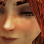
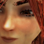
Fig. 4: “Single-image” SR estimates for data set #1. Details of the SR images obtained with nearest neighbor strategy ($1$-st row), Lanczos interpolation ($2$-nd row) and the learning algorithm proposed in [43] ($3$-rd row).

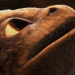
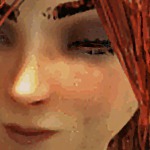
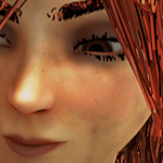
Fig. 5: Multi-frame and sequential SR estimates for data set #1. Details of the SR images obtained with the multi-frames algorithms of [49, 48] ($1$-st row) or [37] ($2$-nd row), and with the proposed sequential algorithm ($3$-rd row) in comparison to ground truth ($4$-th row). Initialization of our algorithm relies on the optic-flow method [57].

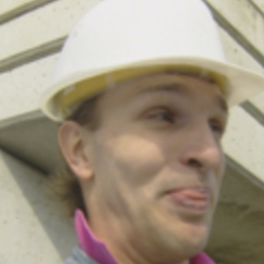
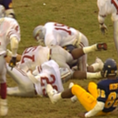
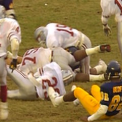
Fig. 6: “Single-image” SR estimates for data set #2 and #3. SR images and details obtained with nearest neighbor strategy ($1$-st row), Lanczos interpolation ($2$-nd row) and the learning algorithm of [43] ($3$-rd row).

The improvement brought by the proposed method can also be seen by a visual inspection of the reconstructed images in Fig. 4, 5, 6 and 7. We can first underline the enhancement provided by the inclusion of some motion information in the SR reconstruction process by comparing the estimates released by the “single-frame” and the “multi-frame”/“sequential” algorithms. In Fig. 4 and 6, one can notice that the estimated contours and the texture are over-smoothed if no motion information is included. This is for example visible by inspecting the fuzzy girl’s eyebrow or the smoothed scales of the little dragon in Fig. 4, distinguishing the tongue of the foreman or analyzing the texture of the grass field of the football game in Fig. 6. In comparison, our algorithm enhances the reconstruction accuracy of these details as visible in Fig. 5 and 7. The drawback of including motion is that, as it can be noticed for the little dragon, errors in motion discontinuity estimation may induce imprecision on the contours and lead to some undesirable oscillations.

Although not as accurate as the proposed method, we note the good performance of the single-frame SR algorithm proposed in [43]. Clearly, it is competitive with other state-of-the-art approaches exploiting motion information. This is probably due to the relevance of the sparse prior employed by the single-frame SR algorithm [43]. This is particularly striking when the motion in the video is too difficult to exploit by the multi-frame or kernel-regression SR algorithms, as shown for the challenging football sequence in Fig. 6 and 7. Let us also mention that results obtained with a kernel-regression SR strategy reveal a slight enhancement in comparison to standard spatial interpolation techniques, which is probably induced by the implicit introduction of the motion information via the modeling of the local spatio-temporal structures of the sequence.

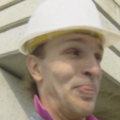
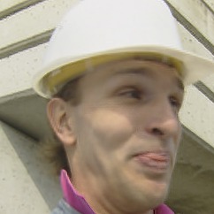
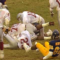
Fig. 7: Multi-frame or sequential SR estimates for data sets #2 and #3. SR images and details obtained with the multi-frame algorithms of [49, 48] ($1$-st row) or [37] ($2$-nd row), and with the proposed sequential algorithm ($3$-rd row) in comparison to ground truth ($4$-th row). Initialization of our algorithm relies on the optic-flow method [57].

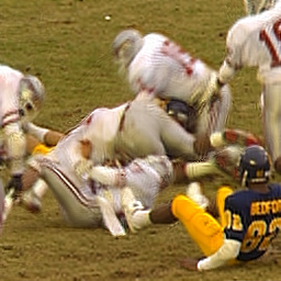
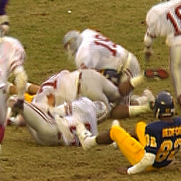
PSNR=26.989	PSNR=26.743	PSNR=26.560

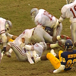
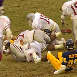
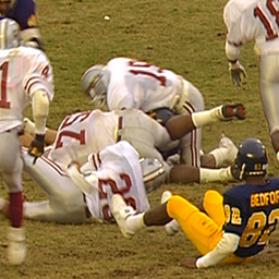
Fig. 9: Reconstruction of three super-resolved images $\mathbf{x}_{t}$ ($3$-rd row), optic-flow fields $\mathbf{d}_{t}$ ($1$-st row) and warping errors $\boldsymbol{\epsilon}_{t}$ ($2$-nd row) for data set #3 corresponding to $t=3$ (left) $t=5$ (middle) and $t=7$ (right). True images ($4$-th row) and associated PSNR (computed without quantification of the estimates and including the image borders) are displayed below. Initialization of our algorithm relies on the optic-flow method [57].

Our experiments also emphasize several examples where a sequential SR setup can solve some reconstruction ambiguities which can be difficult to treat in a multi-frame framework. In Fig. 5 and 7, some erroneous reconstructions, which do not appear in the proposed method, can be noticed in the multi-frame estimates: for example, artefacts in the girl’s eye in Fig. 5, deformations of the foreman’s tongue and the fuzziness of the stripes of the football player’s trousers in Fig. 7. Indeed, matching all the images of the sequence with a reference frame is often a more difficult task than estimating motions between consecutive frames. In the former situation, motion estimation has to deal with large displacements between distant frames whereas, in the latter setup, the problem simplifies into the estimation of a succession of small displacements. In other words, a SR multi-frame setup will try to match images of the sequence which could apparently seem independent, with the potential drawback of estimating erroneous structures. On the other hand, a SR sequential setup propagates information through consecutive frames and may better succeed in modeling the overall dependences in the image sequence. One could nevertheless argue that the estimation of inter-frame motions could also lead to error propagation if the motion estimates are inaccurate. This is not what we observed in our simulations: motion errors are usually absorbed by the error terms $\boldsymbol{\epsilon}_{t}$ (which increase in the region where the motion is badly estimated). This is illustrated in Fig. 9: we observe that $\boldsymbol{\epsilon}_{t}$ may be large on the contours of the characters (where the quality of the motion estimation is typically low) but the PSNR is nevertheless stable across the reconstructed image sequence. Therefore, as observed from our simulations, a sequential SR approach is usually better conditioned to deal with videos such as data sets #1 and #3, which exhibit large displacements and/or occlusions.

	LR estimate		SR estimate
	MEPE	MBAE	MEPE	MBAE
Zach et al., 2007 [61].	1.319	24.988	1.302	24.975
Xu et al., 2012 [57].	1.342	25.592	1.320	25.545

Table 3: Accuracy of low-resolved or super-resolved optic-flow estimates in terms of MEPE and MBAE, with respect to the motion initialization algorithm.

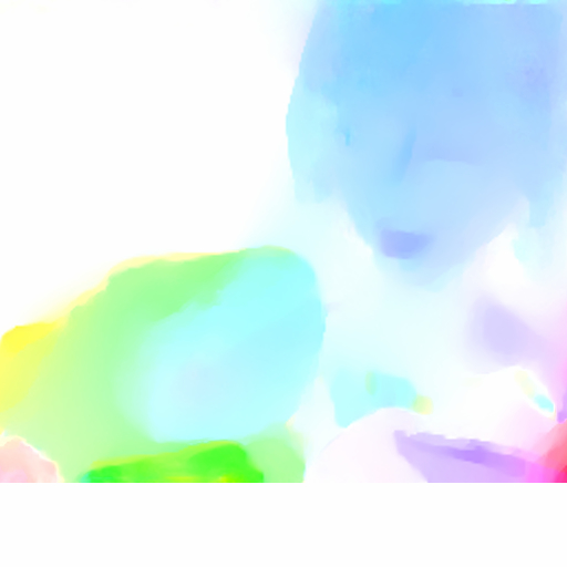
Fig. 8: Optic-flow SR estimates. Motion field estimated from low-resolved images of data set #1 at initial time. Top: estimates for state-of-the-art algorithms [57] (left) and [61] (right). Middle: estimates with the proposed SR algorithm initialized with [57] (left) or [61] (right). Bottom: ground truth and associated colormap.

Finally, let us notice that there is a positive interaction between the estimation of the motion fields and the HR images: intuitively, it is clear that a good estimation of the HR image sequence will improve the quality of the estimated motion fields; similarly, a good estimation of the super-resolved motion fields will enhance the accuracy of the estimated image sequence. Although this positive interaction is difficult to ensure from a theoretical side, we have often observed it in practice. We illustrate in Table 3 and Fig. 8 the benefit of refining the motion estimation through our iterative procedure for the synthetic data set #1, independently of the initial motion estimate. In Table 3, we can notice a slight gain in terms of MBAE and MEPE in comparison to a direct estimation of the motion from the LR observations with the methods presented in [57] or [61] (which serve as initializations for our algorithm, see section 5.1). More interestingly, we note in Fig. 8 that the motion field released by the proposed approach exhibits sharper discontinuities than those output by [57] or [61].

6 Conclusion

We have presented a new methodology to solve video SR problems, i.e., to reconstruct a HR image sequence from LR observations. The HR sequence is entirely described by a parametric non-linear sequential model, which connects the different images of the sequence. It is parametrized by a final condition, a sequence of non-global displacement fields and a sequence of additive noises. In order to compensate for the ill-posedness of the video SR problem, we considered priors enforcing some forms of sparsity on the unknown parameters of the system. The joint estimation of the final condition, the displacement and the noise sequences was expressed as a constrained minimization problem which, in the general case, is high-dimensional, non-differentiable and non-convex. We provided elementary building blocks to tackle each of these difficulties, and, by gathering them, designed a convergent optimization algorithm enjoying a complexity (per iteration) linear in the problem dimensions. Our numerical simulations on several video benchmarks show that the proposed SR method is competitive with state-of the-art. In particular, the gain appears to be particularly important for videos involving complex motions with large amplitudes and occlusions.

Appendix A Proof of (10)-(12)

The proof of this specific backward optimal control solution follows the sketch of the demonstration for the more standard forward problem presented in [6]. We will focus on the following optimization problem:

$$\operatorname*{arg\,min}_{(\boldsymbol{\epsilon},\mathbf{d},\mathbf{c})}\mathcal{T}(\mathbf{x}=\mathcal{Q}(\boldsymbol{\epsilon},\mathbf{d},\mathbf{c}),\boldsymbol{\epsilon},\mathbf{d},\mathbf{c}),$$ (44)

where $\mathcal{T}$ denotes some objective function to be defined below. We recall that, given ($\boldsymbol{\epsilon},\mathbf{d}$, $\mathbf{c})$, the function $\mathcal{Q}(\boldsymbol{\epsilon},\mathbf{d},\mathbf{c})$ determines a unique vector $\mathbf{x}=\mathcal{Q}(\boldsymbol{\epsilon},\mathbf{d},\mathbf{c})$ satisfying the constraints in (6), see section 4.1. In this appendix, we will use the following short-hand notation for the constraints in (6):

$$\left\{\begin{aligned} &\mathbf{x}_{t}=\mathcal{F}_{t}(\mathbf{x}_{t+1},\boldsymbol{\epsilon}_{t+1},\mathbf{d}_{t+1}),&\hskip 5.69046pt0\leq t\leq T-1,\\ &\mathbf{x}_{T}=\mathbf{D}\mathbf{c},&\hskip 5.69046pt\end{aligned}\right.$$ (45)

with $\mathcal{F}_{t}(\mathbf{x}_{t+1},\boldsymbol{\epsilon}_{t+1},\mathbf{d}_{t+1})\triangleq\mathcal{P}(\mathbf{x}_{t+1},\mathbf{d}_{t+1})+\boldsymbol{\epsilon}_{t+1}$. We will also alleviate the notation for the constraint $\mathbf{x}=\mathcal{Q}(\boldsymbol{\epsilon},\mathbf{d},\mathbf{c})$ by denoting this vector simply by $\mathbf{x}$. Therefore, $\mathbf{x}$ should be understood as a function of $\boldsymbol{\epsilon},\mathbf{d},\mathbf{c}$ and no longer as an independent variable.

The proof of (10)-(12) is made of two different parts, in which we study different instances of optimization problem (44). In a first step, we will consider an objective function only depending on the initial state:

$$\mathcal{T}(\mathbf{x},\boldsymbol{\epsilon},\mathbf{d},\mathbf{c})\triangleq\mathcal{G}_{0}(\mathbf{x}_{0}).$$ (46)

Then, in a second step, we will come back to the more general problem (7), i.e., an optimization problem where the objective function $\mathcal{T}$ will match the cost function, $\mathcal{J}$, given in (8):

$$\mathcal{T}(\mathbf{x},\boldsymbol{\epsilon},\mathbf{d},\mathbf{c})\triangleq\mathcal{G}_{0}(\mathbf{x}_{0})+\sum_{t={1}}^{T-1}\mathcal{G}_{t}(\mathbf{x}_{t},\boldsymbol{\epsilon}_{t},\mathbf{d}_{t})+\mathcal{G}_{T}(\mathbf{x}_{T},\boldsymbol{\epsilon}_{T},\mathbf{d}_{T},\mathbf{c})\triangleq\mathcal{J}(\mathbf{x},\boldsymbol{\epsilon},\mathbf{d},\mathbf{c}).$$ (47)

First Part of the Proof.  We begin by considering problem (44) with the objective function (46). By the chain rule of derivation applied to (45) at some point in the set

$$\left\{(\mathbf{x}^{\prime},\boldsymbol{\epsilon}^{\prime},\mathbf{d}^{\prime},\mathbf{c}^{\prime})\left|\begin{aligned} \mathbf{x}^{\prime}_{t}=\mathcal{F}_{t}(\mathbf{x}^{\prime}_{t+1},\boldsymbol{\epsilon}^{\prime}_{t+1},\mathbf{d}^{\prime}_{t+1}),&\hskip 5.69046pt0\leq t\leq T-1\\ \;\;\mathbf{x}^{\prime}_{T}=\mathbf{D}\mathbf{c}^{\prime}&\hskip 5.69046pt\end{aligned}\right.\right\},$$ (48)

we can decompose the gradients into the products:

$$\left\{\begin{aligned} \nabla_{\boldsymbol{\epsilon}_{t}}\mathcal{T}(\mathbf{x}^{\prime},\boldsymbol{\epsilon}^{\prime},\mathbf{d}^{\prime},\mathbf{c}^{\prime})&=\nabla_{\boldsymbol{\epsilon}_{t}}\mathcal{F}_{t-1}^{*}(\mathbf{x}_{t}^{\prime},\boldsymbol{\epsilon}_{t}^{\prime},\mathbf{d}_{t}^{\prime})\,\nabla_{\mathbf{x}_{t-1}}\mathcal{F}_{t-2}^{*}\,\cdots\nabla_{\mathbf{x}_{2}}\mathcal{F}_{1}^{*}\,\nabla_{\mathbf{x}_{1}}\mathcal{F}_{0}^{*}\,\nabla_{\mathbf{x}_{0}}\mathcal{G}_{0}(\mathbf{x}_{0}^{\prime}),\\ \nabla_{\mathbf{d}_{t}}\mathcal{T}(\mathbf{x}^{\prime},\boldsymbol{\epsilon}^{\prime},\mathbf{d}^{\prime},\mathbf{c}^{\prime})&=\nabla_{\mathbf{d}_{t}}\mathcal{F}_{t-1}^{*}(\mathbf{x}_{t}^{\prime},\boldsymbol{\epsilon}_{t}^{\prime},\mathbf{d}_{t}^{\prime})\,\nabla_{\mathbf{x}_{t-1}}\mathcal{F}_{t-2}^{*}\,\cdots\nabla_{\mathbf{x}_{2}}\mathcal{F}_{1}^{*}\,\nabla_{\mathbf{x}_{1}}\mathcal{F}_{0}^{*}\,\nabla_{\mathbf{x}_{0}}\mathcal{G}_{0}(\mathbf{x}_{0}^{\prime}),\\ \nabla_{\mathbf{c}}\mathcal{T}(\mathbf{x}^{\prime},\boldsymbol{\epsilon}^{\prime},\mathbf{d}^{\prime},\mathbf{c}^{\prime})&=\mathbf{D}^{*}\nabla_{\mathbf{x}_{T}}\mathcal{F}_{T-1}^{*}\,\cdots\nabla_{\mathbf{x}_{2}}\mathcal{F}_{1}^{*}\,\nabla_{\mathbf{x}_{1}}\mathcal{F}_{0}^{*}\,\nabla_{\mathbf{x}_{0}}\mathcal{G}_{0}(\mathbf{x}_{0}^{\prime}),\end{aligned}\right.$$ (49)

where we recall that $\nabla_{\mathbf{x}_{t}}\mathcal{F}_{t-1}$ denotes the Jacobian matrice of $\mathcal{F}_{t-1}$ with respect to function $\mathbf{x}_{t}$ evaluated at $(\mathbf{x}_{t}^{\prime},\boldsymbol{\epsilon}_{t}^{\prime},\mathbf{d}_{t}^{\prime})$ and $\nabla_{\mathbf{x}_{t}}\mathcal{F}_{t-1}^{*}$ its transpose. We can rewrite gradients in (49) in order to exhibit their recursive structures. By defining the forward recursion

$$\left\{\begin{aligned} &\boldsymbol{\zeta}_{0}=\nabla_{\mathbf{x}_{0}}\mathcal{G}_{0}(\mathbf{x}_{0}^{\prime}),\\ &\boldsymbol{\zeta}_{t}=\nabla_{\mathbf{x}_{t}}\mathcal{F}_{t-1}^{*}\boldsymbol{\zeta}_{t-1},\hskip 8.5359pt1\leq t\leq T,\end{aligned}\right.$$ (50)

we obtain the following rewriting:

$$\left\{\begin{aligned} &\nabla_{\boldsymbol{\epsilon}_{t}}\mathcal{T}(\mathbf{x}^{\prime},\boldsymbol{\epsilon}^{\prime},\mathbf{d}^{\prime},\mathbf{c}^{\prime})=\nabla_{\boldsymbol{\epsilon}_{t}}\mathcal{F}_{t-1}^{*}(\mathbf{x}_{t}^{\prime},\boldsymbol{\epsilon}_{t}^{\prime},\mathbf{d}_{t}^{\prime})\boldsymbol{\zeta}_{t-1},\hskip 8.5359pt1\leq t\leq T,\\ &\nabla_{\mathbf{d}_{t}}\mathcal{T}(\mathbf{x}^{\prime},\boldsymbol{\epsilon}^{\prime},\mathbf{d}^{\prime},\mathbf{c}^{\prime})=\nabla_{\mathbf{d}_{t}}\mathcal{F}_{t-1}^{*}(\mathbf{x}_{t}^{\prime},\boldsymbol{\epsilon}_{t}^{\prime},\mathbf{d}_{t}^{\prime})\boldsymbol{\zeta}_{t-1},\hskip 8.5359pt1\leq t\leq T,\\ &\nabla_{\mathbf{c}}\mathcal{T}(\mathbf{x}^{\prime},\boldsymbol{\epsilon}^{\prime},\mathbf{d}^{\prime},\mathbf{c}^{\prime})=\mathbf{D}^{*}\boldsymbol{\zeta}_{T}.\\ \end{aligned}\right.\\$$ (51)

Second Part of the Proof.  We now consider problem (44) with objective function (47). By making a change of variables, we want to obtain a rewriting of function (47) with a structure analogous to (46), so that the gradients are given by a recursion of the form (50)-(51). In other words, by making some change of variables we intend to rewrite the sum of functions in (47) as a unique function depending solely on an “initial state”. In order to do so, let us define variables $\boldsymbol{\kappa}_{i}$’s recursively as follows:

$$\left\{\begin{aligned} &\boldsymbol{\kappa}_{T}=0,\\ &\boldsymbol{\kappa}_{T-1}(\mathbf{x}_{T},\boldsymbol{\epsilon}_{T},\mathbf{d}_{T},\mathbf{c})=\boldsymbol{\kappa}_{T}+\mathcal{G}_{T}(\mathbf{x}_{T},\boldsymbol{\epsilon}_{T},\mathbf{d}_{T},\mathbf{c}),\\ &\boldsymbol{\kappa}_{t-1}(\mathbf{x}_{t},\boldsymbol{\epsilon}_{t},\mathbf{d}_{t},\mathbf{c})=\boldsymbol{\kappa}_{t}+\mathcal{G}_{t}(\mathbf{x}_{t},\boldsymbol{\epsilon}_{t},\mathbf{d}_{t}),\hskip 8.5359ptT-1\geq t\geq 1.\end{aligned}\right.$$

We then obtain that

$$\boldsymbol{\kappa}_{0}(\mathbf{x},\boldsymbol{\epsilon},\mathbf{d},\mathbf{c})=\sum_{t={1}}^{T-1}\mathcal{G}_{t}(\mathbf{x}_{t},\boldsymbol{\epsilon}_{t},\mathbf{d}_{t})+\mathcal{G}_{T}(\mathbf{x}_{T},\boldsymbol{\epsilon}_{T},\mathbf{d}_{T},\mathbf{c}),$$

and the objective function $\mathcal{T}$ given in (47) can be rewritten as

$$\mathcal{T}(\mathbf{x},\boldsymbol{\epsilon},\mathbf{d},\mathbf{c})=\boldsymbol{\kappa}_{0}(\mathbf{x},\boldsymbol{\epsilon},\mathbf{d},\mathbf{c})+\mathcal{G}_{0}(\mathbf{x}_{0}).$$ (52)

Considering the following change of variables $\tilde{\mathbf{x}}_{t}\triangleq\begin{pmatrix}\mathbf{x}_{t}\\ \boldsymbol{\kappa}_{t}\end{pmatrix}$, we then have that the right-hand side of (52) can be rewritten as a function of $\tilde{\mathbf{x}}_{0}$ only. In the sequel, we will use the following specific notation to emphasize this fact:

$$\mathcal{\tilde{G}}_{0}(\tilde{\mathbf{x}}_{0})=\boldsymbol{\kappa}_{0}+\mathcal{G}_{0}(\mathbf{x}_{0}).$$ (53)

Moreover, it is easy to see that functions $\tilde{\mathbf{x}}_{t}$’s satisfy the following backward recursion:

$$\left\{\begin{aligned} &\tilde{\mathbf{x}}_{t}=\mathcal{\tilde{F}}_{t}(\tilde{\mathbf{x}}_{t+1},\boldsymbol{\epsilon}_{t+1},\mathbf{d}_{t+1}),\hskip 8.5359ptT-1\geq t\geq 0,\\ &\tilde{\mathbf{x}}_{T}=\mathcal{\tilde{F}}_{T}(\boldsymbol{\epsilon}_{T},\mathbf{d}_{T},\mathbf{c}),\\ \end{aligned}\right.$$ (54)

where

$$\mathcal{\tilde{F}}_{t}(\tilde{\mathbf{x}}_{t+1},\boldsymbol{\epsilon}_{t+1},\mathbf{d}_{t+1}) =\begin{pmatrix}\mathcal{F}_{t}(\mathbf{x}_{t+1},\boldsymbol{\epsilon}_{t+1},\mathbf{d}_{t+1})\\ \boldsymbol{\kappa}_{t+1}+\mathcal{G}_{t+1}(\mathbf{x}_{t+1},\boldsymbol{\epsilon}_{t+1},\mathbf{d}_{t+1})\end{pmatrix},$$

$$\tilde{\mathcal{F}}_{T}(\boldsymbol{\epsilon}_{T},\mathbf{d}_{T},\mathbf{c}) =\begin{pmatrix}\mathbf{D}\mathbf{c}\\ \mathcal{G}_{T}(\mathbf{D}\mathbf{c},\boldsymbol{\epsilon}_{T},\mathbf{d}_{T},\mathbf{c})\end{pmatrix}.$$

We remark that the cost function (53), recursion (54) and the set

$$\left\{(\tilde{\mathbf{x}}^{\prime},\boldsymbol{\epsilon}^{\prime},\mathbf{d}^{\prime},\mathbf{c}^{\prime})\left|\begin{aligned} \tilde{\mathbf{x}}^{\prime}_{t}=\mathcal{\tilde{F}}_{t}(\tilde{\mathbf{x}}^{\prime}_{t+1},\boldsymbol{\epsilon}^{\prime}_{t+1},\mathbf{d}^{\prime}_{t+1}),&\hskip 5.69046pt0\leq t\leq T-1\\ \;\;\tilde{\mathbf{x}}^{\prime}_{T}=\mathcal{\tilde{F}}_{T}(\boldsymbol{\epsilon}_{T}^{\prime},\mathbf{d}_{T}^{\prime},\mathbf{c}^{\prime})&\hskip 5.69046pt\end{aligned}\right.\right\},$$ (55)

have respectively the same structure as (46), (45) and (48). We can then apply the result obtained previously and get the gradients of $\mathcal{T}$ using the same reasoning as the one made to derive (50)-(51). More specifically, let $(\tilde{\mathbf{x}}^{\prime},\boldsymbol{\epsilon}^{\prime},\mathbf{d}^{\prime},\mathbf{c}^{\prime})$ be some point in (55), and let $\tilde{\boldsymbol{\zeta}}_{t}$ be an “adjoint” variable verifying:

$$\left\{\begin{aligned} &\tilde{\boldsymbol{\zeta}}_{0}=\nabla_{\tilde{\mathbf{x}}_{0}}\mathcal{\tilde{G}}_{0}(\tilde{\mathbf{x}}_{0}^{\prime}),\\ &\tilde{\boldsymbol{\zeta}}_{t}=\nabla_{\tilde{\mathbf{x}}_{t}}\mathcal{\tilde{F}}_{t-1}^{*}\tilde{\boldsymbol{\zeta}}_{t-1},\hskip 8.5359pt1\leq t\leq T,\end{aligned}\right.$$ (56)

where the Jacobian matrix of $\mathcal{\tilde{F}}_{t-1}$ evaluated at some point $(\tilde{\mathbf{x}}_{t}^{\prime},\boldsymbol{\epsilon}_{t}^{\prime},\mathbf{d}_{t}^{\prime})$ is denoted $\nabla_{\tilde{\mathbf{x}}_{t}}\mathcal{\tilde{F}}_{t-1}$. Using (51), we obtain the following expressions:

$$\left\{\begin{aligned} &\nabla_{\mathbf{d}_{t}}\mathcal{T}(\tilde{\mathbf{x}}^{\prime},\boldsymbol{\epsilon}^{\prime},\mathbf{d}^{\prime},\mathbf{c}^{\prime})=\nabla_{\mathbf{d}_{t}}\mathcal{\tilde{F}}_{t-1}^{*}(\tilde{\mathbf{x}}_{t}^{\prime},\boldsymbol{\epsilon}_{t}^{\prime},\mathbf{d}_{t}^{\prime})\tilde{\boldsymbol{\zeta}}_{t-1},\hskip 8.5359pt1\leq t\leq T,\\ &\nabla_{\boldsymbol{\epsilon}_{t}}\mathcal{T}(\tilde{\mathbf{x}}^{\prime},\boldsymbol{\epsilon}^{\prime},\mathbf{d}^{\prime},\mathbf{c}^{\prime})=\nabla_{\boldsymbol{\epsilon}_{t}}\mathcal{\tilde{F}}_{t-1}^{*}(\tilde{\mathbf{x}}_{t}^{\prime},\boldsymbol{\epsilon}_{t}^{\prime},\mathbf{d}_{t}^{\prime})\tilde{\boldsymbol{\zeta}}_{t-1},\hskip 8.5359pt1\leq t\leq T,\\ &\nabla_{\mathbf{c}}\mathcal{T}(\tilde{\mathbf{x}}^{\prime},\boldsymbol{\epsilon}^{\prime},\mathbf{d}^{\prime},\mathbf{c}^{\prime})=\nabla_{\mathbf{c}}\mathcal{\tilde{F}}_{T}^{*}(\boldsymbol{\epsilon}_{T}^{\prime},\mathbf{d}_{T}^{\prime},\mathbf{c}^{\prime})\tilde{\boldsymbol{\zeta}}_{T}.\end{aligned}\right.$$

To finalize the proof, we re-express recursion (56) by developing it with respect to the two different components of the adjoint variable $\tilde{\boldsymbol{\zeta}}_{t}\triangleq\begin{pmatrix}\boldsymbol{\zeta}_{t}\\ \omega_{t}\end{pmatrix}$, where the $\boldsymbol{\zeta}_{t}$’s have the dimension of $\mathbf{x}_{t}$’s and $\omega_{t}$’s are scalars. Particularizing the first equation in (56) by taking (53) into account, we obtain

$$\begin{pmatrix}\boldsymbol{\zeta}_{0}\\ \omega_{0}\end{pmatrix} =\begin{pmatrix}\nabla_{\mathbf{x}_{0}}\mathcal{\tilde{G}}_{0}(\tilde{\mathbf{x}}_{0}^{\prime})\\ \nabla_{\boldsymbol{\kappa}_{0}}\mathcal{\tilde{G}}_{0}(\tilde{\mathbf{x}}_{0}^{\prime})\end{pmatrix}=\begin{pmatrix}\nabla\mathcal{G}_{0}(\mathbf{x}_{0}^{\prime})\\ 1\end{pmatrix}.$$ (57)

Moreover, using the definition of $\tilde{\mathcal{F}}_{t}$, the second equation in (56) leads to

$$\begin{pmatrix}\boldsymbol{\zeta}_{t}\\ \omega_{t}\end{pmatrix} =\begin{pmatrix}\nabla_{\mathbf{x}_{t}}\mathcal{F}_{t-1}^{*}&\nabla_{\mathbf{x}_{t}}\mathcal{G}_{t}(\mathbf{x}_{t}^{\prime},\boldsymbol{\epsilon}_{t}^{\prime},\mathbf{d}_{t}^{\prime})\\ 0&1\end{pmatrix}\begin{pmatrix}\boldsymbol{\zeta}_{t-1}\\ \omega_{t-1}\end{pmatrix},\quad 1\leq t\leq T-1,$$ (58)

$$\begin{pmatrix}\boldsymbol{\zeta}_{T}\\ \omega_{T}\end{pmatrix} =\begin{pmatrix}\nabla_{\mathbf{x}_{T}}\mathcal{F}_{T-1}^{*}&\nabla_{\mathbf{x}_{T}}\mathcal{G}_{T}(\mathbf{x}_{T}^{\prime},\boldsymbol{\epsilon}_{T}^{\prime},\mathbf{d}_{T}^{\prime},\mathbf{c}^{\prime})\\ 0&1\end{pmatrix}\begin{pmatrix}\boldsymbol{\zeta}_{T-1}\\ \omega_{T-1}\end{pmatrix}.$$ (59)

Equations (57)-(59) imply that $\omega_{t}=1$ $\forall t$; moreover, the recursion in $\boldsymbol{\zeta}_{t}$ is equivalent to (12).

Appendix B The Alternating Direction Method of Multipliers

The alternating direction method of multipliers (ADMM) focusses on the following type of optimization problems:

$$\min_{\boldsymbol{z}_{1}\in\Xi_{1},\boldsymbol{z}_{2}\in\Xi_{1}}\mathcal{G}_{1}(\boldsymbol{z}_{1})+\mathcal{G}_{2}(\boldsymbol{z}_{2}),\quad\mbox{ s.t. $\mathbf{A}\boldsymbol{z}_{1}+\mathbf{B}\boldsymbol{z}_{2}=\mathbf{0}_{r}$},$$ (60)

where $\mathbf{A}\in\mathds{R}^{r\times n_{1}}$, $\mathbf{B}\in\mathds{R}^{r\times n_{2}}$, $\mathcal{G}_{1}:\mathds{R}^{n_{1}}\rightarrow\mathds{R}$, $\mathcal{G}_{2}:\mathds{R}^{n_{2}}\rightarrow\mathds{R}$ are closed, proper and convex functions, and $\Xi_{1}$, $\Xi_{2}$ are non-empty convex sets. We note that the conditions on $\mathcal{G}_{1}$ and $\mathcal{G}_{2}$ are pretty mild; in particular, $\mathcal{G}_{1}$ and $\mathcal{G}_{2}$ are not required to be differentiable and can take on infinite values.

ADMM is an iterative procedure inspired by the well-known method of multipliers [6]. It searches for a minimizer of (60) by sequentially minimizing the corresponding augmented Lagrangian with respect to each primal variables $\boldsymbol{z}_{1}$ and $\boldsymbol{z}_{2}$, before updating a dual variable $\mathbf{u}\in\mathds{R}^{r}$. Formally, the ADMM recursions take the form:

$$\boldsymbol{z}_{1}^{(k+1)} =\operatorname*{arg\,min}_{\boldsymbol{z}_{1}\in\Xi_{1}}\mathcal{G}_{1}(\boldsymbol{z}_{1})+\frac{\rho}{2}\|\mathbf{A}\boldsymbol{z}_{1}+\mathbf{B}\boldsymbol{z}_{2}^{(k)}+\mathbf{u}^{(k)}\|^{2}_{2},$$ (61)

$$\boldsymbol{z}_{2}^{(k+1)} =\operatorname*{arg\,min}_{\boldsymbol{z}_{2}\in\Xi_{2}}\mathcal{G}_{2}(\boldsymbol{z}_{2})+\frac{\rho}{2}\|\mathbf{A}\boldsymbol{z}_{1}^{(k+1)}+\mathbf{B}\boldsymbol{z}_{2}+\mathbf{u}^{(k)}\|^{2}_{2},$$ (62)

$$\mathbf{u}^{(k+1)} =\mathbf{u}^{(k)}+\mathbf{A}\boldsymbol{z}_{1}^{(k+1)}+\mathbf{B}\boldsymbol{z}_{2}^{(k+1)},$$ (63)

for some $\rho>0$.

ADMM has recently sparked a surge of interest in the signal-processing community for several reasons. First, the conditions on $\mathcal{G}_{1}$ and $\mathcal{G}_{2}$ in (60) (i.e., closed, proper and convex) are mild and (60) therefore encompasses a large number of optimization problems as particular cases. Second, the ADMM recursion (61)-(63) converges to a solution of (60) under very general conditions, see [8, section 3.2]. Third, although ADMM is known to be slow to converge to a solution with high accuracy, it has been shown empirically that ADMM converges to modest accuracy in a few tens of iterations.

Appendix C Algorithm’s Details

C.1 First Building Block: Computation of (10)-(12)

In this appendix, we complement the exposition done in section 4.1 on the fast evaluation of gradient of cost function $\mathcal{J}(\boldsymbol{\epsilon},\mathbf{d},\mathbf{c})$ given in (8), particularized to the model parameters specified in section 5.1. First of all, we expose the particularization of recursions (10)-(12) to this setting. It is straightforward to see that it results in the following procedure:

• Compute sequence $\{\mathbf{x}_{t}^{\prime}\}_{t=0}^{T}$ by the backward recursion:
  $\left\{\begin{aligned} &\mathbf{x}_{T}^{\prime}=\mathbf{D}\mathbf{c}^{\prime},\\ &\mathbf{x}_{t}^{\prime}=\mathcal{P}(\mathbf{x}_{t+1}^{\prime},\mathbf{d}_{t+1}^{\prime})+\boldsymbol{\epsilon}_{t+1}^{\prime}.\\ \end{aligned}\right.\\$

• Compute sequence $\{\boldsymbol{\zeta}_{t}\}_{t=0}^{T}$ by the forward recursion:

  $\left\{\begin{aligned} &\boldsymbol{\zeta}_{0}=2\nabla_{\mathbf{x}_{0}}\mathcal{H}^{*}(\mathcal{H}(\mathbf{x}_{0}^{\prime})-\mathbf{y}_{0}),\\ &\boldsymbol{\zeta}_{t+1}=\nabla_{\mathbf{x}_{t+1}}\mathcal{P}^{*}(\mathbf{x}_{t+1}^{\prime},\mathbf{d}_{t+1}^{\prime})\boldsymbol{\zeta}_{t},+2\nabla_{\mathbf{x}_{t+1}}\mathcal{H}^{*}(\mathcal{H}(\mathbf{x}_{t+1}^{\prime})-\mathbf{y}_{t+1}).\end{aligned}\right.$

• Compute the gradients:
  $\left\{\begin{aligned} &\nabla_{\boldsymbol{\epsilon}_{t}}\mathcal{J}(\boldsymbol{\epsilon}^{\prime},\mathbf{d}^{\prime},\mathbf{c}^{\prime})=\boldsymbol{\zeta}_{t-1}+2\alpha_{1}\boldsymbol{\epsilon}_{t}^{\prime},\\ &\nabla_{\mathbf{d}_{t}}\mathcal{J}(\boldsymbol{\epsilon}^{\prime},\mathbf{d}^{\prime},\mathbf{c}^{\prime})=\mathbf{E}_{t}\boldsymbol{\zeta}_{t-1}+2\alpha_{2}\mathbf{W}_{t}\mathbf{G}\mathbf{G}^{*}\mathbf{d}_{t}^{\prime},\\ &\nabla_{\mathbf{c}}\mathcal{J}(\boldsymbol{\epsilon}^{\prime},\mathbf{d}^{\prime},\mathbf{c}^{\prime})=\mathbf{D}^{*}\boldsymbol{\zeta}_{T}+2\alpha_{3}\mathbf{c}^{\prime}\end{aligned}\right.\\$

where $\mathbf{W}_{t}\in\mathds{R}^{2n\times 2n}$ and $\mathbf{E}_{t}\in\mathds{R}^{2n\times n}$ are respectively diagonal and block-diagonal matrices which will be defined in the following. We detail hereafter the elements of the procedure which have not been fully described yet.

We begin by making some comments on the evaluation of the warping function $\mathcal{P}(\mathbf{x}_{t}^{\prime},\mathbf{d}_{t}^{\prime})$ and its Jacobian $\nabla_{\mathbf{x}_{t}}\mathcal{P}(\mathbf{x}_{t}^{\prime},\mathbf{d}_{t}^{\prime})$, which constitute the core of the recursion. We propose to use the family of bi-dimensional cubic cardinal splines $\{\psi_{i}\}_{i=1}^{n}$ for the representation (3). In practice, we compute an equivalent representation based on the family of bi-dimensional cubic B-splines functions $\{\phi_{i}\}_{i=1}^{n}$. Indeed, this representation presents some computational advantages because of the existence of fast B-splines transforms. The relation between cardinal cubic splines and cubic B-splines functions is given in [54]. This reference also provides details on the fast cubic B-splines transform by recursive filtering. Let matrix $\mathbf{C}^{*}=[\mathbf{c}_{1},...,\mathbf{c}_{n}]^{*}\in\mathds{R}^{n\times n}$ denote the direct B-spline transform of a discrete bi-dimensional signal, i.e., the transform computing from a discrete signal $\mathbf{x}_{t}$ its representation with spline coefficients $\mathbf{C}^{*}\mathbf{x}_{t}$. Rewritten (3) with cubic B-spline functions, we get:

$$\mathcal{P}_{s}(\mathbf{x}_{t},{\mathbf{d}_{t}}) =\sum_{i\in\vartheta(\chi(s)+\mathbf{d}_{t}({s}))}\mathbf{c}_{i}^{*}\mathbf{x}_{t}\,\phi_{i}(\chi(s)+\mathbf{d}_{t}(s)),$$ (64)

where $\vartheta(\chi(s)+\mathbf{d}_{t}({s}))$ denotes a subset of vector indices corresponding to the neighborhood of the spatial position $\chi(s)$ (which differs from the subset $\mathcal{V}$ previously defined in (3)). To simplify notations, we denote by $\mathcal{I}:\mathds{R}^{n}\times\mathds{R}^{2n}\to\mathds{R}^{n}$ the function taking as a first argument spline coefficients $\mathbf{C}^{*}\mathbf{x}_{t}$ and as a second argument a motion field $\mathbf{d}_{t}$, and whose $s$-th component is given by (64). Using this notation, (64) can be rewritten in the vectorial form

$$\mathcal{P}(\mathbf{x}_{t},{\mathbf{d}_{t}}) =\mathcal{I}(\mathbf{C}^{*}\mathbf{x}_{t},\mathbf{d}_{t}).$$

We denote by $\nabla\mathcal{I}(\mathbf{C}^{*}\mathbf{x}_{t},\mathbf{d}_{t})$ the Jacobian of function $\mathcal{I}$ at point $(\mathbf{C}^{*}\mathbf{x}_{t},\mathbf{d}_{t})$ with respect to its first argument, i.e., spline coefficients. Since function $\mathcal{I}$ is linear with respect to spline coefficients, the Jacobian is only dependent on the value of its second argument, i.e., $\mathbf{d}_{t}$. Therefore, we will adopt the notation $\nabla\mathcal{I}(\mathbf{d}_{t})$ in the sequel.

The complexity of evaluating both spline coefficients $\mathbf{C}^{*}\mathbf{x}_{t}$ and the interpolated function $\mathcal{I}$, scales linearly with the image dimension, i.e., $\mathcal{O}(n)$, thanks to the representation separability and to recursive linear filtering [54]. Multiplication with the Jacobian transpose

$$\nabla_{\mathbf{x}_{t}}\mathcal{P}^{*}(\mathbf{x}_{t+1},\mathbf{d}_{t+1})=\mathbf{C}\nabla\mathcal{I}^{*}(\mathbf{d}_{t+1}),$$

implies also a linear complexity: first, matrix $\mathbf{C}$ is symmetric so that it is identical to the direct B-spline transformation $\mathbf{C}^{*}$, computed by recursive linear filtering; second, the multiplication of the Jacobian transpose of function $\mathcal{I}$ with vector $\boldsymbol{\zeta}_{t}$ is equal to

$$\nabla\mathcal{I}^{*}(\mathbf{d}_{t})\boldsymbol{\zeta}_{t}(s)=\sum_{i|s\in\vartheta(\chi(i)+\mathbf{d}_{t}({i}))}\boldsymbol{\zeta}_{t}(i)\phi_{s}(\chi(i)+\mathbf{d}_{t}({i})).$$

Concerning the Jacobian transpose $\nabla_{\mathbf{x}_{t}}\mathcal{H}^{*}$, it is easy to see that this matrix is an up-sampling operation, inserting zeros, followed by the same low-pass filtering as in $\mathcal{H}$.

We continue by detailing matrices appearing in the last step of the procedure. First, we note that matrix $\mathbf{D}^{*}$ is simply the direct Real-valued Fast Curvelet Transform. This transform is, as well as its transpose $\mathbf{D}$, based on fast Fourier transforms, whose complexity scales in $\mathcal{O}(n\log n)$ [35]. Next, the two diagonals of the two-block matrix $\mathbf{E}_{t}$ are the two $n$-dimensional vectors $\partial_{s_{j}}\left(\mathcal{I}(\mathbf{C}^{*}\mathbf{x}_{t},\mathbf{d}_{t})\right)$ for $j=1,2$, where $s_{j}$ denotes the $j$-th spatial coordinate. We approach these partial derivatives by second-order centered finite differences. Then, the diagonal of matrix $\mathbf{W}_{t}$ is the vector concatening twice the weight vector $\mathbf{w}_{t}$, i.e., $\mathbf{W}_{t}(s,s)=\mathbf{W}_{t}(2s,2s)=\mathbf{w}_{t}(s)$ for $s=1,...,n$.

To finalize the description of this procedure, it remains to give some details on matrix $\mathbf{G}$. Let the elements of vector $\mathbf{G}^{*}\mathbf{d}_{t}$ be first-order forward finite-difference approximations of the spatial gradients of the two motion components, which have been rearranged beforehand on the pixel grid. This gradient approximation becomes exact assuming that components of vector $\mathbf{d}_{t}$ are coefficients associated to the decomposition of some continuous motion field in a basis of interpolating and separable scaling functions (see a proof in [32]). Straightforward calculus then shows that elements of vector $\mathbf{G}\mathbf{G}^{*}\mathbf{d}_{t}$ are second-order finite difference approximations of the Laplacian of the two motion components, which have been rearranged beforehand on the pixel grid.

C.2 Second Building Block: ADMM Solver for Problems (39) and (41)

In this appendix, we present an ADMM implementation of the two minimization problems (39) and (41) appearing in the procedure described in section 4.3 (which also corresponds to Algorithm 4 introduced later on in section 5). In the following, iterations of the 2-step recursion presented in section 4.3 will be indexed by the exponent ^(ℓ), in order to differentiate them from the iterations related to ADMM, which will be indexed by the exponent ^(k).

We begin by the analysis of minimization problem (39). This problem can be equivalently reexpressed as:

$$\operatorname*{arg\,min}_{(\mathbf{x},\boldsymbol{\epsilon},\mathbf{c})\in\Omega,(\tilde{\boldsymbol{\epsilon}},\tilde{\mathbf{c}})} \sum_{t=0}^{T}\|\mathcal{H}(\mathbf{x}_{t})-\mathbf{y}_{t}\|^{2}_{2}+\sum_{t=1}^{T}\left(\alpha_{1}\|\tilde{\boldsymbol{\epsilon}}_{t}\|_{1}+\gamma\|\tilde{\delta}_{\boldsymbol{\epsilon}_{t}}\|_{1}\right)+\alpha_{3}\|\tilde{\mathbf{c}}\|_{1}+\gamma\,\|\tilde{\delta}_{\mathbf{c}}\|_{1}$$

$$\textrm{s.t.}\ \left\{\begin{array}[]{ll}\boldsymbol{\epsilon}_{t}=\tilde{\boldsymbol{\epsilon}_{t}},\quad\quad\quad\quad\quad\quad\forall t,\\ \mathbf{H}^{*}(\boldsymbol{\epsilon}_{t}-\boldsymbol{\epsilon}^{(\ell)}_{t})=\tilde{\delta}_{\boldsymbol{\epsilon}_{t}},\quad\forall t,\\ \mathbf{c}=\tilde{\mathbf{c}},\\ \mathbf{c}-\boldsymbol{\mathbf{c}}^{(\ell)}=\tilde{\delta}_{\mathbf{c}},\\ \end{array}\right.$$ (69)

where

$$\Omega\triangleq\left\{(\mathbf{x},\boldsymbol{\epsilon},\mathbf{c})\left|\begin{aligned} \mathbf{x}_{t}=\mathcal{P}(\mathbf{x}_{t+1},\mathbf{d}_{t+1})+\boldsymbol{\epsilon}_{t+1},&\hskip 5.69046pt0\leq t\leq T-1\\ \mathbf{x}_{T}=\mathbf{D}\mathbf{c}&\end{aligned}\right.\right\}.$$

Here, we have added four new variables to the problem, $\tilde{\boldsymbol{\epsilon}}=(\tilde{\boldsymbol{\epsilon}}_{1},...,\tilde{\boldsymbol{\epsilon}}_{T})$, $\tilde{\mathbf{c}}$, $\tilde{\delta}_{\boldsymbol{\epsilon}}=(\tilde{\delta}_{\boldsymbol{\epsilon}_{1}},...,\tilde{\delta}_{\boldsymbol{\epsilon}_{T}})$ and $\tilde{\delta}_{\mathbf{c}}$, which are counterbalanced by the inclusion of four new constraints. We use the formalism exposed in appendix B with $\boldsymbol{z}_{1}=(\mathbf{x},\boldsymbol{\epsilon},\mathbf{c})$, $\boldsymbol{z}_{2}=(\tilde{\boldsymbol{\epsilon}},\tilde{\mathbf{c}},\tilde{\delta}_{\boldsymbol{\epsilon}},\tilde{\delta}_{\mathbf{c}})$, $\Xi_{1}=\Omega$ and $\Xi_{2}=\mathds{R}^{nT}\times\mathds{R}^{q}\times\mathds{R}^{nT}\times\mathds{R}^{q}$ and obtain the following ADMM recursions:

$$(\mathbf{x}^{(k+1)},\boldsymbol{\epsilon}^{(k+1)},\mathbf{c}^{(k+1)})=\operatorname*{arg\,min}_{(\mathbf{x},\boldsymbol{\epsilon},\mathbf{c})\in\Omega}\mathcal{L}^{(k)}(\mathbf{x},\boldsymbol{\epsilon},\mathbf{c})+\frac{\rho}{2}\sum_{t=1}^{T}\|\mathbf{H}^{*}(\boldsymbol{\epsilon}_{t}-\boldsymbol{\epsilon}^{(\ell)}_{t})-\tilde{\delta}_{\boldsymbol{\epsilon}_{t}}^{(k)}+\mathbf{u}_{\delta_{\boldsymbol{\epsilon}_{t}}}^{(k)}\|^{2}_{2}$$

$$\quad\quad\quad\quad\quad\quad\quad\quad\quad\quad\quad\quad\quad\quad+\frac{\rho}{2}\|\mathbf{c}-\boldsymbol{\mathbf{c}}^{(\ell)}-\tilde{\delta}_{\mathbf{c}}^{(k)}+\mathbf{u}_{{\delta}_{\mathbf{c}}}^{(k)}\|^{2}_{2},$$ (70)

$$\left\{\begin{array}[]{ll}\tilde{\boldsymbol{\epsilon}}^{(k+1)}_{t}=&\operatorname*{arg\,min}_{\tilde{\boldsymbol{\epsilon}}_{t}}\ \|\tilde{\boldsymbol{\epsilon}}_{t}\|_{1}+\frac{\rho_{1}}{2\alpha_{1}}\|\boldsymbol{\epsilon}^{(k+1)}_{t}-\tilde{\boldsymbol{\epsilon}}_{t}+\mathbf{u}_{\boldsymbol{\epsilon}_{t}}^{(k)}\|^{2}_{2},\\ \tilde{\mathbf{c}}^{(k+1)}=&\operatorname*{arg\,min}_{\tilde{\mathbf{c}}}\quad\|\tilde{\mathbf{c}}\|_{1}+\frac{\rho_{3}}{2\alpha_{3}}\|\mathbf{c}^{(k+1)}-\tilde{\mathbf{c}}+\mathbf{u}_{\mathbf{c}}^{(k)}\|^{2}_{2},\\ \tilde{\delta}_{\boldsymbol{\epsilon}_{t}}^{(k+1)}=&\operatorname*{arg\,min}_{\tilde{\delta}_{\boldsymbol{\epsilon}_{t}}}\ \|\tilde{\delta}_{\boldsymbol{\epsilon}_{t}}\|_{1}+\frac{\rho}{2\gamma}\|\mathbf{H}^{*}(\boldsymbol{\epsilon}^{(k+1)}_{t}-\boldsymbol{\epsilon}^{(\ell)}_{t})-\tilde{\delta}_{\boldsymbol{\epsilon}_{t}}+\mathbf{u}_{\delta_{\boldsymbol{\epsilon}_{t}}}^{(k)}\|^{2}_{2},\\ \tilde{\delta}_{\mathbf{c}}^{(k+1)}=&\operatorname*{arg\,min}_{\tilde{\delta}_{\mathbf{c}}}\quad\|\tilde{\delta}_{\mathbf{c}}\|_{1}+\frac{\rho}{2\gamma}\|\mathbf{c}^{(k+1)}-\boldsymbol{\mathbf{c}}^{(\ell)}-\tilde{\delta}_{\mathbf{c}}+\mathbf{u}_{{\delta}_{\mathbf{c}}}^{(k)}\|^{2}_{2},\end{array}\right.$$ (75)

$$\left\{\begin{array}[]{ll}\mathbf{u}_{\boldsymbol{\epsilon}_{t}}^{(k+1)}=&\mathbf{u}_{\boldsymbol{\epsilon}_{t}}^{(k)}+\boldsymbol{\epsilon}^{(k+1)}_{t}-\tilde{\boldsymbol{\epsilon}}^{(k+1)}_{t},\\ \mathbf{u}_{\mathbf{c}}^{(k+1)}=&\mathbf{u}_{\mathbf{c}}^{(k)}+\mathbf{c}^{(k+1)}-\tilde{\mathbf{c}}^{(k+1)},\\ \mathbf{u}_{\delta_{\boldsymbol{\epsilon}_{t}}}^{(k+1)}=&\mathbf{u}_{\delta_{\boldsymbol{\epsilon}_{t}}}^{(k)}+\mathbf{H}^{*}(\boldsymbol{\epsilon}^{(k+1)}_{t}-\boldsymbol{\epsilon}^{(\ell)}_{t})-\tilde{\delta}_{\boldsymbol{\epsilon}_{t}}^{(k+1)},\\ \mathbf{u}_{{\delta}_{\mathbf{c}}}^{(k+1)}=&\mathbf{u}_{{\delta}_{\mathbf{c}}}^{(k)}+\mathbf{c}^{(k+1)}-\boldsymbol{\mathbf{c}}^{(\ell)}-\tilde{\delta}_{\mathbf{c}}^{(k+1)},\end{array}\right.$$ (80)

where $\mathcal{L}^{(k)}$ is defined in (31). Equations (70), (75) and (80) correspond respectively to expressions (61), (62) and (63) in appendix B. We comment on the two first steps of the ADMM algorithm, the last one being trivial. First, as already mentioned, problem (70) has the same structural form as the problem addressed in section 4.1. We thus apply the methodology described in section 4.1 to solve this problem via a gradient descent algorithm. The core of this methodology is the computation of the gradient of the cost function with respect to $\mathbf{c}$ and $\boldsymbol{\epsilon}$. The gradient efficient evaluation relies on a backward-forward recursion possessing the structural form of the first building block constituted by equations (10)-(12). Some details of the implementation on (10)-(12) are provided in appendix C.1, for the particular case of the model parameters given in section 5.1.

We remark that the complexity associated to the evaluation of the gradient scales as $\mathcal{O}(nT+q)$. Second, the optimization problems specified in (75) all have simple analytical solutions based on soft-thresholding operators (38). We immediately remark that the two first updates in (75) are identical to the ADMM steps (27) used to treat the convex case in section 4.2. Moreover, the solutions to the last two problems in (75) are given by

$$\left\{\begin{array}[]{ll}\tilde{\delta}_{\boldsymbol{\epsilon}_{t}}^{(k+1)}(i)&=\mathrm{soft}_{\frac{\gamma}{\rho}}\left(\mathbf{h}_{i}^{*}(\boldsymbol{\epsilon}^{(k+1)}_{t}-\boldsymbol{\epsilon}^{(\ell)}_{t})+\mathbf{u}_{\delta_{\boldsymbol{\epsilon}_{t}}}^{(k)}(i)\right)\\ \tilde{\delta}_{\mathbf{c}}^{(k+1)}(i)&=\mathrm{soft}_{\frac{\gamma}{\rho}}\left(\mathbf{c}^{(k+1)}(i)-\boldsymbol{\mathbf{c}}^{(\ell)}(i)+\mathbf{u}_{{\delta}_{\mathbf{c}}}^{(k)}(i)\right)\end{array}\right.\qquad\forall i,$$ (83)

where $\mathbf{h}_{i}$ is the $i$th column of $\mathbf{H}$ and “$\mathrm{soft}$” denotes the soft-threshloding operator defined in (38).

We continue with the analysis of minimization problem (41). We first remark that we can apply the methodology described in section 4.1 to compute the gradient $\nabla_{\mathbf{d}_{t}}\mathcal{B}(\mathbf{d}^{(\ell)})$ required to build the quadratic approximation (42). Once this quadratic approximation has been obtained, the task now is to solve minimization problem (41). We can notice that this problem does unfortunately not possess an explicit solution. To circumvent this issue, we use an ADMM strategy, as detailed below. Problem (41) is reexpressed as:

$$\operatorname*{arg\,min}_{\mathbf{d},(\tilde{\mathbf{d}}_{1},...,\tilde{\mathbf{d}}_{T})}\,\mathcal{B}(\mathbf{d},\mathbf{d}^{(\ell)})+\alpha_{2}\sum_{t=1}^{T}\mathcal{R}(\tilde{\mathbf{d}}_{t})$$

$$\textrm{s.t.}\quad\mathbf{G}^{*}\mathbf{d}_{t}=\tilde{\mathbf{d}_{t}},\quad\quad\forall t.$$ (84)

Here, we have added the new variables $\tilde{\mathbf{d}}_{t}$’s to the problem which are counterbalanced by the inclusion of new constraints. We use the formalism exposed in appendix B with $\boldsymbol{z}_{1}=(\mathbf{d}_{1},...,\mathbf{d}_{T})$, $\boldsymbol{z}_{2}=(\tilde{\mathbf{d}}_{1},...,\tilde{\mathbf{d}}_{T})$, $\Xi_{1}=\mathds{R}^{2nT}$ and $\Xi_{2}=\mathds{R}^{hT}$ and obtain the following ADMM recursions:

$$\mathbf{d}^{(k+1)}=\operatorname*{arg\,min}_{\mathbf{d}}\mathcal{B}(\mathbf{d},\mathbf{d}^{(\ell)})+\frac{\rho_{2}}{2}\sum_{t=1}^{T}\|\mathbf{G}^{*}\mathbf{d}_{t}-\tilde{\mathbf{d}}_{t}^{(k)}+\mathbf{u}_{\mathbf{d}_{t}}^{(k)}\|^{2}_{2},$$ (85)

$$\tilde{\mathbf{d}}_{t}^{(k+1)}=\operatorname*{arg\,min}_{\tilde{\mathbf{d}}_{t}}\quad\mathcal{R}(\tilde{\mathbf{d}}_{t})+\frac{\rho_{2}}{2\alpha_{2}}\|\mathbf{G}^{*}\mathbf{d}_{t}^{(k+1)}-\tilde{\mathbf{d}}_{t}+\mathbf{u}_{\mathbf{d}_{t}}^{(k)}\|^{2}_{2},$$ (86)

$$\mathbf{u}_{\mathbf{d}_{t}}^{(k+1)}=\mathbf{u}_{\mathbf{d}_{t}}^{(k)}+\mathbf{G}^{*}\mathbf{d}_{t}^{(k+1)}-\tilde{\mathbf{d}}_{t}^{(k+1)}.$$ (87)

Equations (85), (86) and (87) correspond respectively to expressions (61), (62) and (63) in appendix B.

We comment now on the resolution of (85) and (86). First, the unconstrained differentiable problem (85) can be easily solved via a gradient descent algorithm. The gradient of the cost function in (85) with respect to $\mathbf{d}_{t}$ can be expressed as

$$\nabla_{\mathbf{d}_{t}}\mathcal{B}(\mathbf{d}^{(\ell)})+\alpha^{(\ell)}(\mathbf{d}_{t}-\mathbf{d}_{t}^{(\ell)})+\rho_{2}\mathbf{G}(\mathbf{G}^{*}\mathbf{d}_{t}-\tilde{\mathbf{d}}_{t}^{(k)}+\mathbf{u}_{\mathbf{d}_{t}}^{(k)}).$$ (88)

As mentioned previously, $\nabla_{\mathbf{d}_{t}}\mathcal{B}(\mathbf{d}^{(\ell)})$ is simple to evaluate via the recursions described in section 4.1; moreover, the multiplications by $\mathbf{G}$ and $\mathbf{G^{*}}$ appearing in the last term of (88) can be done efficiently for the particular choice of $\mathbf{G}$ considered in this paper (see section C.1 for details on this topic).

Second, the solution of problem (86) is closed-form (see e.g., [40, section 6.5.2]). It is given for any $j\in\mathcal{S}_{i}$ with $1\leq i\leq n$ by

$$\tilde{\mathbf{d}}_{t}^{(k+1)}(j)=\left\{\begin{aligned} &0\hskip 8.5359pt\textrm{if }\tau_{i}\leq\alpha_{2}\mathbf{w}(i)/\rho_{2},\\ &\frac{\left(\tau_{i}-{\alpha_{2}}\mathbf{w}(i)/{\rho_{2}}\right)}{\tau_{i}}(\mathbf{g}_{j}^{*}\mathbf{d}^{(k+1)}_{t}+\mathbf{u}_{\mathbf{d}_{t}}^{(k)}(j))\hskip 8.5359pt\textrm{otherwise,}\\ \end{aligned}\right.$$

where the scalar $\tau_{i}$ is given by

$$\tau_{i}=\sqrt{\sum_{j\in\mathcal{S}_{i}}\left(\mathbf{g}_{j}^{*}\mathbf{d}^{(k+1)}_{t}+\mathbf{u}_{\mathbf{d}_{t}}^{(k)}(j)\right)^{2}}.$$

Fig. 1: Data set #1: first and last frames of the “bandage” sequence.

References

- [1] Akgun, T., Altunbasak, Y., Mersereau, R.M.: Super-resolution reconstruction of hyperspectral images. Image Processing, IEEE Transactions on 14(11), 1860–1875 (2005)
- [2] Attouch, H., Bolte, J., Redont, P., Soubeyran, A.: Proximal alternating minimization and projection methods for nonconvex problems: An approach based on the kurdyka-ojasiewicz inequality. Math. Oper. Res. 35(2), 438–457 (2010)
- [3] Attouch, H., Bolte, J., Svaiter, B.: Convergence of descent methods for semi-algebraic and tame problems: proximal algorithms, forward-backward splitting, and regularized gauss-seidel methods. Mathematical Programming 137(1-2), 91–129 (2013)
- [4] Baker, S., Kanade, T.: Super-resolution optical flow. Tech. rep., Carnegy Mellon University (1999)
- [5] Baker, S., Scharstein, D., Lewis, J.P., Roth, S., Black, M., Szeliski, R.: A database and evaluation methodology for optical flow. International Journal of Computer Vision 92(1), 1–31 (2011)
- [6] Bertsekas, D.P.: Nonlinear Programming, 2nd edn. Athena Scientific (1999)
- [7] Boyd, S., Parikh, N., Chu, E., Peleato, B., Eckstein, J.: Distributed optimization and statistical learning via the alternating direction method of multipliers. Foundations and Trends in Machine Learning 3(1), 1–122 (2011)
- [8] Boyd, S., Parikh, N., Chu, E., Peleato, B., Eckstein, J.: Distributed optimization and statistical learning via the alternating direction method of multipliers. Found. Trends Mach. Learn. 3(1), 1–122 (2011)
- [9] Burt, P.J.: Fast filter transform for image processing. Computer Graphics and Image Processing 16(1), 20 – 51 (1981)
- [10] Butler, D.J., Wulff, J., Stanley, G.B., Black, M.J.: A naturalistic open source movie for optical flow evaluation. In: A. Fitzgibbon et al. (Eds.) (ed.) European Conf. on Computer Vision, Part IV, LNCS 7577, pp. 611–625. Springer-Verlag (2012)
- [11] Candès, E., Demanet, L., Donoho, D., Ying, L.: Fast discrete curvelet transforms. SIAM Multiscale Model Simul 5(3), 861–899 (2006)
- [12] Candès, E.J., Donoho, D.L.: New tight frames of curvelets and optimal representations of objects with piecewise singularities. Comm. on Pure and Appl. Math. pp. 219–266 (2002)
- [13] Capel, D., Zisserman, A.: Super-resolution from multiple views using learnt image models. In: Computer Vision and Pattern Recognition, 2001. CVPR 2001. Proceedings of the 2001 IEEE Computer Society Conference on, vol. 2, pp. II–627–II–634 vol.2. IEEE (2001)
- [14] Costa, G.H., Bermudez, J.C.M.: On the design of the lms algorithm for robustness to outliers in super-resolution video reconstruction. In: Image Processing, 2006 IEEE International Conference on, pp. 1737–1740. IEEE (2006)
- [15] Costa, G.H., Bermudez, J.C.M.: Statistical analysis of the lms algorithm applied to super-resolution image reconstruction. Signal Processing, IEEE Transactions on 55(5), 2084–2095 (2007)
- [16] Costa, G.H., Bermudez, J.C.M.: Registration errors: Are they always bad for super-resolution? Signal Processing, IEEE Transactions on 57(10), 3815–3826 (2009)
- [17] De Santis, P., Gori, F.: On an iterative method for super-resolution. Optica Acta: International Journal of Optics 22(8), 691–695 (1975)
- [18] Dong, W., Zhang, L., Shi, G., Li, X.: Nonlocally centralized sparse representation for image restoration. Image Processing, IEEE Transactions on 22(4), 1620–1630 (2013)
- [19] Eckstein, J., Bertsekas, D.P.: On the Douglas-Rachford splitting method and the proximal point algorithm for maximal monotone operators. Math. Program. 55(3), 293–318 (1992)
- [20] Elad, M., Feuer, A.: Super-resolution reconstruction of image sequences. Pattern Analysis and Machine Intelligence, IEEE Transactions on 21(9), 817–834 (1999)
- [21] Elad, M., Feuer, A.: Superresolution restoration of an image sequence: adaptive filtering approach. Image Processing, IEEE Transactions on 8(3), 387–395 (1999)
- [22] Elad, P., Feuer, A.: Super-resolution restoration of continuous image sequence using the lms algorithm. In: Electrical and Electronics Engineers in Israel, 1995., Eighteenth Convention of, pp. 2.2.5/1–2.2.5/5. IEEE (1995)
- [23] Farsiu, S., Elad, M., Milanfar, P.: Video-to-video dynamic super-resolution for grayscale and color sequences. EURASIP Journal on Advances in Signal Processing 2006(1), 061,859+ (2006)
- [24] Farsiu, S., Robinson, M.D., Elad, M., Milanfar, P.: Fast and robust multiframe super resolution. Image Processing, IEEE Transactions on 13(10), 1327–1344 (2004)
- [25] Foucart, S., Rauhut, H.: A mathematical introduction to compressive sensing. Applied and Numerical Harmonic Analysis. Birkhaüser (2013)
- [26] Fransens, R., Strecha, C., Van Gool, L.: Optical flow based super-resolution: A probabilistic approach. Computer Vision and Image Understanding 106(1), 106–115 (2007)
- [27] Gerchberg, R.W.: Super-resolution through error energy reduction. Optica Acta: International Journal of Optics 21(9), 709–720 (1974)
- [28] Hardie, R.: A fast image super-resolution algorithm using an adaptive wiener filter. Image Processing, IEEE Transactions on 16(12), 2953–2964 (2007)
- [29] Hardie, R.C., Barnard, K.J., Bognar, J.G., Armstrong, E.E., Watson, E.A.: High-resolution image reconstruction from a sequence of rotated and translated frames and its application to an infrared imaging system. Optical Engineering 37(1), 247–260 (1998)
- [30] He, L., Qi, H., Zaretzki, R.: Beta process joint dictionary learning for coupled feature spaces with application to single image super-resolution. In: Computer Vision and Pattern Recognition (CVPR), 2013 IEEE Conference on, pp. 345–352. IEEE (2013)
- [31] Keller, S.H., Lauze, F., Nielsen, M.: Video super-resolution using simultaneous motion and intensity calculations. Image Processing, IEEE Transactions on 20(7), 1870–1884 (2011)
- [32] Lemarié-Rieusset, P.: Analyses multirésolutions non orthogonales, commutation entre projecteurs et dérivation et ondelettes vecteurs à divergence nulle. Revista Matematica Iberoamericana 8, 221–237 (1992)
- [33] Liu, C., Sun, D.: On bayesian adaptive video super resolution. Pattern Analysis and Machine Intelligence, IEEE Transactions on 36(2), 346–360 (2014)
- [34] Liu, C., Sun, D.: On bayesian adaptive video super resolution. Pattern Analysis and Machine Intelligence, IEEE Transactions on 36(2), 346–360 (2014)
- [35] Mallat, S.: A Wavelet Tour of Signal Processing: The Sparse Way. Academic Press (2008)
- [36] Mendel, J.M.: Lessons in Estimation Theory for Signal Processing Communications and Control. Prentice Hall Signal Processing Series, Englewood Cliffs, NJ (1995)
- [37] Mitzel, D., Pock, T., Schoenemann, T., Cremers, D.: Video super resolution using duality based tv-l 1 optical flow. In: Pattern Recognition, Lecture Notes in Computer Science, vol. 5748, pp. 432–441. Springer Berlin Heidelberg (2009)
- [38] Nasrollahi, K., Moeslund, T.: Super-resolution: a comprehensive survey 25(6), 1423–1468 (2014)
- [39] Nocedal, J., Wright, S.J.: Numerical Optimization. Springer Series in Operations Research. Springer-Verlag, New York (1999)
- [40] Parikh, N., Boyd, S.: Proximal algorithms. Foundations and Trends in Optimization 1(3), 127–239 (2014)
- [41] Patti, A.J., Sezan, M.I., Tekalp, A.M.: Superresolution video reconstruction with arbitrary sampling lattices and nonzero aperture time. Image Processing, IEEE Transactions on 6(8), 1064–1076 (1997)
- [42] Peleg, S., Keren, D., Schweitzer, L.: Improving image resolution using subpixel motion. Pattern Recogn. Lett. 5(3), 223–226 (1987)
- [43] Peleg, T., Elad, M.: A statistical prediction model based on sparse representations for single image super-resolution. Image Processing, IEEE Transactions on 23(6), 2569–2582 (2014)
- [44] Purkait, P., Chanda, B.: Super resolution image reconstruction through bregman iteration using morphologic regularization. Image Processing, IEEE Transactions on 21(9), 4029–4039 (2012)
- [45] Puy, G., Vandergheynst, P.: Robust image reconstruction from multiview measurements. SIAM J. Imaging Sci. 7(1), 128–156 (2014)
- [46] Schatzberg, A., Devaney, A.J.: Super-resolution in diffraction tomography. Inverse Problems 8(1), 149+ (1992)
- [47] Schultz, R.R., Stevenson, R.L.: Extraction of high-resolution frames from video sequences. Image Processing, IEEE Transactions on 5(6), 996–1011 (1996)
- [48] Takeda, H., Milanfar, P.: Locally adaptive kernel regression for space-time super-resolution. In: Super-Resolution Imaging, Digital Imaging and Computer Vision, pp. 63–69. CRC Press (2010)
- [49] Takeda, H., Milanfar, P., Protter, M., Elad, M.: Super-resolution without explicit subpixel motion estimation. Image Processing, IEEE Transactions on 18(9), 1958–1975 (2009)
- [50] Tom, B.C., Katsaggelos, A.K., Galatsanos, N.P.: Reconstruction of a high resolution image from registration and restoration of low resolution images. In: Image Processing, 1994. Proceedings. ICIP-94., IEEE International Conference, vol. 3, pp. 553–557 vol.3. IEEE (1994)
- [51] Tsai, R., Huang, T.: Multiframe image restoration and registration. Advances in Computer Vision and Image Processing 1, 317–339 (1984)
- [52] Turkowski, K.: Graphics gems. chap. Filters for Common Resampling Tasks, pp. 147–165. Academic Press Professional, Inc., San Diego, CA, USA (1990)
- [53] Unger, M., Pock, T., Werlberger, M., Bischof, H.: A convex approach for variational super-resolution. In: M. Goesele, S. Roth, A. Kuijper, B. Schiele, K. Schindler (eds.) Pattern Recognition, Lecture Notes in Computer Science, vol. 6376, pp. 313–322. Springer Berlin Heidelberg (2010)
- [54] Unser, M., Aldroubi, A., Eden, M.: Fast B-Spline transforms for continuous image representation and interpolation. IEEE Transactions on Pattern Analysis and Machine Intelligence 13(3), 277–285 (1991)
- [55] Wang, Z., Qi, F.: Super-resolution video restoration with model uncertainties. In: Image Processing. 2002. Proceedings. 2002 International Conference on, vol. 2, pp. II–853–II–856 vol.2. IEEE (2002)
- [56] Weickert, J., Schnörr, C.: A theoretical framework for convex regularizers in pde-based computation of image motion. Int. J. Computer Vision pp. 245–264 (2004)
- [57] Xu, L., Jia, J., Matsushita, Y.: Motion detail preserving optical flow estimation. IEEE Transactions on Pattern Analysis and Machine Intelligence 34(9), 1744–1757 (2012)
- [58] Yang, J., Schonfeld, D.: New results on performance analysis of super-resolution image reconstruction. In: Image Processing (ICIP), 2009 16th IEEE International Conference on, pp. 1517–1520. IEEE (2009)
- [59] Yang, J., Wright, J., Huang, T.S., Ma, Y.: Image super-resolution via sparse representation. Image Processing, IEEE Transactions on 19(11), 2861–2873 (2010)
- [60] Yuan, Q., Zhang, L., Shen, H.: Multiframe super-resolution employing a spatially weighted total variation model. Circuits and Systems for Video Technology, IEEE Transactions on 22(3), 379–392 (2012)
- [61] Zach, C., Pock, T., Bischof, H.: A duality based approach for realtime TV- optical flow. In: In Ann. Symp. German Association Patt. Recogn, pp. 214–223 (2007)
- [62] Zhao, W., Sawhney, H.: Is super-resolution with optical flow feasible? In: A. Heyden, G. Sparr, M. Nielsen, P. Johansen (eds.) Computer Vision - ECCV 2002, Lecture Notes in Computer Science, vol. 2350, chap. 40, pp. 599–613. Springer Berlin Heidelberg, Berlin, Heidelberg (2002)