Coupled normal fluid and superfluid profiles of turbulent helium II in channels

Abstract

We perform fully coupled two–dimensional numerical simulations of plane channel helium II counterflows with vortex–line density typical of experiments. The main features of our approach are the inclusion of the back reaction of the superfluid vortices on the normal fluid and the presence of solid boundaries. Despite the reduced dimensionality, our model is realistic enough to reproduce vortex density distributions across the channel recently calculated in three–dimensions. We focus on the coarse–grained superfluid and normal fluid velocity profiles, recovering the normal fluid profile recently observed employing a technique based on laser–induced fluorescence of metastable helium molecules.

I Introduction

Three–dimensional homogeneous isotropic turbulence is the benchmark of turbulence research. Recent papers Skrbek and Sreenivasan (2012); Nemirovskii (2013); Barenghi et al. (2014a) have compared the properties of homogeneous isotropic turbulence in ordinary (classical) fluids and in liquid helium near absolute zero, and found remarkable similarities. In particular, experiments have revealed that the temporal decay of vorticity Stalp et al. (1999) is the same, and that the energy spectrum (which represents the distribution of kinetic energy over the length scales) obeys the same classical Kolmogorov scaling at sufficiently large length scales, Maurer and Tabeling (1998); Salort et al. (2010); Barenghi et al. (2014b) in agreement with theoretical L’vov et al. (2006, 2008) and numerical studies. Baggaley et al. (2012a); Baggaley and Barenghi (2011); Araki et al. (2002); Kobayashi and Tsubota (2005) These results are surprising, because the low temperature phase of ⁴He (hereafter referred to simply as helium II), is quite different from an ordinary fluid. Donnelly (1991) It is well–known, in fact, that helium II consists of two interpenetrating fluid components: a viscous normal fluid (whose vorticity is unconstrained) and an inviscid superfluid (whose vorticity is confined to vortex line singularities of fixed circulation $h/m$ where $h$ is Planck’s constant and $m$ the mass of one helium atom).

Despite its importance, isotropic homogeneous turbulence is an idealization which neglects the role of boundaries (for example, vorticity is generated at the walls of a channel). In this report we are concerned with superfluid turbulence along channels or pipes. Such flows are neither homogeneous (because the boundary conditions are likely to induce non–uniform profiles) nor isotropic (because of the direction of the flow). The prototype channel problem of the helium literature is thermal counterflow. Vinen (1957a, b); Brewer and Edwards (1961); Childers and Tough (1976); Ladner and Tough (1979); Martin and Tough (1983); Tough (1982) The typical experimental set–up consists of a channel which is closed at one end, and is open to the helium bath at the other end. At the closed end, a resistor dissipates a known heat flux which is carried away by the normal fluid; to conserve mass, superfluid flows in the opposite direction towards the resistor; the resulting velocity difference between the two fluids is proportional to the applied heat flux. If this heat flux is larger than a small critical value, the superfluid component becomes turbulent, forming a disordered tangle of quantised vortex lines (superfluid turbulence). The intensity of the vortex tangle is usually characterized by its vortex line density $L$ (length of quantized vortex lines per unit volume), which can be determined by measuring the attenuation of second sound as a function of the applied heat flux.

The questions which we address in this work is simple but fundamental: what are the profiles of the normal fluid, of the superfluid, and of the vortex density across the counterflow channel?

This question motivates current experimental attempts to directly visualize the flow of helium II. Two new visualization methods stand out. Particle Tracking Velocimetry (PTV) of hydrogen and/or deuterium flakes Bewley et al. (2006); Chagovets and Van Sciver (2011); La Mantia et al. (2012) has been used to image individual quantum vortex reconnections Bewley et al. (2008) and to determine the velocity and acceleration statistics of the turbulent superfluid. Paoletti et al. (2008); La Mantia et al. (2013) Laser–induced fluorescence of metastable helium molecules Guo et al. (2010); Marakov et al. (2015) has directly imaged the profile of the normal component, addressing the issue of whether, at sufficiently large heat currents, the normal fluid flow undergoes a laminar–turbulent transition. Melotte and Barenghi (1998)

Until now, the question of the profiles of normal fluid, superfluid and vortex line density has been unanswered. On first thoughts, in analogy with a classical viscous fluid (which obeys the Navier–Stokes equation with no–slip boundary conditions), the normal fluid component should have a parabolic Poiseuille profile across the channel; similarly, in analogy with a classical inviscid fluid (which obeys the Euler equation and, unimpeded by viscosity, can slip along the channel’s walls), the superfluid component should have a uniform profile, hence the vortex line density should be non polarized and, eventually, uniform. On second thoughts, the said profiles cannot be correct: the varying mismatch between the superfluid and normal fluid velocities across the channel would induce a large non–uniform mutual friction Barenghi et al. (1983) which would modify these profiles. To appreciate the mathematical difficulty of the problem, notice that not only are the two fluid components coupled, (the normal fluid affects the superfluid and viceversa), but the coupling term between the two fluids is nonlinear: the mutual friction is proportional to the velocity difference between normal fluid and superfluid, times the vortex line density, which is a nonlinear function of this velocity difference.

Unfortunately, most numerical simulations of superfluid turbulence in the literature have determined the superfluid vortex tangle in the presence of a prescribed normal fluid, without taking into account the back reaction of the vortex lines on the normal fluid. Various models of the imposed normal fluid have been studied: uniform, Schwarz (1988); Adachi et al. (2010); Baggaley et al. (2012b); Sherwin-Robson et al. (2015) parabolic,Aarts and de Waele (1994); Baggaley and Laizet (2013); Khomenko et al. (2015); Baggaley and Laurie (2015) Hagen–Poiseuille and tail–flattened flows,Yui and Tsubota (2015) vortex tubes,Samuels (1993) ABC flows,Barenghi et al. (1997) frozen normal fluid vortex tangles Kivotides (2006), random waves Sherwin-Robson et al. (2015), time–frozen snapshots of the turbulent solution of the Navier–Stokes equations Baggaley and Laizet (2013); Sherwin-Robson et al. (2015); Baggaley and Laurie (2015) and time–dependent homogeneous and isotropic turbulent solutions of linearly forced Navier–Stokes equations.Morris et al. (2008) Moreover, most calculations were performed in open or periodic domains, avoiding the difficulty of the boundary. Other works have determined the effects of a prescribed superfluid tangle on the normal fluid, Melotte and Barenghi (1998) failing again to fully model the coupling of superfluid and normal fluid. Because of the computational complexity and cost involved, fully coupled calculations have been attempted only for simple configurations, such as single, isolated vortex lines Idowu et al. (2000) or rings, Kivotides et al. (2000) or for decaying tangles in open geometry Kivotides (2011) and periodic domains.Kivotides (2007, 2014)

The model which we present here is fully coupled (the normal fluid affects the superfluid and viceversa via a nonlinear mutual friction term) and includes boundaries. To cope with the computational difficulty, our model is two–dimensional rather than three-dimensional: vortex loops in a three-dimensional channel are thus replaced by vortex points in a two–dimensional channel. Despite the simplified dimensionality, our model captures the nonlinearity of the problem, which, we think, is the key ingredient to determine flow profiles in actual channels.

The outline of the paper is the following. In Section II we describe the two–dimensional model which we use and the details of the numerical algorithm. Section III focuses on the results and in Section IV we critically discuss to what extent our two–dimensional model is capable of grasping the most relevant vortex dynamics occurring in helium II counterflows. Finally, Section V summarizes the conclusions.

II Model

II.1 The counterflow channel

We consider an infinite two–dimensional channel of width $D$. Let $x$ and $y$ be respectively the directions along and across the channel with walls at $y=\pm D/2$ and periodic boundary conditions imposed at $x=0$ and $x=L_{x}$. The average normal fluid and superfluid flows are respectively in the negative and positive $x$ direction.

The superfluid vortices are modelled as $N$ vortex–points of circulation $\Gamma_{j}$ and position $\mathbf{r}_{j}(t)=\left(x_{j}(t),y_{j}(t)\right)$, where $j=1,\cdots N$ and $t$ is time.

Half the vortices have positive circulation $\Gamma_{j}=\kappa$ and half have negative circulation $\Gamma_{j}=-\kappa$, where $\kappa=10^{-3}\rm cm^{2}/s$ is the quantum of circulation in superfluid ⁴He.

To make connection with experiments we interpret $n=N/(DL_{x})$ (average number of vortex–points per unit area) as the two–dimensional analogue of the three–dimensional vortex–line density $L$, and relate $L$ to the channel–averaged normal fluid longitudinal velocity $\langle u_{n}\rangle$ via the relation Ladner and Tough (1979)

$$L^{1/2}D=1.03\gamma_{0}\frac{\rho}{\rho_{s}}\langle u_{n}\rangle h_{D}-1.48\beta,$$ (1)

where $\langle u_{n}\rangle$ is related to the applied heat flux $q$ via

$$\langle u_{n}\rangle=\frac{q}{T\rho S},$$ (2)

where $T$ is the absolute temperature, $S$ the specific entropy, and $\rho_{n}$, $\rho_{s}$ and $\rho$ the normal fluid, superfluid and total helium II densities, respectively, where $\rho=\rho_{n}+\rho_{s}$. The coefficients $\gamma_{0}$ and $\beta$ in Eq. (1) have been determined experimentally by Tough and collaborators, Ladner and Tough (1979); Tough (1982); Martin and Tough (1983) while $h_{D}$ represents the channel’s hydraulic diameter.

In the absence of vortices, the counterflow condition of zero net mass flow

$$\rho_{n}\langle u_{n}\rangle+\rho_{s}v_{s}^{ext}=0\,,$$ (3)

determines the uniform superflow $v_{s}^{ext}$ in the opposite direction with respect to the normal fluid. Notice that Eq. (1) coincides with Vinen’s equation Vinen (1957b) describing the evolution of the vortex–line density $L$ modified in order to take into account the presence of solid boundaries and that the average intervortex distance $\ell$ is defined by the relation $\ell=L^{-1/2}$.

II.2 The superfluid vortices

The vortex points move according to Schwarz (1988)

$$\displaystyle\frac{d\mathbf{r}_{j}}{dt} = \mathbf{v}_{s}(\mathbf{r}_{j},t)+\alpha\,\mathbf{s}_{j}^{\prime}\times\left(\mathbf{v}_{n}(\mathbf{r}_{j},t)-\mathbf{v}_{s}(\mathbf{r}_{j},t)\right)$$ (4)

$$+\alpha^{\prime}\left(\mathbf{v}_{n}(\mathbf{r}_{j},t)-\mathbf{v}_{s}(\mathbf{r}_{j},t)\right)$$

where $\mathbf{s}_{j}^{\prime}$ is the unit vector along vortex $j$ (in the positive or negative $z$ direction depending on whether $\Gamma_{j}$ is positive or negative), $\alpha$ and $\alpha^{\prime}$ are temperature dependent mutual friction coefficients Barenghi et al. (1983), $\mathbf{v}_{n}(\mathbf{r}_{j},t)$ is the normal fluid velocity at position $\mathbf{r}_{j}$; the superfluid velocity at position $\mathbf{r}_{j}$ is decomposed as

$$\mathbf{v}_{s}(\mathbf{r}_{j},t)=\mathbf{v}_{s}^{ext}(t)+\mathbf{v}_{si}(\mathbf{r}_{j},t),$$ (5)

where $\mathbf{v}_{s}^{ext}(t)$ is the uniform (potential) superfluid flow which enforces the counterflow condition of no net mass flow and $\mathbf{v}_{si}(\mathbf{r}_{j},t)$ is the superfluid velocity field induced by all the $N$ vortex–points at $\mathbf{r}_{j}$:

$$\mathbf{v}_{si}(\mathbf{r}_{j},t)=\sum_{k=1\dots N}\mathbf{v}_{si,k}(\mathbf{r}_{j},t)\,.$$ (6)

The integration in time of Eq. (4) is performed employing the second–order Adams–Bashfort temporal advancement scheme.

To determine the superfluid velocity field induced by the $k$-th vortex $\mathbf{v}_{si,k}(\mathbf{x},t)$ we employ a complex–potential–based formulation enforcing the boundary condition that, at each wall, the superfluid has zero velocity component in the wall–normal direction.

The complex potential can be derived using conformal mapping Saffman (1992) or, equivalently, using (for each vortex) an infinite number of images with respect to the channel walls, Greengard (1990) leading to the following expression

$$\displaystyle F_{k}(z,t)=\mp i\frac{h}{2\pi m}\log\frac{\sinh\left[\frac{\pi}{2D}(z-z_{k}(t))\right]}{\sinh\left[\frac{\pi}{2D}(z-\overline{z_{k}}(t))\right]}$$ (7)

where $z_{k}(t)=x_{k}(t)+iy_{k}(t)$ is the complex number associated to $\mathbf{r}_{k}(t)$. The corresponding superfluid velocity $\mathbf{v}_{si,k}(z,t)=\left(v_{si,k}^{x},v_{si,k}^{y}\right)$ is obtained from the complex potential in the usual way as

$$v_{si,k}^{x}-iv_{si,k}^{y}=\frac{dF_{k}(z,t)}{dz}$$ (8)

The uniform superfluid velocity $\mathbf{v}_{s}^{ext}(t)=\left(v_{s}^{ext}(t),0\right)$ in Eq. (5) is instead obtained by enforcing at each timestep the counterflow condition of no net mass flow taking into account the presence of vortices, i.e

$$\displaystyle\rho_{n}\langle u_{n}\rangle+\rho_{s}\left(\langle u_{si}\rangle(t)+v_{s}^{ext}(t)\right)=0\,\,.$$ (9)

where $\mathbf{v}_{si}=\left(u_{si},v_{si}\right)$ to ease notation.

To model the creation and the destruction of vortices (mechanisms intrinsically three-dimensional) within our two–dimensional model, we proceed as follows. When the distance between two vortex points of opposite circulation becomes smaller than a critical value $\epsilon_{1}$, we perform a ”numerical vortex reconnection” and remove these vortex points; similarly, when the distance between a vortex point and a boundary is less than $\epsilon_{2}=0.5\epsilon_{1}$, we remove this vortex point (the vortex of opposite circulation being the nearest image vortex beyond the wall). To maintain a steady state, when a vortex point is removed, a new vortex point of the same circulation is re-inserted into the channel in a random position. In order to assess the dependence of the numerical results on the value of $\epsilon_{1}$, we have performed numerical simulations varying the value of $\epsilon_{1}$ by two orders of magnitude: we find that the results are identical. This reconnection model, corresponding three–dimensionally to the vortex filament method of Schwarz,Schwarz (1988) correctly describes the fate of two very near antiparallel vortices (as confirmed by past Gross-Pitaevskii numerical studies Koplik and Levine (1993)) and avoids the generation of infinitesimal length scales which would trigger numerical instabilities. In order to estimate the impact of this re–insertion procedure on the numerical results, another two–dimensional renucleation model has also been explored in the present study: the vortices are re–inserted with the same wall–normal coordinate $y$ with which they have been removed and a random streamwise $x$ coordinate. The results obtained are quasi–identical to the ones obtained with the random re–insertion model, concluding that the numerical results presented in Section III.2, referring to the random re–insertion model, are not an artificial outcome of the reconnection procedure.

II.3 The normal fluid

Typical experimental values of pressure and temperature variations along counterflow channels allow us to assume that both superfluid and normal fluid flows are incompressible and isoentropic, i.e. $\rho\,,\rho_{n}\,,\rho_{s}\,,S$ are constant. Furthermore, assuming negligible the variations of the normal fluid dynamic viscosity $\eta_{n}$ and of the thermal conductivity $\lambda$ across the channel and neglecting quadratic or higher–order terms in spatial gradients of velocity and thermodynamics variables, the resulting incompressible and isoentropic equations of motion of the normal fluid are the following:Landau (1941); Bekarevich and Khalatnikov (1961)

$$\displaystyle\frac{\partial{\mathbf{v}_{n}}}{\partial{t}}+\left(\mathbf{v}_{n}\cdot\nabla\right)\mathbf{v}_{n} = -\frac{1}{\rho}\nabla p-\frac{\rho_{s}}{\rho_{n}}S\nabla T+\nu_{n}\nabla^{2}\mathbf{v}_{n}$$ (10)

$$-\frac{\rho_{s}}{2\rho}\nabla\left(\mathbf{v}_{n}-\mathbf{v}_{s}\right)^{2}+\frac{1}{\rho_{n}}\widetilde{\mathbf{F}}_{ns}$$

$$\nabla\cdot\mathbf{v}_{n}=0$$ (11)

where $\nu_{n}=\eta_{n}/\rho_{n}$ is the normal fluid kinematic viscosity, and the mutual friction force $\widetilde{\mathbf{F}}_{ns}$ is determined by the averaging procedure described in Section II.4.

The normal fluid velocity field $\mathbf{v}_{n}$ is decomposed in two solenoidal fields:

$$\mathbf{v}_{n}=\mathbf{v}_{n}^{p}+\mathbf{v}_{n}^{\prime}.$$ (12)

The first field $\mathbf{v}_{n}^{p}=\left(u_{n}^{p},v_{n}^{p}\right)=\left(-V_{n0}\left[1-(2y/D)^{2}\right],0\right)$ is the Poiseuille flow which would exist in absence of superfluid vorticity at constant heat flux $q$ supplied by the heater. The second velocity field $\mathbf{v}_{n}^{\prime}=\left(u_{n}^{\prime},v_{n}^{\prime}\right)$ accounts for the back reaction of the superfluid vortex–lines on the normal fluid. To calculate $\mathbf{v}_{n}^{\prime}$ we employ the vorticity–stream function formulation, according to which we define the stream function $\Psi^{\prime}$ and vorticity field $\omega_{n}^{\prime}$ as follows:

$$\displaystyle\mathbf{v}_{n}^{\prime} = \left(\frac{\partial{\Psi^{\prime}}}{\partial{y}},-\frac{\partial{\Psi^{\prime}}}{\partial{x}}\right)\,,$$ (13)

$$\omega_{n}^{\prime} = \left(\nabla\times\mathbf{v}_{n}^{\prime}\right)\cdot\hat{\mathbf{z}}\,,$$ (14)

where $\hat{\mathbf{z}}$ is the unit vector in the $z$ direction. The definition of $\Psi^{\prime}$, Eq. (13), directly ensures that $\mathbf{v}_{n}^{\prime}$ is solenoidal, Eq. (11), while the Navier–Stokes equations (10) are equivalent to the following two scalar equations:

$$\displaystyle\nabla^{2}\Psi^{\prime}=-\omega_{n}^{\prime}$$ (15)

$$\displaystyle\frac{\partial{\omega_{n}^{\prime}}}{\partial{t}}+\left(u_{n}^{p}+\frac{\partial{\Psi^{\prime}}}{\partial{y}}\right)\frac{\partial{\omega_{n}^{\prime}}}{\partial{x}} - \frac{\partial{\Psi^{\prime}}}{\partial{x}}\left(\frac{\partial{\omega_{n}^{\prime}}}{\partial{y}}-\frac{d^{2}u_{n}^{p}}{dy^{2}}\right)=$$

$$\nu_{n}\nabla^{2}\omega_{n}^{\prime}+ \displaystyle\frac{1}{\rho_{n}} \left(\frac{\partial{\widetilde{F}^{y}}}{\partial{x}}-\frac{\partial{\widetilde{F}^{x}}}{\partial{y}}\right)$$ (16)

where $\widetilde{\mathbf{F}}_{ns}=\left(\widetilde{F}^{x},\widetilde{F}^{y}\right)$.

The evolution equation (16) for the normal vorticity $\omega_{n}^{\prime}$ is discretized in space employing second–order finite differences and its temporal integration is accomplished using the second–order Adams–Bashfort numerical scheme. The Poisson equation (15) is instead solved in a mixed $(k_{x},y)$ space, employing a Fourier–spectral discretization in the periodic $x$–direction and second–order finite differences in the wall–normal direction $y$. The boundary conditions on $\Psi^{\prime}$ and $\omega_{n}^{\prime}$ are deduced by imposing no–slip boundary conditions on the viscous normal fluid velocity field.

II.4 The mutual friction

The mutual friction force $\mathbf{F}_{ns}$ accounts for the momentum exchange between the normal fluid and the superfluid in presence of the quantized vortex–lines which act as scattering centres for the elementary excitations constituting the normal component.Hall and Vinen (1956) This exchange takes place at very small length–scales, less than the average intervortex distance $\ell$, beyond the practical numerical resolution and, at some temperatures, the hydrodynamical description of the normal fluid. To make progress, we employ the coarse–grained theoretical framework elaborated by Hall and Vinen Hall and Vinen (1956) according to which, at lengthscales larger than $\ell$, the mutual friction forcing assumes the following expression

$$\widetilde{\mathbf{F}}_{ns}=\alpha\rho_{s}\widehat{\widetilde{\bm{\omega}}}_{s}\times\left[\widetilde{\bm{\omega}}_{s}\times\left(\widetilde{\mathbf{v}}_{n}-\widetilde{\mathbf{v}}_{s}\right)\right]+\alpha^{\prime}\rho_{s}\widetilde{\bm{\omega}}_{s}\times\left(\widetilde{\mathbf{v}}_{n}-\widetilde{\mathbf{v}}_{s}\right)\,\,,$$ (17)

where $\widetilde{\,\cdot\,}$ symbols indicate coarse–grained averaged quantities.

We distinguish between the $\left(\Delta x,\Delta y\right)$ grid on which the normal fluid velocity $\mathbf{v}_{n}$ is numerically determined, and the coarser $\left(\Delta X,\Delta Y\right)$ grid on which we define the mutual friction $\widetilde{\mathbf{F}}_{ns}$. In principle, we would like to have $\Delta X$ and $\Delta Y\leavevmode\nobreak\ \gg\leavevmode\nobreak\ \ell$ corresponding to the Hall–Vinen limit; in practice, we use $\Delta X$ and $\Delta Y\leavevmode\nobreak\ >\leavevmode\nobreak\ \ell$ due to computational constraints. To prevent rapid fluctuations of the friction at small length–scales, we smooth the vortex distribution using the Gaussian kernel $\Theta_{j}(\mathbf{r})$ associated to each vortex $j$ according to the following expression

$$\displaystyle\Theta_{j}(\mathbf{r})=\frac{1}{V_{j}}\displaystyle e^{\displaystyle-\frac{|\mathbf{r}-\mathbf{r}_{j}|^{2}}{2\ell^{2}}}\,,$$ (18)

where $\displaystyle V_{j}=\!\!\!\int\limits_{0}^{L_{x}}\!\int\limits_{-D/2}^{D/2}\!\!\!e^{-\frac{|\mathbf{r}-\mathbf{r}_{j}|^{2}}{2\ell^{2}}}dxdy$. Hence, on the basis of Eq. (17), the mutual friction force $\widetilde{\mathbf{F}}_{ns}^{p,q}$ averaged on the coarse grid–cell $(p,q)$ is given by the following expression

$$\displaystyle\widetilde{\mathbf{F}}_{ns}^{p,q} = -\alpha\rho_{s}\,\kappa L^{p,q}\left(\widetilde{\mathbf{v}}_{n}^{p,q}-\widetilde{\mathbf{v}}_{s}^{p,q}\right)$$ (19)

$$+\alpha^{\prime}\rho_{s}\,\Omega^{p,q}\,\hat{\mathbf{z}}\times\left(\widetilde{\mathbf{v}}_{n}^{p,q}-\widetilde{\mathbf{v}}_{s}^{p,q}\right)$$

where

$$\displaystyle L^{p,q} = \sum_{j=1\dots N}\,\,\frac{1}{\Delta X\Delta Y}\iint\limits_{(p,q)}\Theta_{j}(\mathbf{r})d\mathbf{r}$$ (20)

$$\Omega^{p,q} = \sum_{j=1\dots N}\,\,\frac{\Gamma_{j}}{\Delta X\Delta Y}\iint\limits_{(p,q)}\Theta_{j}(\mathbf{r})d\mathbf{r}$$ (21)

$\Gamma_{j}=\pm\kappa$ and the symbol $\displaystyle\iint\limits_{(p,q)}$ denotes the integral over the coarse grid–cell $(p,q)$. Physically, $\displaystyle L^{p,q}$ corresponds to the coarse–grained vortex–line density while $\displaystyle\Omega^{p,q}$ coincides with the coarse–grained superfluid vorticity. Finally, we average $\widetilde{\mathbf{F}}_{ns}^{p,q}$ over the short time interval $T_{ns}=\Delta X/v_{s}^{ext}$, the average time interval during which a vortex–point moves from a coarse grid–cell to the neighbouring (cfr. Eq. (4)).

The interpolation of $\widetilde{\mathbf{F}}_{ns}$ on the finer grid $\left(\Delta x,\Delta y\right)$ is performed via a two–dimensional bi–cubic convolution kernel Keys (1981) whose order of accuracy is between linear interpolation and cubic splines orders of accuracy. The structure of the fine and coarse grids on a particular portion of the computational domain is illustrated in Fig. 1, while in Fig. 2 we report a two–dimensional color plot of the longitudinal component of the mutual friction force $\widetilde{F}^{x}$ interpolated on the fine grid, on the same domain as Fig. 1: the smoothing effect of the Gaussian kernel combined with the interpolating scheme emerges clearly, if compared to the ideally $\delta$–shaped nature of $\mathbf{F}_{ns}$ centered on the vortex–points displayed in Fig. 1. Furthermore, it is worth emphasizing that the employment of Eq. (19) for the computation of the mutual friction force $\widetilde{\mathbf{F}}_{ns}$, ensures a smooth transition when the vortex–points cross coarse grid–cell boundaries.

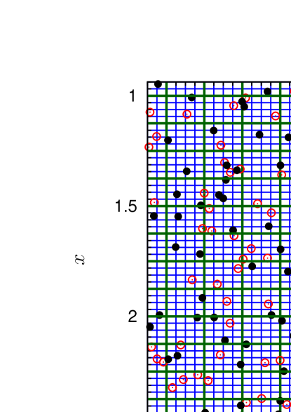
Figure 1: (Color online). The structure of the fine (blue solid lines) and coarse grids (green solid lines) are illustrated on a particular portion of the computational domain, together with positive and negative vortices indicated with empty red and filled black circles, respectively.

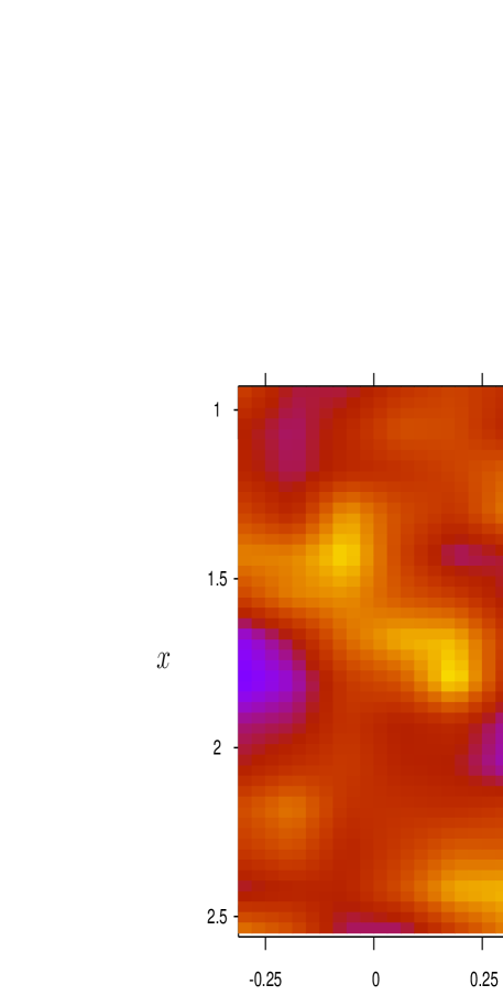
Figure 2: (Color online). Two–dimensional color plot of the longitudinal component of the mutual friction force $\widetilde{F}^{x}/\rho_{n}$ (see Eq. (16)), interpolated on the fine grid on the same domain as Fig. 1. The axes of the plot are rescaled employing the scaling units defined in Section III.1.

III Numerical simulations

III.1 Parameters

We chose the parameters of the numerical simulations in order to be able to make at least qualitative comparisons with experiments. As a reference, we select the experimental counterflow studies performed by Tough and collaborators on both high aspect–ratio rectangular cross–section channels, Ladner and Tough (1979) which represent the closest real experimental settings to our idealized plane channel, and cylindrical capillary tubes Childers and Tough (1976); Martin and Tough (1983). More in detail, we set the width of the channel $D=9.1\times 10^{-3}\,\rm cm$, corresponding to tube R4 in Ref. [Ladner and Tough, 1979], and $n^{1/2}D=25$. The consequent Reynolds number of the normal fluid flow calculated via Eq. (1) is $Re=206$, far below the critical Reynolds number for the onset of classical turbulent channel flows $Re_{c}\approx 5772$. Orszag (1971) As a consequence, on the basis also of past experimental investigations, Childers and Tough (1976); Ladner and Tough (1979); Martin and Tough (1983) we reckon that in our numerical experiment the flow of the normal fluid is still laminar.

$\,\,\,\,\,D\,\,\,\,\,$	$2$	$V_{n0}$	$553.6$
$L_{x}$	$6$	$T$	$1.7K$
$N$	$1876$	$\rho_{s}/\rho_{n}$	$3.373$
$n$	$\,\,\,\,\,\,\,156.3\,\,\,\,\,\,\,$	$\epsilon_{1}$	$2.5\times 10^{-3}$
$\ell$	$0.08$	$\Delta t_{v}$	$\,\,7.5\times 10^{-6}\,\,$

Table 1: Numerical parameters employed in the simulations
and subsequent physical relevant quantities in dimensionless units

The complete list of parameters employed in our simulation and the subsequent physical relevant quantities are reported in Table 1, expressed in terms of the following units of length, velocity and time, respectively: $\delta_{c}=D/2=4.55\times 10^{-3}\,\rm cm$, $u_{c}=\kappa/(2\pi\delta_{c})=3.49\times 10^{-2}\,\rm cm/s$, $t_{c}=\delta_{c}/u_{c}=0.13\,\rm s$. Hereafter all the quantities which we mention are dimensionless, unless otherwise stated. The constant $V_{n0}$ determining $u_{n}^{p}$ is computed imposing, without any loss of generality, that the whole normal fluid flow rate is supplied by the Poiseuille field $\mathbf{v}_{n}^{p}$, i.e. $\langle u_{n}\rangle=\langle u_{n}^{p}\rangle$, implying $\langle u_{n}^{\prime}\rangle=0$. In the spirit of the coarse–grained description illustrated in Section II.4, we define a coarse and a fine grid characterized by numbers of grid–points and spacings listed in Table 2, satisfying the condition $\Delta X,\Delta Y>\ell>\Delta x,\Delta y$.

Fine grid		Coarse grid
$\,\,n_{x}\,\,$	$192$	$\,\,N_{x}\,\,$	$48$
$n_{y}$	$64$	$N_{y}$	$16$
$\Delta x$	$\,\,3.125\times 10^{-2}\,\,$	$\Delta X$	$0.125$
$\Delta y$	$\,\,3.125\times 10^{-2}\,\,$	$\Delta Y$	$\,\,0.125\,\,$

Table 2: Number of grid–points and spacings in dimensionless units
of the grids employed in the numerical simulations

The coupled calculation of vortex motions and $\mathbf{v}_{n}$ entails the simultaneous existence of two different timestep stability criteria, one for each motion. Concerning the evolution equation (16) for $\omega_{n}^{\prime}$, the constraint is set by the normal fluid viscosity,Peyret and Taylor (1983) leading to the restriction $\Delta t_{n}\leq(\Delta x)^{2}/\nu$. Regarding the motion of the superfluid vortices, consistently with the numerical reconnection procedure illustrated in Section II.2, the integration timestep $\Delta t_{v}$ for Eq. (4) must satisfy the condition $\Delta t_{v}\leq\epsilon_{1}/(2V_{\epsilon_{1}})$, where $V_{\epsilon_{1}}$ is the velocity of a pair of anti–vortices along their separation vector when separated by a distance equal to $\epsilon_{1}$. This constraint on $\Delta t_{v}$ prevents from the generation of unphysical small–scale periodic motions (e.g. vortex–pairs multiple crossings). The value of $\Delta t_{v}$ employed in our simulation is reported in Table 1 and the viscous constraint allows us to set $\Delta t_{n}=2\Delta t_{v}$, implying that vortex motions alternately take place with frozen normal fluid.

III.2 Results

III.2.1 Steady–state regime

The aim of our numerical simulations is to determine the spatial distributions of positive and negative vortices and the normal fluid and superfluid velocity profiles across the channel in the steady–state regime. To stress that these distributions and profiles are meant to be coarse–grained over channel stripes of size $\Delta Y$, we use the $\overline{\,\cdot\,}$ symbols. Fig. 3 illustrates the initial conditions of a typical simulation. Fig. 3 (top) shows the initial random spatial distribution of the vortices, corresponding to the coarse–grained vortex density profiles $\overline{n}(y)$ shown in Fig. 3 (middle). In Fig. 3 (bottom) the initial parabolic Poiseuille profile for $\displaystyle\overline{u}_{n}$ and the flat profile for $\displaystyle\overline{u}_{s}$ are reported. After a transient interval whose characteristics will be addressed in section III.2.2, the system reaches the statistically–steady–state described in Fig. 4. As expected, the steady–state regime is achieved after a time interval $T_{f}\approx D^{2}/\nu$. The most important feature is the shape of the coarse–grained profile of the normal fluid velocity $\displaystyle\overline{u}_{n}$ reported in Fig. 4 (bottom), which is slightly flattened in the near–wall region and sharpened in the central region with respect to the Poiseuille profile. These characteristics have recently been observed experimentally by means of laser–induced fluorescence Marakov et al. (2015) in the same counterflow regime (turbulent superfluid, laminar normal fluid). In the experiment, the flattening of the profile is more pronounced, but we reckon that this difference is due, at least partially, to a larger superfluid turbulent intensity in the experimental setting ($40\lesssim L^{1/2}D\lesssim 70$ against $L^{1/2}D\simeq 25$ in our simulation).

The other key feature which emerges from the numerical simulation is the polarization of the superfluid vortex distribution, which can be qualitatively observed in the snapshot of the steady–state vortex configuration, Fig. 4 (top). To investigate quantitatively this aspect, we introduce the coarse–grained polarization vector $\overline{\mathbf{p}}(y)$ defined by Jou et al. (2008)

$$\overline{\mathbf{p}}(y)=\frac{\overline{\bm{\omega}}_{s}(y)}{\kappa\overline{n}(y)}=\frac{\overline{n}^{+}(y)-\overline{n}^{-}(y)}{\overline{n}^{+}(y)+\overline{n}^{-}(y)}\hat{\mathbf{z}}\,.$$ (22)

Note that $\overline{\mathbf{p}}(y)=\mathbf{0}$ when quantum turbulence is uniformly distributed all over the channel (as, for instance, at $t=0$ in our numerical simulations, see Fig. 3 (top) and (middle) ). The steady–state profile of the polarization magnitude $\overline{p}(y)$ is reported in Fig. 4 (middle) together with the positive and negative vortex density profiles, $\overline{n}^{+}(y)$ and $\overline{n}^{-}(y)$ respectively. This polarized pattern directly arises from the vortex–points equations of motion (4), where the friction term containing $\alpha$ depends on the polarity of vortex.

This polarization of the vortex configuration, which, we stress, is not complete, i.e. $|\overline{p}(y)|<1$, generates a parabolic coarse–grained superfluid velocity profile $\overline{u}_{s}(y)\sim y^{2}$ which is reported in Fig. 4 (bottom). This process, i.e. the superfluid polarization induced by a normal fluid shear generating a superfluid velocity pattern which mimics the normal fluid one, confirms past analytical results obtained via simple models Barenghi et al. (2002) and backs numerically observed normal fluid–superfluid velocity matching and vorticity locking. Samuels (1993); Barenghi et al. (1997, 2002); Morris et al. (2008)

It is interesting to notice that our model, although being two–dimensional, recovers the total vortex density profile $\overline{n}(y)$ computed very recently via three–dimensional numerical simulations of helium II channel counterflows with prescribed Poiseuille normal flow.Baggaley and Laizet (2013); Khomenko et al. (2015); Baggaley and Laurie (2015) On the contrary, the vortex density profile $\overline{n}(y)$ calculated in this work is significantly different from the ones computed in past two–dimensional simulations with prescribed Poiseuille normal flow, where the density is approximately uniform across the channel. Galantucci et al. (2011); Galantucci and Sciacca (2012)

III.2.2 Transient interval

The main results of our investigations have been outlined in the previous section. Before we finish, it is instructive to describe how the vortices and the normal fluid adjust to each other reaching a steady–state, starting from our arbitrary initial condition: this exercise helps to understand the physics of the coupling of vortices and normal fluid.

The evolution to the steady–state can be understood using the coarse–grained profile of the longitudinal component of the mutual friction force $\overline{F}^{x}$, reported in Fig. 6. The expression of $\overline{F}^{x}$ at a first order of accuracy according to Eq. (19), is

$$\overline{F}^{x}(y)\simeq-\alpha\rho_{s}\kappa\overline{n}(y)\left(\overline{u}_{n}(y)-\overline{u}_{s}(y)\right)$$ (23)

At $t=0$, $\overline{F}^{x}$ is stronger in the central region of the channel, flattening the profile of the normal fluid at time $t_{1}\simeq 6.8\times 10^{-3}T_{f}$ very close to the initial configuration, as illustrated in Fig. 5 (bottom). At times $t\simeq t_{1}$, the superfluid polarization is only partial, see Fig. 5 (top), generating a less pronounced superfluid velocity profile $\overline{u}_{s}(y)$ (Fig. 5 (bottom)). The resulting longitudinal component of the mutual friction force at $t\simeq t_{1}$ is therefore more uniform across the channel with respect to $t=0$, as illustrated in Fig. 6. This allows the normal fluid to regain a quasi parabolic profile in the subsequent time interval ($\overline{u}_{n}$ is approximately parabolic at $t\simeq 0.25T_{f}$). Finally, at $t=T_{f}$, the flow reaches a self–consistent dynamical equilibrium determined by (a) the vortex–density and velocity profiles reported in Fig. 4 (middle) and (bottom) and (b) the longitudinal component of the mutual friction force illustrated in Fig. 6, characterized by peak values in the near–wall region.

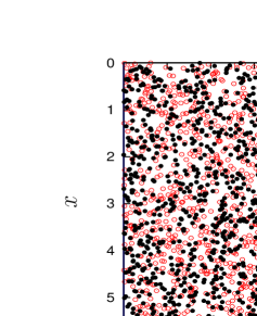
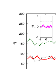
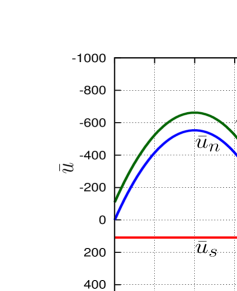
Figure 3: (Color online). (top): vortex distribution at $t=0$, red empty (black filled) circels indicate positive (negative) vortices; (middle): coarse–grained profiles of positive vortex density $\overline{n}^{+}$ (solid red line), negative vortex density $\overline{n}^{-}$ (dashed black line) and total vortex density $\overline{n}$ (dot–dashed green line) at $t=0$. In the inset, the corresponding coarse–grained profile of the polarization magnitude $\overline{p}(y)$ is reported (solid magenta line); (bottom) coarse–grained profiles of superfluid velocity $\overline{u}_{s}$ (solid red line), normal fluid velocity $\overline{u}_{n}$ (solid blue line) and counterflow velocity $\overline{u}_{ns}=\overline{u}_{n}-\overline{u}_{s}$ (solid green line) at $t=0$

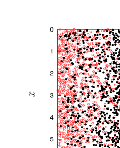
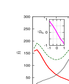
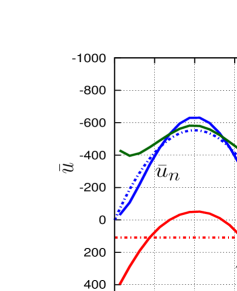
Figure 4: (Color online). (top): vortex distribution at $t=T_{f}$, red empty (black filled) circels indicate positive (negative) vortices; (middle): coarse–grained profiles of positive vortex density $\overline{n}^{+}$ (solid red line), negative vortex density $\overline{n}^{-}$ (dashed black line) and total vortex density $\overline{n}$ (dot–dashed green line) at $t=T_{f}$. In the inset, the corresponding coarse–grained profile of the polarization magnitude $\overline{p}(y)$ is reported (solid magenta line); (bottom) coarse–grained profiles of superfluid velocity $\overline{u}_{s}$ (solid red line), normal fluid velocity $\overline{u}_{n}$ (solid blue line) and counterflow velocity $\overline{u}_{ns}=\overline{u}_{n}-\overline{u}_{s}$ (solid green line) at $t=T_{f}$. Red and blue dot–dashed lines indicate the initial laminar profiles of the superfluid and the normal fluid, respectively.

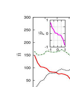
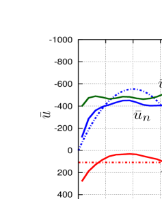
Figure 5: (Color online). (top): coarse–grained profiles of positive vortex density $\overline{n}^{+}$ (solid red line), negative vortex density $\overline{n}^{-}$ (dashed black line) and total vortex density $\overline{n}$ (dot–dashed green line) at $t=6.8\times 10^{-3}T_{f}$. In the inset, the corresponding coarse–grained profile of the polarization magnitude $\overline{p}(y)$ is reported (solid magenta line); (bottom) coarse–grained profiles of superfluid velocity $\overline{u}_{s}$ (solid red line), normal fluid velocity $\overline{u}_{n}$ (solid blue line) and counterflow velocity $\overline{u}_{ns}=\overline{u}_{n}-\overline{u}_{s}$ (solid green line) at $t=6.8\times 10^{-3}T_{f}$. Red and blue dot–dashed lines indicate the initial laminar profiles of the superfluid and the normal fluid, respectively.

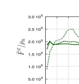
Figure 6: (Color online). Coarse–grained profile of the longitudinal component of the mutual friction force $\overline{F}^{x}$ at different selected times: $t=0$ (dot–dashed green line); $t=6.8\times 10^{-3}T_{f}$ (dashed green line); $t=T_{f}$ (solid green line).

IV Discussion

The aim of the present section is to (a) describe the idealized three–dimensional dynamics which we reckon corresponds to the two–dimensional vortex–points motion illustrated in Section III.2 and (b) critically discuss to what extent this idealized three–dimensional motion is capable of grasping the most relevant vortex–tangle dynamics occurring in helium II T-I counterflows. These two issues will be addressed in Sections IV.1 and IV.2, respectively.

IV.1 Streamwise flow of expanding vortex–rings

The two–dimensional vortex–points motion described in Section III.2, can be physically interpreted in three dimensions as an idealized streamwise flow of expanding vortex–rings lying on planes perpendicular to $\mathbf{v}_{n}^{p}$ and drifting in opposite direction with respect to $\mathbf{v}_{n}^{p}$. This vortex–ring three–dimensional analogue of the vortex–points motion stems from the vortex points equations of motion (4) and can be clearly discerned if we consider the motion of an anti–vortex pair whose initial configuration is symmetrical with respect to the mid plane of the channel and very close to the latter, see Fig. 7.

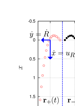
Figure 7: (Color online). Trajectories $\mathbf{r}_{+}(t)$ and $\mathbf{r}_{-}(t)$ of an anti–vortex pair, whose initial configuration is symmetric with respect to the mid plane of the channel (in dashed blue line). The time interval between consecutives positions is constant, indicating an increasing streamwise velocity as the vortex–points approach the walls. In an axisymmetric interpretation, the three–dimensional analogue of this two–dimensional motion is a streamwise flow of an expanding vortex ring.

Let $\mathbf{r}_{\pm}(t)=\left(x_{\pm}(t),y_{\pm}(t)\right)$ be the trajectories of the positive and negative vortices which consititute the anti–vortex pair, with initial condition $\left(x^{0}_{\pm},y^{0}_{\pm}\right)$. The axisymmetric hypothesis imposes $\left|y^{0}_{-}\right|=\left|y^{0}_{+}\right|=y^{0}$, while the proximity to the channel’s mid plane implies $y_{0}\ll 1$. According to the proposed parallel, the dynamics of this anti–vortex pair corresponds to the three–dimensional motion of a very small circular vortex ring centered on the channel’s mid plane and initial radius $R^{0}=y^{0}$. To obtain the typical motion of the pair of anti–vortices (corresponding to the intersections of the vortex ring with the two–dimensional channel), we average the vortex–points equation of motion (4) in the streamwise direction and over time deducing the following equation for $\displaystyle\overline{\frac{d\mathbf{r}_{\pm}}{dt}}$

$$\displaystyle\overline{\frac{d\mathbf{r}_{\pm}}{dt}}=\overline{\dot{\mathbf{r}}}_{\pm}=\left(\begin{array}[]{c}\overline{\dot{x}}_{\pm}(y)\\[5.69054pt] \overline{\dot{y}}_{\pm}(y)\end{array}\right)=\left(\begin{array}[]{c}(1-\alpha^{\prime})\overline{u}_{s}(y)+\alpha^{\prime}\overline{u}_{n}(y)\\[5.69054pt] \pm\alpha\left(\overline{u}_{n}(y)-\overline{u}_{s}(y)\right)\end{array}\right)\simeq\left(\begin{array}[]{c}\overline{u}_{s}(y)\\[5.69054pt] \pm\alpha\overline{u}_{ns}(y)\end{array}\right)$$ (30)

where the dot operator indicates the time derivative and $\overline{u}_{ns}=\overline{u}_{n}-\overline{u}_{s}$, to ease notation. In this simple axisymmetric anti–vortex pair model, $\overline{\dot{x}}_{\pm}=u_{R}$ and $\overline{\dot{y}}_{\pm}=\dot{R}$, where $u_{R}$ and $\dot{R}$ are the averaged vortex–ring streamwise drifting velocity and its expansion rate, respectively. We therefore have the following relations:

$$u_{R}(y)=(1-\alpha^{\prime})\overline{u}_{s}(y)+\alpha^{\prime}\overline{u}_{n}(y)$$ (31)

$$\dot{R}(y)=\pm\alpha\overline{u}_{ns}(y)$$ (32)

From equation 32, given the plot of $\overline{u}_{ns}(y)$ reported in Fig. 4, i.e. $\overline{u}_{ns}(y)<0\,\,\forall y$, it clearly emerges that the positive (negative) vortex moves towards the $y=-1$ ($y=1$). Hence, only the three-dimensional corresponding vortex rings whose circulation is oriented in the same direction of $\mathbf{v}_{n}^{p}$ expand, while vortex–rings of opposite circulation always shrink. The trajectory of an expanding anti–vortex pair is reported in Fig. 7.

We would like to stress, however, that our numerical simulations grasp a more general and complex dynamics, not enforcing an axisymmetric vortex–points motion, but moving each vortex individually. Therefore, the idealized three–dimensional vortex–ring motion described in the present paragraph is a physical interpretation of the average vortex–points motion only. We reckon, nevertheless, that it describes three–dimensionally the most relevant characteristics of the two–dimensional flow analyzed in the present model. In Fig. 8 several three–dimensional physical interpretations of the vortex–points motion are illustrated, with Fig. 8 (c) describing the vortex ring analog of the comprehensive two–dimensional motion described in Section III.2.

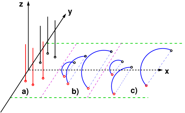
Figure 8: (Color online). Distinct three–dimensional interpretations of vortex–points motion: (a) straight vortices model; (b) idealized axisymmetric vortex ring interpretation described in Section IV.1; (c) vortex ring analog of the comprehensive two–dimensional motion.

IV.2 Congruity with vortex–tangle dynamics

Helium II counterflows are well known to exhibit anisotropic characteristics: the vortex lines tend to lie on planes perpendicular to $\mathbf{v}_{n}^{p}$. This can be easily deduced, for instance, by the plot of the projection of the vortex–line length in the streamwise direction $\langle\Lambda_{x}\rangle$ in Baggaley and Laurie (2015) and the plots of the anisotropic parameter $I^{\prime}$ in Yui and Tsubota (2015). As a consequence, we reckon that our idelized vortex–rings–flow model is able to capture the dynamics of the most relevant fraction of the vortex–tangle. In addition, it is worth emphasizing that the vortex–lines aligned in the streamwise direction (which we neglect in our simplified three–dimensional interpretation) are only affected very slightly by the mutual friction interaction which governs the vortex–tangle dynamics. On the other hand, our model is less reliable in the near–wall region where the vortex–tangle assumes a more isotropic character.

Furthermore, from Eqs. (31) and (32) and the plots of $u_{s}$, $u_{n}$ and $u_{ns}$ reported in Fig. 4 it is possible to deduce that in the proposed three–dimensional physical interpretation of our two–dimensional model, the vortex–rings drifting velocity in the streamwise direction increases as the radius of the vortex–rings grows (i.e. as the vortex–rings approach the channel walls). This vortex dynamics also emerges from past numerical three–dimensional studies Baggaley and Laurie (2015); Yui and Tsubota (2015) which describe the vortex lines moving towards the solid boundaries with increasing streamwise velocity in opposite direction with respect to the normal fluid flow.

To conclude this section, it is important to underline that the orientation of the expanding vortex–rings (circulation in the same direction of the normal fluid mean flow) is responsible for the non–uniform profile of $u_{s}$ illustrated in Fig. 4: the superfluid velocity field induced by such vortex–rings slows down the superflow in the central region of the channel while the image vortices increase the superfluid velocity near the boundaries. This non–uniform superfluid velocity profile is qualitatively recovered in past numerical simulations Yui and Tsubota (2015).

Having described what we propose is the three–dimensional physical interpretation of the vortex–points motion numerically investigated in our simulations and having discussed its consistency with the vortex–tangle dynamics observed in past three–dimensional numerical studies, we reckon that our model, although being two–dimensional, is capable of grasping the most essential and relevant dynamics taking place in helium II T-I channel counterflows.

V Conclusions

In this work we have performed two–dimensional self–consistent, coupled numerical simulations of helium II channel counterflows with corresponding vortex–line density typical of counterflow experiments.Ladner and Tough (1979); Martin and Tough (1983)

The main features of our model are the presence of solid boundaries and the dynamical coupling of vortices and normal fluid. These features make our model more realistic than previous investigations, although, due to computational constraints we had to use a two–dimensional geometry rather than a three–dimensional one. We reckon, however, that our model, despite its reduced dimensionality, is capable of grasping, at least qualitatively, the most relevant features of the vortex–tangle dynamics occurring in helium II T-I counterflows. For instance, the proposed physical three–dimensional interpretation of the vortex–points motion (i.e. a streamwise flow of expanding vortex rings) is qualitatively in agreement with the three–dimensional vortex–lines motion computed under prescribed normal fluid flow.Baggaley and Laurie (2015); Yui and Tsubota (2015) In addition, the vortex density profiles computed three–dimensionally with imposed Poiseuille normal fluid flow Baggaley and Laizet (2013); Khomenko et al. (2015); Baggaley and Laurie (2015) are consistent with the profiles calculated in our two–dimensional simulations. Experimentally, these profiles could be estimated by suitable second sound attentuation measurements, employing high harmonics waves.

In conclusion, the numerical results achieved in our work confirm the already observed velocity matching Barenghi et al. (2002) and vorticity locking Samuels (1993); Barenghi et al. (1997, 2002); Morris et al. (2008) between the two helium II components. Above all, our numerical model predicts the shape of the profile of the normal fluid which has been just observed experimentally in channels using laser–induced fluorescence of metastable helium molecules.Marakov et al. (2015) Furthermore, our results are useful for the interpretation of actual and future experiments, including pure superflow Babuin et al. (2012) and the motion of tracer particles.Chagovets and Van Sciver (2011); La Mantia et al. (2013)