Abstract

Dynamic buckling behavior of a column (rod, beam) under constant rate compression is considered. The buckling is caused by prescribed motion of column ends toward each other with constant velocity. Simple model with one degree of freedom simulating static and dynamic buckling of a column is derived. In the case of small initial disturbances the model yields simple analytical dependencies between the main parameters of the problem: critical force, compression rate, and initial disturbance. It is shown that the time required for buckling is inversely proportional to cubic root of compression velocity and logarithmically depends on the initial disturbance. Analytical expression for critical buckling force as a function of compression velocity is derived. It is shown that in a range of compression rates typical for laboratory experiments the dependence is accurately approximated by a power law with exponent close to $2/3$. Theoretical findings are supported by available results of laboratory experiments.

Keywords: dynamic buckling, Hoff problem, column, Airy equation, Euler force.

1 Introduction

Buckling of columns (rods, beams) under compression is a classical problem for mechanics of solids. In 1744 Leonard Euler predicted critical buckling force for compressed column in statics. Numerous experimental and theoretical studies have revealed that behavior of a column in dynamics is significantly more complicated. In particular, in dynamics the maximum force acting in the column, further refereed to as critical force, exceeds Euler force. Dynamic buckling behavior significantly depends on the way of compression. A review of different loading conditions may be found, for example, in a review paper [1]. Sudden application of a force was investigated, for example, in recent works [2, 3]. Mass falling on the rod was studied theoretically and experimentally in papers [4, 5]. In laboratory experiments the load-bearing capacity of columns is usually measured in hydraulic testing machines. In this case column ends move toward each other with prescribed velocity [6, 7]. This loading regime is also typical for computer simulation of buckling at macro [8] as well as micro and nano scale levels [9]. In 1951 Hoff has proposed the following simplified statement of this problem [6]. Compression of a column with initial imperfection in a form of a sine wave was considered. It was assumed that the deflection of a column has the shape of the first buckling mode. This assumption yields the nonlinear differential equation describing buckling of a column. In particular, Hoff has shown that the critical force strongly depends on compression rate and initial imperfection of a column. Buckling under constant rate compression in Hoff’s statement was studied in papers [8, 11, 12, 13, 14]. The influence of axial inertia [11], random imperfection [13] and boundary conditions [8] was investigated. Approximate solutions of Hoff’s equation are discussed in papers [12, 14]. The dependence of critical buckling force on the rate of compression is obtained by fitting the numerical numerical results [8]. Recent experiments [7] has revealed that the dependence is accurately approximated by the power law. However to our knowledge theoretical explanation of this fact is not present in the literature.

In the present paper simple one-dimensional model of dynamic buckling under constant rate compression is presented. It is assumed that the equilibrium configuration of the column is perfectly straight. Understanding of buckling of perfect columns is especially important at nano scale [9, 10], because nano-objects may have no defects. The disturbance is introduced by non-zero initial deflection. At nano scale it might be associated with thermal motion. Analytical dependencies of the time required for buckling and critical force on compression rate are derived. Theoretical findings are supported by the results of laboratory experiments [7].

2 One-dimensional model, analytical solution

Consider simple structural model reflecting the main physical features of a column subjected to constant rate compression. The column is simulated by a particle (point mass) connected with two walls by linear springs with stiffness $c_{L}$ and equilibrium length $a_{0}$ (see figure 1).

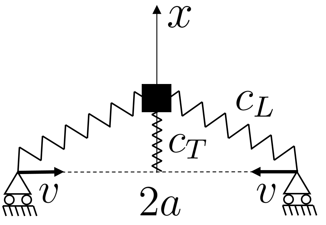
Figure 1: Structural model for dynamic buckling of a column under constant rate compression.

Transverse stiffness of the column is simulated by a spring with stiffness $c_{T}$ connecting the particle with middle point between the walls (see figure 1). The walls move toward each other with constant velocity $v$. Potential energy of the system has the form:

$$U=c_{L}(\sqrt{a^{2}+x^{2}}-a_{0})^{2}+\frac{1}{2}c_{T}x^{2},$$ (1)

where $x$ is a coordinate of the particle; $a,a_{0}$ are the current and initial half distances between the walls.

For any distance between the walls $2a$ the straight configuration of the system $x=0$ is an equilibrium. At some distance between the walls this equilibrium becomes unstable and two additional stable equilibria exist:

$$x_{1,2}=\pm\sqrt{a_{E}^{2}-a^{2}},\quad a\leq a_{E},\qquad a_{E}=\frac{2c_{l}a_{0}}{2c_{L}+c_{T}}.$$ (2)

Here $a_{E}$ is a bifurcation point corresponding to critical half-distance between the walls. It can be show that for $a>a_{E}$ the straight configuration on the system ($x=0$) is unstable. Stable equilibria are defined by formula (2). Corresponding Euler-like critical force in statics is

$$F_{E}=c_{L}a_{0}\varepsilon_{E},\qquad\varepsilon_{E}=1-\frac{a_{E}}{a_{0}}=\frac{c_{T}}{2c_{L}+c_{T}},$$ (3)

where $\varepsilon_{E}$ is a critical deformation in statics. Thus static behavior of the system is qualitatively similar to the behavior of the column under compression. Below critical deformation the straight configuration of the system is stable. For higher deformations there are two symmetric equilibria (2). Critical value of the force corresponding to static buckling is given by formula (3).

Consider the influence of dynamic effects on critical buckling force. Only transverse motions of the particle are considered. The effect of axial inertia is small and can be neglected [11]. The equation of transverse motion of the particle is

$$m\ddot{x}=-\left(2c_{L}+c_{T}-\frac{2c_{L}a_{0}}{\sqrt{a^{2}+x^{2}}}\right)x,\quad x(-t_{E})=x_{0},\quad\dot{x}(-t_{E})=0,\qquad a=a_{E}-vt.$$ (4)

where $m$ is mass of the particle, $x_{0}$ is an initial deflection. Loading is applied at $t=-t_{E}$, where $t_{E}=(a_{0}-a_{E})/v$ is a time required for reaching Euler static force. Initial disturbance is simulated by non-zero initial deflection $x_{0}$. Note that the statement used by Hoff is different [6]. In paper [6] it is assumed that natural configuration of the column has finite curvature. In the present paper perfectly straight column is considered.

Horizontal component of the force (see fig. 1) acting on the walls has the form:

$$F=c_{L}(a_{E}-vt)\left(\frac{a_{0}}{\sqrt{(a_{E}-vt)^{2}+x^{2}}}-1\right).$$ (5)

The force $F$ has maximum value at moment of time $t_{*}$, further refereed to as time required for buckling [4]. Parameter $t_{*}$ is defined by the equation:

$$\frac{{\rm d}}{{\rm d}t}F(x(t,v,x_{0}),vt)|_{t=t_{*}}=0\quad\Rightarrow\quad t_{*}=t_{*}(v,x_{0}).$$ (6)

Equation (6) yields the dependence of $t_{*}$ on $v$ in the implicit form. Substituting $x(t_{*})$ and $t_{*}(v,x_{0})$ into equation (5) yields the expression for the critical buckling force:

$$F_{*}=c_{L}(a_{E}-vt_{*})\left(\frac{a_{0}}{\sqrt{(a_{E}-vt_{*})^{2}+x_{*}^{2}}}-1\right),\qquad x_{*}=x(t_{*},v,x_{0}).$$ (7)

The dependencies $t_{*}(v,x_{0})$, $x(t_{*},v,x_{0})$ are given in the implicit form by nonlinear equations (4), (6).

The exact solution of equations (4), (6) in the general case is not straightforward. Therefore the following assumptions are used

$$vt_{*}\ll a_{E},\quad|x_{*}|\ll a_{E}.$$ (8)

Linearize the expression for critical force with respect to small parameters $x_{*}$ and $vt_{*}$:

$$F_{*}\approx F_{E}+c_{L}vt_{*}-c_{L}\frac{a_{0}x_{*}^{2}}{2a_{E}^{2}}.$$ (9)

The relation between $t_{*}$ and $v$ is derived as follows. The force $F$ is expanded into series with respect to $vt$ and $x$ and then substituted into (6):

$$\frac{{\rm d}F}{{\rm d}t}|_{t=t_{*}}\approx c_{L}\left(v-\frac{a_{0}}{a_{E}^{2}}x_{*}\dot{x}_{*}\right)=0.$$ (10)

Critical values of displacement $x(t_{*})$ and velocity $\dot{x}(t_{*})$ are calculated using the equation of motion (4). The latter is linearized under assumptions (8):

$$\ddot{x}-\alpha vtx=0,\qquad\alpha=\frac{2c_{L}a_{0}}{ma_{E}^{2}}.$$ (11)

The equation (11) is usually referred to as Airy’s equation (see e.g. [15]). The solution of equation (11) is a linear combination of Airy’s functions ${\rm Ai}$ and ${\rm Bi}$ [15]:

$$\begin{array}[]{l}\displaystyle x(t)=C_{1}{\rm Ai}\left(t\alpha^{\frac{1}{3}}v^{\frac{1}{3}}\right)+C_{2}{\rm Bi}\left(t\alpha^{\frac{1}{3}}v^{\frac{1}{3}}\right),\qquad\tau_{E}=\alpha^{\frac{1}{3}}(a_{E}-a_{0})v^{-\frac{2}{3}},\\[11.38109pt] \displaystyle C_{1}=\frac{x_{0}{\rm Bi^{\prime}}(\tau_{E})}{{\rm Bi^{\prime}}(\tau_{E}){\rm Ai}(\tau_{E})-{\rm Bi}(\tau_{E}){\rm Ai^{\prime}}(\tau_{E})},\quad C_{2}=-\frac{x_{0}{\rm Ai^{\prime}}(\tau_{E})}{{\rm Bi^{\prime}}(\tau_{E}){\rm Ai}(\tau_{E})-{\rm Bi}(\tau_{E}){\rm Ai^{\prime}}(\tau_{E})}.\end{array}$$ (12)

For positive arguments ${\rm Ai}$ exponentially decays and ${\rm Bi}$ exponentially grows [15]. In particular, for large values of the argument the following asymptotic formulas can be used:

$${\rm Ai}(z)\sim\frac{e^{-\frac{2}{3}z^{\frac{3}{2}}}}{2\sqrt{\pi}z^{\frac{1}{4}}},\quad{\rm Ai}^{\prime}(-z)\sim\frac{\cos\left(\frac{2}{3}z^{\frac{3}{2}}+\frac{\pi}{4}\right)z^{\frac{1}{4}}}{\sqrt{\pi}},\quad{\rm Bi}(z)\sim\frac{e^{\frac{2}{3}z^{\frac{3}{2}}}}{\sqrt{\pi}z^{\frac{1}{4}}}.$$ (13)

Therefore the first term in the expression (12) for $x(t)$ is neglected. Then asymptotic formulas (13) and formula (10) yields the following implicit relation between $t_{*}$ and $v$:

$$\left(\frac{v}{v_{s}}\right)^{\frac{2}{3}}=\frac{\pi^{2}{\rm Ai^{\prime}(\tau_{E})^{2}}}{(1-\varepsilon_{E})^{\frac{8}{3}}}\left(\frac{x_{0}}{a_{0}}\right)^{2}{\rm Bi}\left(\tau_{*}\right){\rm Bi}^{\prime}\left(\tau_{*}\right),\qquad\tau_{*}=t_{*}\alpha^{\frac{1}{3}}v^{\frac{1}{3}},$$ (14)

where $v_{s}=a_{0}\sqrt{2c_{L}/m}$ is a characteristic velocity, corresponding to velocity of longitudinal waves in the column. For small initial disturbances $x_{0}^{2}$ and finite compression rates $v$ parameter $\tau_{*}$, defined by formula (14), is large. Then using asymptotic formulas (13) in (14) yields the explicit dependence of the time required for buckling $t_{*}$ on the compression rate:

$$\frac{t_{*}}{t_{s}}=g(v)\left(\frac{v_{s}}{v}\right)^{\frac{1}{3}},\qquad g(v)=\left(\frac{1-\varepsilon_{E}}{2}\ln\frac{va_{0}^{3}(1-\varepsilon_{E})^{4}}{\pi^{\frac{3}{2}}v_{s}x_{0}^{3}{\rm Ai^{\prime}}(\tau_{E})^{3}}\right)^{\frac{2}{3}}.$$ (15)

where $t_{s}=a_{0}/v_{s}$. For small initial disturbances $x_{0}^{2}$ and finite velocities $v$ the dependence $g(v)$ is weak. Therefore the time required for buckling is inversely proportional to cubic root of the compression rate.

Consider the contribution of $vt_{*}$ and $x_{*}^{2}$ to the critical force (9). For large $\tau_{*}$ formula (14) yields:

$$\frac{vt_{*}a_{0}}{x_{*}^{2}}\sim\frac{\tau_{*}{\rm Bi}^{\prime}\left(\tau_{*}\right)}{{\rm Bi}\left(\tau_{*}\right)}\gg 1.$$ (16)

Then the last term in the formula (9) can be neglected.

Substitution of formula (15) into equation (9) yields the dependence of the critical force of the compression rate:

$$\frac{F_{*}}{F_{E}}=1+\frac{g(v)}{\varepsilon_{E}}\left(\frac{v}{v_{s}}\right)^{\frac{2}{3}}.$$ (17)

Estimate critical deformation $\varepsilon_{E}$ for a column. For Bernoulli-Euler beam with square cross-section, thickness $h$ and length $l$ the expression for $\varepsilon_{E}$ has the form:

$$\varepsilon_{E}=\frac{\pi^{2}}{12}\left(\frac{h}{l}\right)^{2}.$$ (18)

Formulas (17) and (18) yield the expression for critical force:

$$\frac{F_{*}}{F_{E}}=1+\frac{12g(v)}{\pi^{2}}\left(\frac{l}{h}\right)^{p}\left(\frac{v}{v_{s}}\right)^{q},\qquad p=2,\qquad q=\frac{2}{3}.$$ (19)

The dependence of $g$ on $v$ and $l/h$ is relatively weak. Therefore critical force and compression rate are related by the power law dependence. This result is in a good agreement with experimental data [5, 7]. In paper [7] compression of columns with constant rate in a hydraulic machine was investigated. In paper [5] buckling under the action a heavy body falling on the end of the column was considered. In both cases the dependence of critical force on the compression rate is approximated by formula, similar to (17). The following values of parameters $p,q$ were obtained: $p=2.0,q=0.68$ [5] and $p=1.61,q=0.62$ [7].

Estimate the interval of compression rates, where formula (17) is applicable. The derivation is based on the assumption $C_{2}\neq 0$. It is straightforward to show that $C_{2}=0$ at some points of the interval $\tau_{E}<-1$. Then compression rate should satisfy the following condition:

$$\frac{v}{v_{s}}>\frac{\varepsilon_{E}^{\frac{3}{2}}}{1-\varepsilon_{E}}.$$ (20)

Additionally, the assumption $\tau_{*}>1$ was used. Using this condition in formula (14) yields:

$$\frac{v}{v_{s}}>\frac{\pi^{3}{\rm Ai^{\prime}(\tau_{E})^{3}}}{(1-\varepsilon_{E})^{4}}\left(\frac{x_{0}}{a_{0}}\right)^{3}{\rm Bi}\left(1\right)^{\frac{3}{2}}{\rm Bi}^{\prime}\left(1\right)^{\frac{3}{2}}.$$ (21)

Thus formula (17) describes the behavior of the system at velocities and initial disturbances satisfying conditions (20) and (21).

3 Comparison with numerical solution

The model described above involves significant simplifications. In the present section the analytical results are compared with numerical solution of the exact nonlinear equation (4). The equation of motion (4) is solved numerically using Verlet symplectic integration scheme. Initial velocity is equal to zero, initial displacement is equal to $x_{0}$. The following values of dimensionless parameters are used $c_{T}/c_{L}=1.64\cdot 10^{-6}$, $\Delta t/t_{s}=10^{-2}$. The given ratio of stiffnesses corresponds to the column with length/thickness ratio about $10^{3}$ (see formula (18)). Velocity belongs to the interval $v/v_{s}\in[10^{-8};10^{-3}]$ considered in laboratory experiments [7].

In the simulations the longitudinal force is computed using formula (5). Typical dependence of the force on deformation for $x_{0}/a=10^{-4}$ and $v/v_{s}=10^{-10},10^{-9},10^{-8}$ is shown in figure 2. Critical force $F_{*}$ corresponds to the maximum value of the force shown in figure 2.

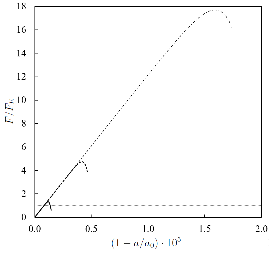
Figure 2: Dependence of longitudinal force on deformation for $x_{0}/a=10^{-4}$,  $v/v_{s}=10^{-8}$ (dash-dot line), $10^{-9}$ (dashed line), $10^{-10}$ (solid line). Horizontal line corresponds to the Euler static force.

Though the velocity is much lower then the “velocity of sound” $v_{s}$, the critical force significantly exceeds Euler static force (3).

The dependence of critical force on the rate of compression $v$ for initial disturbances $x_{0}/a_{0}=10^{-3},10^{-12}$ is shown in figure 3.

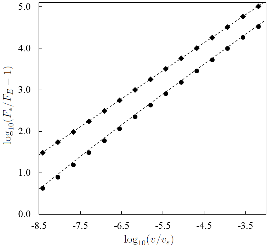
Figure 3: Dependence of critical buckling force on compression rate for initial disturbances $x_{0}/a_{0}=10^{-3}$ (circles), $10^{-12}$ (diamonds). Points correspond to numerical solution, lines correspond to analytical solution (formula (17)).

It is seen that the dependence is accurately approximated by the power law (17). The power tends to $2/3$ as the initial disturbance tends to zero.

4 Conclusions

Simple one-dimensional model for dynamic buckling of a column under constant rate compression is derived. Despite the simplicity, the model qualitatively the influence of the main parameters (compression rate, length/thicknessration, and initial disturbance) on the critical force. In dynamics the critical force buckling exceeds the Euler force even at relatively slow compression rates. The reason is that some time is required for transition from unstable straight configuration to stable bend configuration. It is shown that this time is inversely proportional to cubic root of velocity of column end. For small initial disturbances the dependence of critical force on velocity of the end is accurately approximated by the power law with exponent approximately equal to $2/3$. This result is in a good agreement with the results of laboratory experiments [5, 7].

References

- [1] D. Karagiozova, M. Alves, Dynamic elastic-plastic buckling of structural elements: A Review. Applied Mechanics Reviews, 2008, Vol. 61.
- [2] A.K. Belyaev, D.N. Il in, N.F. Morozov, Dynamic approach to the Ishlinsky Lavrent ev problem, Mech. Sol., 2013, Vol. 48, No. 5, pp. 504–508.
- [3] N.F. Morozov, P.E. Tovstik, T.P. Tovstik, Again on the Ishlinskii–Lavrentyev problem, Doklady Physics, 2014, Vol. 59, No. 4, pp. 189–192.
- [4] W. Ji, A.M. Waas, Dynamic bifurcation buckling of an impacted column. Int. J. Eng. Sci., 2008, Vol. 46, pp. 958 -967.
- [5] K. Mimura, T. Umeda, M. Yu, Y. Uchida, H. Yaka, Effects of impact velocity and slenderness ratio on dynamic buckling load for long columns. Int. J. Mod. Phys. B, Vol. 22, Nos. 31, 32, 2008, pp. 5596- 5602.
- [6] Hoff N.J. The dynamics of the buckling of elastic columns. J. Appl. Mech. 1951, Vol. 18, pp. 68 -74.
- [7] K. Mimura, T. Kikui, N. Nishide, T. Umeda, I. Riku, H. Hashimoto Buckling behavior of clamped and intermediately-suported long rods in the static-dynamic transition velocity region. J. Soc. Mat. Sci., Vol. 61, No. 11, pp. 881—887, 2012.
- [8] P. Motamarri, S. Suryanarayan, Unified analytical solution for dynamic elastic buckling of beams for various boundary conditions and loading rates. Int. J. Mech. Sci., 56, 2012, pp. 60- 69.
- [9] H. Shima, Buckling of Carbon Nanotubes: A State of the Art Review. Materials 2012, 5, pp. 47-84.
- [10] C.Y. Tang, L.C. Zhang, K. Mylvaganam. Rate dependent deformation of a silicon nanowire under uniaxial compression: Yielding, buckling and constitutive description. Comp. Mat. Sci. 51, 2012, pp. 117- 121.
- [11] E. Sevin On the elastic bending of columns due to dynamic axial forces including effects of axial inertia. J. Appl. Mech., 1960, 27(1), pp. 125-131.
- [12] Dym C.L., Rasmussen M.L. On a perturbation problem in structural dynamics, Int. J. of Non-Linear Mech., 3 (2), 1968, pp. 215-225
- [13] I. Elishakoff, Hoff’s Problem in a Probabilistic Setting. J. App. Mech., 1980, Vol. 47.
- [14] A. N. Kounadis, J. Mallis, Dynamic stability of initially crooked columns under a time-dependent axial displacement of their support. Q. J. Mech. Math., Vol. 41, 4, 1988.
- [15] F.W.J. Olver, D.W. Lozier, R.F. Boisvert, W. Clark, NIST Handbook of Mathematical Functions, Cambridge University Press, 2010.