Hadron-Hadron Interactions from $N_{f}=2+1+1$ Lattice QCD:
isospin-2 $\pi\pi$ scattering length

Abstract

We present results for the $I=2$ $\pi\pi$ scattering length using $N_{f}=2+1+1$ twisted mass lattice QCD for three values of the lattice spacing and a range of pion mass values. Due to the use of Laplacian Heaviside smearing our statistical errors are reduced compared to previous lattice studies. A detailed investigation of systematic effects such as discretisation effects, volume effects, and pollution of excited and thermal states is performed. After extrapolation to the physical point using chiral perturbation theory at NLO we obtain $M_{\pi}a_{0}=-0.0442(2)_{\mathrm{stat}}(^{+4}_{-0})_{\mathrm{sys}}$.

1 Introduction

Quantum Chromodynamics (QCD) describes, beyond the mass spectrum of stable and unstable hadrons, also their interaction due to the strong force. While originally thought to be not accessible to lattice QCD [1], Martin Lüscher was able to relate the energy spectrum in finite volume to the infinite volume interaction properties in a series of seminal papers [2, 3, 4, 5]. During the last years, extensions of these finite volume techniques have been worked out and they have been applied to a number of interesting systems.

Lüscher’s original formalism dealt with two massive bosons in a finite cubic box below the inelastic scattering threshold. It was originally formulated for the center of mass frame. In order to enlarge the applicability of Lüscher’s method, extensions have been developed over the years which include: moving frames with non-vanishing center of mass momentum [6, 7, 8, 9], asymmetric boxes [10, 11, 12], twisted boundary conditions [13, 14, 15, 16], and more. Most of these aim to circumvent the poor resolution in momentum space due to the quantisation of the three-momentum in finite volume. Generalisations beyond the inelastic threshold for the two particle cases are also discussed [17, 18, 19, 20, 21, 22] and various groups are now working on the more difficult three-particle scenario [23, 24, 25, 26, 27, 28, 29].

In this first paper of a planned series of papers we investigate $\pi\pi$ scattering in the isospin-2 channel. $\pi\pi$ scattering in the $I=2$ channel is technically the easiest case to consider in lattice QCD, because so-called fermionic disconnected contributions are absent. Moreover, the predicted quark mass dependence in chiral perturbation theory ($\chi$PT) at next-to-leading order (NLO) is governed by only one low energy constant, and so far lattice data showed surprisingly little deviations even from the leading order (LO) $\chi$PT predictions, which is parameter free. Isospin-2 $\pi\pi$ scattering is, therefore, an important benchmark system to compare with non-lattice methods and an important test case for future investigations of hadron-hadron interactions, while simultaneously of phenomenological interest.

Consequently, it has been computed in lattice QCD previously [30, 31, 32, 33, 34] using $N_{f}=2$ or $N_{f}=2+1$ dynamical fermions, for a recent review see Ref. [35]. In this paper we extend this list by using $N_{f}=2+1+1$ dynamical quark flavours for the first time. The analysis relies on Wilson twisted mass fermions [36] at maximal twist [37] based on gauge configurations provided by the European Twisted Mass Collaboration (ETMC) [38, 39]. This allows us to investigate a range of pion masses from $250$ to $500\ \mathrm{MeV}$ and discretisation effects by using three values of the lattice spacing. For estimating finite volume effects we have several ensembles at our disposal with all parameters fixed but the volume.

We apply different strategies to determine scattering parameters from the data using Lüscher’s finite volume method. This gives us an estimate of residual finite volume effects on the scattering length for other ensembles where we do not have multiple volumes at hand.

The main result is an extrapolation of $M_{\pi}a_{0}$ to the physical point utilising chiral perturbation theory at next-to-leading order. We carry systematic effects from different fit ranges through the entire analysis chain. In addition we investigate the stability of the extrapolation by different cuts in the pion mass values.

The paper is structured as follows: in section 2 we review the fermion action, the Laplacian-Heaviside smearing technique and the interpolating operators we use to construct the correlation functions. Lüscher’s finite volume method is explained in section 3. Our analysis and the treatment of all sources of systematic effects are worked out in section 4. The final results are discussed in section 5 and summarised in section 6.

2 Lattice action

ensemble	$\beta$	$a\mu_{\ell}$	$a\mu_{\sigma}$	$a\mu_{\delta}$	$(L/a)^{3}\times T/a$	$N_{\mathrm{conf}}$
$A30.32$	$1.90$	$0.0030$	$0.150$	$0.190$	$32^{3}\times 64$	$280$
$A40.20$	$1.90$	$0.0040$	$0.150$	$0.190$	$20^{3}\times 48$	$553$
$A40.24$	$1.90$	$0.0040$	$0.150$	$0.190$	$24^{3}\times 48$	$404$
$A40.32$	$1.90$	$0.0040$	$0.150$	$0.190$	$32^{3}\times 64$	$250$
$A60.24$	$1.90$	$0.0060$	$0.150$	$0.190$	$24^{3}\times 48$	$314$
$A80.24$	$1.90$	$0.0080$	$0.150$	$0.190$	$24^{3}\times 48$	$306$
$A100.24$	$1.90$	$0.0100$	$0.150$	$0.190$	$24^{3}\times 48$	$312$
$B35.32$	$1.95$	$0.0035$	$0.135$	$0.170$	$32^{3}\times 64$	$250$
$B55.32$	$1.95$	$0.0055$	$0.135$	$0.170$	$32^{3}\times 64$	$311$
$B85.24$	$1.95$	$0.0085$	$0.135$	$0.170$	$32^{3}\times 64$	$296$
$D45.32sc$	$2.10$	$0.0045$	$0.0937$	$0.1077$	$32^{3}\times 64$	$301$

Table 1: The gauge ensembles used in this study. For the labelling of the ensembles we adopted the notation in Ref. [38]. In addition to the relevant input parameters we give the lattice volume and the number of evaluated configurations, $N_{\mathrm{conf}}$.

The sea quarks are described by the Wilson twisted mass action with $N_{f}=2+1+1$ dynamical quark flavours. The Dirac operator for the light quark doublet reads [36]

$$D_{\ell}=D_{\mathrm{W}}+m_{0}+i\mu_{\ell}\gamma_{5}\tau^{3}\,,$$ (1)

where $D_{\mathrm{W}}$ denotes the standard Wilson Dirac operator and $\mu_{\ell}$ the bare light twisted mass parameter. $\tau^{3}$ and in general $\tau^{i},i=1,2,3$ represent the Pauli matrices acting in flavour space. $D_{\ell}$ acts on a spinor $\chi_{\ell}=(u,d)^{T}$ and, hence, the $u$ ($d$) quark has twisted mass $+\mu_{\ell}$ ($-\mu_{\ell}$).

For the heavy unitary doublet of $c$ and $s$ quarks [40] the Dirac operator is given by

$$D_{\mathrm{h}}=D_{\mathrm{W}}+m_{0}+i\mu_{\sigma}\gamma_{5}\tau^{1}+\mu_{\delta}\tau^{3}\,.$$ (2)

The bare Wilson quark mass $m_{0}$ has been tuned to its critical value [41, 38]. This guarantees automatic order $\mathcal{O}\left(a\right)$ improvement [37], which is one of the main advantages of the Wilson twisted mass formulation of lattice QCD.

The splitting term in the heavy doublet Eq. 2 introduces flavour mixing between strange and charm quarks which needs to be accounted for in the analysis. However, this is only important for quantities involving valence strange and charm quarks.

2.1 Stochastic Laplacian Heavyside Smearing

On the long term we plan to address as many observables as possible. Hence we have decided to use the stochastic Laplacian Heavyside smearing (sLapH), which is quite generally applicable and which is described in detail in Refs. [42, 43]. It represents a smearing method based on the covariant 3-dimensional Laplace operator

$$\widetilde{\Delta}^{ab}(x,y;U)=\sum_{k=1}^{3}\Bigl{\{}\widetilde{U}_{k}^{ab}(x)\delta(y,x+\hat{k})+\widetilde{U}^{ba}_{k}(y)^{\dagger}\delta(y,x-\hat{k})-2\delta(x,y)\delta^{ab}\Bigr{\}}\,,$$ (3)

where $a,b$ are colour indices, $x,y$ space-time coordinates, $\widetilde{U}$ denote smeared gauge links, and the sum is taken over the three spatial directions. The gauge fields in the Laplace operator, Eq. 3, are smeared with three steps of three dimensional HYP smearing [44] with smearing parameters $\alpha_{1}=\alpha_{2}=0.62$, independently of the volume and lattice spacing. The Laplace operator can be decomposed as follows

$$\widetilde{\Delta}=V_{\Delta}\Lambda_{\Delta}V_{\Delta}^{\dagger}\,,$$ (4)

where $V_{\Delta}$ represents the matrix of all eigenvectors and $\Lambda_{\Delta}$ is a diagonal matrix containing the eigenvalues. Colour, Dirac and space-time indices are suppressed. The smearing matrix then reads

$$\mathcal{S}=V_{\mathrm{s}}V_{\mathrm{s}}^{\dagger}\,,$$ (5)

where $V_{\mathrm{s}}$ only contains eigenvectors corresponding to eigenvalues smaller than a cut-off $\sigma_{s}^{2}$. These eigenvectors span what is called the LapH sub-space. The value $\sigma_{s}^{2}$ can be chosen in a way that excited state contaminations are maximally suppressed. In Ref. [43] it has been found that $\sigma_{s}^{2}=0.33$ is optimal for excited state suppression independent of the interpolating operator. On a $48^{3}\times 96$ lattice, for example, this amounts to about 960 eigenvectors per time slice. However, our tests show that it is better to have less eigenvectors for these large lattices, namely $660$ on $48^{3}\times 96$ and $220$ on $32^{3}\times 64$, to suppress excited state contaminations at early Euclidean times.

The building blocks of observables are quark lines, $\mathcal{Q}$, which can be written in the LapH framework as

$$\mathcal{Q}=\mathcal{S}\Omega^{-1}\mathcal{S}=V_{\mathrm{s}}\ (V_{\mathrm{s}}^{\dagger}\Omega^{-1}V_{\mathrm{s}})\ V_{\mathrm{s}}^{\dagger}\,,$$ (6)

where the middle part, $\mathcal{P}=V_{\mathrm{s}}^{\dagger}\Omega^{-1}V_{\mathrm{s}}$, is called perambulator with $\Omega=\gamma_{4}M$ and $M$ being the Dirac operator. To generate a perambulator it is necessary to invert the Dirac operator for every eigenvector in $V_{\mathrm{s}}$. It follows that for an all-to-all perambulator, since the Laplace operator is diagonal in time and Dirac space, this procedure needs to be repeated for each time slice and Dirac component. Taking the $48^{3}\times 96$ lattice as an example this would result in a total number of $253440$ inversions. This number can be reduced significantly by combining the LapH method with a stochastic approach as described in Ref. [43] in detail.

For constructing all-to-all propagators with a stochastic approach, random vectors $\rho$ are introduced which carry Dirac, time, colour and spatial indices. A propagator can be computed by solving

$$\Omega X^{r[b]}=\rho^{r[b]}$$ (7)

for $X^{r[b]}$. Here the random vectors are not chosen to be random valued in all elements, but diluted, which is used to reduce the stochastic noise, see Ref. [43] for details. Correspondingly, the composed index $r[b]$ counts the total number of random vectors, $N_{\mathrm{R}}$, via $r$ and the total number of dilution vectors, $N_{\mathrm{D}}$, via $b$. When constructing the all-to-all propagator via

$$\Omega^{-1}\approx\frac{1}{N_{\mathrm{R}}}\sum_{r=1}^{N_{\mathrm{R}}}\sum_{b}X^{r[b]}\rho^{r[b]\dagger}\,,$$ (8)

the zeros in the diluted random vectors ensure exact zeros in the product $\rho^{r[b]}\rho^{r[b]\dagger}$, which reduces noise significantly. However, diluting random vectors leads to higher computational costs due to solving Eq. 7 for each of these vectors separately. It is expected that the noise in correlation functions built from diluted stochastic propagators reduces with $\nicefrac{{1}}{{\sqrt{N_{\mathrm{R}}}}}$ and $\nicefrac{{1}}{{N_{\mathrm{D}}}}$, which favours more dilution vectors over more random vectors. Aside from this, each quark line needs its own set of random vectors to avoid a bias in the correlation functions.

In the stochastic version of LapH, denoted by sLapH, the random vectors are introduced in time, Dirac and Laph sub-space indices. A quark line can then be estimated stochastically via

$${\mathcal{Q}}\approx\frac{1}{N_{\mathrm{R}}}\sum_{r=1}^{N_{\mathrm{R}}}\sum_{b}{\mathcal{S}}\Omega^{-1}\ V_{\mathrm{s}}\rho^{r[b]}\ (V_{\mathrm{s}}\rho^{r[b]})^{\dagger}\,.$$ (9)

In our implementation we choose $Z_{2}$ random numbers. As mentioned before each quark line as defined in Eq. 9, needs its own random vector to avoid a bias. This means that at least four random vectors are needed to be able to compute the correlation functions relevant for $\pi\pi$ scattering processes. However, we use five random vectors, since the fifth random vector will allow for additional permutations in the four point functions. This improves the signal-to-noise ratio by a factor of 2 by only increasing the computing costs for inversions by $25\%$.

As dilution scheme we have chosen full dilution in Dirac space combined with a block dilution in time and an interlace dilution in the LapH sub-space. The number of dilution vectors are summarised in table 2. They were chosen in such a way that the number of inversions and the noise in our observables are minimised simultaneously.

We remark here that with the sLapH smearing scheme as explained above, only smeared-smeared correlation functions can be computed. Hence, we cannot compute matrix elements of local operators needed for instance for $f_{\pi}$ without major additional effort.

$(L/a)^{3}\times T/a$	$N_{\mathrm{D}}(\text{time})$	$N_{\mathrm{D}}(\text{Dirac})$	$N_{\mathrm{D}}(\text{LapH})$	total # inversions
$20^{3}\times 48$	24	4	6	$5\cdot 576=2880$
$24^{3}\times 48$	24	4	6	$5\cdot 576=2880$
$32^{3}\times 64$	32	4	4	$5\cdot 512=2560$
$48^{3}\times 96$	32	4	4	$5\cdot 512=2560$

Table 2: Summary of the number of dilution vectors, $N_{\mathrm{D}}$, used in each index. We use a block scheme in time and an interlace scheme in eigenvector space. The total number of inversions is the number of random vectors, here 5, multiplied by the number of inversions for one quark line.

2.2 Operators

The phase shifts are extracted from the finite-volume energies as described in the next section. In order to estimate the finite-volume energy spectrum, we build a matrix of correlators with a set of operators that resemble the $\pi\pi$ isospin-2 system, and then use the variational method [45, 4] to extract the spectral information.

The $SO(3)$ symmetry in continuum space is reduced to the octahedral group $O$ on the lattice. For non-zero momentum $\vec{P}$ the symmetry is further reduced to the little group $LG(\vec{P})$ that leaves $\vec{P}$ invariant. We construct the operators with definite total momentum $\vec{P}$ in each irreducible representation (irrep) of $LG(\vec{P})$ via:

$$\mathcal{O}^{\vec{P},\Lambda,\lambda}_{\vec{p}_{1},\vec{p}_{2}}(t)=\sum_{\begin{subarray}{c}\vec{p}_{1}+\vec{p}_{2}=\vec{P}\\ \vec{p}_{1}\in\{\vec{p}_{1}\}^{*}\\ \vec{p}_{2}\in\{\vec{p}_{2}\}^{*}\end{subarray}}\mathcal{C}(\vec{P},\Lambda,\lambda;\vec{p}_{1},\vec{p}_{2})\,\pi^{+}(\vec{p}_{1},t)\pi^{+}(\vec{p}_{2},t+1)\,.$$ (10)

Here, $\pi^{+}(\vec{p},t)=\sum_{\vec{x}}e^{i\vec{p}\cdot\vec{x}}\bar{d}(\vec{x},t)\gamma_{5}u(\vec{x},t)$, is the single pion operator projected onto momentum $\vec{p}$. With periodic boundary conditions, $\vec{p}$ is quantised as $\vec{p}=\frac{2\pi}{L}\vec{n}$, where $\vec{n}$ is a vector of integers. $\Lambda$ is an irrep of the group $LG(\vec{P})$ and $\lambda$ is the irrep row. $\{\vec{p}_{1,2}\}^{*}$ represents the set of vectors $\{R\,\vec{p}_{1,2},R\in O\}$. $\mathcal{C}(\vec{P},\Lambda,\lambda;\vec{p}_{1},\vec{p}_{2})$ are the Clebsch-Gordan coefficient for $\Lambda_{1}\otimes\Lambda_{2}\to\Lambda$, where $\Lambda_{1}$($\Lambda_{2}$) is the irrep that $\pi^{+}(\vec{p}_{1})$($\pi^{+}(\vec{p}_{2}$)) resides in. The two pions are separated by one time slice in order to avoid the complications due to Fierz rearrangement [46].

In this work we focus on building the operators for total zero momentum $\vec{P}=[0,0,0]$ and $A_{1}(\ell=0,4,\dots)$ irrep where we can safely ignore all partial waves higher than $\ell=0$ in our analysis. The Clebsch-Gordan coefficients $\mathcal{C}(\vec{P},\Lambda,\lambda;\vec{p}_{1},\vec{p}_{2})$ are taken from Ref. [34].

The correlation matrix is computed via:

$$C_{ij}^{\vec{0},\Lambda}(t)=\langle 0|\mathcal{O}_{i}^{\vec{0},\Lambda}(t)\,{\mathcal{O}_{j}^{\vec{0},\Lambda}(0)}^{\dagger}|0\rangle\,.$$ (11)

The variational basis contains various combinations of $\vec{p}_{1}$ and $\vec{p}_{2}$ that are allowed by the decomposition $\Lambda_{1}\otimes\Lambda_{2}\to\Lambda$. For the case of $\vec{P}=[0,0,0]$ we include for the $A_{1}$ irrep the operators with $|\vec{p}_{1,2}|=(0,1,2,3,4)$, which gives a 5-dimensional correlation matrix. More details about the irreps and other $\vec{P}$ values can be found in Ref. [34].

The energies are obtained by solving the generalised eigenvalue problem:

$$C(t)v_{i}(t,t_{0})=\lambda_{i}(t,t_{0})C(t_{0})v_{i}(t,t_{0})\,.$$ (12)

It can be shown that the eigenvalues $\lambda_{i}(t)$ behave like

$$\lambda_{i}(t)\sim e^{-E_{i}(t-t_{0})}+\cdots\,,$$ (13)

where $E_{i}$ is the $i$-th eigenvalue of the Hamiltonian of the system. However, we focus on zero total momentum where apparently solving the GEVP does not give any advantage over using $\vec{p}_{1}=\vec{p}_{2}=\vec{0}$ only. This is due to a rather weak coupling of different momenta in the matrix of correlators. All results presented in the following are, therefore, obtained directly from the four-point function at $\vec{p}_{1}=\vec{p}_{2}=\vec{0}$.

2.3 Removing Thermal States

As discussed in Ref. [31] and references therein, the spectral analysis of the two pion correlation function in the case of total zero momentum deviates from the usual $\cosh$ like behaviour. It was shown in Ref. [31] that the diagonal elements of the correlation matrix, Eq. 11, for the two particle system obey the following spectral decomposition in the limit of large Euclidean times

$$C_{\pi\pi}(t)\equiv C_{00}^{\vec{0},\Lambda}(t)\ \propto A_{0}\cosh(E_{\pi\pi}(t-T/2))+c\exp(-M_{\pi}T)\,,$$ (14)

with $E_{\pi\pi}$ the two pion energy and $M_{\pi}$ the single pion mass, respectively, and constants $A_{0}$ and $c$. This spectral decomposition differs from the standard by the term constant in Euclidean time. In the thermodynamic limit $T\to\infty$ this polluting term vanishes, but for finite $T$ it will dominate the correlation function at large Euclidean times. To remove this pollution, it was proposed to take a finite difference first [47] and then build the following ratio [31]

$$R(t+\nicefrac{{1}}{{2}})\ =\ \frac{C_{\pi\pi}(t)-C_{\pi\pi}(t+1)}{C_{\pi}^{2}(t)-C_{\pi}^{2}(t+1)}\,,$$ (15)

with $C_{\pi}(t)$ the single pion two-point correlation function. One can show that the ratio has the functional form [31]

$$R(t+\nicefrac{{1}}{{2}})=A(\cosh(\delta E\ t^{\prime})+\sinh(\delta E\ t^{\prime})\coth(2E_{\pi}t^{\prime}))$$ (16)

with $t^{\prime}=t+1/2-T/2$ and $\delta E=E_{\pi\pi}-2M_{\pi}$ the energy shift.

The generalisation of this procedure to correlation matrices and the variational method persists in shifting the correlation matrix Eq. 11 before using the standard GEVP procedure, see Ref. [34] for details.

3 Finite Volume Methodology

We are interested in the limit of small scattering momenta for the $\pi\pi$ system with $I=2$ below inelastic threshold. Using the finite range expansion, the scattering length $a_{0}$ and the effective range $r_{0}$ can be related to the energy shift $\delta E$ by an expansion in $1/L$ as follows [3]

$$\delta E=-\frac{4\pi a_{0}}{M_{\pi}L^{3}}\left(1+c_{1}\frac{a_{0}}{L}+c_{2}\frac{a_{0}^{2}}{L^{2}}+c_{3}\frac{a_{0}^{3}}{L^{3}}\right)-\frac{8\pi^{2}a_{0}^{3}}{M_{\pi}L^{6}}r_{0}+\mathcal{O}(L^{-7})\,,$$ (17)

with $\delta E=E_{\pi\pi}-2M_{\pi}$ and coefficients [3, 48]

$$c_{1}=-2.837297\,,\quad c_{2}=6.375183\,,\quad c_{3}=-8.311951\,.$$

More generally, including also non-zero total momentum, Lüscher’s method relates the phase shifts $\delta$ to the finite volume energy shift via the relation

$$\det\left[e^{2i\delta}(\mathbf{M}-i)-(\mathbf{M}+i)\right]\ =\ 0\,,$$ (18)

where the matrix elements of the matrix $\mathbf{M}$ are given as [6]

$$M_{lm,l^{\prime}m^{\prime}}^{\vec{d}}(q)=\gamma^{-1}\frac{(-1)^{l}}{\pi^{3/2}}\sum_{j=|l-l^{\prime}|}^{l+l^{\prime}}\sum_{s=-j}^{j}\frac{i^{j}}{\tilde{q}^{j+1}}\mathcal{Z}_{js}^{\vec{d}}(1,\tilde{q}^{2})C_{lm,js,l^{\prime}m^{\prime}}\,.$$ (19)

$\mathcal{Z}$ is Lüscher’s generalised $\mathcal{Z}$-function and

$$\tilde{q}=\frac{qL}{2\pi}\,.$$ (20)

the lattice scattering momentum. The elements of the tensor $C_{lm,js,l^{\prime}m^{\prime}}$ can be found in Ref. [6]. For the case $\ell=0$ with total zero momentum and no mixing with higher partial waves, Eq. 18 reduces to

$$q\cot\delta_{0}\ =\ \frac{2}{L\sqrt{\pi}}\ \mathrm{Re}\{\mathcal{Z}_{00}^{\vec{d}}(1,\tilde{q}^{2})\}\,.$$ (21)

The scattering momentum $q$ is then given as

$$q^{2}=\frac{(E_{\pi\pi})^{2}}{4}-M_{\pi}^{2}\,,$$ (22)

from which its lattice version, Eq. 20, can be computed.

As proposed in Ref. [6] the continuum dispersion relation can be replaced by a lattice modified one. However, we do not see any difference in using one or the other version of the dispersion relation for the case of zero total momentum studied here. Hence, we stick to the continuum dispersion relation for this paper.

4 Results

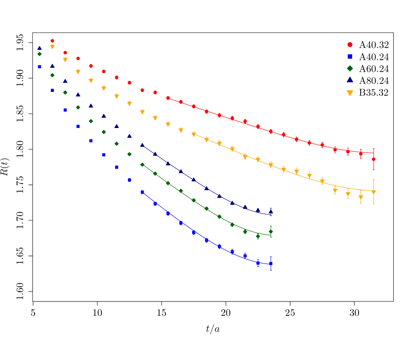
Figure 1: Ratios R(t) as defined in Eq. 15 as a function of $t/a$ for different ensembles in the center of mass frame. We also show the best fit curves for some representatively chosen fit ranges.

Before coming to the actual results, let us first describe our analysis procedure. Statistical errors are always computed using a bootstrap procedure with $R=1500$ bootstrap samples. The bootstrap analysis is chained such that also statistical errors for best fit parameters can be determined. The gauge configurations are sufficiently separated HMC trajectories that autocorrelation does not play a role here, as we explicitly checked using the blocked bootstrap procedure.

Energy shifts are determined from fully correlated fits of the ratios, Eq. 15 to the data. The single pion energy levels needed for the fit are determined from the corresponding two point functions using a one state exponential ($\cosh$) fit to the data, again fully correlated. The correlation between the single pion energy level and the ratio data is taken into account by using the same bootstrap samples.

In figure 1 we show example plots of the ratio for various ensembles. For a representative choice of the fit range we also show the corresponding best fit curves obtained by fitting Eq. 16 to the data. For the fit ranges shown one observes visually a good agreement between fitted curve and data.

The fits to the ratios and the two point functions are repeated for a large number of fit ranges. We then assign a weight

$$w_{\mathrm{X}}=\{(1-2|p_{\mathrm{X}}-0.5|)\cdot\min(\Delta_{\mathrm{X}})/\Delta_{\mathrm{X}}\}^{2}\,,$$ (23)

to every of these fits and quantities $X=E_{\pi},E_{\pi\pi}$, where $p_{\mathrm{X}}$ is the p-value of the corresponding fit and $\Delta_{\mathrm{X}}$ the statistical error of $\langle X\rangle$ determined from the bootstrap procedure.

Figure 2: We show plain, weighted and bootstrap histograms for $M_{\pi}a_{0}$ and the ensembles A40.24 and D45.32, as explained in the text. In the lower left panel we show a QQ-plot for the bootstrap samples quantiles of $M_{\pi}a_{0}$ for A40.24.

Using the weights $w_{X}$, we compute the weighted median over all fit results on the original data to obtain our estimate for the expectation value $\langle X\rangle$. The $68.54\%$ confidence interval of the weighted distribution provides an (not necessarily symmetric) estimate for the systematic uncertainty stemming from the different fit ranges. The statistical error on $\langle X\rangle$ is computed from the $R$ bootstrap samples of the weighted median.

When derived quantities like $q\cot\delta$ are being determined, we follow the same procedure, just that the weights are now given by the products of the weights of the different contributing energy levels.

The fit ranges are chosen such that for both the two point function and the ratio at least five time slices are included in the fit. The two point function is always fitted in an interval $[t_{1}^{\pi},T/2]$ with $t_{1}^{\pi}>6$. For the ratio we fitted in the interval $[t_{1}^{\pi\pi},t_{2}^{\pi\pi}]$ with $t_{1}^{\pi\pi}\in\{11.5,13.5,15.5\}$ and $t_{2}^{\pi\pi}\in\{22.5,21.5,20.5,19.5,18.5\}$ for $L=24,20$ and $t_{2}^{\pi\pi}\in\{30.5,29.5,28.5,26.5,24.5\}$ for $L=32$. We note that due to the weighting procedure described above we could have also included smaller values for $t_{1}^{\pi}$ and $t_{1}^{\pi\pi}$ without affecting the final result.

4.1 Systematic Effects

One of the main issues in this investigation is the question of systematic uncertainties in our analysis procedure. In particular, we have to consider possible contributions by the neutral pion which is much lighter than the charged pion on our ensembles due to twisted mass isospin breaking effects. Possible effects on the $I=2$ pion scattering length extraction have been discussed in detail in Ref. [31].

In Ref. [31] the authors were not able to find evidence of neutral pion contributions within their errors. Even though we have significantly smaller statistical errors, we still do not have any evidence for these effects within the statistical uncertainties. In the pseudo-scalar two point function the possible effect is an excited state with mass $M_{\pi}+M_{\pi^{0}}$ due to the neutral pion having the vacuum quantum numbers in twisted mass lattice QCD [49]. This excited state could, however, never be identified. In the four-point function there can be effects from either close-by excited states at small Euclidean times or thermal states at large Euclidean times. Again, we do not see any evidence of those effects in our data.

However, the analysis procedure detailed above is designed such that such effects should be covered by the systematic error we determine from the weighted distribution. This systematic error mirrors possible deviations from the theoretically expected curve and contributions by excited states or pollutions at large Euclidean times.

The neutral pion might also contribute to the exponential finite size corrections in our data. As discussed below, for $M_{\pi}$ and $f_{\pi}$ we take these twisted mass specific effects into account as determined in Ref. [50] from the data. For $q\cot(\delta_{0})$ finite size corrections specific to twisted mass have not been computed in $\chi$PT and, hence, we can only include the corrections computed in continuum $\chi$PT in Ref. [51]. However, these finite size corrections computed in continuum $\chi$PT have little influence on our results. Hence, we do not expect large effects from twisted mass specific finite size effects.

This conclusion is further supported by the fact that we do not observe large discretisation errors in the results for $M_{\pi}a_{0}$. Any contribution from the neutral pion should show up as a $\mathcal{O}(a^{2})$ lattice artefact. Of course, all these indications are still not enough to finally exclude such systematic effects in our results. But we conclude that within our uncertainties they are negligible.

ens	$a\,\delta E$	$aq\cot\delta_{0}$	$M_{\pi}a_{0}$
A30.32	$0.0037(1)(^{+1}_{-2})$	$-0.92(3)(^{+2}_{-5})$	$-0.133(4)(^{+6}_{-4})$
A40.32	$0.0033(1)(^{+1}_{-1})$	$-0.90(3)(^{+3}_{-2})$	$-0.155(5)(^{+4}_{-3})$
A40.24	$0.0082(3)(^{+4}_{-1})$	$-0.87(3)(^{+5}_{-1})$	$-0.164(5)(^{+2}_{-8})$
A40.20	$0.0179(5)(^{+2}_{-1})$	$-0.71(2)(^{+1}_{-1})$	$-0.202(4)(^{+1}_{-2})$
A60.24	$0.0076(2)(^{+1}_{-1})$	$-0.79(1)(^{+1}_{-1})$	$-0.217(4)(^{+2}_{-3})$
A80.24	$0.0071(1)(^{+0}_{-1})$	$-0.75(1)(^{+0}_{-0})$	$-0.262(3)(^{+1}_{-1})$
A100.24	$0.0063(1)(^{+1}_{-1})$	$-0.75(1)(^{+1}_{-1})$	$-0.294(3)(^{+3}_{-1})$
B55.32	$0.0039(1)(^{+1}_{-1})$	$-0.71(2)(^{+1}_{-1})$	$-0.219(5)(^{+3}_{-2})$
D45.32	$0.0084(2)(^{+0}_{-5})$	$-0.45(1)(^{+0}_{-2})$	$-0.262(6)(^{+12}_{-1})$
B35.32	$0.0041(2)(^{+1}_{-1})$	$-0.82(3)(^{+2}_{-2})$	$-0.151(6)(^{+3}_{-3})$
B85.24	$0.0085(1)(^{+0}_{-1})$	$-0.66(1)(^{+0}_{-1})$	$-0.292(3)(^{+4}_{-1})$

Table 3: $\delta E$, $q\cot\delta_{0}$ and $M_{\pi}a_{0}$ computed with total zero momentum.

4.2 Lüscher formula to $\mathcal{O}(1/L^{5})$

We will discuss several procedures to determine scattering parameters from the data. The first of which is to consider Eq. 17 to the order $1/L^{5}$ and, hence, neglecting the contribution from the effective range, $a_{0}$ can be determined from $\delta E$, $M_{\pi}$ and $L$ by numerically solving Eq. 17 for $a_{0}$. The corresponding results for $a_{0}$ in units of $M_{\pi}$ can be found in table 3.

As an illustration of our analysis procedure we show example histograms in figure 2. With plain histograms we mean histograms of the unweighted results for different fit ranges. In the weighted histograms the weights have been applied according to Eq. 23. And with bootstrap data we denote the median of the weighted distribution evaluated on the bootstrap samples. In the histograms we plot the densities of the distribution.

In the upper left panel the plain and the weighted histogram of $M_{\pi}a_{0}$ determined from Eq. 17 on the A40.24 ensemble are compared. The weighting leads to a well defined peak in the histogram, which is representative for the findings on most ensembles.

In the upper right panel a comparison of the weighted histogram and the histogram of the bootstrap samples of $M_{\pi}a_{0}$ again for A40.24 is shown. That the distribution of the bootstrap samples is approximately normal can be inferred from the lower left panel, where we show the QQ-plot of the bootstrap sample quantiles versus the theoretical quantiles of a standard normal distribution $N_{\bar{\mu},\Delta\mu}$. Here $\bar{\mu}$ is the estimate of $M_{\pi}a_{0}$ and $\Delta\mu$ its statistical error determined from the standard deviation over the bootstrap samples. This comparison indicates that the systematic and statistical uncertainties are approximately of the same size. This finding is again representative for most of the ensembles.

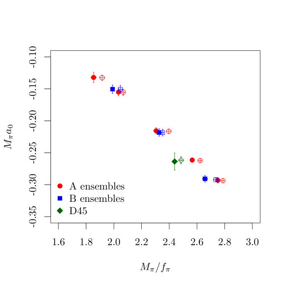
Figure 3: We show finite size corrected data for $M_{\pi}a_{0}$ as a function of $M_{\pi}/f_{\pi}$ with filled symbols compared to uncorrected data with open symbols. The corrected data include also the systematic uncertainty in order to allow for a comparison.

In the lower right panel of figure 2 we show again the plain versus the weighted histogram of $M_{\pi}a_{0}$, but this time for ensemble D45. This ensemble shows the largest systematic uncertainty of all the ensembles investigated here, which is also asymmetric. The weighted median and the systematic uncertainty which are indicated by the circle and the horizontal error bar above the histogram, respectively, show this asymmetry clearly, even if it is not easy to identify by eye.

For the successive analysis we also need to consider (exponentially suppressed) finite size corrections to our data. For $M_{\pi}/f_{\pi}$ and $M_{\pi}$ we use the results of Ref. [50] to correct our data. The corresponding data for $M_{\pi}/f_{\pi}$ and the finite size correction factors are summarised in table 7 in the appendix. We remark that A40.20 and D45.32 have not been considered in Ref. [50]. For D45.32 we use the factors computed in Ref. [50] for ensemble D20.48 with almost identical $M_{\pi}L$-value. For A40.20 we do not need the finite size corrections in the subsequent analyses.

For $a_{0}$ we apply the asymptotic finite size correction formula Eq. (31) from Ref. [13]

$$\begin{split}\Delta(q\cot\delta)&=(q\cot\delta)_{L}-(q\cot\delta)_{L=\infty}\\ &=\frac{-M_{\pi}}{\sqrt{2\pi}}\sum_{n=|\vec{n}|\neq 0}c(n)\frac{e^{-nM_{\pi}L}}{\sqrt{nM_{\pi}L}}\left\{1-\frac{227}{24nM_{\pi}L}+...\right\}\,,\\ \end{split}$$ (24)

which is valid close to threshold (small $q^{2}$) only. The $c(n)$ are multiplicities for the $\vec{n}$ and can be found for instance in Ref. [13]. Note that at zero scattering momentum $\lim_{q\to 0}q\cot\delta=\nicefrac{{1}}{{a_{0}}}$ holds which gives us directly the finite size correction for the scattering length.

For comparison we show the bare data for $M_{\pi}a_{0}$ as a function of $M_{\pi}/f_{\pi}$ with open symbols and the corresponding finite-size corrected data with filled symbols in figure 3. From this plot it is visible that most of the finite-size effects in this analysis stem from the ratio $M_{\pi}/f_{\pi}$. This is because the finite size corrections for $M_{\pi}$ and $f_{\pi}$ are opposite in direction. One can also see the effect of including the systematic uncertainties in the errors, which are included for the finite size corrected data points, but not for the uncorrected ones. This allows one to get an impression of their size and for which ensembles they are actually relevant.

4.3 Lüscher Formula to $\mathcal{O}(1/L^{6})$

We have three A40 ensembles available, which differ only in their spatial extends, $L=20,24$ and $L=32$, respectively. Here, we can apply Eq. 17 in order to estimate the scattering length $a_{0}$ and the effective range $r_{0}$ from the $L$-dependence. It amounts to a fit to the data for $\delta E$ for the three volumes with two fit parameters. For $aM_{\pi}$ we used the values from the largest volume ensemble A40.32. The result is summarised in the first column of table 4.

	$1/L$-fit	$1/L$-fit	$q\cot\delta_{0}$-fit	$q\cot\delta_{0}$-fit
$L$-values	$32,24,20$	$32,24$	$32,24,20$	$32,24$
$a_{0}/a$	$-0.98(5)(^{+2}_{-16})$	$-1.09(7)(^{+20}_{-9})$	$-1.05(3)(^{+1}_{-11})$	$-1.09(6)(^{+9}_{-9})$
$M_{\pi}a_{0}$	$-0.138(6)(^{+2}_{-20})$	$-0.154(10)(^{+28}_{-13})$	$-0.149(4)(^{+1}_{-16})$	$-0.154(8)(^{+12}_{-14})$
$r_{0}/a$	$628(201)$	$42(221)$	$147(22)(^{+30}_{-44})$	$53(107)$
$M_{\pi}r_{0}$	$98(28)$	$6(31)$	$21(3)(^{+4}_{-6})$	$8(15)$
$M_{\pi}^{2}a_{0}r_{0}$	$-87(23)$	$-7(32)$	$-3.1(4)(^{+5}_{-9})$	$-1(2)$
$\chi^{2}/\mathrm{dof}$	$5.14$	-	$0.79$	-

Table 4: A summary of our extractions of the scattering length $a_{0}$, and effective range $r_{0}$ for Lüscher’s $1/L$ expansion of the effective range expansion for two volume combinations each.

According to the $\chi^{2}$ value ($\mathrm{dof}=1$) this is not a good fit. The data for $\delta E$ is shown together with the best fit and an error band in the left panel of figure 4. The result for $M_{\pi}a_{0}$ is lower than the one for the A40.32 ensemble alone (see table 3), but it deviates not more than two $\sigma$. The effective range parameter $r_{0}$ is determined by the fit only with large statistical uncertainties.

It is likely that in particular A40.20 suffers still from exponential finite size artefacts. Therefore, we repeat the analysis with only A40.32 and A40.24 included. Now the fit basically reproduces the result to $\mathcal{O}(1/L^{5})$ of the A40.32 ensemble, and there is no sensitivity to the effective range parameter. The fit result is compiled in table 4 and shown in the right panel of figure 4.

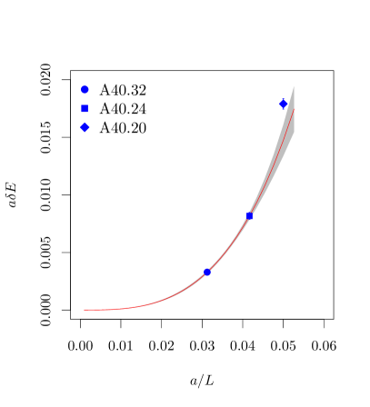
Figure 4: (a) $a\delta E$ as a function of $a/L$ for the three A40 ensembles and the best fit according to Eq. 17. (b) the same like (a) but using A40.32 and A40.24 only.

4.4 Finite Range Expansion for $q\cot\delta_{0}$

Instead of using the expansion in $1/L$ as defined in Eq. 17, one may also determine $q\cot\delta_{0}$ close to threshold directly and perform the effective range expansion as follows:

$$q\,\cot\delta_{0}\ =\ \frac{1}{a_{0}}\ +\ \frac{1}{2}r_{0}q^{2}+\mathcal{O}(q^{4})\,,$$ (25)

where $\delta_{0}$ is the s-wave phase shift, $a_{0}$ the corresponding scattering length, $r_{0}$ the finite range parameter and $q$ the scattering momentum. Using the three ensembles A40.32, A40.24 and A40.20 again, we are able to obtain $q\cot\delta_{0}$ for three values of the squared scattering momentum $q^{2}$. We then apply finite size corrections using Eq. 24.

The corresponding data are shown in the left panel of figure 5 together with the best fit to expression Eq. 25. The statistical error of the fit is indicated by the grey band. In addition, the value extrapolated to $q^{2}=0$ is shown.

The best fit result is summarised in the third column of table 4. In contrast to the fit of the $1/L$ expansion, the finite range expansion provides a good description of $q\cot\delta_{0}$. The $\chi^{2}$-value indicates a good fit, bearing in mind that there is little freedom left. The statistical uncertainties are smaller than the ones obtained from the $1/L$ expansion. In particular, a statistically significant value for the effective range parameter $r_{0}$ is obtained.

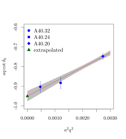
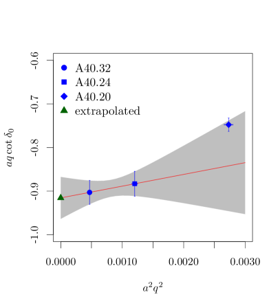
Figure 5: $aq\cot\delta_{0}$ as a function of $a^{2}q^{2}$ for the three ensembles A40.32, A40.24 and A40.20 in (a) and for A40.32 and A40.24 only in (b). In addition the best fit of the effective range expansion to the data is shown as the line and the green triangle indicates the extrapolated value at $q^{2}=0$. The error band indicates the statistical uncertainty of the fit obtained from bootstrapping.

Like in the previous case, where we used Lüscher’s direct method, we also performed an extraction of $a_{0}$ and $r_{0}$ with only the largest two volumes $L=24,32$ with the effective range formula. The result is summarised in the last column of table 4 and the data are shown in the right panel of figure 5. While the scattering length and effective range are in good agreement with previous extractions, we lose statistical significance for $r_{0}$ again. However, the error on $a_{0}$ is only slightly bigger than found for the other three fits. Note that the finite size corrections to $q\cot\delta_{0}$ do not change the fit result significantly.

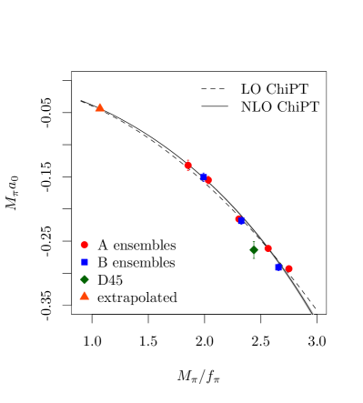
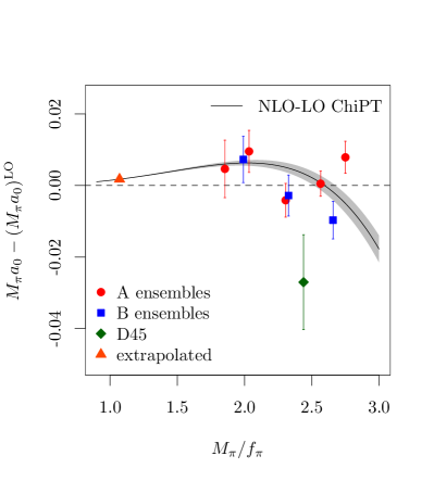
Figure 6: Left: $M_{\pi}a_{0}$ as a function of $M_{\pi}/f_{\pi}$ determined from Eq. 17 to $\mathcal{O}(L^{-5})$ with FS corrections for $M_{\pi}/f_{\pi}$ and $M_{\pi}a_{0}$. The A-ensembles do not include A40.24 and A40.20. We add the LO $\chi$PT prediction as the dashed line. The best fit to the data by the NLO $\chi$PT expression is shown as the solid line with error band. $M_{\pi}a_{0}|_{\mathrm{phys}}$ is plotted as the triangle. Right: the same but with LO $\chi$PT $(M_{\pi}a_{0})^{\mathrm{LO}}$ subtracted.

4.5 Chiral Extrapolation

Because we have determined the scattering parameters for bare quark masses corresponding to larger than physical quark masses, we need to extrapolate to the physical point. For the $I=2$ $\pi\pi$ scattering length $\chi$PT is particularly well suited, because it depends on only one low energy constant at NLO.

As suggested in Refs. [52, 53], it is convenient to write the $\chi$PT expression for $M_{\pi}a_{0}$ as a function of $M_{\pi}/f_{\pi}$, because all quantities are dimensionless and no scale input is needed. The NLO $\chi$PT expression for $M_{\pi}a_{0}$ written as a function of $(M_{\pi}/f_{\pi})$ at a $\chi$PT renormalisation scale $\mu_{R}=f_{\pi,\mathrm{phys}}$ reads [52, 53]

$$M_{\pi}a_{0}=-\frac{M_{\pi}^{2}}{8\pi f_{\pi}^{2}}\left\{1+\frac{M_{\pi}^{2}}{16\pi^{2}f_{\pi}^{2}}\left[3\ln\frac{M_{\pi}^{2}}{f_{\pi}^{2}}-1-\ell_{\pi\pi}(\mu_{R}=f_{\pi,\mathrm{phys}})\right]\right\}$$ (26)

with $\ell_{\pi\pi}$ related to the Gasser-Leutwyler coefficients $\bar{\ell}_{i}$ as follows [54]

$$\ell_{\pi\pi}(\mu_{R})=\frac{8}{3}\bar{\ell}_{1}+\frac{16}{3}\bar{\ell}_{2}-\bar{\ell}_{3}-4\bar{\ell}_{4}+3\ln\frac{M_{\pi,\mathrm{phys}}^{2}}{\mu_{R}^{2}}\,.$$

Moreover, one can show in Twisted mass $\chi$PT that the leading lattice artefacts to $M_{\pi}a_{0}$ are of order $\mathcal{O}(a^{2}M_{\pi}^{2})$ [51]. At NLO we, hence, consistently describe our data with the continuum $\chi$PT formula provided above.

Since we are not (yet) able to determine the pion decay constant $f_{\pi}$ with the sLapH approach, we use data presented in Ref. [55] for the ratio $M_{\pi}/f_{\pi}$ . The values for $M_{\pi}/f_{\pi}$ for all ensembles are compiled in table 7 in the appendix. In this table we also give the values for the finite size correction factors as determined in Ref. [50]. The finite size corrections to $a_{0}$ are analytically computed using Eq. 24 by setting $q\cot\delta_{0}\ =\ \nicefrac{{1}}{{a_{0}}}$. For the finite size corrections of $M_{\pi}$ in $M_{\pi}a_{0}$ we also use the factors compiled in table 7 as discussed above.

The ratio $M_{\pi}/f_{\pi}$ can be determined with significantly smaller uncertainty than $M_{\pi}a_{0}$. Therefore, we do not expect that the missing statistical correlation between $M_{\pi}/f_{\pi}$ and $M_{\pi}a_{0}$ plays any role in the following analysis.

For the fit we propagate the errors on $M_{\pi}/f_{\pi}$ and the finite size corrections on $M_{\pi}$ and $f_{\pi}$ using resampling. For the error on $M_{\pi}a_{0}$ we add the statistical and systematic uncertainty of $M_{\pi}a_{0}$ and the statistical uncertainty of the finite size correction factor $K_{M_{\pi}}$ in quadrature. In the $\chi^{2}$ minimisation we take errors both on $M_{\pi}a_{0}$ and $M_{\pi}/f_{\pi}$ into account. We only include the large volume A40.32 ensemble (and not A40.24 and A40.20) in the fit.

$\ell_{\pi\pi}$	$M_{\pi}a_{0}|_{\mathrm{phys}}$	$\chi^{2}$	$\mathrm{dof}$	p-value	$M_{\pi}/f_{\pi}$-cut
5.13(80)	-0.0437(3)	0.16	2	0.93	2.2
3.94(45)	-0.0441(2)	1.97	4	0.74	2.4
3.68(41)	-0.0442(1)	4.64	5	0.46	2.5
4.73(19)	-0.0438(1)	17.2	8	0.028	-

Table 5: Results from an NLO $\chi$PT fit to our data with different cuts in the upper fit-range.

In the left panel of figure 6 we show the fit to all the data (i.e. with no cut in $M_{\pi}/f_{\pi}$). The solid line represents the best NLO $\chi$PT fit to our data, the dashed line the LO parameter-free $\chi$PT prediction for $M_{\pi}a_{0}$. One observes that the LO $\chi$PT prediction already describes the data surprisingly well, and the NLO fit makes only a small correction to the LO curve. We also show the value of $M_{\pi}a_{0}$ extrapolated to the physical point. In the right panel of figure 6 we show the same, but with the LO $\chi$PT prediction $(M_{\pi}a_{0})^{\mathrm{LO}}$ subtracted.

The data for the A- and B-ensembles fall to a good approximation on a single curve, whereas the only D-ensemble deviates slightly. While not inconsistent with a statistical fluctuation, this might be due to the rather small physical volume of the D45.32 ensemble. Another possible reason might be $a^{2}M_{\pi}^{2}$ lattice artefacts together with higher order terms in continuum $\chi$PT.

We can explore this by restricting the fit range by applying an upper cut in the $M_{\pi}/f_{\pi}$ values. For the case of the fit including only data points with $M_{\pi}/f_{\pi}<2.4$ this is shown in figure 7, which is otherwise identical to figure 6. The cut value is indicated with brackets in the plots.

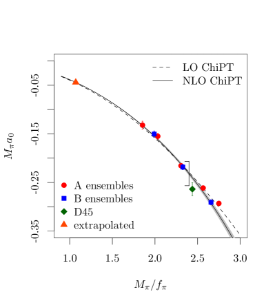
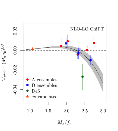
Figure 7: Like figure 6, but for the fit including only data points with $M_{\pi}/f_{\pi}<2.4$ as indicated by the brackets.

The results of the fits to our data with different fit ranges are summarised in table 5. We observe that different fit ranges do have little effect on the extrapolated value of $M_{\pi}a_{0}|_{\mathrm{phys}}$. However, the fit quality improves with decreasing upper fit range, with the best fit for the cuts $M_{\pi}/f_{\pi}<2.4$ and $M_{\pi}/f_{\pi}<2.5$. The only fit parameter $\ell_{\pi\pi}$ shows a large variation, though the fitted values are mostly consistent within errors. The reason for this large variation is visualised in the right panels in figures 6 and 7. The curvature is mainly driven by the points around $M_{\pi}/f_{\pi}=2$. It is also visible that the fitted curves with cut still describe the data reasonably well within errors also for $M_{\pi}/f_{\pi}$ values larger than the applied cut.

As a final result we quote the weighted average of the two fits with cuts $M_{\pi}/f_{\pi}<2.4$ and $M_{\pi}/f_{\pi}<2.5$, respectively

$$M_{\pi}a_{0}\ =\ -0.0442(2)_{\mathrm{stat}}(^{+4}_{-0})_{\mathrm{sys}}\,,\qquad\ell_{\pi\pi}\ =\ 3.79(0.61)_{\mathrm{stat}}(^{+1.34}_{-0.11})_{\mathrm{sys}}\,,$$

with the systematic error estimated from the maximal deviation of the single results in table 5 to the finally quoted one. The uncertainty stemming from the different fit-ranges of the fit to the ratio data turns out to be sub-leading.

5 Discussion

The results presented in the previous section require some discussion. The first important point is that contributions from thermal and excited states as well as the contributions from the neutral pion can be excluded within the statistical uncertainty. With the use of the ratio, Eq. 16, thermal states constant in time are minimised if not cancelled completely. In section 4.2, e.g. figure 2, we show histograms created from fits to a large number of fit ranges. Even for D45 where we see the largest systematic uncertainties stemming from the different fit ranges, the systematic uncertainty is not much bigger than the statistical uncertainty. This lets us conclude that we cannot resolve any of the aforementioned systematic uncertainties within our current statistical precision.

Thanks to the three ensembles A40.32, A40.24 and A40.20 we were able to extract scattering parameters using three different methods: i) $1/L$ expansion, Eq. 17, to the order $1/L^{5}$ for every A40 ensemble separately, ii) the same expansion but to the order $1/L^{6}$ and iii) a direct fit of the effective range expansion to the values of $q\cot\delta_{0}(q^{2})$. Comparing the results in the sections 4.2, 4.3 and 4.4 shows that all three methods give compatible results for $M_{\pi}a_{0}$, apart from method i) for A40.20. The reason for the deviation of method i) for A40.20 can be twofold: on the one hand $M_{\pi}L=2.99$ might be too small and exponentially suppressed finite volume effects cannot be ignored. On the other hand the physical volume might be too small so higher orders in $1/L$ in Lüscher’s formula and higher orders in $q^{2}$ in the effective range expansion are needed. Excluding A40.20 in methods ii) and iii) leads to smaller $M_{\pi}a_{0}$ values, though still compatible within errors to the case when including A40.20. These smaller values, however, are in better agreement to method i) for both A40.32 and A40.24. From this fact alone it is hard to deduce which kind of volume effect we are dealing with here. That the physical volume of A40.20 might be too small is supported by the fact that the D45 ensemble, which is the other ensemble with small physical volume, gives a lower $M_{\pi}a_{0}$ than expected although $M_{\pi}L=3.87$ is in the range of the other ensembles. The important consequence of this finding is that very likely all other ensembles do not suffer from significant finite volume effects. On every other ensemble than A40.20 and D45 the $M_{\pi}L$-value and the physical volume is at least as big as on A40.24 which seems to be free from volume effects within our current precision.

For methods ii) and iii) also the effective range $r_{0}$ can be extracted from fits to the data. The best fit values vary significantly and have mostly very large uncertainties. Only for one fit (see table 4) the $r_{0}$-value is significant. We conclude that at the current level of available data and statistical precision we are not able to reliably extract the effective range parameter.

The chiral extrapolation we present in section 4.5 includes three values of the lattice spacing. The A- and B-ensembles agree quite well, only at larger pion mass values small deviations show up. Unfortunately, we have currently only one ensemble for the smallest lattice spacing value available, namely D45.32. D45.32 has a quite small physical volume, while $M_{\pi}L\approx 3.8$ which is compatible to the other ensembles. Currently, we cannot finally investigate the reason for this discrepancy. It could be a statistical fluctuation, which is supported by the exceptionally large systematic uncertainty for this ensemble, or a finite volume effect, as discussed above. However, we can also not exclude a lattice artifact. We are working on additional D-ensembles, which will allow us to investigate this further.

	$N_{f}$	$M_{\pi}a_{0}$	$\ell_{\pi\pi}$
LO $\chi$PT		$-0.4438$
CGL (2001)		$-0.0444(10)$
CP-PACS (2004)	2	$-0.0431(29)(-)$	$-$
NPLQCD (2006)	2+1	$-0.0426(6)(3)$	$3.3(6)(3)$
NPLQCD (2008)	2+1	$-0.04330(42)_{\mathrm{comb}}$	$6.3(1.2)_{\mathrm{comb}}$
ETM (2010)	2	$-0.04385(28)(38)$	$4.65(0.85)(1.07)$
ETM (2015)	2+1+1	$-0.0442(2)(^{+4}_{-0})$	$3.79(0.61)(^{+1.34}_{-0.11})$
Yagi (2011)	2	$-0.04410(69)(18)$	$5.8(1.2)(-)$
Fu (2013)	2+1	$-0.04430(25)(40)$	$3.27(77)(-)$
PACS-CS (2014)	2+1	$-0.04263(22)(41)$	$-$

Table 6: Compilation of results for $M_{\pi}a_{0}$ and $\ell_{\pi\pi}$ including LO $\chi$PT, $\chi$PT and Roy equations [56] denoted as CGL, CP-PACS [57], NPLQCD (2006) [52], NPLQCD (2008) [30], ETM (2013) [31], this work denoted as ETM (2015), Yagi et al. [58], Fu [59] and PACS-CS [60].

In table 6 we provide a compilation of theoretical determinations for $M_{\pi}a_{0}$ and $\ell_{\pi\pi}$ from the literature: this includes the LO $\chi$PT prediction as well as the value determined using $\chi$PT and Roy equations from Ref. [56] denoted as CGL. For the lattice results we have decided to include only direct determinations for which the chiral extrapolation has been performed: CP-PACS [57], NPLQCD (2006) [52], NPLQCD (2008) [30], ETM (2013) [31], this work denoted as ETM (2015), Yagi et al. [58], Fu [59] and PACS-CS [60]. We quote statistical and – where available – systematic uncertainties separately. For NPLQCD (2008) there is only the combined statistical and systematic uncertainty.

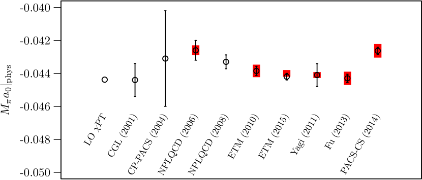
Figure 8: Comparison of the various predictions for $M_{\pi}a_{0}|_{\mathrm{phys}}$. The statistical error is indicated by the error bars on the points, the systematic uncertainty, where available, as coloured bars. Note that for NPLQCD (2008) statistical and systematic errors are combined.

The CP-PACS and the here presented ETM (2015) results are based on three values of the lattice spacing, two have been use by the authors of ETM (2013) and by Fu. The others have used only one value of the lattice spacing, however, NPLQCD (2008) and PACS-CS have used $\chi$PT to estimate discretisation effects. Finite size effects are estimated in the works of NPLQCD (2008), ETM (2013), Yagi et al. and Fu using chiral perturbation theory. In addition to the estimate from chiral perturbation theory we have studied in this work several volumes to obtain an estimate of residual finite volume effects.

As can be observed visually in figure 8, the values for $M_{\pi}a_{0}$ show an overall good agreement. In particular, there is no definite dependence on $N_{f}$. The exception are the high values of NPLQCD (2006) and PACS-CS. PACS-CS quotes in addition a small uncertainty, which makes the deviation to our result statistically significant. If the systematic uncertainty is added to the statistical error, the results are compatible again. PACS-CS has studied the smallest pion mass value around $170\ \mathrm{MeV}$ of all the works considered in this comparison. However, they claim they cannot fit this point with NLO $\chi$PT. Therefore, they had to include higher order terms. More results at close to physical pion mass values might, therefore, clarify whether this is a statistical or systematic effect in the data, or whether the chiral extrapolation with NLO $\chi$PT is misleading.

The values for $\ell_{\pi\pi}$ show a large variation, which is, however, covered by the large errors on this LEC.

6 Summary

In this paper, low-energy $\pi\pi$ scattering in the isospin $I=2$ channel is studied within Lüscher’s finite volume formalism in lattice QCD. We use for the first time $N_{f}=2+1+1$ dynamical quark flavours based on gauge field configurations provided by ETMC. The list of ensembles covers three values of the lattice spacing, several volumes and a large range of pion mass values, see table 1. We determine energy shifts $\delta E=E_{\pi\pi}-2M_{\pi}$ using the stochastic LapH method and convert them in scattering length values applying Lüscher’s formalism.

We apply different, though closely related, methods to determine scattering parameters and find compatible results for $M_{\pi}a_{0}$. The finite range parameter $r_{0}$ cannot be determined with sufficient certainty.

Due to the use of ensembles with a broad range of pion masses we are able to extrapolate $M_{\pi}a_{0}$ towards the physical pion mass point. After correcting for finite volume errors of the scattering length $a_{0}$ we are able to make a rather smooth extrapolation towards the physical pion mass value, the result of which is shown in figure 6. We do not observe significant discretisation effects between A and B-ensembles. The only D-ensemble D45 shows a deviation which can be equally well explained by discretisation effects, finite volume effects or by a statistical fluctuation. To clarify this point, we are generating data on more $D$ ensembles with smaller pion masses.

Our final result for $a^{I=2}_{0}$ is, $M_{\pi}a_{0}\ =\ -0.0442(2)_{\mathrm{stat}}(^{+4}_{-0})_{\mathrm{sys}}$. We have compared our result to a list of other lattice determinations and $\chi$PT combined with Roy equations and found mostly remarkably good agreement.

The currently ongoing extension of the study presented in this paper is $\pi\pi$ scattering with $I=1$, where the $\rho$ resonance is present. With the perambulators ready from the distillation process, this is straightforward to do and first results are available. For the pion-pion scattering, the channel $I=0$ is more complicated, particularly for the twisted mass formulation due to isospin breaking at finite lattice spacing values. Another currently ongoing extension is to address low-energy scattering of other mesons: e.g. $\pi K$ and $KK$ scattering and more than two mesons. Such techniques can also be extended to charmed meson scattering processes relevant for the recently discovered XYZ states.

Acknowledgements

We thank the members of ETMC for the most enjoyable collaboration. The computer time for this project was made available to us by the John von Neumann-Institute for Computing (NIC) on the JUDGE and Juqueen systems in Jülich. We thank U.-G. Meißner for granting us access on JUDGE. We thank A. Rusetsky for very useful discussions. We thank K. Ottnad for providing us with the data for $M_{\pi}/f_{\pi}$ and S. Simula for the estimates of the finite size corrections to $M_{\pi}$ and $f_{\pi}$. We thank C. Michael for helpful comments on the manuscript. This project was funded by the DFG as a project in the Sino-German CRC110. C. Liu, J. Liu and J. Wang are supported in part by the National Science Foundation of China (NSFC) under the project o.11335001. The open source software packages tmLQCD [61], Lemon [62] and R [63] have been used.

Appendix A Data Table

	$aM_{\pi}$	$M_{\pi}/f_{\pi}$	$K_{M_{\pi}}$	$K_{f_{\pi}}$
A30.32	$0.1239(2)(^{+1}_{-1})$	$1.915(10)$	$1.0081(52)$	$0.9757(61)$
A40.32	$0.1415(2)(^{+1}_{-1})$	$2.068(08)$	$1.0039(28)$	$0.9874(24)$
A40.24	$0.1446(3)(^{+1}_{-1})$	$2.202(13)$	$1.0206(95)$	$0.9406(84)$
A40.20	$0.1474(6)(^{+1}_{-2})$	NA	NA	NA
A60.24	$0.1733(3)(^{+5}_{-1})$	$2.396(11)$	$1.0099(49)$	$0.9716(37)$
A80.24	$0.1993(2)(^{+1}_{-0})$	$2.623(07)$	$1.0057(29)$	$0.9839(22)$
A100.24	$0.2224(2)(^{+2}_{-0})$	$2.788(07)$	$1.0037(19)$	$0.9900(15)$
B35.32	$0.1249(2)(^{+1}_{-1})$	$2.047(11)$	$1.0069(32)$	$0.9794(27)$
B55.32	$0.1555(2)(^{+1}_{-1})$	$2.352(07)$	$1.0027(14)$	$0.9920(10)$
B85.24	$0.1933(3)(^{+0}_{-1})$	$2.736(15)$	$1.0083(28)$	$0.9795(24)$
D45.32	$0.1207(3)(^{+1}_{-1})$	$2.485(12)$	$1.0047(14)$	$0.9860(13)$

Table 7: Single pion energy levels, $M_{\pi}/f_{\pi}$ and the finite size correction factors $K_{M_{\pi}}$ and $K_{f_{\pi}}$ computed in Ref. [50] for $M_{\pi}$ and $f_{\pi}$, respectively.

References

- [1] L. Maiani and M. Testa, Phys.Lett. B245, 585 (1990).
- [2] M. Lüscher, Commun.Math.Phys. 104, 177 (1986).
- [3] M. Lüscher, Commun.Math.Phys. 105, 153 (1986).
- [4] M. Lüscher and U. Wolff, Nucl.Phys. B339, 222 (1990).
- [5] M. Lüscher, Nucl.Phys. B354, 531 (1991).
- [6] K. Rummukainen and S. A. Gottlieb, Nucl.Phys. B450, 397 (1995), arXiv:hep-lat/9503028.
- [7] C. Kim, C. Sachrajda, and S. R. Sharpe, Nucl.Phys. B727, 218 (2005), arXiv:hep-lat/0507006.
- [8] ETM, X. Feng, K. Jansen, and D. B. Renner, PoS LATTICE2010, 104 (2010), arXiv:1104.0058.
- [9] M. Gockeler et al., Phys.Rev. D86, 094513 (2012), arXiv:1206.4141.
- [10] X. Li and C. Liu, Phys. Lett. B587, 100 (2004), arXiv:hep-lat/0311035.
- [11] X. Feng, X. Li, and C. Liu, Phys. Rev. D70, 014505 (2004), arXiv:hep-lat/0404001.
- [12] W. Detmold and M. J. Savage, Nucl.Phys. A743, 170 (2004), arXiv:hep-lat/0403005.
- [13] P. F. Bedaque, I. Sato, and A. Walker-Loud, Phys.Rev. D73, 074501 (2006), arXiv:hep-lat/0601033.
- [14] M. Doring, U.-G. Meissner, E. Oset, and A. Rusetsky, Eur.Phys.J. A47, 139 (2011), arXiv:1107.3988.
- [15] R. A. Briceno, Z. Davoudi, T. C. Luu, and M. J. Savage, Phys.Rev. D89, 074509 (2014), arXiv:1311.7686.
- [16] D. Agadjanov, U.-G. Mei?ner, and A. Rusetsky, JHEP 1401, 103 (2014), arXiv:1310.7183.
- [17] S. He, X. Feng, and C. Liu, JHEP 0507, 011 (2005), arXiv:hep-lat/0504019.
- [18] C. Liu, X. Feng, and S. He, Int.J.Mod.Phys. A21, 847 (2006), arXiv:hep-lat/0508022.
- [19] V. Bernard, M. Lage, U.-G. Meissner, and A. Rusetsky, JHEP 1101, 019 (2011), arXiv:1010.6018.
- [20] M. T. Hansen and S. R. Sharpe, Phys.Rev. D86, 016007 (2012), arXiv:1204.0826.
- [21] R. A. Briceno and Z. Davoudi, Phys.Rev. D88, 094507 (2013), arXiv:1204.1110.
- [22] P. Guo, J. Dudek, R. Edwards, and A. P. Szczepaniak, Phys.Rev. D88, 014501 (2013), arXiv:1211.0929.
- [23] L. Roca and E. Oset, Phys.Rev. D85, 054507 (2012), arXiv:1201.0438.
- [24] K. Polejaeva and A. Rusetsky, Eur.Phys.J. A48, 67 (2012), arXiv:1203.1241.
- [25] R. A. Briceno and Z. Davoudi, Phys.Rev. D87, 094507 (2013), arXiv:1212.3398.
- [26] M. T. Hansen and S. R. Sharpe, (2013), arXiv:1311.4848.
- [27] M. T. Hansen and S. R. Sharpe, (2015), arXiv:1504.04248.
- [28] M. T. Hansen and S. R. Sharpe, (2014), arXiv:1409.7012.
- [29] M. T. Hansen and S. R. Sharpe, Phys.Rev. D90, 116003 (2014), arXiv:1408.5933.
- [30] S. R. Beane et al., Phys.Rev. D77, 014505 (2008), arXiv:0706.3026.
- [31] X. Feng, K. Jansen, and D. B. Renner, Phys.Lett. B684, 268 (2010), arXiv:0909.3255.
- [32] J. J. Dudek, R. G. Edwards, M. J. Peardon, D. G. Richards, and C. E. Thomas, Phys.Rev. D83, 071504 (2011), arXiv:1011.6352.
- [33] NPLQCD, S. Beane et al., Phys.Rev. D85, 034505 (2012), arXiv:1107.5023.
- [34] J. J. Dudek, R. G. Edwards, and C. E. Thomas, Phys.Rev. D86, 034031 (2012), arXiv:1203.6041.
- [35] S. Prelovsek, PoS LATTICE2014, 015 (2014), arXiv:1411.0405.
- [36] ALPHA, R. Frezzotti, P. A. Grassi, S. Sint, and P. Weisz, JHEP 08, 058 (2001), hep-lat/0101001.
- [37] R. Frezzotti and G. C. Rossi, JHEP 08, 007 (2004), hep-lat/0306014.
- [38] ETM, R. Baron et al., JHEP 06, 111 (2010), arXiv:1004.5284.
- [39] ETM, R. Baron et al., Comput.Phys.Commun. 182, 299 (2011), arXiv:1005.2042.
- [40] R. Frezzotti and G. C. Rossi, Nucl. Phys. Proc. Suppl. 128, 193 (2004), hep-lat/0311008.
- [41] T. Chiarappa et al., Eur.Phys.J. C50, 373 (2007), arXiv:hep-lat/0606011.
- [42] Hadron Spectrum, M. Peardon et al., Phys. Rev. D80, 054506 (2009), arXiv:0905.2160.
- [43] C. Morningstar et al., Phys.Rev. D83, 114505 (2011), arXiv:1104.3870.
- [44] A. Hasenfratz and F. Knechtli, Phys.Rev. D64, 034504 (2001), arXiv:hep-lat/0103029.
- [45] C. Michael and I. Teasdale, Nucl.Phys. B215, 433 (1983).
- [46] M. Fukugita, Y. Kuramashi, M. Okawa, H. Mino, and A. Ukawa, Phys.Rev. D52, 3003 (1995), arXiv:hep-lat/9501024.
- [47] T. Umeda, Phys.Rev. D75, 094502 (2007), arXiv:hep-lat/0701005.
- [48] S. R. Beane, W. Detmold, and M. J. Savage, Phys.Rev. D76, 074507 (2007), arXiv:0707.1670.
- [49] A. Shindler, Phys.Rept. 461, 37 (2008), arXiv:0707.4093.
- [50] ETM, N. Carrasco et al., Nucl.Phys. B887, 19 (2014), arXiv:1403.4504.
- [51] M. I. Buchoff, J.-W. Chen, and A. Walker-Loud, Phys.Rev. D79, 074503 (2009), arXiv:0810.2464.
- [52] NPLQCD, S. R. Beane, P. F. Bedaque, K. Orginos, and M. J. Savage, Phys.Rev. D73, 054503 (2006), arXiv:hep-lat/0506013.
- [53] NPLQCD, S. R. Beane et al., Phys.Rev. D77, 094507 (2008), arXiv:0709.1169.
- [54] J. Bijnens, G. Colangelo, G. Ecker, J. Gasser, and M. Sainio, Nucl.Phys. B508, 263 (1997), arXiv:hep-ph/9707291.
- [55] ETM, C. Michael, K. Ottnad, and C. Urbach, Phys.Rev.Lett. 111, 181602 (2013), arXiv:1310.1207.
- [56] G. Colangelo, J. Gasser, and H. Leutwyler, Nucl.Phys. B603, 125 (2001), arXiv:hep-ph/0103088.
- [57] CP-PACS, T. Yamazaki et al., Phys. Rev. D70, 074513 (2004), arXiv:hep-lat/0402025.
- [58] T. Yagi, S. Hashimoto, O. Morimatsu, and M. Ohtani, (2011), arXiv:1108.2970.
- [59] Z. Fu, Phys.Rev. D87, 074501 (2013), arXiv:1303.0517.
- [60] PACS-CS, K. Sasaki, N. Ishizuka, M. Oka, and T. Yamazaki, Phys.Rev. D89, 054502 (2014), arXiv:1311.7226.
- [61] K. Jansen and C. Urbach, Comput.Phys.Commun. 180, 2717 (2009), arXiv:0905.3331.
- [62] ETM, A. Deuzeman, S. Reker, and C. Urbach, (2011), arXiv:1106.4177.
- [63] R Development Core Team, R: A language and environment for statistical computing, R Foundation for Statistical Computing, Vienna, Austria, 2005, ISBN 3-900051-07-0.