Engineering flat electronic bands in quasiperiodic and fractal loop geometries

Abstract

Exact construction of one electron eigenstates with flat, non-dispersive bands, and localized over clusters of various sizes is reported for a class of quasi-one dimensional looped networks. Quasiperiodic Fibonacci and Berker fractal geometries are embedded in the arms of the loop threaded by a uniform magnetic flux. We work out an analytical scheme to unravel the localized single particle states pinned at various atomic sites or over clusters of them. The magnetic field is varied to control, in a subtle way, the extent of localization and the location of the flat band states in energy space. In addition to this we show that, an appropriate tuning of the field can lead to a re-entrant behavior of the effective mass of the electron in a band, with a periodic flip in its sign.

Geometrically frustrated lattices (GFL) supporting flat, dispersionless bands in their energy spectrum with macroscopically degenerate eigenstates have drawn great interest in recent times derzhko -flach3 . Initial interest in antiferromagnetic Heisenberg model on frustrated lattices  kikuchi -moessner has evolved into extensive studies of the gapped flat band states to gapless chiral modes in graphenes yao , in optical lattices of ultracold atoms bloch , waveguide arrays christo , or in microcavities having exciton-polaritons masumoto . The quenched kinetic energy of an electron in a flat band state (FBS) leads to the possibility of achieving strongly correlated electronic states, topologically ordered phases, such as the lattice versions of fractional quantum Hall states  liu . Recently, the controlled growth of artificial lattices with complications such as in the kagomé class has added excitement to such studies guzman - tamura .

Spinless fermions are easily trapped in flat bands mati . The non-dispersive character of the energy ($E$)- wave vector ($k$) curve implies an infinite effective mass of the electron, leading to practically its immobility in the lattice. Such states are therefore strictly localized either on special sets of vertices, or in a finite cluster of atomic sites spanning finite areas of the underlying lattice. Recently it has been shown that, an infinity of such cluster-localized single particle states can be exactly constructed even in a class of deterministic fractals atanu . Apart from its interest in direct relation to the study of GFL’s, this work provides an example where eigenvalues corresponding to localized eigenstates in an infinite fractal geometry can be exactly evaluated, a task that is a non-trivial one if one remembers that these fractal systems are free from translational invariance of any kind.

In this communication we unravel and analyze groups of flat, dispersionless energy bands in some tailor made GFL’s. The lattices display an interesting competition between long range translational order along the horizontal ($x-$) axis and an aperiodic growth in the

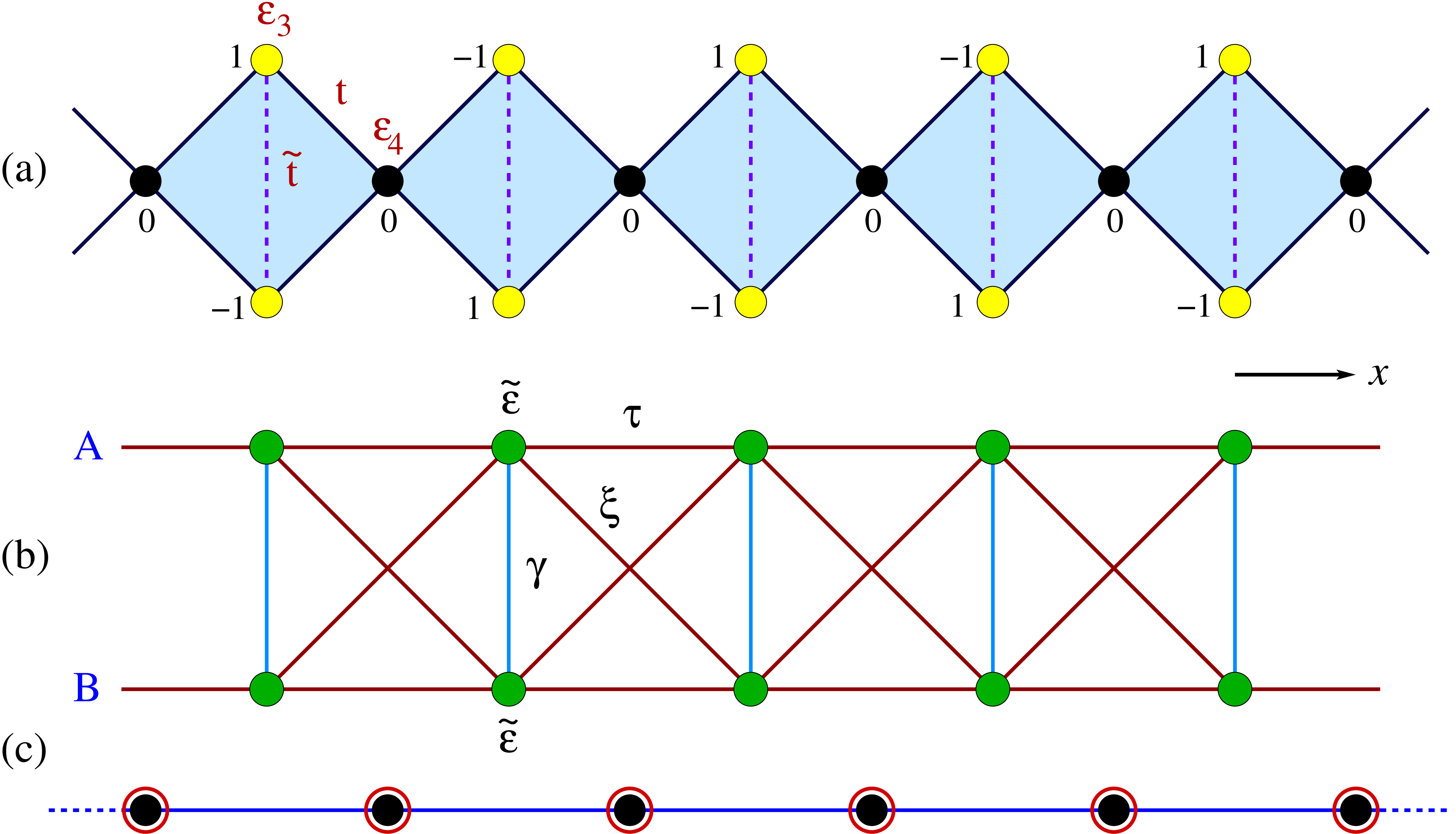
Figure 1: (Color online). (a) A typical realization of an elementary array of diamond shaped quadruplets exhibiting a single flat, dispersionless band at $E=0$, (b) its renormalization into an effective two-arm ladder network with energy dependent potential and nearest and next nearest neighbor interactions and, (c) the effective one dimensional chain obtained after decimating out the top (yellow colored) vertices.

transverse directions. In each case, the skeleton is an infinite array of diamond shaped networks (Fig. 1(a)) where hierarchical structures, grown deterministically, are embedded in each arm of the diamond. A uniform magnetic flux threads each elementary plaquette, as will be illustrated in appropriate cases. The motivation behind the present study is two fold.

First, exploiting the self similar growth of the hierarchical structures we can implement a real space renormalization group (RSRG) scheme to evaluate the pinned, flat band states (FBS) exactly. In all the cases we discuss in this paper the flat band states merge with the localized eigenstates of the infinite hierarchical geometry as higher and higher generations of them are embedded in the arms of the underlying diamonds. Thus, once again, the problem of an exact evaluation of localized states in a fractal geometry is, at least partially, solved.

Second, and a more important aspect of the problem is to look for a possible coexistence of a multitude of dispersive and non-dispersive energy bands in a periodic array of the elementary building blocks. As an arm of the elementary diamond hosts a quasi-periodic or a deterministic fractal of sequentially increasing generation, the flat, dispersive bands are likely get densely packed in an environment of dispersive ones. The density of packing may even lead, for a large enough generation of the hierarchical structure, to a re-entrant dispersive to non-dispersive crossover in the behavior of the electrons. A recent inspiring work by Danieli et al. flach3 has shown that a quasiperiodically modulated flat band geometry may even allow for a precise engineering of the mobility edges.

In addition to this, we anticipate that, a variation in the strength of the magnetic field can lead to a tuning of the curvature of the energy dispersion curves. We can thus achieve a comprehensive control over the group velocity and effective mass of the electron with the help of an external field. Knowing that, a deterministic quasiperiodic or fractal geometry normally offers a completely fragmented, Cantor set-like energy spectrum, this latter study may allow us to control the effective mass of the electron using an external agent such as the magnetic field over arbitrarily small scales of the energy or, equivalently, the wave vector.

We present here a simple analytical method to detect the sharply localized eigenstates that are pinned on certain atoms or atomic clusters in a periodic array of diamonds. The non-dispersive character of such states is explicitly worked out. The method is then extended to unravel the entire set of such FBS when each arm of an elementary diamond hosts a quasiperiodic lattice grown according to a deterministic Fibonacci sequence sutherland , and Berker griffiths geometry. Such aperiodic structures with sequentially increasing hierarchy are embedded in the diamond’s arm. We indeed find that, as one gradually increases the degree of aperiodicity in the arms, the pinned FBS in such periodic approximants turn out to be the localized eigenstates of the systems in their respective thermodynamic limits.

In addition, we observe that, with a deterministic aperiodic geometry of sufficiently large generation embedded in the arms of a diamond array, the interplay of periodicity along the $x$-axis and the aperiodic order in the transverse directions, produces a highly complex dispersion pattern. The flat, dispersionless bands densely fill the gaps between the dispersive ones, giving rise to the possibility of a quasi-continuous crossover between them as the aperiodic components grow in hierarchy.

The magnetic field piercing the elementary plaquettes in each case is shown to control the group velocity of the electrons, making them more and more immobile as the flux $\Phi\rightarrow\Phi_{0}/2$, where $\Phi_{0}=hc/e$ is the fundamental flux quantum. This is an exemplary case of extreme localization induced by the magnetic flux as discussed by Vidal and co-workers  vidal1 -vidal3 . The magnetic field is shown to flip the sign of the effective mass multiple times within a single Brillouin zone - a remarkable contrast to the ordinary periodic linear lattice. The electron-lattice interaction thus can be fine tuned from outside by selective choice of the flux threading a plaquette.

In what follows, we present our results. In section I we work out the basic method of analyzing the FBS in an elementary diamond array, and compare the result with the existing ones. Section II deals with the Fibonacci-diamond chain, and in section III we elaborately discuss the fractal-diamond networks. In section IV we explicitly discuss the generic diamond loop-array where a magnetic field controls the effective mass of the electron making its sign periodically flipped. In section V we draw our conclusions.

I The Hamiltonian and the pinned eigenstates

We refer to Fig. 1. Spinless, non-interacting electrons are described using a tight-binding hamiltonian in the Wannier basis, viz.,

$$H=\sum_{i}\epsilon_{i}c_{i}^{\dagger}c_{i}+\sum_{\langle ij\rangle}t_{ij}\left[c_{i}^{\dagger}c_{j}+h.c.\right]$$ (1)

where, $\epsilon_{i}$ is the on-site potential and can assume values equal to $\epsilon_{3}$ or $\epsilon_{4}$ depending on the site at the vertex having a coordination number $z=3$ (yellow circles), or in the bulk, having a coordination number $z=4$ (black circles). Throughout this paper we shall choose $\epsilon_{3}=\epsilon_{4}$ just to see the effect of the topology of the lattice alone. However, the symbols will be in use to facilitate any discussion. The nearest neighbor hopping integral $t_{ij}=t$ along the arm of the diamond, and $t_{ij}=\tilde{t}$ along the diagonal connecting the vertices with coordination number two. The Schrödinger equation, written equivalently in the form of the difference equation,

$$(E-\epsilon_{i})\psi_{i}=\sum_{j}t_{ij}\psi_{j}$$ (2)

allows us to decimate out the “black” vertices of the diamond network to map the original array on to an effective two-arm ladder (Fig. 1(b)) (with arms marked $A$ and $B$) comprising identical (green colored) atomic sites with renormalized on-site potential $\tilde{\epsilon}=\epsilon_{3}+2t^{2}/(E-\epsilon_{4})$. The renormalized hopping integral along the arm of the ladder now becomes $\tau=t^{2}/(E-\epsilon_{4})$, and the inter-arm hopping becomes $\gamma=\tilde{t}+2t^{2}/(E-\epsilon_{4})$. The decimation generates a second neighbor hopping (brown line) inside a unit plaquette of the ladder and along the diagonal, viz., $\xi=t^{2}/(E-\epsilon_{4})$.

The difference equation for the ladder network may now be cast using $2\times 2$ matrices, in the form sil :

$$\left[\left(\begin{array}[]{cccc}E&0\\ 0&E\end{array}\right)-\left(\begin{array}[]{cccc}\tilde{\epsilon}&\gamma\\ \gamma&\tilde{\epsilon}\end{array}\right)\right]\left(\begin{array}[]{c}\psi_{n,A}\\ \psi_{n,B}\end{array}\right) = \left(\begin{array}[]{cccc}\tau&\xi\\ \xi&\tau\end{array}\right)\left(\begin{array}[]{c}\psi_{n+1,A}\\ \psi_{n+1,B}\end{array}\right)+\left(\begin{array}[]{cccc}\tau&\xi\\ \xi&\tau\end{array}\right)\left(\begin{array}[]{c}\psi_{n-1,A}\\ \psi_{n-1,B}\end{array}\right)$$ (17)

It is easy to check that both the ‘potential matrix’ (comprising $\tilde{\epsilon}$ and $\gamma$) and the ‘hopping matrix’ (with $\tau$ and $\xi$) commute, and hence can be simultaneously diagonalized by a similarity transform. Eq. (17) can then be easily decoupled, in a new basis defined by $\phi_{n}=\mathbf{M}^{-1}\psi_{n}$. The matrix $\mathbf{M}$ diagonalizes both the ‘potential’ and the ‘hopping’ matrices. The decoupled set of equations are free from any ‘cross terms’ and reads, in terms of the original on-site potentials and hopping integrals, as:

$$\left[E-\left(\epsilon_{3}+\tilde{t}+\frac{4t^{2}}{E-\epsilon_{4}}\right)\right]\phi_{n,A} = \frac{2t^{2}}{E-\epsilon_{4}}(\phi_{n+1,A}+\phi_{n-1,A})$$

$$(E-\epsilon_{3}+\tilde{t})\phi_{n,B} = 0$$ (18)

The first equation represents a periodic array of identical atomic sites with renormalized on-site potential $\epsilon_{3}+\tilde{t}+4t^{2}/(E-\epsilon_{4})$, and nearest neighbor hopping integral $2t^{2}/(E-\epsilon_{4})$. The second equation in Eq. (18) represents (in the new basis) an effective atom, decoupled from its neighbors. The potential of this isolated atomic site is $\epsilon_{3}-\tilde{t}$. This leads to an eigenfunction with amplitudes pinned at the $z=3$ vertices as shown in Fig. 1(a) and the corresponding eigenvalue is at $E=\epsilon_{3}-\tilde{t}$. The amplitude $\psi_{i}=0$ at all the $z=4$ vertices for this special energy. The non-zero amplitudes are thus trapped in local clusters ($z=3$ vertices), as discussed in the introduction. The result obtained by Hyrkäs et al. mati identifies this state as a flat, non-dispersive one comment .

To confirm the non-dispersive character of this pinned eigenstate, we refer to Fig. 1(c), where an effective linear chain of identical atoms is obtained by decimating the $\epsilon_{3}$ vertices. The resulting on-site potential and the nearest neighbor hopping integral for this linear lattice is given by,

$$\epsilon_{0} = \epsilon_{4}+\frac{4t^{2}(E-\epsilon_{3}+\tilde{t})}{(E-\epsilon_{3})^{2}-\tilde{t}^{2}}$$

$$t_{0} = \frac{2t^{2}(E-\epsilon_{3}+\tilde{t})}{(E-\epsilon_{3})^{2}-\tilde{t}^{2}}$$ (19)

The linear chain described by Eq. (19) has a dispersion relation,

$$(E-\epsilon_{3}+\tilde{t})\left[(E-\epsilon_{4})(E-\epsilon_{3}-\tilde{t})-8\tilde{t}^{2}\cos^{2}\left(\frac{ka}{2}\right)\right]=0$$ (20)

In the above equation $a$ is the lattice constant of the effective periodic chain. Eq. (20) clearly indicates a non-dispersive, wave vector-independent, flat band at $E=\epsilon_{3}-\tilde{t}$. This is compliant with the result obtained by analyzing the decoupled set of equations Eq. (18). The same set of arguments brings back the FBS at $E=\epsilon_{3}$ as shown in ref mati for $\epsilon_{3}=0$.

II The Fibonacci-Diamond array

We now construct a periodic array of diamond with a Fibonacci segment of two different bond lengths $L$ and $S$ embedded in it. The linear Fibonacci chain grows according to the prescription sutherland $L\rightarrow LS$ and $S\rightarrow L$. This generates a quasiperiodic chain with two different hopping integrals, viz., $t_{L}$ and $t_{S}$ and three kinds of vertices $\alpha$ (flanked by two $L$-bonds), $\beta$ ($L$ on the left and $S$ on the right), and $\gamma$ (in between an $S-L$ pair). The corresponding on-site potentials are designated by $\epsilon_{\alpha}$, $\epsilon_{\beta}$ and $\epsilon_{\gamma}$ respectively. Fig. 2 describes a periodic array of diamonds with each arm hosting a third generation Fibonacci segment $LSL$. A magnetic flux pierces each diamond. The hopping integrals along the bonds $L$ and $S$ pick up Peierls’ phases vidal1 , and read $t_{L}^{f(b)}=t_{L}\exp(\pm i\theta_{L})$ and $t_{S}^{f(b)}=t_{S}\exp(\pm i\theta_{S})$ respectively. Here, $\theta_{L(S)}=2\pi\Phi a_{L(S)}/(F_{n-1}a_{L}+F_{n-2}a_{S})$, $F_{n}$ being the Fibonacci number in the $n$-th generation. The symbols $f$ and $b$ refer to the hopping in the so called forward and backward directions respectively - a consequence of the broken time reversal symmetry.

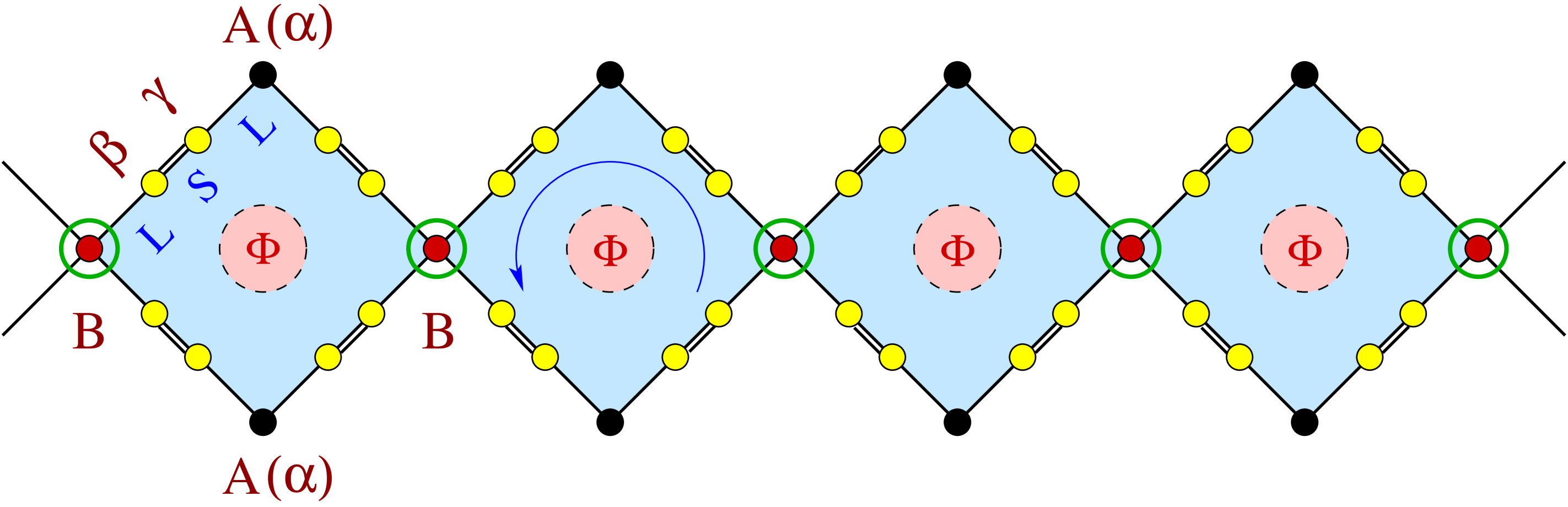
Figure 2: (Color online). (a) A perfectly periodic array of identical diamond blocks when each arm of a diamond hosts a third generation Fibonacci sequence of bonds $L$ and $S$.

In what follows, we shall deal with generations ending with the $L$ bond only, that is, $G_{2n+1}$, $n=1$, $2$, $.........$. This is only for convenience, and does not affect the final result as we are interested in the case when $n\rightarrow\infty$.

As proposed, we embed a $(2n+1)$-th generation Fibonacci segment in each arm of the diamond. The difference equations Eq. (2) for the three kinds of atomic sites are now of the form,

$$(E-\epsilon_{\alpha})\psi_{j} = t_{L}e^{i\theta_{L}}\psi_{j+1}+t_{L}e^{-i\theta_{L}}\psi_{j-1}$$

$$(E-\epsilon_{\beta})\psi_{j} = t_{S}e^{i\theta_{S}}\psi_{j+1}+t_{L}e^{-i\theta_{L}}\psi_{j-1}$$

$$(E-\epsilon_{\gamma})\psi_{j} = t_{L}e^{i\theta_{L}}\psi_{j+1}+t_{S}e^{-i\theta_{S}}\psi_{j-1}$$ (21)

where, the index $j$ refers to a site of type $\alpha$, $\beta$ or $\gamma$ appropriately.

The Fibonacci segment trapped in a diamond arm is now decimated $n$ times, using the set of Eq. (21) to reduce the geometry into a simple diamond with

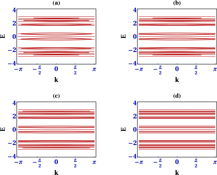
Figure 3: (Color online) Dispersion curves for a 5th generation Fibonacci-Diamond array for (a) $\Phi=0$, (b) $\Phi=\Phi_{0}/4$, (c) $\Phi=2\Phi_{0}/5$, and (d) $\Phi=\Phi_{0}/2$. We have chosen $\epsilon_{\alpha}=\epsilon_{\beta}=\epsilon_{\gamma}=0$, $t_{L}=1$ and $t_{S}=2$. Energy is measured in units of $t_{L}$.

two kinds of vertices with renormalized on site potentials $\epsilon_{\alpha,n}$, (black dots) and $\epsilon_{c,n}$ (red dots encircled with green line). The effective hopping integral connecting these two sites is $t_{L,n}^{f(b)}$, depending on the sense of traversal. The recursion relations we exploit during the sequential decimation process are given by,

$$\epsilon_{\alpha,n} = \epsilon_{\alpha,n-1}+\frac{t_{L,n-1}^{f}t_{L,n-1}^{b}[2E-(\epsilon_{\beta,n-1}+\epsilon_{\gamma,n-1})]}{\Delta_{n-1}}$$

$$\epsilon_{\beta,n} = \epsilon_{\alpha,n-1}+\frac{(E-\epsilon_{\beta,n-1})t_{L,n-1}^{f}t_{L,n-1}^{f}}{\Delta_{n-1}}+\frac{t_{L,n-1}^{f}t_{L,n-1}^{b}}{E-\epsilon_{\beta,n-1}}$$

$$\epsilon_{\gamma,n} = \epsilon_{\gamma,n-1}+\frac{(E-\epsilon_{\gamma,n-1})t_{L,n-1}^{f}t_{L,n-1}^{b}}{\Delta_{n-1}}+\frac{t_{S,n-1}^{f}t_{S,n-1}^{b}}{E-\epsilon_{\beta,n-1}}$$

$$\epsilon_{c,n} = \epsilon_{\alpha,n-1}+2\left[\frac{t_{L,n-1}^{f}t_{L,n-1}^{b}[2E-(\epsilon_{\beta,n-1}+\epsilon_{\gamma,n-1})]}{\Delta_{n-1}}\right]$$

$$t_{L,n}^{f} = \frac{(t_{L,n-1}^{f})^{2}t_{S,n-1}^{f}}{\Delta_{n-1}}$$

$$t_{S,n}^{f} = \frac{t_{L,n-1}^{f}t_{S,n-1}^{f}}{E-\epsilon_{\beta,n-1}}$$ (22)

Obviously, $t_{L(S),n}^{b}=t_{L(S),n}^{f*}$ at any $n$-th stage of renormalization. The quantity $\Delta_{n}$ is given by $\Delta_{n}=(E-\epsilon_{\beta,n})(E-\epsilon_{\gamma,n})-t_{S,n}^{f}t_{S,n}^{b}$.

As the Fibonacci segment is decimated completely following an $n$ step execution of the recursion relations (22), the Fibonacci-diamond geometry is reduced to a

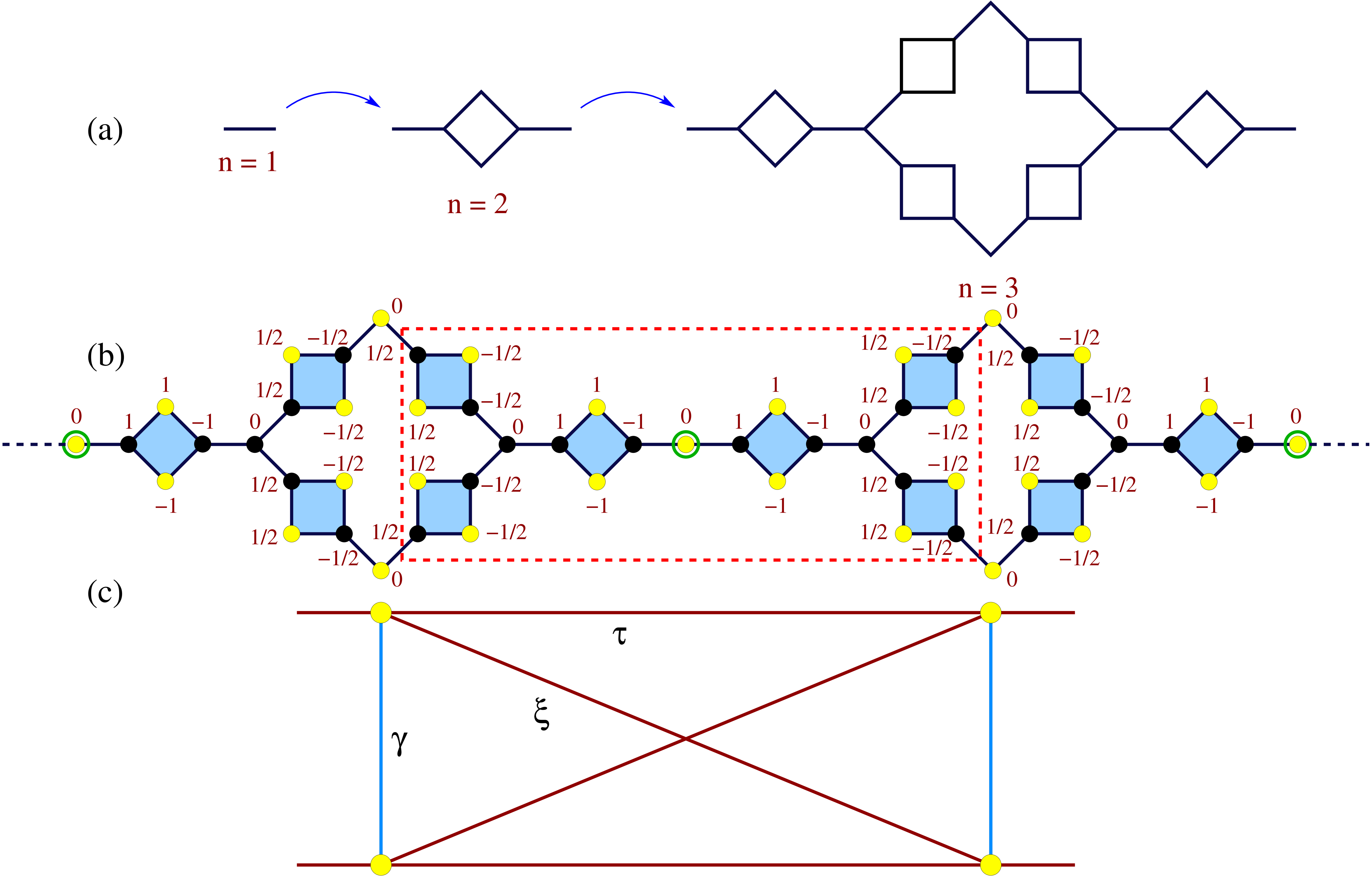
Figure 4: (Color online) (a) Construction of an open Berker-diamond chain. (b) Distribution of amplitudes $\psi_{i}$ for a flat band at $E=\epsilon_{2}=0$. We have set $t=1$. (c) Conversion of an open Berker-diamond array into a two arm ladder network.

simple diamond array, as shown in Fig. 1 with $\epsilon_{\alpha,n}$ and $\epsilon_{c,n}$ playing the roles of $\epsilon_{3}$ and $\epsilon_{4}$ in Eq. (19) respectively. Obviously, $t_{L,n}$ now replaces $t$ and $\tilde{t}=0$. The simple analogy reveals that, we have localized eigenstates pinned at the effective $\alpha$ sites (by virtue of the second equation in Eq. (18)) for all energy eigenvalues obtained by solving the equation $E-\epsilon_{\alpha,n}=0$. The corresponding dispersion relation, in analogy with Eq. (19) is given by,

$$(E-\epsilon_{\alpha,n})\left[(E-\epsilon_{c,n})(E-\epsilon_{\alpha,n})-8t_{L,n}^{2}\cos^{2}\left(\frac{ka}{2}\right)\right]=0$$ (23)

The flat, non-dispersive $k$-independent bands are easily seen to originate from the solution of the equation $E-\epsilon_{\alpha,n}=0$.

The solutions of the equation $E=\epsilon_{\alpha,n}$ constitute the eigenvalue spectrum of a Fibonacci chain samar as $n\rightarrow\infty$. The spectrum exhibits a global three subband structure. Each subband can be scanned over finer scales of the wave vector to bring out the inherent self similarity and multifractality, the hallmark of the Fibonacci quasicrystals sutherland . In the Fibonacci diamond array, we encounter precisely this feature, as already evident from Fig. 3. Each of the three subbands are populated by the dispersive as well as the non-dispersive FBS. The self similarity of the bands have been checked by going over to higher generations, though we refrain from showing these data to save space here.

In the limit $n\rightarrow\infty$, that is, when a single diamond arm hosts an infinitely large Fibonacci segment, the dispersive and non-dispersive bands get more and more densely packed, and if one travels along a vertical line at a fixed value of the wave vector, a dispersive (non-dispersive) to non-dispersive (dispersive) crossover within a single sub-cluster of states is likely to be observed. Needless to say, such a crossover can take place over an arbitrarily small interval $\Delta k$ of the wave vector. In Fig. 3 we have shown the bands for a pure transfer model sutherland , where the on-site potentials are set equal to zero, and the quasiperiodic order is built in the distribution of the hopping integrals only. The central state at $E=0$ is there for all values of the flux, and as we have checked, for all generations. This state belongs to the spectrum of an infinite Fibonacci chain, as is well known in the existing literature sutherland .

A magnetic field is found to flatten the dispersive bands, decreasing the group velocity, and finally leading to an extreme localization of the electronic states. The spectrum then consists entirely of dispersionless, flat bands, grouped in triplicate multifractal families. The situation is illustrated in Fig. 3 where, the panels $(a)$ to $(d)$ sequentially represent the grouping of flat and dispersive bands for a diamond array with each arm hosting a $5$-th generation Fibonacci chain for $\Phi=0$, $\Phi=\Phi_{0}/4$, $\Phi=2\Phi_{0}/5$ and $\Phi=\Phi_{0}/2$ respectively. The gradual flattening of the dispersion curves, leading finally to the extreme localization in panel $(d)$ is self explanatory.

III Flat bands in the Berker-diamond arrays

In this section we discuss two cases where each arm of a single diamond hosts hierarchically grown fractals of the Berker class. The essential difference with the earlier case of a Fibonacci diamond is that, here, with increasing hierarchy, the lattice grows in an hierarchical order in the transverse direction relative to the arm of a diamond. Periodicity is of course, still maintained in the horizontal direction. Each unit is thus an approximant of the true, infinite fractal. We begin with an open ended Berker-diamond array whose growth is illustrated in Fig. 4(a).

III.1 The open ended Berker geometry

The linear periodic array of approximants of an open ended Berker-diamond array is shown in Fig. 4(b). An effective two-arm ladder (Fig. 4(c)) is generated by decimating out the vertices trapped inside the red dashed boxes. The ladder generated in this way develops, by construction, a diagonal (second neighbor) hopping (brown line, marked $\xi$) which is equal to the effective nearest neighbor hopping $\tau$ along an arm. The renormalized on-site potentials and the hopping integrals of this effective ladder geometry are written, using the same symbols as in Eq. (17) as,

$$\tilde{\epsilon} = \epsilon_{2,n}+\frac{2\delta_{1,n}t_{n}^{2}}{\delta_{2,n}}$$

$$\tau = \frac{t_{n}^{4}}{\delta_{2,n}}$$

$$\gamma = \frac{2\delta_{1,n}t_{n}^{2}}{\delta_{2,n}}$$

$$\xi = \frac{t_{n}^{4}}{\delta_{2,n}}$$ (24)

where, $\delta_{1,n}=(E-\epsilon_{2,n})(E-\epsilon_{3,n})-t_{n}^{2}$, and $\delta_{2,n}=(E-\epsilon_{3,n})(\delta_{1,n}-t_{n}^{2})$. In the above set of equations the $z=2$ and $z=3$ vertices are assigned the on-site potentials $\epsilon_{2}$ and $\epsilon_{3}$ respectively, though as before, we shall stick to setting $\epsilon_{2}=\epsilon_{3}$. The difference equation (Eq. (17)) for this new ladder network can again be decoupled, in a new basis, to yield the pair of equations,

$$\left[E-(\epsilon_{2,n}+\frac{4\delta_{1,n}t_{n}^{2}}{\delta_{2,n}})\right]\phi_{n,A} = \frac{2t^{4}}{\delta_{2}}(\phi_{n+1,A}+\phi_{n-1,A})$$

$$(E-\epsilon_{2,n})\phi_{n,B} = 0$$ (25)

Naturally, a group of pinned, FBS are obtained as roots of the equation $E-\epsilon_{2,n}=0$. In Fig. 4(b) we display the distribution of amplitudes of the wave function for $E=\epsilon_{2}=0$. The amplitudes are non-zero only at the vertices of the smallest squares. One square is ‘separated’ from its neighboring ones by a vertex at which the amplitude is zero. The non-dispersive character of these states can be cross-checked, as before, by generating a linear chain connecting the green encircled sites in Fig. 4(b). The dispersion relation becomes,

$$(E-\epsilon_{2,n})\left[\delta_{1,n}^{2}-4t_{n}^{4}-2t_{n}^{2}\delta_{1,n}-4t_{n}^{4}\cos(ka)\right]=0$$ (26)

III.2 The closed loop Berker geometry

In a similar manner, a closed loop Berker-diamond array, shown in

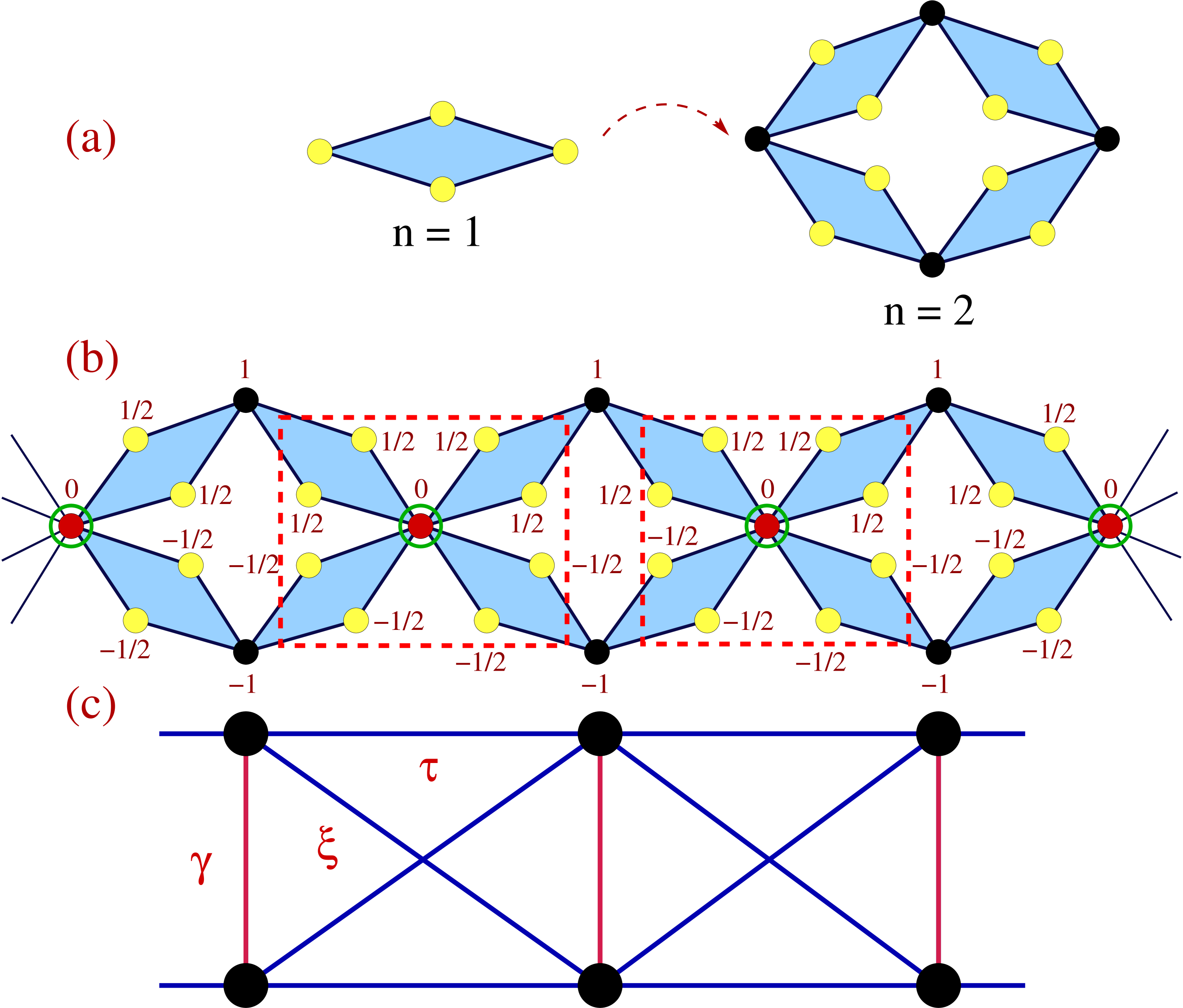
Figure 5: (Color online) (a) Generation and growth of a closed loop Berker-diamond array. (b) Distribution of amplitudes $\psi_{i}$ for a flat band at $E=2$. We have set $t=1$. (c) Conversion of a closed loop Berker-diamond array into a two arm ladder network.

Fig. 5, can be mapped into an effective ladder (drawn by blue lines) by decimating out the vertices trapped inside the red-dashed boxes. There are two kinds of vertices now, viz., with $z=2$ and $z=4$. The on-site potentials bear the symbols $\epsilon_{2}$ and $\epsilon_{4}$ respectively. The FBS are extracted by solving the equation $E-\epsilon_{2,n}=0$. In Fig. 6 we demonstrate the distribution of only the flat band states against varying magnetic flux for open-ended (Fig. 6(a)) and closed-loop (Fig. 6(b)) Berker-diamond arrays. The figure brings out the interesting contrast between the two lattices. The FBS for the

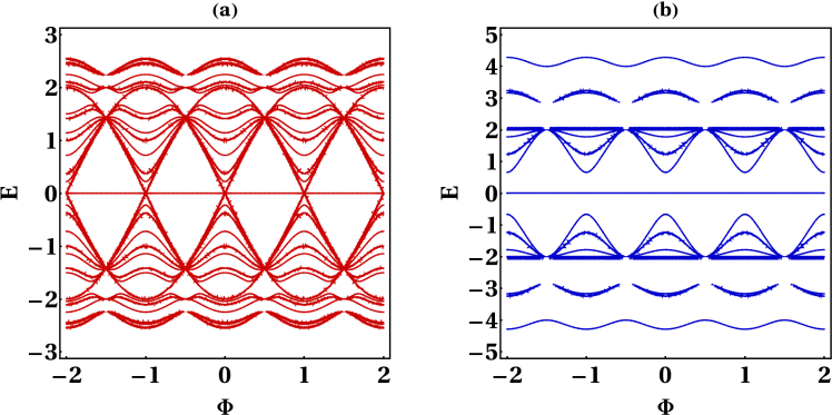
Figure 6: (Color online). Distribution of the flat, non-dispersive states only for (a) an open ended Berker-diamond array in its $3$rd generation, and (b) a closed loop Berker-diamond array in its $3$rd generation. We set $\epsilon_{2}=\epsilon_{4}=0$, $t=1$, and energy is measured in units of $t$.

open ended Berker geometry are grossly divided into two segments above and below the non-dispersive state at $E=0$. The subgroups of such states touch each other at $E=0$, mimicking a Dirac cone. On the other hand the FBS for the closed loop diamond hierarchical array exhibit global gaps along the energy axis as well as for changing values of the magnetic flux. The edge states in both the cases are seen to be most affected by the magnetic field, which is likely to lower the persistent current for such energy regimes.

Before ending this section, it is pertinent to comment that, in all the cases discussed so far, the amplitudes of the FBS are confined within a single unit cell of the lattice under consideration. Such states thus belong to the $U=1$ class of FBS as per the nomenclature introduced by Danieli et al. flach3 . However, the rule of constructing the distribution of amplitudes, as shown as an example in Fig. 4(b) can be implemented for any arbitrarily large generation of the lattice. This is simple, as any large lattice can be renormalized precisely to the one displayed in Fig. 4(b). We need to fix the amplitudes of the flat band wave function to the values $0$, $\pm 1$ and $\pm 1/2$ on the appropriate vertices of the renormalized lattice, exactly in the way depicted in Fig. 6. One can then easily work in the backward direction to extract the distribution in the bare scale of length  atanu .

IV Controlling effective mass with magnetic flux

The analyses presented in the previous sections lead to an interesting prospect. The effective mass of an electron travelling in these kinds of

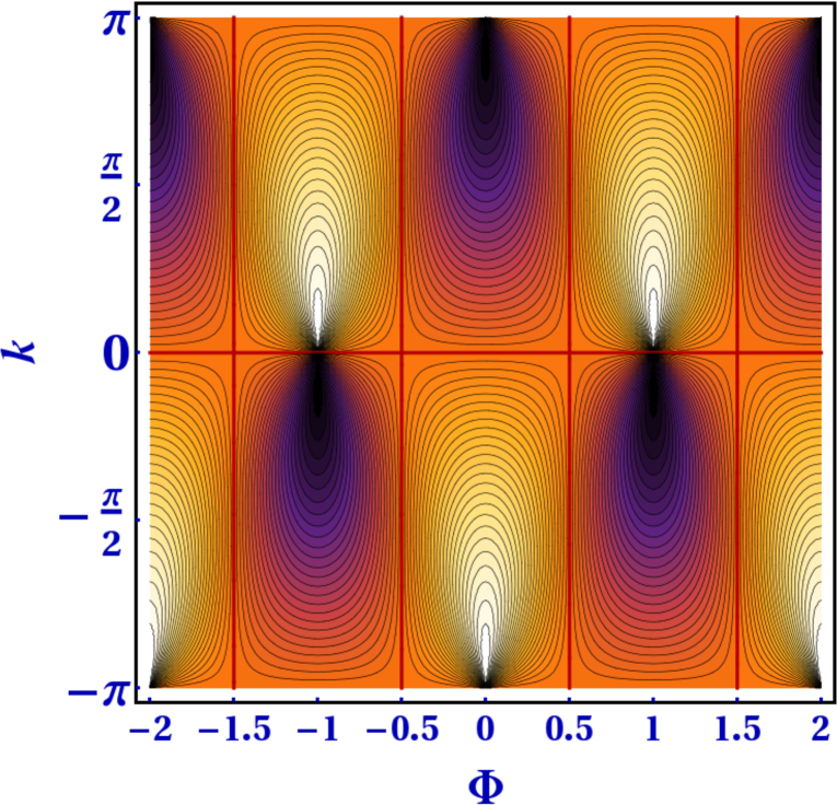
Figure 7: (Color online). Fingerprints of the group velocity of the electron in an elementary diamond array. The sections between the red lines are filled with a continuous distribution of $v_{g}$. We set $\epsilon_{2}=\epsilon_{4}=0$, $t=1$, and display only a few contours to help appreciate the discussion in the text.

arrays can be controlled by tuning the external magnetic field in a non-trivial fashion. This result is a generic feature of an array of diamond network, and is thus common to the Fibonacci-diamond and Berker-diamond class. The microscopic variations are, of course sensitive to the specific aperiodic geometry one introduces along the arm of a diamond. We explain the basics with the help of the simplest model of a diamond array, as depicted in Fig. 1, but now without the diagonal hopping $\tilde{t}$. A uniform magnetic flux $\Phi$ pierces every plaquette. Such a geometry can easily be mapped on to an effectively linear chain, such as depicted in Fig. 1(c). The renormalized on-site potentials and nearest neighbor hopping integrals on this chain, with $\epsilon_{2}=\epsilon_{4}$ are given by,

$$\epsilon^{\prime} = \epsilon+\frac{4t^{2}}{E-\epsilon}$$

$$t^{\prime} = \frac{2t^{2}\cos(\pi\Phi/\Phi_{0})}{E-\epsilon}$$ (27)

The dispersive bands are given by,

$$E=\epsilon\pm 2t\sqrt{1+\cos\left(\frac{\pi\Phi}{\Phi_{0}}\right)\cos(ka)}$$ (28)

Before presenting the variation of the effective mass with flux, it is essential to remind ourselves that, as an electron travels around a trapped magnetic flux, the wave function picks up a phase, viz., $\psi\rightarrow\psi_{0}\exp\left(i\oint\vec{A}.d\vec{l}\right)$, the line integral in the exponent being the flux trapped in the closed loop. The magnetic flux here plays a role equivalent to the wave vector gefen . One can thus conceive of a $k-\Phi$ diagram which is equivalent to a typical $k_{x}-k_{y}$ diagram for electrons travelling in a two dimensional periodic lattice. The “Brillouin zone” equivalents are expected to show up, across which variations of the group velocity and the effective mass will take place.

This is precisely the situation as depicted in Fig. 7. Every contour displayed corresponds to a fixed value of the group velocity which exhibits a period equal to $2\Phi_{0}$. The red lines are the equivalents of the Brillouin zone boundaries across which the group velocity flips its sign if one moves parallel to the $\Phi$-axis at a fixed value of $k$, or vice versa. This implies that, one can, in principle, make an electron retard without changing its energy by tuning the external flux alone. The group velocity is exactly zero along the red lines, showing that the eigenfunctions are self-localized around finite clusters of sites, making the electronic state a non-dispersive, flat one, as we discussed in the beginning.

However, a more serious issue crops up as we note that the same numerical value of the group velocity may lead to a positive, or a negative effective mass of the electron depending on the curvature of the dispersive band at those particular values of the group velocity. This is not apparent from the $k-\Phi$ diagram in Fig. 7, but becomes explicit if we look at the expression of the effective mass which is given by,

$$m^{\ast}=\pm\frac{{\hbar}^{2}}{a^{2}t\left[\frac{\cos(\frac{\pi\Phi}{\Phi_{0}})\cos{ka}}{\sqrt{1+\cos(\frac{\pi\Phi}{\Phi_{0}})\cos{ka}}}+\frac{\cos^{2}(\frac{\pi\Phi}{\Phi_{0}})\sin^{2}(ka)}{2[1+\cos(\frac{\pi\Phi}{\Phi_{0}})\cos(ka)]^{3/2}}\right]}$$ (29)

In Fig. 8 we display the variation of the effective mass against

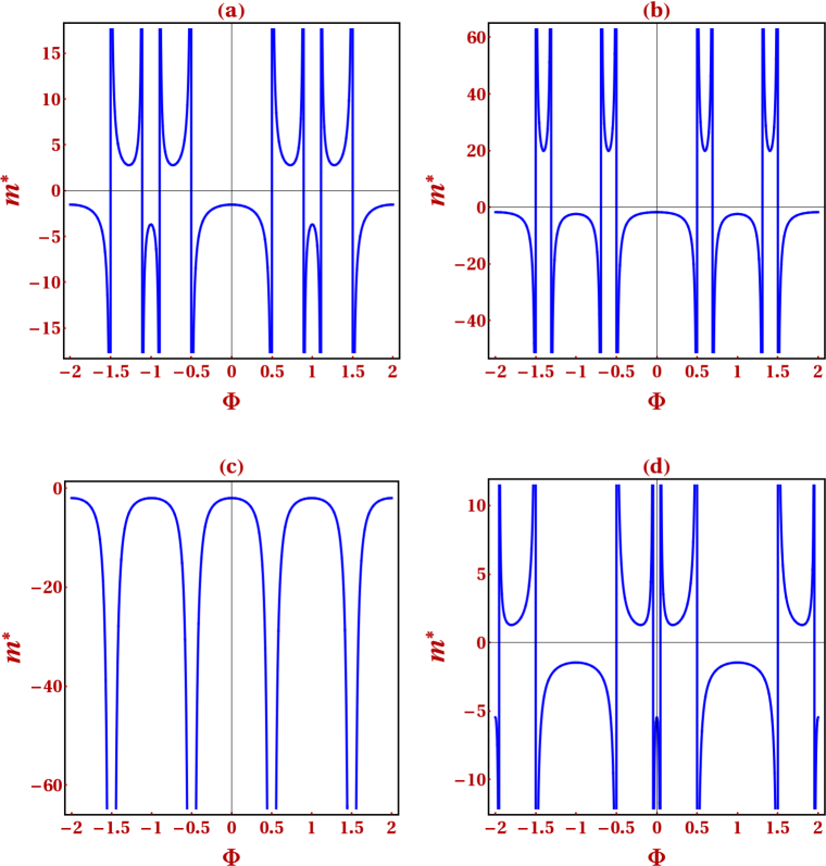
Figure 8: (Color online). Effective mass of an electron traversing a simple diamond array plotted against the magnetic flux at (a) $ka=\pi/4$, (b) $ka=2\pi/5$, (c) $ka=\pi/2$, and (d) $ka=5\pi/6$. We have set $\epsilon=0$ and $t=1$ and energy is measured in unit of $t$.

a changing magnetic field (flux) for different values of the wave vector $k$. For $0<ka<\pi/2$ , the effective mass displays a re-entrant behavior, going from a negative value below $\Phi<\Phi_{0}/2$ to a positive value above the half flux quantum through a divergence shown precisely at the half flux quantum. The exception to this general character takes place at $ka=\pi/2$, which is the first quarter of the band. The effective mass remains negative for all values of the magnetic flux, diverging at $\Phi=(p+1/2)\Phi_{0}$, with $p=0$, $\pm 1$, $\pm 2$, $.......$ The divergences and crossover in the sign of the effective mass are repeated in the interval $1/2\leq\Phi/\Phi_{0}\leq 3/2$. The variation of $m^{\ast}$ is flux periodic with a period equal to $\Phi/\Phi_{0}=2$.

This discussion points to the obvious implication that the electron-lattice interaction can be tuned at will by controlling the magnetic flux from outside. The usual idea that the electron is made to behave like a positively charged particle in a certain part of the band where its effective mass turns negative yields, in this case, a wider variety of phenomenon where this can be achieved in a re-entrant fashion throughout the band, by tuning an external perturbation, that is, the magnetic field. To the best of our knowledge, this simple aspect of such problems was not highlighted before.

V conclusions

We have shown how to extract the eigenvalues corresponding to the localized, non-dispersive, degenerate flat band eigenstates of an infinite, periodic diamond loop array, where aperiodic structures of increasing hierarchy grow on each arm of a basic diamond network. A real space renormalization group scheme is exploited to unravel a countable infinity of such states. The grouping of the dispersive and non-dispersive bands in each case resembles the actual band structure of the quasiperiodic or fractal lattices considered here, as their generation tends to the respective thermodynamic limits. An external magnetic field is shown to be able to control the curvature of the dispersive bands, and hence the sharpness of localization. The group velocity and the effective mass of the electron are thus shown to exhibit a re-entrant behavior inside a single Brillouin zone, a fact that turns out to be a consequence of the quasi-one dimensionality of the loop structure. The scheme is easily extendable to photonic, phononic of magnonic excitations, and the flat band eigenstates for an aperiodically grown superlattice can thus be worked out. This may throw new challenges to experimentalists to engineer the formation and positioning of the non-dispersive energy bands in such artificial lattices. A possible application in device technology may thus be on the cards.

Acknowledgement

Atanu Nandy acknowledges financial support from the UGC, India through a research fellowship [Award letter no. F.$17$-$81/2008$ (SA-I)].

References

- (1) O. Derzhko, J. Richter, and A. Honecker, J. Phys.: Conference Series 145, 012059 (2009).
- (2) J. T. Chalker, T. S. Pickles, and P. Shukla, Phys. Rev. B 82, 104209 (2010).
- (3) A. A. Lopes and R. G. Dias, Phys. Rev. B 84, 085124 (2011).
- (4) A. A. Lopes. B. A. Z. António, and R. G. Dias, Phys. Rev. B 89, 235418 (2014).
- (5) D. Leykam, S. Flach, O. Bahat-Treidel, and A. S. Desyatnikov, Phys. Rev. B 88, 224203 (2013).
- (6) M. Hyrkäs, V. Apaja, and M. Manninen, Phys. Rev. A 87, 023614 (2013).
- (7) S. Flach, D. Leykam, J. D. Bodyfelt, P. Matthies, and A. S. Desyatnikov, Europhys. Lett. 105, 30001 (2014).
- (8) C. Danieli, J. D. Bodyfelt, and S. Flach, arXiv:1502.06690 (2015).
- (9) H. Kikuchi, Y. Fujii, M. Chiba, S. Mitsudo, T. Idehara, T. Tonegawa, K. Okamoto, T. Sakai, T. Kuwai, and H. Ohta, Phys. Rev. Lett. 94, 227201 (2005).
- (10) A. M. S. Macêdo, M. C. dos Santos, M. D. Coutinho-Filho, and C. A. Macêdo, Phys. Rev. Lett. 74, 1851 (1995).
- (11) J. Vidal, R. Mosseri, and B. Douçot, Phys. Rev. Lett. 81, 5888 (1998).
- (12) J. Vidal, B. Douçot, R. Mosseri, and P. Butaud, Phys. Rev. Lett. 85, 3906 (2000).
- (13) J. Vidal, P. Butaud, B. Douçot, and R. Mosseri, Phys. Rev. B 64, 155306 (2001).
- (14) O. Derzhko, J. Richter, A. Honecker, M. Maksymenko, and R. Moessner, Phys. Rev. B 81, 014421 (2010).
- (15) W. Yao, S. A. Yang, and Q. Niu, Phys. Rev. Lett. 102, 096801 (2009).
- (16) I. Bloch, J. Dalibard, and W. Zwerger, Rev. Mod. Phys. 80, 885 (2008).
- (17) D. N. Christodoulides, F. Lederer, and Y. Silberberg, Nature, 424, 817 (2003).
- (18) N. Masumoto, N. Y. Kim, T. Byrnes, K. Kusudo, A. Löffler, S. Höfling, A. Forchel, and Y. Yamamoto, New. J. Phys. 14, 065002 (2012).
- (19) Z. Liu, F. Liu, and Y.-S. Wu, Chin. Phys. B 23, 077308 (2014).
- (20) G.-B. Jo, J. Guzman, C. K. Thomas, P. Hosur, A. Vishwanath, and D. M. Stamper-Kurn, Phys. Rev. Lett. 108, 045305 (2012).
- (21) K. Shiraishi, H. Tamura, and H. Takayanagi, Appl. Phys. Lett. 78, 3702 (2001).
- (22) A. Nandy, B. Pal, and A. Chakrabarti, J. Phys.: Condens. Matt. 27, 125501 (2015).
- (23) M. Kohmoto, B. Sutherland, and C. Tang, Phys. Rev. B 35, 1020 (1987).
- (24) R. Griffiths and M. Kaufman, Phys. Rev. B 26, 5022 (1982).
- (25) S. Sil, S. K. Maiti, and A. Chakrabarti, Phys. Rev. Lett. 101, 076803 (2008).
- (26) The eigenstate at is situated exactly at the edge of a continuous sub-band of the diamond array, as can be easily checked by working out the density of states of this periodic system.
- (27) S. Chattopadhyay and A. Chakrabarti, Phys. Rev. B 65, 184204 (2002).
- (28) H.-F. Cheung, Y. Gefen, E. K. Riedel, and W.-H. Shih, Phys. Rev. B 37, 6050 (1988).