Abstract

The temperature dependence of the topological susceptibility in QCD, $\chi_{t}$, essentially determines the abundance of the QCD axion in the Universe, and is commonly estimated, based on the instanton picture, to be a certain negative power of temperature. While lattice QCD should be able to check this behavior in principle, the temperature range where lattice QCD works is rather limited in practice, because the topological charge is apt to freezes at high temperatures. In this work, two exploratory studies are presented. In the first part, we try to specify the temperature range in the quenched approximation. Since our purpose here is to estimate the range expected in unquenched QCD through quenched simulations, hybrid Monte Carlo (HMC) algorithm is employed instead of heatbath algorithm. We obtain an indication that unquenched calculations of $\chi_{t}$ encounter the serious problem of autocorrelation already at $T\sim 2\,T_{c}$ or even below with the plain HMC. In the second part, we revisit the axion abundance. The absolute value and the temperature dependence of $\chi_{t}$ in real QCD can be significantly different from that in the quenched approximation, and is not well established above the critical temperature. Motivated by this fact and precedent arguments which disagree with the conventional instanton picture, we estimate the axion abundance in an extreme case where $\chi_{t}$ decreases much faster than the conventional power-like behavior. We find a significant enhancement of the axion abundance in such a case.

1 Introduction

It is widely believed that the instanton calculus in QCD [1] makes sense at high temperatures. The asymptotic freedom ensures the perturbative expansion sensible and, most importantly, the infrared divergences from the large instanton contributions are cut-off by the Debye length, providing finite results after the integration over the instanton size [2].

In the semi-classical instanton picture, physics becomes $\theta$-parameter dependent by the instanton contributions to the path integral [3]. The instanton calculus indicates that such a dependence is proportional to the product of the quark masses, $m_{q}^{N_{f}}$ and $\Lambda_{\rm QCD}^{b}$, where $b$ is the beta-function coefficient, $b=11N_{c}/3-2N_{f}/3$. For example, the topological susceptibility, $\chi_{t}=(\partial^{2}/\partial\theta^{2})V_{\rm eff}(\theta)$, is proportional to $m_{q}^{N_{f}}\Lambda_{\rm QCD}^{b}T^{4-N_{f}-b}$ by the dimensional analysis.

In the QCD axion model to solve the strong CP problem, the $\theta$ angle is promoted to the axion field $a(x)/f_{a}$, where $f_{a}$ is the axion decay constant [4, 5, 6, 7, 8, 9, 10, 11]. The topological susceptibility is directly related to the mass of the axion as $\chi_{t}=m_{a}^{2}f_{a}^{2}$. Therefore, the temperature dependence of $\chi_{t}$ discussed above represents that of the axion mass, which is important for the calculation of the axion abundance in the Universe. In the misalignment mechanism for the axion generation in the early Universe, the axion number density is proportional to the axion mass at the temperature at which the axion field starts coherent oscillations [12, 13, 14]. The instanton based estimation of the temperature dependence is commonly used in the literature, and predicts that the axion can naturally be dark matter of the Universe when $m_{a}\sim 10^{-5}$ eV, whereas the astrophysical bound on $m_{a}$ is $m_{a}\lesssim 10^{-2}$ eV. (See, e.g., [15].) The allowed region, $10^{-5}~{}{\rm eV}\lesssim m_{a}\lesssim 10^{-2}~{}{\rm eV}$, is called the “axion window.”

There have been arguments which imply the disappearance of the instanton effects at high temperatures. In Ref. [16], it has been argued in two-flavor QCD that the difference between the two-point functions of iso-singlet and iso-vector scalar operators vanishes in the chiral limit as fast as $O(m_{q}^{2})$ when the temperature is higher than the critical temperature. By the Ward-Takahashi identities, this immediately means that $\chi_{t}$ should be at most an $O(m_{q}^{4})$ quantity, that is different from $O(m_{q}^{2})$ from the instanton calculus. Moreover, in a recent paper [17], it is claimed that $\chi_{t}$ is $O(m_{q}^{N})$ with an arbitrary $N$ and thus it is vanishing even with finite quark masses. Although these are somewhat surprising results, it is certainly possible that the instanton picture fails to describe the full quantum mechanical vacuum [18]. If that is the case, the estimation of the axion abundance is significantly affected.

The lattice simulations can in principle discriminate whether instantons make sense or not. However, the current situation is not conclusive. In Refs. [19, 20], the temperature dependence of various susceptibilities are measured, which seem to be consistent with the semi-classical instanton picture and but at the same time not to exclude other possibilities. Meanwhile, the analysis in Ref. [21] suggests the effective restoration of $U_{A}(1)$ symmetry right above the critical temperature, indicating the disappearance of the instanton effects. The presence or absence of the $U_{A}(1)$ symmetry at the critical temperature $T_{c}$ can also be inferred through the nature of the chiral phase transition of massless two flavor QCD as attempted in, e.g., Ref. [22] (For a related work analyzing the system with the renormalization group flow, see Ref. [23]). See Ref. [24] for a new proposal to extract the instanton effects in lattice QCD, and Ref. [25] for the approach from holography.

One unavoidable problem on the lattice is that the range of the temperature in which one can reliably study the temperature dependence of $\chi_{t}$ is rather limited, because the net susceptibility $\chi_{t}V$, where $V$ is the volume, rapidly decreases with temperature and hence the topology tends to freeze at high temperature. This problem is fatal especially in dynamical lattice QCD simulations since one can not realize arbitrary large volumes while keeping both the light quark masses and lattice artifacts reasonably small. Then, it is natural to ask to what temperature $\chi_{t}$ can be reliably calculated in dynamical QCD with a typical setup. From this viewpoint, determining the precise value of quenched $\chi_{t}(T)$ with large volumes and huge statistics would not provide useful information.

For the reliable calculation of $\chi_{t}$, it is preferable to use lattice chiral fermion for dynamical quarks. But such dynamical simulations at high temperatures are too costly to start with. As the second best, we choose to perform quenched simulations with hybrid Monte Carlo (HMC) algorithm and Iwasaki gauge action. The reasons for these choices are as follows. To answer the above question, the simulation environment needs to be as close to that in dynamical one as possible. Long auto-correlation of the topological charge is one of the serious bottlenecks in dynamical simulations, and the heatbath algorithm, which is available only in the quenched approximation, is faster but has totally different property from HMC in this regard. Iwasaki gauge action is known to result in relatively long autocorrelation time for the topological charge [26, 27]. Thus, we expect that more information about dynamical simulations will be gained from quenched one by taking HMC and Iwasaki gauge action rather than taking heatbath and the standard plaquette gauge action.

Another issue to be addressed is the definition of topological charge $Q$. There is a subtlety in measuring $Q$ if one adopts the field theoretical (or bosonic) definition. This method requires a suitable number of coolings of gauge configurations. If one applies it too much or too less, one would miss the right value of $Q$. Even if one ceases the cooling adequately, $Q$ thus obtained is not an integer, and in the worst case it may be right in the middle of two integers, which can cause misidentification of $Q$. Misidentifications are potentially dangerous, especially at high temperatures (i.e. when $\langle Q^{2}\rangle=\chi_{t}(T)\,V$ is tiny), because it can significantly affect $\chi_{t}(T)$ even if it occurs only rarely. Importantly, it is not possible to know the right value of $Q$ without comparing that obtained with the fermionic definition based on Atiyah-Singer index theorem. From this viewpoint, the use of the fermionic definition has an advantage, although it is much more demanding than the bosonic one. Studying the autocorrelation of $Q$ usually requires high statistics. Thus, this choice of the definition seriously limits the lattice size to small.

In this paper, we first explore to which temperature quenched simulations using HMC and Iwasaki gauge action are able to obtain reliable results for $\chi_{t}$, where the topological charge $Q$ in each configuration is determined by the number of zero modes of overlap Dirac operator. Because of this choice, the lattice volumes are limited to relatively small. Our quenched calculations show that $\chi_{t}$ is undetermined above $T=2\ T_{c}$ for $N_{t}=4$ and $T=1.5\ T_{c}$ for $N_{t}=6$, where $N_{t}$ is the number of lattice sites in the time direction.

This observation suggests two possibilities. One is that the result with $N_{t}=6$ is right and $\chi_{t}$ suddenly decreases at $T\lesssim 1.5\,T_{c}$. In the language of the semi-classical instanton picture, this behavior can happen if there is a sharp short-distance cut-off in the instanton size parameter $\rho$ so that small instantons do not contribute to the path integral. (See [28, 29] for the instanton based models and lattice results suggesting this picture.) If $\chi_{t}$ exhibits such a sharp fall off, the estimation of the abundance of the QCD axion in the Universe may be significantly affected. However, this possibility appears to be unlikely because our value of $\chi_{t}$ with $N_{t}=4$ is reasonably consistent with the previous calculations to $T\sim 1.75\,T_{c}$. Another possibility is that, in the standard HMC with a fixed acceptance ratio, the suppression of $\chi_{t}$ due to the long autocorrelation, which increases with a lattice volume, overcomes the enhancement by enlarging the volume. Through the analysis of the autocorrelation, we confirm the latter to be the case.

Outcome of the first part is that with HMC the reliable calculation of $\chi_{t}$ is difficult for $T\gtrsim 2\,T_{c}$ even in the quenched approximation. Since quenched simulations are always easier than dynamical one, the above outcome or even worse should hold for dynamical QCD.

The second part of the paper goes as follows. We first emphasize that even in the quenched theory it is hard to justify instanton calculus from the first principles because instanton description consists of the perturbative expansion in terms of the strong coupling constant $\alpha_{s}(T)$ and its prediction is only reliable above $T=$ a few GeV. The same is true or the situation is even worse for dynamical QCD. Furthermore, there exist convincing arguments that the presence of light dynamical quarks could drastically change $\chi_{t}$ above $T_{c}$ as stated above. Therefore, not much has been known about the unquenched theory, and there are many degrees of freedom in the choice of $T$ dependence of $\chi_{t}$ above $T_{c}$.

We revisit the axion abundance with some extreme but yet allowed temperature dependence of $\chi_{t}$. We find that the axion abundance is significantly enhanced compared to the conventional estimates with non power-like behavior of $\chi_{t}$ and, for some cases, the axion window is closed depending on how quickly $\chi_{t}$ disappears.

2 Topological susceptibility on the lattice

In the continuum, the topological susceptibility, $\chi_{t}$, is defined as

$$\chi_{t} =\left(1\over 64\pi^{2}\right)^{2}\int d^{4}x\langle\epsilon^{\mu\nu\rho\sigma}F_{\mu\nu}^{a}F_{\rho\sigma}^{a}(x)\epsilon^{\mu^{\prime}\nu^{\prime}\rho^{\prime}\sigma^{\prime}}F_{\mu^{\prime}\nu^{\prime}}^{b}F_{\rho^{\prime}\sigma^{\prime}}^{b}(0)\rangle.$$ (1)

This quantity is related to the axion mass, $m_{a}$, through

$$\chi_{t} =m_{a}^{2}f_{a}^{2},$$ (2)

where $f_{a}$ is the axion decay constant. Through the Atiyah-Singer index theorem, one can also find

$$\chi_{t} ={\langle Q^{2}\rangle\over V},$$ (3)

where the topological charge, $Q=n_{+}-n_{-}$, is the difference between the numbers of the left and the right-handed zero modes in the eigenvectors of the Dirac operator.

On the lattice, the definition of gauge field strength tensor, $F_{\mu\nu}$, is not unique, and so is $\chi_{t}$ if one simply follows Eq. (1). With the definitions of $F_{\mu\nu}$ commonly used in the literature, $Q$ measured by

$$Q =\left(1\over 64\pi^{2}\right)\int d^{4}x\epsilon^{\mu\nu\rho\sigma}F^{a}_{\mu\nu}F^{a}_{\rho\sigma},$$ (4)

takes non-integer values in general. Thus, a technique called “cooling” is usually applied to guess the right integer for $Q$.

Similarly to the continuum, an alternative is to count the zero eigenvalues of the lattice Dirac operator. This requires lattice Dirac operators to satisfy the Ginsparg-Wilson relation [30]. The overlap Dirac operator, $D_{\rm ov}$, is known as such an operator [31], with which one can express $Q$ as

$$Q ={\rm Tr}\Gamma_{5},$$ (5)

where

$$\Gamma_{5} =\gamma_{5}\left(1-{D_{\rm ov}\over 2M_{0}}\right)={1\over 2}\left[{\gamma_{5}}-{\rm sgn}(H_{W}(-M_{0}))\right].$$ (6)

Here, $H_{W}=\gamma_{5}D_{W}(-M_{0})$, and $D_{W}(-M_{0})$ is the Wilson Dirac operator with a negative mass parameter, $-M_{0}$. This definition provides an integer value of $Q$ in each configuration. The trace of the spinor indices of $\Gamma_{5}$, ${\rm tr}\Gamma_{5}$, can provide a definition of the local value of the topological density, $(1/64\pi^{2})\epsilon^{\mu\nu\rho\sigma}F_{\mu\nu}^{a}F_{\rho\sigma}^{a}$.

As stated in the introduction, the bosonic definition has the chance to misidentify $Q$. While, below and around the (pseudo-)critical temperature, previous works have revealed that the bosonic and fermionic definitions of $Q$ give consistent results for $\chi_{t}$, it is not well established above $1.5\,T_{c}$ yet. Especially, we have to keep in mind that a tiny amount of misidentification of $Q$ may bring significant effects to the resulting $\chi_{t}$ at high temperatures as follows.

Whether the instanton picture are correct, it is certainly true that $\chi_{t}$ decreases with the temperature and $\chi_{t}V$ as well. Since $\chi_{t}V$ represents a net width of the fluctuation of $Q$, the fraction of configurations with non-zero $Q$ becomes much smaller than that with the vanishing $Q$ when $\chi_{t}V\ll 1$. Suppose that $N_{\rm conf}$ configurations are generated on the lattice volume of $N_{V}=N_{s}^{3}\times N_{t}$ and that $q$ of them belong to either $Q=+1$ or $Q=-1$ while the others to $Q=0$. This yields $a^{4}\chi_{t}$ = $\langle Q^{2}\rangle/N_{V}$ = $(q+\delta_{\rm mis})/(N_{\rm conf}\ N_{V})$, where $\delta_{\rm mis}/N_{\rm conf}$ represents the rate of misidentification. Then, it should be noted that, even if $\delta_{\rm mis}/N_{\rm conf}$ is tiny, $a^{4}\chi_{t}$ may significantly deviate from a real value because the fraction of nonzero $Q$ configurations, $q/N_{\rm conf}$, is also tiny at high temperatures. To avoid the misidentification, we adopt the fermionic definition in Eq. (5) for the evaluation of $\chi_{t}$.

3 $\chi_{t}(T)$ in the quenched approximation with HMC

3.1 lattice parameters

To calculate the topological susceptibility at finite temperatures, we perform lattice simulations of $SU(3)$ pure Yang-Mills theory around and above $T_{c}$. We employ the Hybrid Monte Carlo (HMC) algorithm to study the autocorrelation of topological charge in HMC for the reason described in introduction. To avoid the ordinary finite size effects, the aspect ratio is set to three or four, which is usually considered to be safe. In addition, we have to recall that the size of fluctuation of $Q$ is directly affected by a volume through $\langle Q^{2}\rangle=\chi_{t}\,V$, which is a finite size effect specific to and important in the calculation of $\chi_{t}$. The calculation is carried out on three lattice volumes using the Iwasaki gauge action, $16^{3}\times 4$, $18^{3}\times 6$ and $24^{3}\times 6$. The topological charge $Q$ is calculated at every ten trajectories. The statistical errors are estimated by the standard jack-knife method with the bin size of 500 trajectories.

The correspondence between $\beta$ and $T/T_{c}$ for the Iwasaki gauge action is read from Ref. [32]. We accumulated 2000 to 40000 trajectories, depending on the simulation parameters, which are summarized in Tab. 1.

$V/a^{4}$	$\beta$	$T/T_{c}$	# of traj.	$\delta\tau$	acc.	$\chi_{t}/T_{c}^{4}$
$16^{3}\times 4$	2.288	1.00	5000	1/55	0.79	0.126(12)
	2.450	1.34	15000	1/60	0.78	0.176(17)$\times 10^{-1}$
	2.522	1.50	19970	1/65	0.78	0.66(9) $\times 10^{-2}$
	2.623	1.75	39860	1/62	0.77	0.43(11) $\times 10^{-2}$
	2.716	2.00	33660	1/67	0.79	0.90(41) $\times 10^{-3}$
	2.802	2.25	43250	1/65	0.79	[0.9(9) $\times 10^{-4}$]
$18^{3}\times 6$	2.445	0.89	4500	1/80	0.82	0.148(18)
	2.515	1.00	19500	1/80	0.82	0.143(14)
	2.710	1.34	17560	1/80	0.80	[0.57(21)$\times 10^{-2}$]
	2.794	1.50	15710	1/80	0.79
	3.018	2.00	17050	1/80	0.78
$24^{3}\times 6$	2.445	0.89	4600	1/77	0.73	0.111(15)
	2.794	1.50	2140	1/100	0.80	[0.28(19) $\times 10^{-2}$]
	3.018	2.00	4030	1/100	0.78

Table 1: Simulation parameters. The trajectory length is always set to one. acc. denotes the acceptance ratio. Topological charge $Q$ is calculated every ten trajectories. The statistical errors are estimated by the jackknife method with the bin size of 500 trajectories. The blank indicates that $\chi_{t}$ can not be calculated due to too rare $Q$ changes.

Lattice volumes chosen in the present work are somewhat smaller than other pure YM calculations. The reason is as follows. In order to reduce the ambiguity associated with the definition of $Q$ as much as possible, we decided to use the fermionic definition for $Q$ to calculate $\chi_{t}$. The purpose of this work is to find the highest temperature to which the reliable extraction of $\chi_{t}$ is feasible in HMC, or in other words, at which temperature the autocorrelation time becomes unreasonably long. Such a study usually requires high statistics. Furthermore the fermionic definition is much more expensive than the bosonic one. Thus this choice of definition constrains lattice volumes to be small.

Here let us mention the difference of this work from Ref. [33], which studies the $T$ dependence of $\chi_{t}$ around the critical temperature, using the fermionic definition for $Q$. Two major differences are in the range of the temperature explored and rigorous application of the overlap Dirac operator. The former is originating from the different motivation. Let us explain more about the latter. In Ref. [33], the identification of $Q$ is made using an approximate solution of the Ginsparg-Wilson equation, while we stick to the exact one. They differ in important way. To check the approximated solutions, in Ref. [33] the chirality of the zeromodes ($\psi_{i}^{{\dagger}}\gamma_{5}\psi_{i}$) is examined, and found that its absolute value ranges from 0.4 to 0.9. With our exact method, it only takes +1 or -1 within a rounding error. Therefore, in Ref. [33], the possibility of the misidentification cannot be excluded thoroughly. Indeed, they observe that 2 to 9 % of configurations are misidentified by comparing their approximated solutions and the exact one below the critical temperature. Importantly, it is not clear how well the method based on the approximation works at higher temperatures. In our calculation, the size of zeromodes and near-zeromodes of Hermitian overlap operator $H_{\rm ov}$ differ by a factor of $O(10^{6})$, and we checked for all zeromodes whether the complex conjugate pair is absent. Thus, no ambiguity exists. While 2 to 9 % of misidentifications will not significantly affect $\chi_{t}$ at low temperatures, it does at high temperatures as $\chi_{t}$ itself is very small there. Note that both of the two differences are essential in the study of axion.

3.2 autocorrelation of $Q$

Figure 1 shows the history of $Q$ at several simulations.

Figure 1: History of topological charge $Q$ above $T_{c}$.

It is seen that, on our smallest lattices, $Q$ changes reasonably frequently below $T\leq 1.75\,T_{c}$. But at $T=2\,T_{c}$, we only observe $Q=-1$ for nonzero $Q$. Further increasing $T$ to $T=2.25\ T_{c}$, non-zero $Q$ was only observed in one configuration in spite of our largest statistics. Thus, $\chi_{t}$ is less reliable at $T\gtrsim 2\,T_{c}$. Another remark, which is not plotted, is that while $|Q|$ fluctuates over the range of $-8$ to $+8$ and $-2$ to $+2$ at $T=T_{c}$ and $1.34\,T_{c}$, respectively, $Q$ only takes a value of $-1$, 0 or $+1$ at $T=1.5\,T_{c}$ and $1.75\,T_{c}$. While this is expected as $\chi_{t}$ decreases, the central values and the statistical errors for those temperatures needs to be checked by comparing other works. (The comparison is made later in Fig. 3.)

It is naively expected that $Q$ fluctuates more frequently at larger lattices. However, the plots in Fig. 1 shows the opposite tendency, which indicates that the suppression of $\chi_{t}$ due to the long autocorrelation in HMC with a fixed acceptance ratio overcomes the enhancement by enlarging the volume for our choice of lattice setup.

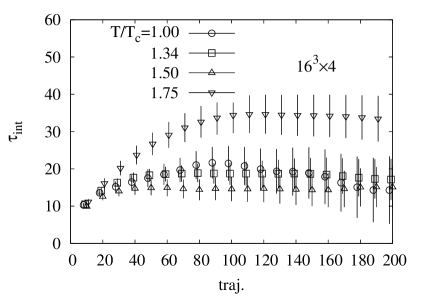
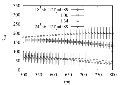
Figure 2: Integrated autocorrelation time for $Q$ on $16^{3}\times 4$ (left) and on the other larger lattices (right).

To quantify the autocorrelation, we estimate the integrated autocorrelation time, $\tau_{\rm int}$. Figure 2 shows that $\tau_{\rm int}$ takes 10 to 20 trajectories at $T\leq 1.5\,T_{c}$ on $16^{3}\times 4$ and increases to about 40 trajectories at $T\leq 1.75\,T_{c}$. Note that we could not obtain $\tau_{\rm int}$ at $T\geq 2.0\,T_{c}$. We observe the qualitatively similar behavior for $18^{3}\times 6$ lattices except for the $T=T_{c}$ data, which shows $\tau_{\rm int}$ larger than other results obtained at $T\sim T_{c}$.

3.3 $T$ dependence of $\chi_{t}$

Figure 3: The temperature dependence of the topological susceptibility, $\chi_{t}$ in unit of $T_{c}^{4}$. The results of $16^{3}\times 4$ (filled circles), $18^{3}\times 6$ (filled squares) and $24^{3}\times 6$ (filled triangles) lattices with the standard HMC are shown. The dotted curve is the fit of five data points of $16^{3}\times 4$ lattices obtained in the range $1\leq T/T_{c}\leq 2$.

The figure 3 shows the $T$ dependence of $\chi_{t}$. It is seen that, restricting the data points to the one in which $Q$ shows a recognizable fluctuation, the results obtained from such fluctuations are consistent with the existing results, for example, given in Ref. [33, 34, 35]. It is important to note that we have only observed $|Q|\leq 1$ at $T=1.50\,T_{c}$ and $1.75\,T_{c}$, but the resulting $\chi_{t}$s nevertheless reasonably agree with the previous results. It is also found that $\chi_{t}$ with different volumes shows consistency within two standard deviations as long as the data showing a recognizable fluctuation of $Q$ are concerned.

To see the consistency of our results with the instanton calculus, we fit the five results in the range of $1\leq T/T_{c}\leq 2$ to the form of $\propto 1/T^{7}$, which is suggested in the leading order instanton calculus. The fit quality is reasonable ($\chi^{2}/$d.o.f.= 0.97).

From these observations, we realized that with HMC it is difficult to obtain the reliable $\chi_{t}$ above $T=2\ T_{c}$ or even $1.5\ T_{c}$ depending on the lattice volume, which immediately indicates the difficulty in dynamical simulations. Even if much faster computers were used, this upper bound will not change significantly. Thus, to estimate the $T$ dependence of $\chi_{t}$ at $O(10\,T_{c})$, we have to make a long extrapolation using those obtained in such a rather limited range of $T$. To push the limit upward as high as possible, it is crucial to explore the HMC parameters or improve the algorithm.

Inspired by Refs. [36, 37], we tried, as an attempt, to enhance the number of configurations with nonzero $Q$ by inserting

$$X=\det\left({H_{W}^{2}+\mu^{2}\over H_{W}^{2}+\epsilon^{2}}\right)^{N_{\phi}},$$ (7)

to the path integral, where $N_{\phi}$ is a positive integer. Then, $\chi_{t}$ is calculated through

$$\chi_{t} ={\langle(Q^{2}/V)XX^{-1}\rangle\over\langle XX^{-1}\rangle}={\langle(Q^{2}/V)X^{-1}\rangle_{X}\over\langle X^{-1}\rangle_{X}},$$ (8)

where $\langle\cdots\rangle_{X}$ denotes the average over the configurations generated with the extra reweighting factor $X$. For $\mu>\epsilon$, the insertion of $X$ enhances the eigenvalue density in the small eigenvalue region, whereas eigenmodes with eigenvalues $\lambda\gg\mu$ are left untouched. Since, when the topology changes, the smallest eigenvalue of $H_{W}$ passes through zero, the above factor is expected to increase such opportunities. However, after we performed some trial calculations, we realized that this method does not always work and the fine tuning of $\mu$, $\epsilon$ and $N_{\phi}$ are required. Further investigations to improve the situation is in progress.

4 Effects of dynamical quarks

Let us discuss what would happen when we include the dynamical quarks. The naive guess would be that $\chi_{t}$ in the Yang-Milles theory is multiplied by a factor of $m_{q}^{N_{f}}/\Lambda_{\rm QCD}^{N_{f}}$ since $\chi_{t}$ should vanish when one of the quark masses goes to zero.

There can be more drastic possibilities. If we accept the claims of the axial $U(1)$ restoration in two-flavor QCD [16, 17], the $O(m_{q}^{2})$ contributions to $\chi_{t}$ is forbidden in two-flavor QCD. Therefore, the possibility of just multiplying by $m_{q}^{N_{f}}/\Lambda_{\rm QCD}^{N_{f}}$ is not consistent. The results of Ref. [17] even forbid contributions with any power of $m_{q}$ for a small $m_{q}$. An extreme possibility one can consider is

$$\chi_{t}(T)\sim\left\{\begin{array}[]{ll}m_{q}\Lambda_{\rm QCD}^{3},&T<T_{c},\\ m_{q}^{2}\Lambda_{\rm QCD}^{2}e^{-2c(m_{q})T^{2}/T_{c}^{2}},&T>T_{c},\\ \end{array}\right.$$ (11)

with $c(m_{q})\to\infty$ as $m_{q}\to 0$, so that $\chi_{t}$ cannot be expanded around $m_{q}=0$. Note that the results of Ref. [17] is contained as a special case of eq. (11). Since no unquenched result of $\chi_{t}$ is available at high temperatures, we take $c(m_{q})$ as a free parameter in the following discussion.

5 Axion abundance

We discuss the impact on the axion abundance in the Universe for the case where the dilute instanton gas approximation fails at high temperatures. One of the source of the axion energy density today is the coherent oscillations of the axion field started in the early Universe. The equation of motion for the axion field, $a$, is given by

$${\ddot{a}}+3H\dot{a}=-m_{a}^{2}(T)a,$$ (12)

where $H$ is the Hubble parameter and $m_{a}(T)$ is the axion mass at a temperature $T$. The axion mass is related to $\chi_{t}$ as in Eq. (2). This equation of motion leads to an oscillating solution. Although the axion mass is temperature dependent, and thus time dependent, the axion number density divided by $T^{3}$, $n_{a}/T^{3}$, stays constant during the oscillation and its value is given by

$${n_{a}\over T^{3}} \simeq{m_{a}(T_{*})f_{a}^{2}\theta^{2}\over T_{*}^{3}},$$ (13)

where $T_{*}$ is the temperature at which the axion field starts to oscillate, and $\theta$ is the initial amplitude of $a/f_{a}$. In the conventional estimates, one uses $m_{a}(T)\propto T^{-4}$ derived by the instanton gas approximation. The temperature $T_{*}$ is obtained by equating $m_{a}(T)$ and the Hubble parameter, $H(T)\sim T^{2}/M_{\rm Pl}$, with $M_{\rm Pl}$ being the Planck scale, such as

$$T_{*} \simeq 1~{}{\rm GeV}\cdot\left(m_{a}\over 10^{-5}~{}{\rm eV}\right)^{1/6}.$$ (14)

By using this value and setting $m_{a}(T_{*})\simeq 3H(T_{*})$, the energy fraction today is finally given by

$$\Omega_{a}\simeq 0.2\cdot\theta^{2}\cdot\left(m_{a}\over 10^{-5}~{}{\rm eV}\right)^{-7/6},$$ (15)

for $\theta\ll 1$, and it is about a factor of two larger for $\theta\sim O(1)$ [38, 39]. According to this formula, the axion can naturally be the dark matter of the Universe for $m_{a}\sim 10^{-5}$ eV which corresponds to $f_{a}=6\times 10^{11}$ GeV. (See Ref. [40] for a recent detailed calculation.)

If the axion mass $m_{a}(T)$ decreases much faster as discussed in the previous section, the axion starts to oscillate near the critical temperature $T_{c}\sim 150$ MeV independent of the axion mass. More importantly, the axion number density gets fixed when the time scale of the oscillation, $1/m_{a}(T)$, is comparable to that of the change of the axion mass, $(\dot{m}_{a}(T)/m_{a}(T))^{-1}$, so that the change of the mass is adiabatic, i.e.,

$$m_{a}(T) \gtrsim\left|{1\over m_{a}(T)}{dm_{a}(T)\over dt}\right|=H(T)\left|{d\ln m_{a}(T)\over d\ln T}\right|.$$ (16)

The condition is automatically satisfied when $m_{a}(T)\sim H(T)$ and $m_{a}(T)\propto T^{n}$ with $n\sim O(1)$, but not necessarily true for exponential functions.

In the model discussed in the previous section, $m_{a}(T)$ is given by

$$m_{a}(T)=m_{a}(T_{c})e^{-c(T^{2}-T_{c}^{2})/T_{c}^{2}},$$ (17)

where the $c$ parameter may be much larger than $O(1)$. The oscillation starts when both sides of Eq. (16) become comparable, and thus

$$m_{a}(T_{*})\sim 2cH(T_{*})\left({T_{*}\over T_{c}}\right)^{2}.$$ (18)

Since $m_{a}(T)$ is a steeply varying function, we expect $T_{*}\sim T_{1}$, where $T_{1}$ is defined by

$$m_{a}(T_{1})=3H(T_{1}).$$ (19)

This causes an enhancement of the axion density by a factor of about $c(T_{1}/T_{c})^{2}$ compared to the conventional estimate in addition to the enhancement due to the shift of the oscillation temperature.

A numerical solution of the equation of motion in Eq. (12) shows that the axion number density is approximately given by

$${n_{a}(T)\over T^{3}}\simeq{0.5c\times 3H(T_{1})f_{a}^{2}\theta^{2}\over T_{1}^{3}}\cdot{T_{1}^{2}\over T_{c}^{2}}={0.5c\times 3H(T_{c})f_{a}^{2}\theta^{2}\over T_{c}^{3}}\cdot{T_{1}\over T_{c}}.$$ (20)

Here

$$T_{1}\sim T_{c}\left[1+{1\over c}\left(12+\log\left(m_{a}(T_{c})\over 10^{-5}~{}{\rm eV}\right)\right)\right]^{1/2}.$$ (21)

Here we used $3H(T_{c})\simeq 5\times 10^{-20}$ GeV, and assumed $(T_{1}/T_{c})^{2}\ll m_{a}(T_{c})/3H(T_{c})$. Putting it all together, the axion energy density today is given by

$$\Omega_{a} \sim 0.2\cdot\theta^{2}\cdot\left({m_{a}\over 10^{-5}~{}{\rm eV}}\right)^{-1}\times 2.5c\left[1+{1\over c}\left(12+\log\left(m_{a}(T_{c})\over 10^{-5}~{}{\rm eV}\right)\right)\right]^{1/2}.$$ (22)

Even for $c=O(1)$ and $m_{a}=10^{-5}$ eV, we find that the axion energy density is enhanced by an order of magnitude compared to the conventional estimate. The enhancement is larger for larger $c$. The axion window is closed when $c\sim 400$. For an extremely large value of $c$, i.e., $c\gtrsim 4\times 10^{5}\cdot(m_{a}/10^{-5}~{}{\rm eV})$, the axion starts to oscillate at $T=T_{c}$. In that case, $\Omega_{a}\sim 2\times 10^{5}\cdot\theta^{2}$ independent of $c$.

We have also examined the case of $\chi_{t}\propto\exp(-2c\,T/T_{c})$ rather than $\chi_{t}\propto\exp(-2c\,T^{2}/T_{c}^{2})$ in Eq. (11). We find a similar enhancement factor $1.0\,c$ instead of $2.5\,c$ in Eq. (22).

In the scenario where the Peccei-Quinn symmetry breaking takes place after the inflation, one should take an average value of $\theta$, $\langle\theta^{2}\rangle\simeq\pi^{2}$. Also, in addition to the misalignment mechanism considered above, there are contributions to the axion density from the axionic strings and domain walls [41, 42, 43, 44]. Both contributions receive an enhancement due to the delay of time scale of the axion production which leads a milder dilution due to the cosmic expansion. The enhancement factor of $\Omega_{a}$ compared to the estimates based on $m_{a}(T)\propto T^{-4}$, $\Omega_{a}^{\rm conv.}$, is the ratio of the temperature in Eq. (14) and the temperature $T_{1}$ at which the adiabatic condition is satisfied. The enhancement factor is

$$\Omega_{a}/\Omega_{a}^{\rm conv.}\Bigg{|}_{\rm string+wall}\simeq 6.6\times\left({m_{a}\over 10^{-5}~{}{\rm eV}}\right)^{1/6}\left[1+{1\over c}\left(12+\log\left(m_{a}(T_{c})\over 10^{-5}~{}{\rm eV}\right)\right)\right]^{-1/2},$$ (23)

For $m_{a}=10^{-5}$ eV, for example, the enhancement is a factor of a few for $c=O(1)$. The value of $\Omega_{a}^{\rm conv.}|_{\rm string+wall}$ is found in Ref. [45]:

$$\Omega_{a}^{\rm conv.}\Big{|}_{\rm string+wall}\sim 4\times\left(m_{a}\over 10^{-5}~{}{\rm eV}\right)^{-7/6}.$$ (24)

6 Summary

The temperature dependence of the topological susceptibility $\chi_{t}$ essentially determines the abundance of the QCD axion in the Universe, and can be calculated using lattice QCD in model independent way. However, at high temperatures, the lattice calculation suffers from various difficulties such as the numerically demanding definition, possible misidentifications and the long autocorrelation of the topological charge.

As the first step towards the precise calculation, we have performed the lattice calculation of $\chi_{t}$ in the $SU(3)$ Yang-Milles theory, focusing on the autocorrelation time in HMC, and found that the problem starts to show up around $T\sim 2.0\,T_{c}$, This immediately indicates the difficulty in dynamical simulations at the similar temperature while estimating the axion abundance in the conventional scenario requires the $T$ dependence up to $O(10\,T_{c})$. To fill this gap, we need exploratory studies of HMC parameters or even algorithm itself.

Meanwhile, in order to see the importance of understanding the temperature dependence of $\chi_{t}$ for the axion abundance in the Universe, we have calculated the axion energy density, $\Omega_{a}$, in an extreme case where $\chi_{t}$ drops exponentially above the critical temperature. It is found that the non-adiabatic growth of the axion potential makes the axion abundance significantly larger, possibly closing the axion window. In this particular case, the behavior of $\chi_{t}$ around $T_{c}$ becomes important.

Our findings provides strong motivation to further serious studies of topology on the lattice and instanton at medium temperatures.

Note added

While this paper was being completed, Ref. [46] appeared which estimates $\chi_{t}$ at high temperatures in the quenched approximation with the heatbath algorithm on large volumes and uses it to discuss the axion abundance. It turns out that our results at $N_{t}=4$ are consistent with theirs to $T\sim 2\,T_{c}$, which give us a more confidence that the autocorrelation time of topological charge increases with volume in HMC and hence increasing volume does not resolve the problem.

References

- [1] G. ’t Hooft, Phys. Rev. D 14, 3432 (1976) [Phys. Rev. D 18, 2199 (1978)].
- [2] R. D. Pisarski and L. G. Yaffe, Phys. Lett. B 97, 110 (1980).
- [3] C. G. Callan, Jr., R. F. Dashen and D. J. Gross, Phys. Rev. D 17, 2717 (1978).
- [4] R. D. Peccei and H. R. Quinn, Phys. Rev. Lett. 38, 1440 (1977).
- [5] R. D. Peccei and H. R. Quinn, Phys. Rev. D 16, 1791 (1977).
- [6] S. Weinberg, Phys. Rev. Lett. 40, 223 (1978).
- [7] F. Wilczek, Phys. Rev. Lett. 49, 1549 (1982).
- [8] J. E. Kim, Phys. Rev. Lett. 43, 103 (1979).
- [9] M. A. Shifman, A. I. Vainshtein and V. I. Zakharov, Nucl. Phys. B 166, 493 (1980).
- [10] M. Dine, W. Fischler and M. Srednicki, Phys. Lett. B 104, 199 (1981).
- [11] A. R. Zhitnitsky, Sov. J. Nucl. Phys. 31, 260 (1980) [Yad. Fiz. 31, 497 (1980)].
- [12] J. Preskill, M. B. Wise and F. Wilczek, Phys. Lett. B 120, 127 (1983).
- [13] L. F. Abbott and P. Sikivie, Phys. Lett. B 120, 133 (1983).
- [14] M. Dine and W. Fischler, Phys. Lett. B 120, 137 (1983).
- [15] J. Engel, D. Seckel and A. C. Hayes, Phys. Rev. Lett. 65, 960 (1990).
- [16] T. D. Cohen, Phys. Rev. D 54, 1867 (1996) [hep-ph/9601216].
- [17] S. Aoki, H. Fukaya and Y. Taniguchi, Phys. Rev. D 86, 114512 (2012) [arXiv:1209.2061 [hep-lat]].
- [18] E. Witten, Nucl. Phys. B 149, 285 (1979).
- [19] M. I. Buchoff, M. Cheng, N. H. Christ, H.-T. Ding, C. Jung, F. Karsch, Z. Lin and R. D. Mawhinney et al., Phys. Rev. D 89, no. 5, 054514 (2014) [arXiv:1309.4149 [hep-lat]].
- [20] T. Bhattacharya, M. I. Buchoff, N. H. Christ, H.-T. Ding, R. Gupta, C. Jung, F. Karsch and Z. Lin et al., Phys. Rev. Lett. 113, 082001 (2014) [arXiv:1402.5175 [hep-lat]].
- [21] G. Cossu, S. Aoki, H. Fukaya, S. Hashimoto, T. Kaneko, H. Matsufuru and J. I. Noaki, Phys. Rev. D 87, no. 11, 114514 (2013) [Phys. Rev. D 88, no. 1, 019901 (2013)] [arXiv:1304.6145 [hep-lat]].
- [22] S. Ejiri and N. Yamada, Phys. Rev. Lett. 110, no. 17, 172001 (2013) [arXiv:1212.5899 [hep-lat]].
- [23] T. Sato and N. Yamada, Phys. Rev. D 91, no. 3, 034025 (2015) [arXiv:1412.8026 [hep-lat]].
- [24] M. Dine, P. Draper and G. Festuccia, arXiv:1410.8505 [hep-ph].
- [25] M. Hanada, Y. Matsuo and T. Morita, Nucl. Phys. B 899, 631 (2015) [arXiv:1505.04498 [hep-th]].
- [26] T. A. DeGrand, A. Hasenfratz and T. G. Kovacs, Phys. Rev. D 67, 054501 (2003) [hep-lat/0211006].
- [27] D. J. Antonio et al. [RBC and UKQCD Collaborations], Phys. Rev. D 75, 114501 (2007) [hep-lat/0612005].
- [28] T. Schëfr and E. V. Shuryak, Rev. Mod. Phys. 70, 323 (1998) [hep-ph/9610451].
- [29] M. C. Chu and S. Schramm, Phys. Rev. D 51, 4580 (1995) [nucl-th/9412016].
- [30] P. H. Ginsparg and K. G. Wilson, Phys. Rev. D 25, 2649 (1982).
- [31] H. Neuberger, Phys. Lett. B 427, 353 (1998) [hep-lat/9801031].
- [32] M. Okamoto et al. [CP-PACS Collaboration], Phys. Rev. D 60, 094510 (1999) [hep-lat/9905005].
- [33] C. Gattringer, R. Hoffmann and S. Schaefer, Phys. Lett. B 535, 358 (2002) [hep-lat/0203013].
- [34] B. Alles, M. D’Elia and A. Di Giacomo, Nucl. Phys. B 494, 281 (1997) [Nucl. Phys. B 679, 397 (2004)] [hep-lat/9605013].
- [35] V. G. Bornyakov, E.-M. Ilgenfritz, B. V. Martemyanov, V. K. Mitrjushkin and M. Müller-Preussker, Phys. Rev. D 87, no. 11, 114508 (2013) [arXiv:1304.0935 [hep-lat]].
- [36] H. Fukaya et al. [JLQCD Collaboration], Phys. Rev. D 74, 094505 (2006) [hep-lat/0607020].
- [37] G. McGlynn and R. D. Mawhinney, PoS Lattice 2013, 027 (2014) [arXiv:1311.3695 [hep-lat]].
- [38] M. S. Turner, Phys. Rev. D 33, 889 (1986).
- [39] D. H. Lyth, Phys. Rev. D 45, 3394 (1992).
- [40] O. Wantz and E. P. S. Shellard, Phys. Rev. D 82, 123508 (2010) [arXiv:0910.1066 [astro-ph.CO]].
- [41] R. L. Davis, Phys. Lett. B 180, 225 (1986).
- [42] R. L. Davis and E. P. S. Shellard, Nucl. Phys. B 324, 167 (1989).
- [43] P. Sikivie [ADMX Collaboration], Phys. Rev. Lett. 48, 1156 (1982).
- [44] D. H. Lyth, Phys. Lett. B 275, 279 (1992).
- [45] M. Kawasaki, K. Saikawa and T. Sekiguchi, Phys. Rev. D 91, no. 6, 065014 (2015) [arXiv:1412.0789 [hep-ph]].
- [46] E. Berkowitz, M. I. Buchoff and E. Rinaldi, arXiv:1505.07455 [hep-ph].