Second-order response theory of radio-frequency spectroscopy for cold atoms

Abstract

We present a theoretical description of the radio-frequency (rf) spectroscopy of fermionic atomic gases, based on the second-order response theory at finite temperature. This approach takes into account the energy resolution due to the envelope of the rf pulse. For a noninteracting final state, the momentum- and energy-resolved rf intensity depends on the fermion spectral function and pulse envelope. The contributions due to interactions in the final state can be classified by means of diagrams. Using this formalism, as well as the local density approximation in two and three dimensions, we study the interplay of inhomogeneities and Hartree energy in forming the line shape of the rf signal. We show that the effects of inhomogeneities can be minimized by taking advantage of interactions in the final state, and we discuss the most relevant final-state effects at low temperature and density, in particular the effect of a finite lifetime.

I Introduction

In many-fermion systems, the low-energy properties are often determined by single-particle excitations across the Fermi surface. The character of these excitations depends on the nature of the ground state, which itself depends on the interactions. The study of single-particle excitations is therefore a key to understanding the ground state and the role of interactions. In superconductors, for instance, a gap in the single-particle excitation spectrum reveals the condensation of Cooper pairs in the ground state. In a large class of materials, the interactions bring only quantitative changes with respect to a noninteracting ground state. The single-particle excitations are then similar to uncorrelated particles, albeit with a renormalized mass and a finite lifetime. The collection of these “quasiparticles” forms a Fermi liquid, which can be characterized by a small number of effective parameters *[][[Sov.Phys.JETP3; 920(1957)].]Landau-1956. For strong interactions and/or reduced dimensionality, qualitative changes may occur in the ground state, leading to the disappearance of the quasiparticles and the emergence of more complex, sometimes mysterious, excitations Stewart (2001); Schofield (1999). The absence of quasiparticles in a fermion system is a hallmark of non-Fermi liquid physics, indicating an unconventional ground state.

For electronic materials, angle-resolved photoemission spectroscopy (ARPES) gives access to the single-particle excitations and allows one to probe the existence of quasiparticles Damascelli et al. (2003). The signature of quasiparticles is a peak at low energy in the spectral function, which is the momentum-energy distribution of the single-particle excitations, denoted $A(\bm{k},\varepsilon)$. Conversely, a structureless spectral function signals the absence of quasiparticles. ARPES experiments require clean surfaces and ultrahigh vacuum, and an energy resolution below the typical excitation energy of the quasiparticles. Steady improvements in recent years and the development of laser ARPES have made it possible to measure the spectral function with excellent resolution in several condensed-matter systems Vishik et al. (2010); Lu et al. (2012); Allan et al. (2013). When it is present, the quasiparticle peak and its dispersion anomalies can help in identifying the interactions that determine the quasiparticle dynamics.

Fermionic cold-atom gases open new avenues in the study of quasiparticles, especially thanks to the possibility of tuning both the dimensionality and the strength of interactions. Radio-frequency (rf) spectroscopy is presently the best method to measure the spectral function of cold-atom systems. Unlike in conventional ARPES, photoemission spectroscopy in ultracold atoms is performed using rf photons, which carry negligible momentum but only supply an energy $h\nu$. The momentum of the extracted atoms is then measured using the time-of-flight technique. If the particles are decoupled in the final state, their energy and momentum distributions follow the spectral function of the photon-induced hole, which is the occupied part of the spectral function, i.e., $A(\bm{k},\varepsilon)f(\varepsilon)$, where $f(\varepsilon)$ is the Fermi function Törmä and Zoller (2000); Dao et al. (2007); *Dao-2009.

The interpretation of photoemission and rf experiments may be complicated by the unavoidable interaction in the final state, as well as several other difficulties. In ARPES, these are, for instance, the sample surface, which breaks inversion symmetry and produces interference, or the screening of the electromagnetic field, which prevents light from entering the bulk of the material. In rf spectroscopy of cold atoms, the main concern is the inhomogeneity of harmonically trapped gases. When interactions and excitation energies are not too low, as in the studies of the BCS-BEC crossover Ketterle and Zwierlein (2008), some of these difficulties may turn out to be irrelevant. For weak interactions, however, they will eventually become important. If the signal is broadened by final-state effects, averaging over inhomogeneities, and finite energy resolution, a precise modeling is necessary in order to recover the crucial information about the quasiparticles.

In the established theory of rf spectroscopy, one computes the instantaneous transition rate to the final state. This can be done either by linear response Törmä and Zoller (2000), which provides the current $\dot{N}_{f}$ of particles transferred to the final state, or by time-dependent perturbation theory (Fermi golden rule) Dao et al. (2007); *Dao-2009. At leading order, $\dot{N}_{f}$ is related to a response function, which can be represented by bubblelike Feynman diagrams Perali et al. (2008). In this approach, the effect of inhomogeneities has been investigated at the mean-field level Ohashi and Griffin (2005) or using the local-density approximation (LDA) He et al. (2005); Dao et al. (2007); *Dao-2009. To circumvent the difficulties raised by inhomogeneity, a Raman local spectroscopy was proposed theoretically Dao et al. (2007); *Dao-2009, while a tomographic technique Shin et al. (2007) and a method to selectively address the cloud center Drake et al. (2012); *Sagi-2012 were demonstrated. Final-state effects have been treated in the mean-field approximation Yu and Baym (2006) by sum-rule arguments Baym et al. (2007); Punk and Zwerger (2007), within a reduced basis Basu and Mueller (2008), a $1/N$ expansion Veillette et al. (2008), diagrammatically Perali et al. (2008); Pieri et al. (2009), or through self-consistency requirements He et al. (2009). Most of these studies have focussed on the BCS-BEC crossover problem.

For intermediate or weak interactions, the finite energy resolution must be considered. The relevant quantity to calculate is no longer $\dot{N}_{f}$, but the total population $N_{f}$ of the final state, created over the duration of the rf pulse. Momentum-resolved rf experiments indeed measure the momentum distribution $n_{f}(\bm{k},t)$ at a time $t$ after the extinction of the rf pulse. If atoms were excited at a constant rate, $\dot{N}_{f}$ and $N_{f}$ would carry the same information, but this is not the case in practice. In this paper, we present the calculation of $n_{f}(\bm{k},t)$ within equilibrium response theory. The derivation is performed in the finite-temperature Matsubara framework. Unlike $\dot{N}_{f}$, $n_{f}$ vanishes at first order in the atom-light coupling. At second order, the momentum distribution is related to a three-point response function, whose contributions can be classified using Feynman diagrams. These diagrams have three external vertices, unlike the bubble diagrams of the established theory, which have only two. The leading contribution reproduces the known result Törmä and Zoller (2000); Dao et al. (2007); *Dao-2009, albeit convolved with a resolution function, which depends on the envelope of the rf pulse and on the spectral function in the final state.

Simulations based on this formalism have been presented earlier Fröhlich et al. (2012) and compared with measurements for ⁴⁰K atoms in two-dimensional harmonic traps with a weak attractive interaction. In this work, it was shown that inhomogeneities must be considered for a correct determination of the quasiparticle effective mass. Here we discuss the role of inhomogeneities in this experiment in more detail and propose ways to reduce their effect. We also show that, in the experiments of Ref. Gupta et al., 2003 made with ⁶Li atoms in three-dimensional harmonic traps, the inhomogeneity sets the line shape of the integrated rf intensity and should be considered for the precise experimental determination of the scattering length.

The paper is organized as follows. In Sec. II.1, we present the model and the calculation of $n_{f}(\bm{k},t)$. The generic diagrams giving the momentum distribution are shown in Sec. II.2, and the leading contribution is evaluated in Sec. II.3. Without interaction in the final state, the analysis simplifies as shown in Sec. III, where we discuss the interplay between the inhomogeneity and the Hartree shifts. We study final-state effects in Sec. IV: the effect of a finite lifetime, the effect of inhomogeneous Hartree shifts, and other final-state effects which correspond diagrammatically to vertex corrections. Conclusions and perspectives are given in Sec. V.

II Finite-temperature, second-order response theory for the momentum distribution

II.1 Description of the model

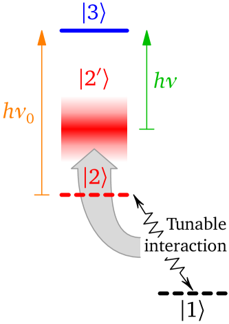
Figure 1: (Color online) Rf spectroscopy of ultracold atoms. The hyperfine atomic levels $|1\rangle$, $|2\rangle$, and $|3\rangle$ are split by the Zeeman effect, such that a rf transition is allowed between states $|2\rangle$ and $|3\rangle$. The tunable many-body interaction between atoms of the cloud in states $|1\rangle$ and $|2\rangle$ shifts and broadens the level $|2\rangle$. The effects of this interaction are probed by comparing the frequency $\nu$ of the rf transition with the frequency $\nu_{0}$ of the noninteracting transition. Spin relaxation from $|2\rangle$ to $|1\rangle$ is forbidden by conservation of spin, meaning that the energy splitting between $|1\rangle$ and $|2\rangle$ is irrelevant. Levels $|1\rangle$ and $|3\rangle$ may be renormalized by interactions as well.

The atoms are modeled as three-level systems with internal states $|\alpha\rangle$, $\alpha=1,2,3$. States $|1\rangle$ and $|2\rangle$ are assumed to interact most strongly, while state $|3\rangle$ has higher energy and will be the final state of the rf experiment; see Fig. 1. We consider that the three levels have the same dispersion; our results are readily generalized to the case where the dispersions are different in the initial and final states. These levels correspond, in practice, to atomic hyperfine states. The interaction between $|1\rangle$ and $|2\rangle$ is resonant and can be tuned by means of a Feshbach resonance Chin et al. (2010). Once the field is set, the interactions between $|1\rangle$ and $|3\rangle$ and between $|2\rangle$ and $|3\rangle$ are also set. Ideally, the latter interactions are small compared with the former. We consider hereafter fermionic atoms, and we assume translation invariance for simplicity. The extension to bosons is straightforward, and the formalism can be developed in real space if needed. Let $c^{\dagger}_{\alpha\bm{k}}$ be the creation operator for an atom in the state $|\alpha\rangle$ with momentum $\hbar\bm{k}$. The low-energy effective Hamiltonian is $H=H_{0}+V$, with

$$H_{0} =\sum_{\bm{k}}\left[\varepsilon_{\bm{k}}(c^{\dagger}_{1\bm{k}}c^{\phantom{\dagger}}_{1\bm{k}}+c^{\dagger}_{2\bm{k}}c^{\phantom{\dagger}}_{2\bm{k}})+(\varepsilon_{\bm{k}}+h\nu_{0})c^{\dagger}_{3\bm{k}}c^{\phantom{\dagger}}_{3\bm{k}}\right]$$ (1)

$$V =\frac{1}{2}\sum_{\stackrel{{\scriptstyle\scriptstyle\bm{k}\bm{k}^{\prime}\bm{q}}}{{\alpha\beta}}}V_{\alpha\beta}(\bm{q})c^{\dagger}_{\alpha\bm{k}}c^{\dagger}_{\beta\bm{q}-\bm{k}}c^{\phantom{\dagger}}_{\alpha\bm{k}^{\prime}}c^{\phantom{\dagger}}_{\beta\bm{q}-\bm{k}^{\prime}}.$$ (2)

We consider here the case of a local interaction between two atoms with center-of-mass momentum $\bm{q}$. The detailed form of the interaction plays no role in our derivation, which is also valid for more general momentum-dependent interactions. For a contact interaction, the Pauli principle prevents atoms in the same internal state from interacting, and we can set $V_{\alpha\alpha}=0$.

The level separation $\nu_{0}$ is typically in the 100 MHz range, and the rf radiation at this frequency has a wavelength of the order of meters. The rf pulse therefore induces momentum-conserving transitions. Let $H^{\prime}(t)$ be the time-dependent interaction between the rf radiation and the atoms, and let us assume that the allowed transition is between states $|2\rangle$ and $|3\rangle$. We have

$$H^{\prime}(t)=\mathcal{E}(t)\sum_{\bm{k}}\left(c^{\dagger}_{3\bm{k}}c^{\phantom{\dagger}}_{2\bm{k}}+\text{h.c.}\right)=\mathcal{E}(t)\sum_{\bm{k}}\gamma^{\phantom{\dagger}}_{\bm{k}}.$$ (3)

The function $\mathcal{E}(t)$ gives the time envelope and strength of the coupling. For later convenience, we define the operator

$$\gamma^{\phantom{\dagger}}_{\bm{k}}=\gamma^{\dagger}_{\bm{k}}=c^{\dagger}_{3\bm{k}}c^{\phantom{\dagger}}_{2\bm{k}}+\text{h.c.}$$ (4)

II.2 Generic diagrams for the momentum distribution

We now expand the momentum distribution in the final state, $n_{\bm{k}}\equiv c^{\dagger}_{3\bm{k}}c^{\phantom{\dagger}}_{3\bm{k}}$, in powers of $H^{\prime}$. In the grand-canonical ensemble, and in the interaction picture, we have

$$\langle n_{\bm{k}}(t)\rangle=\text{Tr}\,\rho n_{\bm{k}}(t),$$ (5)

with $\rho=e^{-\beta(H-\mu N)}/\text{Tr}\,e^{-\beta(H-\mu N)}$, $\beta=1/(k_{\text{B}}T)$, $\mu$ the chemical potential, and $N$ the number operator. Since we work in equilibrium, the chemical potential $\mu$ sets the populations of the three levels, and $N$ is the total atom number. The evolution is given by $n_{\bm{k}}(t)=U^{-1}(t)n_{\bm{k}}U(t)$ with $U(t)$ the interaction part of the evolution operator. The zeroth-order term is obviously

$$\langle n_{\bm{k}}(t)\rangle^{(0)}=\text{Tr}\,\rho n_{\bm{k}}\equiv\langle n_{\bm{k}}\rangle_{H},$$ (6)

which gives the equilibrium thermal population of the final state. For a noninteracting system, this becomes

$$\langle n_{\bm{k}}\rangle_{H_{0}}=f(\varepsilon_{\bm{k}}+h\nu_{0}-\mu),$$ (7)

where $f(\varepsilon)=(e^{\beta\varepsilon}+1)^{-1}$ is the Fermi distribution function. The usual setup is that the final state is initially empty, such that this contribution is negligible at low temperatures, $k_{\text{B}}T\ll h\nu_{0}$. The first-order term in $H^{\prime}$ is known, from standard linear-response theory, to be

$$\langle n_{\bm{k}}(t)\rangle^{(1)} =-\frac{i}{\hbar}\int_{-\infty}^{t}dt^{\prime}\,\langle[n_{\bm{k}}(t),H^{\prime}(t^{\prime})]\rangle_{H}$$

$$=\int_{-\infty}^{\infty}\frac{d\omega}{2\pi}\,e^{-i\omega t}\mathscr{E}(\omega)\sum_{\bm{k^{\prime}}}C^{R}_{n_{\bm{k}}\gamma_{\bm{k}^{\prime}}}(\omega)=0.$$

At the second line, we have introduced $\mathscr{E}(\omega)$, the Fourier transform of $\mathscr{E}(t)$, and the equilibrium retarded correlation function of the operators $n_{\bm{k}}$ and $\gamma_{\bm{k}^{\prime}}$ in the system described by $H$. In the time domain, this correlation function is

$$C^{R}_{n_{\bm{k}}\gamma_{\bm{k}^{\prime}}}(t)=-\frac{i}{\hbar}\theta(t)\langle[n_{\bm{k}}(t),\gamma_{\bm{k}^{\prime}}(0)]\rangle_{H},$$ (8)

with the time dependence of the operators governed by the evolution $e^{-i(H-\mu N)t/\hbar}$. Because $H$, $N$, and $n_{\bm{k}}$ all conserve the number of atoms in the states $|2\rangle$ and $|3\rangle$, while the two terms in $\gamma_{\bm{k}^{\prime}}$ do not, the correlation function (8) vanishes identically.

The second-order response involves a double commutator and can be expressed in terms of a double-time retarded correlation function of the three operators $n_{\bm{k}}$, $\gamma_{\bm{k}^{\prime}}$, and $\gamma_{\bm{k}^{\prime\prime}}$:

$$\langle n_{\bm{k}}(t)\rangle^{(2)} =\left(-\frac{i}{\hbar}\right)^{2}\int_{-\infty}^{t}dt^{\prime}\int_{-\infty}^{t^{\prime}}dt^{\prime\prime}$$

$$\hskip 42.67912pt\times\langle[[n_{\bm{k}}(t),H^{\prime}(t^{\prime})],H^{\prime}(t^{\prime\prime})]\rangle_{H}$$

$$=\int_{-\infty}^{\infty}\frac{d\omega}{2\pi}\frac{d\omega^{\prime}}{2\pi}\,e^{-i(\omega+\omega^{\prime})t}\mathscr{E}(\omega)\mathscr{E}(\omega^{\prime})$$

$$\hskip 42.67912pt\times\sum_{\bm{k}^{\prime}\bm{k}^{\prime\prime}}C^{R}_{n_{\bm{k}}\gamma_{\bm{k}^{\prime}}\gamma_{\bm{k}^{\prime\prime}}}(\omega,\omega^{\prime}).$$ (9)

This contribution can be evaluated within the Matsubara formalism. We find that the double-time correlation function in Eq. (9) is given by the analytic continuation to real frequencies of an imaginary-frequency function $\mathscr{C}_{n_{\bm{k}}\gamma_{\bm{k}^{\prime}}\gamma_{\bm{k}^{\prime\prime}}}(i\Omega_{n},i\Omega_{n}^{\prime})$, according to (see Appendix A)

$$C^{R}_{n_{\bm{k}}\gamma_{\bm{k}^{\prime}}\gamma_{\bm{k}^{\prime\prime}}}(\omega,\omega^{\prime})\\ =\frac{1}{2}\mathscr{C}_{n_{\bm{k}}\gamma_{\bm{k}^{\prime}}\gamma_{\bm{k}^{\prime\prime}}}(i\Omega_{n}\to\hbar\omega+i0^{+},i\Omega_{n}^{\prime}\to\hbar\omega^{\prime}+i0^{+}).$$ (10)

$i\Omega_{n}=2n\pi k_{\text{B}}T$ with integer $n$ denote the even Matsubara frequencies. In the imaginary-time domain, the double-time function is defined as

$$\mathscr{C}_{n_{\bm{k}}\gamma_{\bm{k}^{\prime}}\gamma_{\bm{k}^{\prime\prime}}}(\tau,\tau^{\prime})=\langle T_{\tau}n_{\bm{k}}(\tau)\gamma_{\bm{k}^{\prime}}(0)\gamma_{\bm{k}^{\prime\prime}}(\tau-\tau^{\prime})\rangle_{H},$$ (11)

with $T_{\tau}$ the imaginary-time ordering operator, $n_{\bm{k}}(\tau)=e^{\tau(H-\mu N)}n_{\bm{k}}e^{-\tau(H-\mu N)}$, and similarly for $\gamma_{\bm{k}^{\prime\prime}}(\tau-\tau^{\prime})$. The imaginary-time and imaginary-frequency functions are related by

$$\mathscr{C}_{n_{\bm{k}}\gamma_{\bm{k}^{\prime}}\gamma_{\bm{k}^{\prime\prime}}}(i\Omega_{n},i\Omega_{n}^{\prime})=\int_{0}^{\beta}d\tau d\tau^{\prime}\,e^{i\Omega_{n}\tau}e^{i\Omega_{n}^{\prime}\tau^{\prime}}\mathscr{C}_{n_{\bm{k}}\gamma_{\bm{k}^{\prime}}\gamma_{\bm{k}^{\prime\prime}}}(\tau,\tau^{\prime}).$$ (12)

The correlation function (11) is nonzero, because the two crossed terms in the product $\gamma_{\bm{k}^{\prime}}\gamma_{\bm{k}^{\prime\prime}}$ conserve the number of atoms of each flavor. Gathering these two terms, we get

$$\mathscr{C}_{n_{\bm{k}}\gamma_{\bm{k}^{\prime}}\gamma_{\bm{k}^{\prime\prime}}}(\tau,\tau^{\prime})=\\ \langle T_{\tau}c^{\dagger}_{3\bm{k}}(\tau)c^{\phantom{\dagger}}_{3\bm{k}}(\tau)c^{\dagger}_{3\bm{k}^{\prime}}(0)c^{\phantom{\dagger}}_{2\bm{k}^{\prime}}(0)c^{\dagger}_{2\bm{k}^{\prime\prime}}(\tau-\tau^{\prime})c^{\phantom{\dagger}}_{3\bm{k}^{\prime\prime}}(\tau-\tau^{\prime})\rangle_{H}\\ +\langle T_{\tau}c^{\dagger}_{3\bm{k}}(\tau)c^{\phantom{\dagger}}_{3\bm{k}}(\tau)c^{\dagger}_{2\bm{k}^{\prime}}(0)c^{\phantom{\dagger}}_{3\bm{k}^{\prime}}(0)c^{\dagger}_{3\bm{k}^{\prime\prime}}(\tau-\tau^{\prime})c^{\phantom{\dagger}}_{2\bm{k}^{\prime\prime}}(\tau-\tau^{\prime})\rangle_{H}.\\[-10.00002pt]$$ (13)

The two terms can be represented by Feynman diagrams, as shown in Fig. 2. These diagrams have three entry points, one representing the measurement of the momentum distribution and two representing the transitions induced by $H^{\prime}$ between states $|2\rangle$ and $|3\rangle$. Similar diagrams arise in the response theory of electron photoemission Schaich and Ashcroft (1971); Caroli et al. (1973); Chang and Langreth (1973); Keiter (1978); Almbladh (2006). This is to be contrasted with the bubble-type diagrams representing the transition rate $\dot{N}_{f}$ (see, e.g., Ref. Perali et al., 2008).

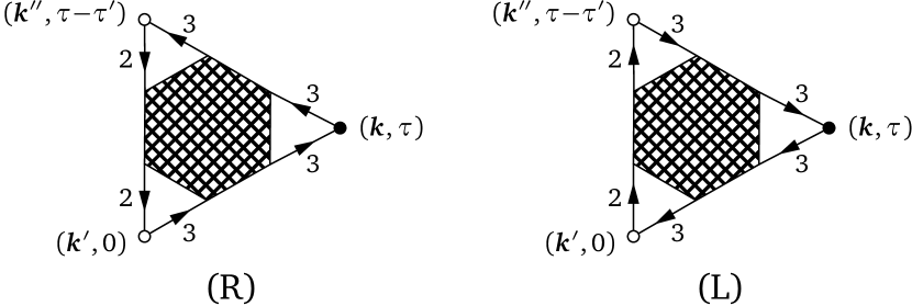
Figure 2: Diagrammatic representation of the double-imaginary time function (11). Diagrams (R) and (L) correspond to the first and second terms of Eq. (13), respectively, up to a minus sign (the correlation function equals minus the diagram, if standard diagrammatic rules are used). The two diagrams are identical, except for the direction of the arrows (R, right-handed, L, left-handed). The white dots denote the interaction of atoms with light, leading to transitions between internal states $|2\rangle$ and $|3\rangle$; the black dots denote the measured momentum distribution, and the hatched regions represent all interactions, including interactions with the state $|1\rangle$.

II.3 Leading contribution

We can distinguish two categories of diagrams, as illustrated in Fig. 3. The justification for separating the diagrams of type I from “vertex corrections” of type II stems from the fact that, in usual experimental conditions, the interactions in the final state are small compared with the other interactions. If the former are exactly zero ($V_{13}=V_{23}=V_{33}=0$), all vertex corrections of type II disappear. Then, the two diagrams of type I^′ (right- and left-handed) are the only nonvanishing terms, with the two propagators in state $3$ given by free propagators. Since diagram (I^′) can be derived from diagram (I) by taking the appropriate limit, we shall evaluate here diagram (I) and discuss the case of a noninteracting final state in the next section. Final-state effects are present in both type-I and type-II diagrams. We discuss final-state effects of type I in Secs. IV.1 and IV.2 and those of type II in Sec. IV.3.

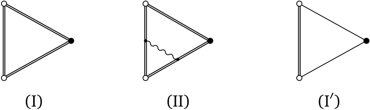
Figure 3: Leading term (I) and an example of vertex correction (II). In both cases, the two topologically inequivalent diagrams of kinds R and L must be considered. For a noninteracting final state, diagrams of type I^′ are the only nonvanishing contributions. Double lines denote the Green’s function, and single lines denote the noninteracting Green’s function in the final state.

The two diagrams of type I involve a single momentum, i.e., $\mathscr{C}_{n_{\bm{k}}\gamma_{\bm{k}^{\prime}}\gamma_{\bm{k}^{\prime\prime}}}^{\text{(I)}}(\tau,\tau^{\prime})\propto\delta_{\bm{k}\bm{k}^{\prime}}\delta_{\bm{k}\bm{k}^{\prime\prime}}$. They can be expressed in terms of the Green’s functions for each atomic state. We define the fermionic Green’s function as $\mathscr{G}_{\alpha}(\bm{k},\tau)=-\langle T_{\tau}c^{\phantom{\dagger}}_{\alpha\bm{k}}(\tau)c^{\dagger}_{\alpha\bm{k}}(0)\rangle_{H}$. In imaginary frequency, they are

$$\mathscr{G}_{1,2}(\bm{k},i\omega_{n}) =\frac{1}{i\omega_{n}-\xi_{\bm{k}}-\Sigma_{1,2}(\bm{k},i\omega_{n})}$$ (14)

$$\mathscr{G}_{3}(\bm{k},i\omega_{n}) =\frac{1}{i\omega_{n}-\xi_{\bm{k}}-h\nu_{0}-\Sigma_{3}(\bm{k},i\omega_{n})},$$ (15)

where $i\omega_{n}=(2n+1)\pi k_{\text{B}}T$, $\xi_{\bm{k}}=\varepsilon_{\bm{k}}-\mu$, and $\Sigma_{\alpha}(\bm{k},i\omega_{n})$ is the self-energy. Translating the two diagrams using the conventions of Fig. 2 gives

$$\mathscr{C}_{n_{\bm{k}}\gamma_{\bm{k}}\gamma_{\bm{k}}}^{\text{(I)}}(\tau,\tau^{\prime})=\mathscr{G}_{2}(\bm{k},\tau^{\prime}-\tau)\mathscr{G}_{3}(\bm{k},\tau)\mathscr{G}_{3}(\bm{k},-\tau^{\prime})\\ +\mathscr{G}_{2}(\bm{k},\tau-\tau^{\prime})\mathscr{G}_{3}(\bm{k},\tau^{\prime})\mathscr{G}_{3}(\bm{k},-\tau).$$ (16)

The minus sign associated with the fermion loop is canceled because the correlation function equals minus the diagram. We perform the Fourier transform in Eq. (12) using the spectral representation of the Green’s function,

$$\mathscr{G}_{\alpha}(\bm{k},\tau)=\int_{-\infty}^{\infty}d\varepsilon\,A_{\alpha}(\bm{k},\varepsilon)\frac{1}{\beta}\sum_{i\omega_{n}}\frac{e^{-i\omega_{n}\tau}}{i\omega_{n}-\varepsilon},$$ (17)

where $A_{\alpha}(\bm{k},\varepsilon)=-\text{Im}\,\mathscr{G}_{\alpha}(\bm{k},i\omega_{n}\to\varepsilon+i0^{+})/\pi$ is the single-particle spectral function. This leads to

$$\mathscr{C}_{n_{\bm{k}}\gamma_{\bm{k}}\gamma_{\bm{k}}}^{\text{(I)}}(i\Omega_{n},i\Omega_{n}^{\prime})=\int_{-\infty}^{\infty}d\varepsilon d\varepsilon^{\prime}d\varepsilon^{\prime\prime}\\ \times A_{2}(\bm{k},\varepsilon)\,A_{3}(\bm{k},\varepsilon^{\prime})\,A_{3}(\bm{k},\varepsilon^{\prime\prime})\\ \times\frac{1}{\beta}\sum_{i\omega_{n}}\frac{1}{i\omega_{n}-\varepsilon}\left[\frac{1}{i\omega_{n}+i\Omega_{n}-\varepsilon^{\prime}}\frac{1}{i\omega_{n}-i\Omega_{n}^{\prime}-\varepsilon^{\prime\prime}}\right.\\ \left.+\frac{1}{i\omega_{n}-i\Omega_{n}-\varepsilon^{\prime}}\frac{1}{i\omega_{n}+i\Omega_{n}^{\prime}-\varepsilon^{\prime\prime}}\right].$$ (18)

The frequency sums are evaluated in the usual manner Mahan (2000) and yield terms proportional to either $f(\varepsilon)$, $f(\varepsilon^{\prime})$, or $f(\varepsilon^{\prime\prime})$. For weak interactions in the final state, $A_{3}(\bm{k},\varepsilon)$ peaks near $\varepsilon=\xi_{\bm{k}}+h\nu_{0}$. The terms proportional to $f(\varepsilon^{\prime})$, and $f(\varepsilon^{\prime\prime})$ are therefore small at low temperature, like the zeroth-order term (6). We denote $\mathscr{C}_{n_{\bm{k}}\gamma_{\bm{k}}\gamma_{\bm{k}}}^{\text{(Ia)}}$ the contribution of the dominant terms proportional to $f(\varepsilon)$ and $\mathscr{C}_{n_{\bm{k}}\gamma_{\bm{k}}\gamma_{\bm{k}}}^{\text{(Ib)}}$ the contribution of the other terms. We have

$$\mathscr{C}_{n_{\bm{k}}\gamma_{\bm{k}}\gamma_{\bm{k}}}^{\text{(Ia)}}(i\Omega_{n},i\Omega_{n}^{\prime})=\int_{-\infty}^{\infty}d\varepsilon d\varepsilon^{\prime}d\varepsilon^{\prime\prime}\\ \times A_{2}(\bm{k},\varepsilon)\,A_{3}(\bm{k},\varepsilon^{\prime})\,A_{3}(\bm{k},\varepsilon^{\prime\prime})\\ \times f(\varepsilon)\left[\frac{1}{i\Omega_{n}+\varepsilon-\varepsilon^{\prime}}\frac{-1}{i\Omega_{n}^{\prime}-\varepsilon+\varepsilon^{\prime\prime}}\right.\\ \left.+\frac{-1}{i\Omega_{n}-\varepsilon+\varepsilon^{\prime}}\frac{1}{i\Omega_{n}^{\prime}+\varepsilon-\varepsilon^{\prime\prime}}\right].$$ (19)

Making the analytic continuation as in Eq. (10), and inserting in Eq. (9), we obtain the leading contribution to the momentum distribution:

$$\langle n_{\bm{k}}(t)\rangle^{\text{(Ia)}}=\int_{-\infty}^{\infty}d\varepsilon\,A_{2}(\bm{k},\varepsilon)\,f(\varepsilon)\\ \times\scalebox{1.0}[1.3]{\Big{|}}\int_{-\infty}^{\infty}\!\!d\varepsilon^{\prime}\,A_{3}(\bm{k},\varepsilon^{\prime})\mathscr{F}_{t}(\varepsilon-\varepsilon^{\prime})\scalebox{1.0}[1.3]{\Big{|}}^{2}.$$ (20)

The dimensionless function $\mathscr{F}$ accounts for the broadening effect due to the rf pulse:

$$\mathscr{F}_{t}(\varepsilon)=\int_{-\infty}^{\infty}\frac{d\omega}{2\pi}\frac{e^{-i\omega t}\mathscr{E}(\omega)}{\hbar\omega-\varepsilon+i0^{+}}=\frac{-i}{\hbar}\int_{-\infty}^{t}dt^{\prime}\,e^{i\frac{\varepsilon}{\hbar}(t^{\prime}-t)}\mathscr{E}(t^{\prime}).$$ (21)

The main goal of rf spectroscopy is to determine the spectral function $A_{2}(\bm{k},\varepsilon)$. For weak interactions, this function is peaked near $\varepsilon=\varepsilon_{\bm{k}}-\mu=\xi_{\bm{k}}$. On the other hand, since the dispersions in the initial and final states are the same and only $\bm{q}=0$ transitions are possible, one expects to observe, by varying the frequency $\nu$ of the rf radiation, a signal peaking close to the frequency $\nu_{0}$ of the noninteracting transition. In order to make this more apparent, we introduce the detuning $\tilde{\nu}=\nu_{0}-\nu$, we change variables in Eq. (20), and rewrite it in the form

$$\langle n_{\bm{k}}(t)\rangle^{\text{(Ia)}}=\int_{-\infty}^{\infty}d\varepsilon\,\mathscr{R}_{\bm{k}}^{\text{(Ia)}}(\varepsilon)\,A_{2}(\bm{k},\xi_{\bm{k}}+h\tilde{\nu}-\varepsilon)\\ \times f(\xi_{\bm{k}}+h\tilde{\nu}-\varepsilon).$$ (22a)

This shows that the measured momentum distribution is the convolution of the occupied part of the spectral function with a dimensionless resolution function $$\mathscr{R}_{\bm{k}}^{\text{(Ia)}} \delta(\varepsilon) \nu=\nu_{0}$$. Under ideal conditions, the resolution function is proportional to , and the momentum distribution peaks near , as expected. The expression of the resolution function resulting from Eq. (20) is

$$\mathscr{R}_{\bm{k}}^{\text{(Ia)}}(\varepsilon)=\scalebox{1.0}[1.3]{\Big{|}}\int_{-\infty}^{\infty}d\varepsilon^{\prime}\,A_{3}(\bm{k},\varepsilon^{\prime})\mathscr{F}_{t}(\varepsilon+\varepsilon^{\prime}-\xi_{\bm{k}}-h\tilde{\nu})\scalebox{1.0}[1.3]{\Big{|}}^{2}.$$ (22b)

It takes into account the renormalization of the final state by interactions, as well as the broadening due to the time envelope of the rf pulse. For a noninteracting final state with a spectral function $A_{3}(\bm{k},\varepsilon)=\delta(\varepsilon-\xi_{\bm{k}}-h\nu_{0})$, the resolution function simplifies to

$$\mathscr{R}^{\text{(I${}^{\prime}$)}}(\varepsilon)=\frac{1}{\hbar^{2}}\scalebox{1.0}[1.3]{\Big{|}}\int_{-\infty}^{t}dt^{\prime}\,e^{i(\varepsilon+h\nu)t^{\prime}/\hbar}\mathscr{E}(t^{\prime})\scalebox{1.0}[1.3]{\Big{|}}^{2}.$$ (23)

Equations (22) are one central result of this work. We use them to study the interplay of Hartree shifts and inhomogeneity in two-dimensional ⁴⁰K (Sec. III.2) and three-dimensional ⁶Li (Sec. III.3) and to study the effect of a finite lifetime in the final state (Sec. IV.1).

The terms resulting from the frequency sum in Eq. (18), which have not been retained in Eq. (19), are

$$\mathscr{C}_{n_{\bm{k}}\gamma_{\bm{k}}\gamma_{\bm{k}}}^{\text{(Ib)}}(i\Omega_{n},i\Omega_{n}^{\prime})=\int_{-\infty}^{\infty}d\varepsilon d\varepsilon^{\prime}d\varepsilon^{\prime\prime}\\ \times A_{2}(\bm{k},\varepsilon)A_{3}(\bm{k},\varepsilon^{\prime})A_{3}(\bm{k},\varepsilon^{\prime\prime})\\ f(\varepsilon^{\prime})\left[\left(\frac{1}{i\Omega_{n}+\varepsilon-\varepsilon^{\prime}}+\frac{1}{i\Omega_{n}^{\prime}+\varepsilon-\varepsilon^{\prime}}\right)\frac{1}{i\Omega_{n}+i\Omega_{n}^{\prime}-\varepsilon^{\prime}+\varepsilon^{\prime\prime}}\right.\\ \left.+\left(\frac{1}{i\Omega_{n}-\varepsilon+\varepsilon^{\prime}}+\frac{1}{i\Omega_{n}^{\prime}-\varepsilon+\varepsilon^{\prime}}\right)\frac{1}{i\Omega_{n}+i\Omega_{n}^{\prime}+\varepsilon^{\prime}-\varepsilon^{\prime\prime}}\right].$$ (24)

We have rearranged the terms by exchanging $\varepsilon^{\prime}$ and $\varepsilon^{\prime\prime}$ in half of them. We proceed as above, and introduce again a resolution function:

$$\langle n_{\bm{k}}(t)\rangle^{\text{(Ib)}}=-f(\xi_{\bm{k}}+h\nu_{0})\int_{-\infty}^{\infty}d\varepsilon\,\mathscr{R}_{\bm{k}}^{\text{(Ib)}}(\varepsilon)\\ \times A_{2}(\bm{k},\xi_{\bm{k}}+h\tilde{\nu}-\varepsilon).$$ (25a)

We have pulled out a minus sign, because this term is negative: It corresponds to a reduction of the thermal population in the final state as given by Eq. (6), induced by transitions to the initial state. These terms describe an inverse rf spectroscopy analogous to the inverse photoemission in condensed-matter systems. In the usual experimental practice, they do not contribute because the atom cloud is prepared in a slightly out-of-equilibrium state, where level $$|3\rangle$$ is empty. The resolution function in Eq. (25) is

$$\mathscr{R}_{\bm{k}}^{\text{(Ib)}}(\varepsilon)=\frac{2}{\hbar^{2}}\int_{-\infty}^{\infty}d\varepsilon^{\prime}d\varepsilon^{\prime\prime}\frac{f(\xi_{\bm{k}}+h\tilde{\nu}-\varepsilon^{\prime})}{f(\xi_{\bm{k}}+h\nu_{0})}\\ \times A_{3}(\bm{k},\xi_{\bm{k}}+h\tilde{\nu}-\varepsilon^{\prime})\,A_{3}(\bm{k},\xi_{\bm{k}}+h\tilde{\nu}-\varepsilon^{\prime\prime})\\ \times\text{Re}\,\int_{-\infty}^{t}\!\!dt^{\prime}\,e^{i\frac{\varepsilon-\varepsilon^{\prime\prime}}{\hbar}(t-t^{\prime})}\mathscr{E}(t^{\prime})\int_{-\infty}^{t^{\prime}}\!\!dt^{\prime\prime}\,e^{-i\frac{\varepsilon-\varepsilon^{\prime}}{\hbar}(t-t^{\prime\prime})}\mathscr{E}(t^{\prime\prime}).$$ (25b)

For a noninteracting final state, $\varepsilon^{\prime}$ and $\varepsilon^{\prime\prime}$ are both equal to $-h\nu$. The upper limit of the $t^{\prime\prime}$ integral can be extended from $t^{\prime}$ to $t$, correcting with a factor $1/2$. This shows that Eq. (25b) reduces to Eq. (23) and that the two resolution functions are equal for a noninteracting final state. We finally note that, if $t=+\infty$—i.e., if the measurement of the momentum distribution is performed after the extinction of the rf pulse—the resolution functions are simply given by

$$\mathscr{R}^{\text{(I${}^{\prime}$)}}(\varepsilon)=\frac{1}{\hbar^{2}}\left|\mathscr{E}(\varepsilon/\hbar+2\pi\nu)\right|^{2},$$ (26)

with $\mathscr{E}(\omega)$ the Fourier transform of $\mathscr{E}(t)$.

III Noninteracting final state

In this section, we neglect the interaction between the final state $|3\rangle$ and states $|1\rangle$ and $|2\rangle$ ($V_{13}=V_{23}=V_{31}=V_{32}=0$). We furthermore restrict to a short-range interaction such that $V_{\alpha\alpha}=0$. The atoms are free fermions in the final state, and the nonzero matrix elements are $V_{12}=V_{21}$, describing the short-range interaction between the states $|1\rangle$ and $|2\rangle$. In this limit, diagram (I^′) in Fig. 3 gives the whole second-order response, and the momentum distribution is the sum of Eqs. (7), (22), and (25). Because the spectral function in the final state is a $\delta$ function, both resolution functions are given by Eq. (23). In the context of electron photoemission, an analogous model known as the “sudden approximation” assumes a free-electron final state. In contrast to rf spectroscopy for cold atoms, however, this remains an approximation even in the ideal situation of a truly noninteracting final state, because other effects (in particular the surface) are usually neglected as well.

We consider a monochromatic radiation of frequency $\nu$ with a slowly varying envelope, such that the coupling in Eq. (3) is $\mathscr{E}(t)=\bar{\mathscr{E}}(t)\cos(2\pi\nu t).$ Assuming that the momentum distribution is measured after the end of the pulse, and that the duration of the pulse is much longer than $1/\nu$, the resolution function is $\mathscr{R}^{\text{(I${}^{\prime}$)}}(\varepsilon)=|\bar{\mathscr{E}}(\varepsilon/\hbar)|^{2}/(4\hbar^{2})$ with $\bar{\mathscr{E}}(\omega)$ the Fourier transform of $\bar{\mathscr{E}}(t)$. For a square pulse of intensity $\mathscr{E}_{0}$ and duration $\Delta\nu^{-1}$ in the limit $\nu\gg\Delta\nu$, the resolution function is

$$\mathscr{R}^{\text{(I${}^{\prime}$)}}(\varepsilon)=\left(\frac{\pi\mathscr{E}_{0}}{h\Delta\nu}\right)^{2}\left[\frac{\sin(\pi x)}{\pi x}\right]^{2},\quad x=\frac{\varepsilon}{h\Delta\nu}.$$ (27)

For a Gaussian pulse of the same intensity at the maximum and a full width at half maximum $\Delta\nu^{-1}$ we have

$$\mathscr{R}^{\text{(I${}^{\prime}$)}}(\varepsilon)=\left(\frac{\pi\mathscr{E}_{0}}{h\Delta\nu}\right)^{2}\frac{\pi}{4\ln 2}\exp\left[-\frac{(\pi x)^{2}}{\ln 4}\right].$$ (28)

The two functions are compared in Fig. 4. The validity of any approach based on equilibrium response is limited to a regime where the fraction of atoms transferred to the final state is small, or equivalently, the time $t$ of the measurement is short compared with $2h/\mathscr{E}_{0}$, which is the period of Rabi oscillations between the states $|2\rangle$ and $|3\rangle$. Since, on the other hand, $t\gtrsim\Delta\nu^{-1}$, this regime corresponds to $\mathscr{E}_{0}/(2h\Delta\nu)\ll 1$. Our formalism is therefore valid as long as the amplitude of the resolution function is much smaller than unity.

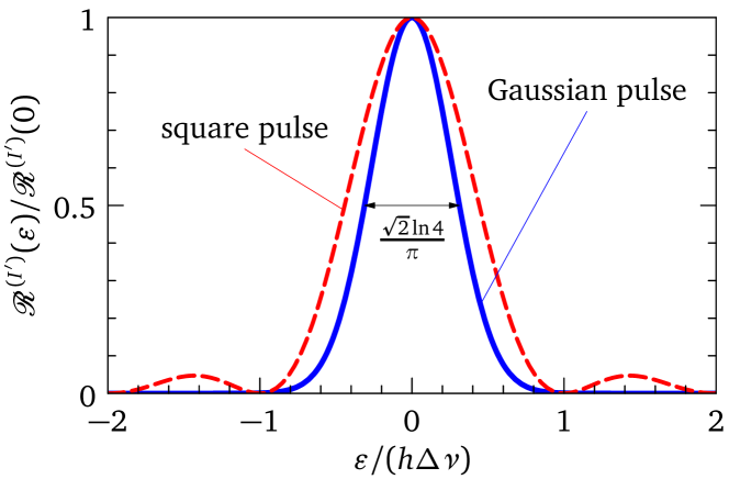
Figure 4: (Color online) Resolution function for a rf pulse with a square (dashed line) and Gaussian (solid line) envelope in the case of a noninteracting final state. The width of the envelope in the time domain is fixed by $\Delta\nu^{-1}$ in both cases (full width at half maximum in the Gaussian case). The curves are normalized to the peak maximum for easier comparison.

III.1 Free and nearly free fermions in a harmonic trap

If all interactions are turned off, the spectral function is $A_{2}(\bm{k},\varepsilon)=\delta(\varepsilon-\xi_{\bm{k}})$. For a homogeneous fermion gas, the momentum distribution is therefore simply

$$\langle n_{\bm{k}}\rangle=\mathscr{R}^{\text{(I${}^{\prime}$)}}(h\tilde{\nu})f(\xi_{\bm{k}})\\ +[1-\mathscr{R}^{\text{(I${}^{\prime}$)}}(h\tilde{\nu})]f(\xi_{\bm{k}}+h\nu_{0}).$$ (29)

The first term corresponds to the atoms excited from the initial state, while the second term corresponds to the equilibrium thermal population of the final state, reduced by the transitions to the initial state. From here on, we assume that $h\nu_{0}$ is large enough for the second term in Eq. (29) to be negligible. Equation (29) indicates that one can, in principle, determine the frequency $\nu_{0}$ of the noninteracting transition, the resolution $\Delta\nu$, and the temperature $T$ by measuring the momentum distribution with all interactions suppressed: the energy-distribution curve (EDC) is just the resolution function, while the momentum-distribution curve (MDC) is controlled by the Fermi function. Experiments with homogeneous Fermi gases have not been conducted yet (for bosons, see Ref. Gaunt et al., 2013). In this section, we study within LDA the modifications of Eq. (29) due to the nonhomogeneous distribution of atoms trapped in a harmonic potential, in two and three dimensions. The resulting equations provide a way of determining the total number of atoms, in addition to $\nu_{0}$, $\Delta\nu$, and $T$, by fitting experimental EDCs and MDCs.

Consider a harmonic trap described by the potential $V(r)=(1/2)m\omega_{r}^{2}r^{2}$. In dimension $d$, the number of atoms in state $|1\rangle$ is related to the chemical potential by

$$N_{1}=\int d^{d}r\int\frac{d^{d}k}{(2\pi)^{d}}\frac{1}{e^{\beta(\varepsilon_{\bm{k}}-\mu+\frac{1}{2}m\omega_{r}^{2}r^{2})}+1}.$$ (30)

For free particles with a dispersion $\varepsilon_{\bm{k}}=\hbar^{2}k^{2}/(2m)$, the evaluation of the integrals gives

$$N_{1}=-\left(\frac{k_{\text{B}}T}{\hbar\omega_{r}}\right)^{d}\text{Li}_{d}\left(-e^{\frac{\mu}{k_{\text{B}}T}}\right),$$ (31)

where $\text{Li}_{2}$ and $\text{Li}_{3}$ are the di- and trilogarithm, respectively. Note that, unlike Eq. (31) suggests, $\mu$ does depend on the particle mass $m$, because $\omega_{r}=(\kappa/m)^{1/2}$, where $\kappa$ is the strength of the harmonic potential. To estimate the trap-averaged momentum distribution, we replace $f(\xi_{\bm{k}})$ in Eq. (29) with $f\big{(}\varepsilon_{\bm{k}}-\mu+V(r)\big{)}$, and we perform a spatial integration. The result is

$$\langle n_{\bm{k}}\rangle_{\text{LDA}}=-\left(\frac{2\pi k_{\text{B}}T}{m\omega_{r}^{2}}\right)^{\frac{d}{2}}\text{Li}_{\frac{d}{2}}\left(-e^{\frac{\mu-\varepsilon_{\bm{k}}}{k_{\text{B}}T}}\right)\mathscr{R}^{\text{(I${}^{\prime}$)}}(h\tilde{\nu}).$$ (32)

Note that $\langle n_{\bm{k}}\rangle_{\text{LDA}}$ is extensive and has the units of a normalization volume. Equation (32) shows that for free particles in the LDA, the EDCs are not affected by the inhomogeneities, because the latter do not change the energy of the $|2\rangle\to|3\rangle$ transition. The measured EDC line shape depends neither on the details of the density distribution in the trap nor on the momentum, but is entirely determined by the properties of the rf pulse.

A qualitative understanding of the effects of interactions on the EDC and MDC curves may be gained by considering nearly free fermions. The simplest model is that of free fermions with an effective mass $m^{*}$. With the caveat that such a model can only be envisioned as a low-energy idealization, this effective mass can be simulated by assuming for the bare fermions a self-energy,

$$\Sigma_{\bm{k}}=\frac{\hbar^{2}k^{2}}{2}\left(\frac{1}{m^{*}}-\frac{1}{m}\right),$$ (33)

such that $\varepsilon_{\bm{k}}+\Sigma_{\bm{k}}=\hbar^{2}k^{2}/(2m^{*})\equiv E_{\bm{k}}$, and the spectral function of the initial state is $A_{2}(\bm{k},\varepsilon)=\delta(\varepsilon-\xi_{\bm{k}}-\Sigma_{\bm{k}})$. Neglecting the population of the final state, the corresponding momentum distribution for a homogeneous gas is

$$\langle n_{\bm{k}}\rangle=\mathscr{R}^{\text{(I${}^{\prime}$)}}(h\tilde{\nu}-\Sigma_{\bm{k}})f(E_{\bm{k}}-\mu).$$ (34)

The maximum of the EDC is at $h(\nu_{0}-\nu)=\Sigma_{\bm{k}}$, and tracks the difference in the dispersions of the initial and final states. The dispersion of the EDC maximum is given by $E_{\text{max}}(k)=(\hbar^{2}k^{2}/2)(1/m^{*}-1/m)$. This means that, for $m^{*}>m$, the peak moves towards lower values of the detuning $\nu_{0}-\nu$ with increasing momentum $k$.

Like for free fermions, the inhomogeneities due to trapping do not affect the EDC line shape for nearly free fermions, because the self-energy (33) does not depend on the local atom density. In such a gas, a plot of the quadratic EDC peak dispersion as a function of $k$ gives the effective mass. The MDC profile also reflects the effective mass. Equation (31) gets corrected by a factor $(m^{*}/m)^{d/2}$ because $\omega_{r}$ is defined in terms of the bare mass; in Eq. (32), the changes $\varepsilon_{\bm{k}}\to E_{\bm{k}}$ and $h\tilde{\nu}\to h\tilde{\nu}-\Sigma_{\bm{k}}$ must be made in order to describe harmonically trapped nearly free fermions.

III.2 EDC dispersion due to inhomogeneity and Hartree shifts

For free and nearly free fermions, the EDC line shape is not modified by the inhomogeneity, and the dispersion of the EDC peak tracks the intrinsic quasiparticle dispersion. However, if the self-energy depends on density, these convenient properties are lost. In order to illustrate this in the simplest model, we consider the case of fermions subject to a short-range interaction, which is treated to lowest order, by keeping only the Hartree term. The momentum- and energy-independent Hartree self-energy in state $|2\rangle$ is given by

$$\Sigma_{2}=(g/N_{0})n_{1},$$ (35)

with $n_{1}$ the density of atoms in state $|1\rangle$. The state $|1\rangle$ experiences a similar shift $\Sigma_{1}=(g/N_{0})n_{2}$. The dimensionless coupling $g$ is positive (negative) for repulsive (attractive) interaction, and $N_{0}$ is the Fermi-level DOS, given by $mk_{\text{F}}/(2\pi^{2}\hbar^{2})$ and $m/(2\pi\hbar^{2})$ in three and two dimensions, respectively. The coupling $g$ is related to the scattering length via $g/N_{0}=4\pi\hbar^{2}a_{\text{3D}}/m$ and $g=-1/\ln(k_{\text{F}}a_{\text{2D}})$ in 3D and 2D, respectively. Equation (35) means that the energy of the transition is reduced (increased) with respect to the noninteracting value $h\nu_{0}$ for a repulsive (attractive) interaction. In a harmonic trap, the modification varies from the center to the periphery, and this contributes to a broadening and a momentum dependence of the EDC, resulting in a dispersion of the EDC peak, as we shall see. This dispersion may by qualified “spurious”, because it is observed in a system where the transition does not actually disperse with momentum.

With the Hartree term (35), the spectral function is $A_{2}(\bm{k},\varepsilon)=\delta(\varepsilon-\xi_{\bm{k}}-\Sigma_{2})$. For a homogeneous gas of density $n_{1}$, the chemical potential is set by the self-consistency condition

$$n_{1}=\int\frac{d^{d}k}{(2\pi)^{d}}\int_{-\infty}^{\infty}d\varepsilon\,A_{1}(\bm{k},\varepsilon)f(\varepsilon)\\ =-\left(\frac{mk_{\text{B}}T}{2\pi\hbar^{2}}\right)^{\frac{d}{2}}\text{Li}_{\frac{d}{2}}\left(-e^{\frac{\mu-(g/N_{0})n_{2}}{k_{\text{B}}T}}\right),$$ (36)

and the momentum distribution (22) becomes

$$\langle n_{\bm{k}}\rangle=\mathscr{R}^{\text{(I${}^{\prime}$)}}(h\tilde{\nu}-\Sigma_{2})f(\xi_{\bm{k}}+\Sigma_{2}).$$ (37)

In a harmonic trap, the local self-consistency condition reads

$$n_{1}(\bm{r})=-\left(\frac{mk_{\text{B}}T}{2\pi\hbar^{2}}\right)^{\frac{d}{2}}\text{Li}_{\frac{d}{2}}\left(-e^{\frac{\mu-\frac{1}{2}m\omega_{r}^{2}r^{2}-(g/N_{0})n_{2}(\bm{r})}{k_{\text{B}}T}}\right),$$ (38)

where $\mu$ is fixed by the condition $N_{1}=\int d^{d}r\,n_{1}(\bm{r})$. The explicit expression for the momentum distribution in the harmonic trap is therefore

$$\langle n_{\bm{k}}\rangle_{\text{LDA}}=\int d^{d}r\,\frac{\mathscr{R}^{\text{(I${}^{\prime}$)}}\big{(}h\tilde{\nu}-(g/N_{0})n_{1}(\bm{r})\big{)}}{\exp\left(\frac{\varepsilon_{\bm{k}}-\mu+\frac{1}{2}m\omega_{r}^{2}r^{2}+(g/N_{0})n_{1}(\bm{r})}{k_{\text{B}}T}\right)+1}.$$ (39)

Figure 5 shows the EDCs calculated using Eq. (39), in a two-dimensional gas of ⁴⁰K atoms with $n_{1}=n_{2}\equiv n$, and using parameters typical for the experiment of Ref. Fröhlich et al., 2012. The maximum of the EDC disperses towards lower (higher) values of $\nu_{0}-\nu$ for attractive (repulsive) interaction. The width of the EDC varies with momentum and is larger than the expected resolution, which is $\Delta\nu\sqrt{2}\ln 4/\pi=3.12$ kHz.

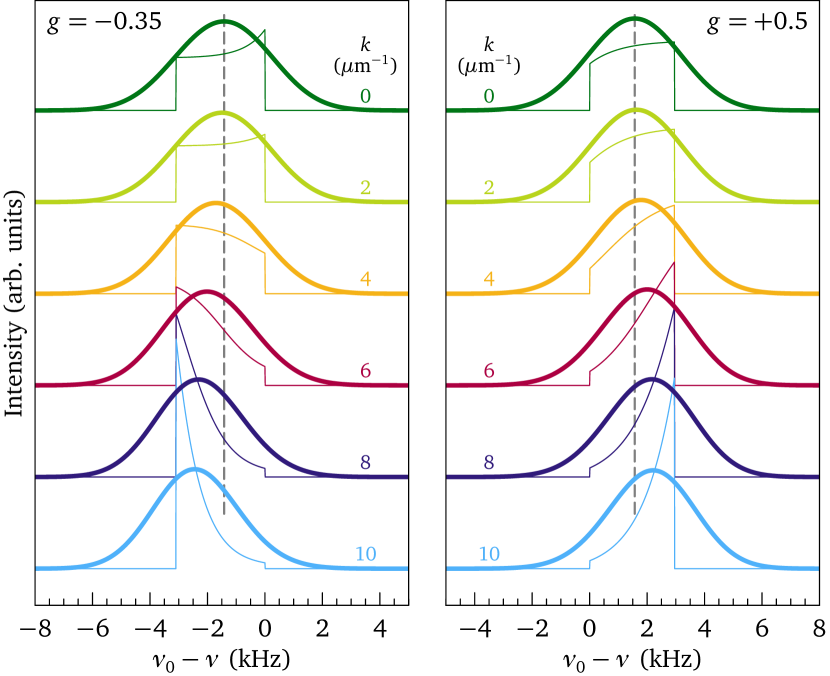
Figure 5: (Color online) Energy-distribution curves for harmonically trapped ⁴⁰K atoms in two dimensions: effect of the Hartree shift. The EDC (39) for a Gaussian pulse with $\Delta\nu=5$ kHz are normalized and shown at different momenta (thick lines), for attractive (left) and repulsive (right) interaction. The thin lines show the intrinsic EDC corresponding to each curve [$\Delta\nu=0$, Eq. (40)], divided by two for clarity. The other parameters are $\omega_{r}/2\pi=127$ Hz, $N_{1}=2000$, and $T=100$ nK.

The curves for attractive and repulsive interaction look similar in Fig. 5; however, the magnitudes of $g$ are different. In fact, there is a systematic asymmetry between positive and negative $g$, because an attractive interaction tends to gather atoms near the center of the trap, leading to a more inhomogeneous density [see Fig. 7(a)]. The width of the EDC reflects the distribution of densities in the trap. This distribution is defined as $D(\mathfrak{n})=\int d^{d}r\,\delta\big{(}\mathfrak{n}-n(\bm{r})\big{)}$, and takes nonzero values for densities $\mathfrak{n}$ between $0$ and $n(0)$. As shown in Appendix B, it is possible to rewrite the momentum distribution (39) as an integral over densities involving $D(\mathfrak{n})$ [Eq. (64)]. In dimension $d=2$, the distribution $D(\mathfrak{n})$ can be evaluated explicitly (see Appendix B). For an ideal resolution, the resulting momentum distribution is

$$\langle n_{\bm{k}}\rangle_{\text{LDA}}\propto\begin{cases}\displaystyle\frac{1+g+b\left(\frac{h\tilde{\nu}}{g}\right)}{1+e^{\beta\varepsilon_{k}}b\left(\frac{h\tilde{\nu}}{g}\right)}&0\leqslant\frac{h\tilde{\nu}}{g}\leqslant\frac{n(0)}{N_{0}}\vspace{2mm}\\ 0&\text{otherwise,}\end{cases}$$ (40)

with $b(\varepsilon)=(e^{\beta\varepsilon}-1)^{-1}$. This is shown as the thin lines in Fig. 5 and corresponds to the $\Delta\nu\to 0$ limit of Eq. (39). The peculiar line shape (40), which depends on both the density distribution $D(\mathfrak{n})$ and the Fermi occupation factors, could be revealed experimentally by a moderate improvement of the resolution. Figure 6 shows the evolution of a typical line shape, as the full width at half maximum of the Gaussian rf pulse is increased from 0.2 to 1.0 ms.

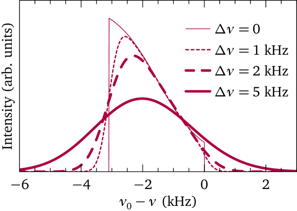
Figure 6: (Color online) Convergence of the measured EDC towards the intrinsic EDC (thin line) with improving the resolution by increasing the duration $\Delta\nu^{-1}$ of the Gaussian pulse. The EDCs are shown for $g=-0.35$ and $k=6~{}\mu\text{m}^{-1}$, with the same parameters as in Fig. 5.

The dispersion of the EDC maximum with increasing momentum is plotted in Fig. 7(b) for various interaction strengths and temperatures. This “spurious” dispersion may be understood as follows. At each point in the trap, the minimum of the local energy band is the sum of the harmonic potential and the Hartree term. The $k=0$ states are occupied throughout the trap and give contributions to the EDC with a Hartree shift ranging between 0 at the periphery and $(g/N_{0})n(0)$ at the center. The EDC for $k=0$ extends therefore from $\tilde{\nu}=0$ to $\tilde{\nu}=(g/N_{0})n(0)/h$. As the momentum increases, the corresponding $k$ states in the low-density regions at the periphery are above the chemical potential, and their thermal population contributes less to the intrinsic EDC. The latter is depressed near $\tilde{\nu}=0$ and becomes asymmetric. Once filtered with the resolution function, the observed EDC disperses as seen in Fig. 5. We can be more quantitative in the limit $T\to 0$, where the intrinsic EDC (40) becomes a rectangular distribution, constant for $\varepsilon_{k}\leqslant h\tilde{\nu}/g\leqslant n(0)/N_{0}$, and zero otherwise. Convolved with the resolution function, this distribution gives a peak whose maximum disperses quadratically: $E_{\text{max}}(k)=(g/2)[\varepsilon_{k}+n(0)/N_{0}]$. This dispersion can be parametrized by a Hartree “effective mass” $m_{\text{H}}$ as $E_{\text{max}}(k)-E_{\text{max}}(0)=(\hbar^{2}k^{2}/2)\left(1/m_{\text{H}}-1/m\right)$. We then find $m_{\text{H}}/m=1/(1+g/2)$. This is compared in Fig. 7(c) with the mass calculated numerically for various temperatures. The density at the trap center can also be evaluated at $T=0$: $n(0)/N_{0}=\hbar\omega_{r}\sqrt{2N_{1}/(1+g)}$.Note (1) With this, we can calculate the full $T=0$ dispersion, which is shown as thin lines in Fig. 7(b).

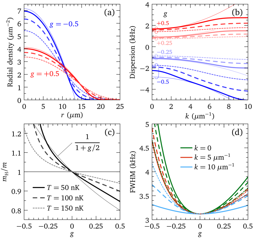
Figure 7: (Color online) (a) Radial density, (b) dispersion of the EDC maximum as a function of momentum, (c) Hartree “effective mass” as a function of $g$, and (d) width of the EDC. In all graphs, dotted lines correspond to $T=150$ nK, dashed lines to $T=100$ nK, thick solid lines to $T=50$ nK, and the thin solid lines give the analytical result for $T=0$ (see text). In (d), the width is shown as a function of $g$ for three momenta; the colors correspond to those used in Fig. 5. The model parameters are $\omega_{r}/2\pi=127$ Hz, $N_{1}=2000$, and $\Delta\nu=5$ kHz. The minimum at $g=0$ in (d) corresponds to the resolution of 3.12 kHz.

At finite $T$, the dispersion is not quadratic, except close to $k=0$, and for $g$ not too close to $-1$. As temperature increases, the particle cloud spreads more across the trap [see Fig. 7(a)], the density distribution $D(\mathfrak{n})$ sharpens, and the peak dispersion therefore gets weaker. The asymmetry between repulsive and attractive interaction is strongest at $T=0$ and is reduced as temperature increases. The finite-$T$ Hartree mass $m_{\text{H}}$, deduced from the curvature of the dispersion at $k=0$, is shown in Fig. 7(c). The relative mass is larger than unity for attractive interaction and smaller than unity for repulsive interaction. Its dependence on temperature is linear for $g>0$, but more complicated for $g<0$; in particular, nonlinearities in the temperature dependence get stronger as $g$ approaches $-1$, as can be seen in Figs. 7(b) and 7(c).

As seen in Fig. 5, the EDC not only disperses due to inhomogeneity, but also narrows with increasing momentum. At zero temperature, the width of the EDC has a complicated dependency on $\Delta\nu$, which approaches a linear function of $|g|$ as $\Delta\nu\to 0$, namely $|g/h(\varepsilon_{k}-n(0)/N_{0})|$. At finite temperature and finite resolution, however, the EDC width behaves more like $\sim g^{2}$, as shown in Fig. 7(d). At $k=0$, the width reflects the radial density distribution of Fig. 7(a): It is larger for attractive than for repulsive interaction of the same magnitudes and decreases with increasing temperature. The rounded behavior at $g=0$ transforms into a linear behavior $\sim|g|/\sqrt{1+g}$ as $\Delta\nu$ is reduced.Note (1) At large momenta, the width is controlled by the Fermi edge rather than by $D(\mathfrak{n})$: It is resolution-limited at low temperature and increases with increasing $T$.

The dispersion displayed in Figs. 5 and 7(b), as well as a width looking like $\sim g^{2}$ as seen in Fig. 7(d), could easily be mistaken as a signature of dynamical interactions, since this is the expected behavior in a homogeneous Fermi liquid. Even the narrowing of the EDC with increasing $k$ could evoke the sharpening of quasiparticles when approaching the Fermi momentum. One feature, however, among these inhomogeneity-driven effects is contrary to the expected signature of interactions: The sharpening of the $k=0$ EDC with increasing $T$, due to the flattening of the atom cloud in the trap, cannot be reconciled with the expected increase of the scattering rate with $T$ in an interacting system.

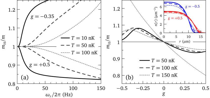
Figure 8: (Color online) (a) Evolution of the Hartree “effective mass” with $\omega_{r}$ for attractive (top curves) and repulsive (bottom curves) interaction and for three different temperatures. (b) Hartree “effective mass” as a function of $g$ for a $r^{4}$ trap and three temperatures. The thin solid line shows $1/(1+g/2)$ for easier comparison with Fig. 7(c). (Inset) Radial density for two values of $g$ and the same three temperatures.

An obvious way to reduce the spurious mass $m_{\text{H}}$ in experiments is to achieve a more homogeneous density. In three dimensions, this can be realized by means of a weaker confining harmonic potential. It does not work well in two dimensions, though, because the density distribution $D(\mathfrak{n})$ is flat at zero temperature: All densities between zero and the maximum density are equally represented, irrespective of the potential strength. This is illustrated by the fact that $m_{\text{H}}$ is given by $1/(1+g/2)$ at zero temperature, which does not depend on $\omega_{r}$. At finite $T$, $D(\mathfrak{n})$ does depend on $\mathfrak{n}$ (see Appendix B), and thus $m_{\text{H}}/m$ approaches unity as $\omega_{r}$ is reduced, as shown in Fig. 8(a). Alternatively, one may obtain a more homogeneous density by means of a quartic trapping potential. Figure 8(b) shows $m_{\text{H}}$ as a function of $g$ when the harmonic trap is replaced by a $r^{4}$ trap. The latter was defined such that the potential equals the harmonic potential with $\omega_{r}/2\pi=127$ Hz at a distance $r=10~{}\mu$m. The inset shows that the density profile is flatter than in Fig. 7(a), and as a result $m_{\text{H}}$ is significantly reduced as compared to Fig. 7(c). The spurious dispersion can also be reduced, and in some cases even suppressed, by taking advantage of interactions in the final state; this is discussed in Sec. IV.2.

III.3 Inhomogeneity and momentum-integrated rf intensity

In this paragraph we briefly discuss the effect of Hartree shifts and inhomogeneity on the momentum-integrated rf intensity. In the particular case of a Gaussian density profile, which is a good approximation for three-dimensional gases at not too low temperature, and a Gaussian rf pulse, the trap-averaged integrated intensity takes a universal form depending on a single parameter $\propto a_{\text{3D}}n(0)/(m\Delta\nu)$. We compare this form with the measurements of Ref. Gupta et al., 2003, where Hartree shifts in ⁶Li mixtures were studied by rf spectroscopy as a means to determine the scattering length.

The momentum integration of the rf intensity (39) yields

$$I_{\text{LDA}}=\int d^{d}r\,n_{2}(\bm{r})\,\mathscr{R}^{\text{(I${}^{\prime}$)}}\big{(}h\tilde{\nu}-(g/N_{0})n_{1}(\bm{r})\big{)}.$$ (41)

For a balanced gas with $n_{1}=n_{2}=n$, this becomes a one-dimensional integral involving the density distribution:

$$I_{\text{LDA}}=\int_{-\infty}^{\infty}d\mathfrak{n}\,D(\mathfrak{n})\,\mathfrak{n}\,\mathscr{R}^{\text{(I${}^{\prime}$)}}\big{(}h\tilde{\nu}-(g/N_{0})\mathfrak{n}\big{)}.$$ (42)

We are interested in comparing this expression with the data of Ref. Gupta et al., 2003, which were obtained at $T\sim 0.7T_{\text{F}}$. At such temperatures, the density profile given by Eq. (38) is very close to a Gaussian in three dimensions: $n(r)\approx n(0)\exp\big{\{}-\pi\left[n(0)/N_{1}\right]^{2/3}r^{2}\big{\}}$. For this Gaussian profile, the density distribution is

$$D(\mathfrak{n})=\begin{cases}\displaystyle\frac{2N_{1}\sqrt{\ln[n(0)/\mathfrak{n}]/\pi}}{n(0)\mathfrak{n}}&0\leqslant\mathfrak{n}\leqslant n(0)\vspace{2mm}\\ 0&\text{otherwise}.\end{cases}$$ (43)

If the rf pulse has a Gaussian envelope, Eq. (42) becomes

$$I_{\text{LDA}}\propto\mathscr{I}\left(\frac{gn(0)}{h\Delta\nu N_{0}},\frac{\tilde{\nu}}{\Delta\nu}\right)=\mathscr{I}\left(\frac{2\hbar a_{\text{3D}}n(0)}{m\Delta\nu},\frac{\tilde{\nu}}{\Delta\nu}\right),$$ (44)

where the function $\mathscr{I}$ is given by

$$\mathscr{I}(\alpha,x)=\int_{0}^{\infty}du\,\sqrt{u}\,e^{-u}\,\exp\left[-\frac{\pi^{2}}{\ln 4}(x-\alpha e^{-u})^{2}\right].$$ (45)

This function is displayed in Fig. 9(a). For $\alpha=0$, it is a Gaussian, and for $\alpha\neq 0$ it has an asymmetric shape with a cutoff at $x\approx\alpha$. Note that $\mathscr{I}(\alpha,x)=\mathscr{I}(-\alpha,-x)$, so that symmetric curves are expected for attractive and repulsive interactions corresponding to identical values of the product $|a_{\text{3D}}|n(0)$.

Equation (44) can be fit to the ⁶Li data as shown in Fig. 9(b). The function $\mathscr{I}$ captures remarkably well the peculiar asymmetry of the line shape in the presence of interactions (white dots), in contrast to the Gaussian used in Ref. Gupta et al., 2003, resulting in an excellent fit. We have set $\Delta\nu=7.1$ kHz, which corresponds to the Gaussian rf pulse of 140 $\mu$s used in this experiment. For the data without interaction (black dots), there is no further adjustable parameter, apart from the amplitude and a constant background. For the curve with interaction, the fit yields $\alpha=-7.15\pm 0.34$. Considering that the average density is $\bar{n}\sim 2.4\times 10^{13}$ cm^-3, and that $\bar{n}=n(0)/2^{3/2}$ for a Gaussian profile, this corresponds to a scattering length $a_{\text{3D}}=-35.4\pm 1.7$ nm. The analysis of Ref. Gupta et al., 2003 yields a value consistent within the error bars, $-31\pm 2.7$ nm, but we believe that Eq. (44) provides a more accurate way of measuring the scattering length.

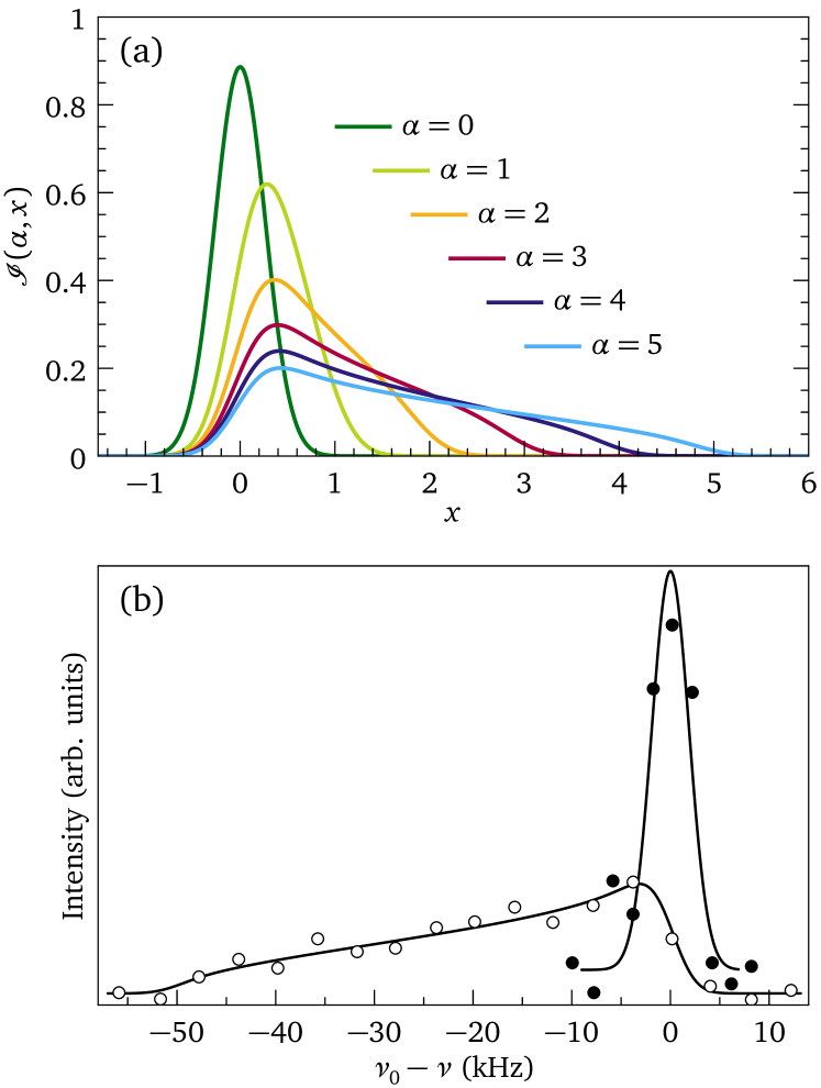
Figure 9: (Color online) (a) The function $\mathscr{I}(\alpha,x)$ defined in Eq. (45) for various values of $\alpha$. Note that the cutoff is at $x\approx\alpha$. (b) Data of Ref. Gupta et al., 2003 (dots) and fits to Eq. (44) with $\Delta\nu$ fixed to 7.1 kHz (lines). A constant background was added to Eq. (44) for fitting.

IV Discussion of final-state effects

IV.1 Resolution function for a Lorentzian final state

We start this section by deriving the modifications due to the resolution functions (23) and (28), in the situation where interactions lead to a shift and a lifetime for the final state of the rf transition. We introduce these effects by means of a phenomenological self-energy $\Sigma_{3}-i\Gamma_{3}$ in the final state, where $\Sigma_{3}$ is the energy shift and $\Gamma_{3}$ is the scattering rate. These two quantities are, in principle, related by causality and should be of the same order of magnitude for weak interactions. The corresponding lifetime of the final state is $\tau_{3}=\hbar/(2\Gamma_{3})$, and the spectral function reads

$$A_{3}(\bm{k},\varepsilon)=\frac{\Gamma_{3}/\pi}{(\varepsilon-\xi_{\bm{k}}-h\nu_{0}-\Sigma_{3})^{2}+\Gamma_{3}^{2}}.$$ (46)

The noninteracting result (23) gets modified like this:

$$\mathscr{R}^{\text{(Ia)}}(\varepsilon)=\frac{e^{-2\Gamma_{3}t/\hbar}}{\hbar^{2}}\scalebox{1.0}[1.3]{\Big{|}}\int_{-\infty}^{t}dt^{\prime}\,e^{i(\varepsilon+h\nu+\Sigma_{3}-i\Gamma_{3})t^{\prime}/\hbar}\mathscr{E}(t^{\prime})\scalebox{1.0}[1.3]{\Big{|}}^{2}.$$ (47)

The overall magnitude of the resolution function vanishes on time scales larger than $\tau_{3}$, because atoms in the final state decay. Besides, the energy dependence of the resolution function is also affected. In order to find out how, we perform the time integration explicitly for the case of a Gaussian pulse of full width at half maximum $\Delta\nu^{-1}$. In the relevant limit $\Delta\nu\ll\nu$, the formula replacing Eq. (28) is

$$\mathscr{R}^{(\text{Ia})}(\varepsilon)=\left(\frac{\pi\mathscr{E}_{0}}{h\Delta\nu}\right)^{2}\frac{\pi}{16\ln 2}\exp\left[\frac{\pi^{2}}{\ln 4}\left(\frac{\Gamma_{3}}{h\Delta\nu}\right)^{2}-\frac{2\Gamma_{3}t}{\hbar}\right]\\ \times\exp\left[-\frac{\pi^{2}}{\ln 4}\left(\frac{\varepsilon+\Sigma_{3}}{h\Delta\nu}\right)^{2}\right]\\ \times\left|1+\text{erf}\left(2\sqrt{\ln 2}\Delta\nu t-\frac{i\pi}{2\sqrt{\ln 2}}\frac{\varepsilon+\Sigma_{3}-i\Gamma_{3}}{h\Delta\nu}\right)\right|^{2}.$$ (48)

This complicated expression has an interesting time dependence (Fig. 10). The resolution function is even and centered at the energy $\varepsilon=-\Sigma_{3}$, and it is significantly non-Gaussian when the time delay $t$ of the measurement—counted in Eq. (48) from the maximum of the pulse envelope—is comparable to the width of the pulse. For large times $t\gg\Delta\nu^{-1}$, the erf function approaches one, and the energy dependence of Eq. (48) measured from $\varepsilon=-\Sigma_{3}$ is identical to the noninteracting result (28), shown in Fig. 10(a) as “Fourier limited”. The width of the resolution function takes off for measurement times of the order of $\Delta\nu^{-1}$ and increases roughly linearly with decreasing $t$ [Fig. 10(b)]. The peak intensity of $\mathscr{R}^{(\text{Ia})}(\varepsilon)$ is largest shortly after the pulse maximum and decreases for longer times [Fig. 10(c)].

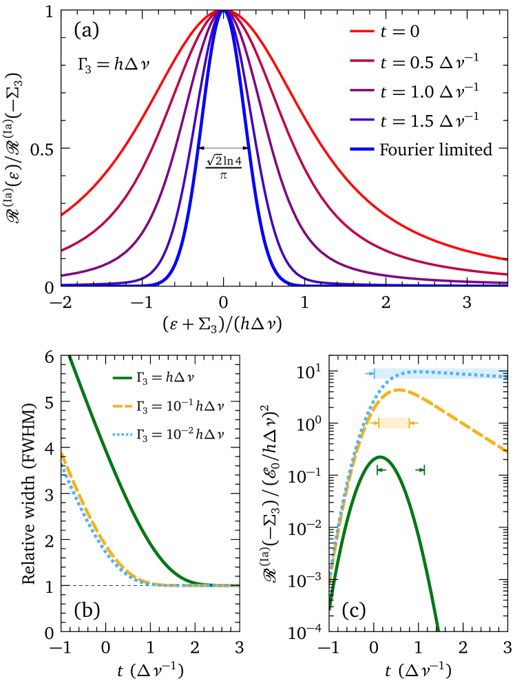
Figure 10: (Color online) (a) Energy dependence of the resolution function (48) for a final-state scattering rate $\Gamma_{3}=h\Delta\nu$, corresponding to a lifetime $\tau_{3}=\Delta\nu^{-1}/(4\pi)$, and for increasing measurement times (broader to narrower). The time $t$ is measured from the maximum of the Gaussian pulse envelope, such that $t=\Delta\nu^{-1}$ corresponds to a measurement time one full width after the pulse maximum. (b) Full width at half maximum of the resolution function relative to the Fourier limited value and (c) maximum intensity as a function of the measurement time and scattering rate. The arrows pointing to the left in (c) indicate the time $\tau_{3}$, and those pointing to the right the time $\frac{1}{16\ln 2\,\tau_{3}\Delta\nu}\Delta\nu^{-1}$.

Measurements can be done in the regime where the resolution function is Fourier limited, provided that the time $t$ is smaller than the lifetime $\tau_{3}$, but sufficiently large, that the real part of the argument in the erf function is large and positive. These requirements read

$$\frac{1}{16\ln 2\,\tau_{3}\Delta\nu}\Delta\nu^{-1}<t<\tau_{3}.$$ (49)

Clearly, such a regime does not exist unless $\tau_{3}\gg\Delta\nu^{-1}/(4\sqrt{\ln 2})$ or $\Gamma_{3}\ll(\sqrt{\ln 2}/\pi)h\Delta\nu$, as illustrated in Fig. 10(c).

IV.2 Hartree shifts in the final state

In Sec. III.2, we assumed $n_{1}=n_{2}$, which is justified if the fraction of atoms transferred to the final state is small. A more accurate modeling of experiments on balanced gases would be to take $n_{2}=n_{1}-n_{3}$, where $n_{3}$ is the number of atoms in the final state. If $n_{3}$ is a fraction $f$ of $n_{1}$, we may write $n_{2}=(1-f)n_{1}$ and $n_{3}=fn_{1}$. Let us furthermore take into account the interactions $g_{13}$ and $g_{23}$ between states $|1\rangle$ and $|3\rangle$ and states $|2\rangle$ and $|3\rangle$, respectively, in addition to the interaction $g_{12}$ (which was denoted $g$ in Sec. III.2). Treating all interactions at first order, we find that the level $|\alpha\rangle$, $\alpha=1,2,3$, is shifted by the self-energy

$$\Sigma_{\alpha}=(g^{*}_{\alpha}/N_{0})n_{1},$$ (50)

with $g^{*}_{1}=g_{12}(1-f)+g_{13}f$, $g^{*}_{2}=g_{12}+g_{23}f$, and $g^{*}_{3}=g_{13}+g_{23}(1-f)$. The shift $\Sigma_{3}$ of the final state is larger at the center of the trap than at the periphery and will therefore contribute to the spurious mass $m_{\text{H}}$. We assume that $|\Sigma_{3}|$ remains much smaller than $h\nu_{0}$, such that interaction effects related to the thermal population of the final state are negligible.

The resolution function reflects the shift of the final state: $\mathscr{R}^{\text{(Ia)}}_{\bm{k}}(\varepsilon)=\mathscr{R}^{\text{(I${}^{\prime}$)}}(\varepsilon+\Sigma_{3})$. As a result, Eq. (39) is replaced with

$$\langle n_{\bm{k}}\rangle_{\text{LDA}}=\int d^{d}r\,\frac{\mathscr{R}^{\text{(I${}^{\prime}$)}}\left(h\tilde{\nu}-\frac{g^{*}_{2}-g^{*}_{3}}{N_{0}}n_{1}(\bm{r})\right)}{\exp\left(\frac{\varepsilon_{\bm{k}}-\mu+\frac{1}{2}m\omega_{r}^{2}r^{2}+(g^{*}_{2}/N_{0})n_{1}(\bm{r})}{k_{\text{B}}T}\right)+1}.$$ (51)

One sees that the width of the rf signal is now controlled by $g^{*}_{2}-g^{*}_{3}$ instead of $g_{12}$. If the parameters (interactions and/or transferred fraction $f$) can be arranged such that $g^{*}_{2}=g^{*}_{3}$, then the dispersion of the final state locally follows the dispersion of the initial states, and no spurious dispersion should be observed.

An explicit expression for the Hartree “effective mass” in the presence of final-state shifts can be derived in two dimensions: The ideal momentum-distribution line shape (40) is replaced with

$$\langle n_{\bm{k}}\rangle_{\text{LDA}}\propto\begin{cases}\displaystyle\frac{1+g^{*}_{1}+b\left(\frac{h\tilde{\nu}}{g^{*}_{2}-g^{*}_{3}}\right)}{1+e^{\beta\left(\varepsilon_{k}-\frac{g^{*}_{1}-g^{*}_{2}}{g^{*}_{2}-g^{*}_{3}}h\tilde{\nu}\right)}b\left(\frac{h\tilde{\nu}}{g^{*}_{2}-g^{*}_{3}}\right)}&0\leqslant\frac{h\tilde{\nu}}{g^{*}_{2}-g^{*}_{3}}\leqslant\frac{n(0)}{N_{0}}\vspace{2mm}\\ 0&\text{otherwise.}\end{cases}$$ (52)

In the limit $T\to 0$, this becomes again a steplike distribution, whose center disperses quadratically with momentum. Proceeding as in Sec. III.2, we find

$$\frac{m_{\text{H}}}{m}=\frac{1+g^{*}_{1}-g^{*}_{2}}{1+g^{*}_{1}-(g^{*}_{2}+g^{*}_{3})/2},$$ (53)

which is indeed unity if $g^{*}_{2}=g^{*}_{3}$.

IV.3 Vertex corrections at low temperature and density

The vertex corrections of type II describe final-state effects going beyond the self-energy renormalizations of the final state. We estimate such effects in this section and indicate how they could be implemented to improve the theoretical description of rf measurements. In the context of electron photoemission, specific vertex corrections were shown to describe the production of plasmons Chang and Langreth (1973) or phonons Caroli et al. (1973) during the photoexcitation process. These phenomena are not relevant for cold-atom systems, but other interesting effects take place, related to the spatial correlations among the dilute atoms. We proceed in two steps, in order to identify the important vertex diagrams. First, we consider the regime $k_{\text{B}}T\ll h\nu_{0}$ and eliminate all diagrams that require a thermal population of the final state. Then we organize the remaining diagrams according to the number of hole lines in the initial states in the spirit of the low-density expansion for the self-energy *[][[Sov.Phys.JETP7; 104(1958)].]Galitskii-1958. We furthermore assume a short-range potential, such that the interactions $V_{\alpha\alpha}$ are blocked by the Pauli principle.

This analysis, outlined in Appendix C, shows that the most important vertex diagrams are those represented in Fig. 11. Diagram (II.R1) describes the correlated state of three atoms during the rf conversion. Before the conversion, the atom in state $|2\rangle$ is entangled with an atom in state $|1\rangle$. This entanglement is preserved once the atom $|2\rangle$ is excited by the rf radiation to state $|3\rangle$. If the interaction $V_{12}$ is attractive, this process enhances the effect of the final-state interaction $V_{13}$ by increasing the probability that the excited atom has an atom in state $|1\rangle$ nearby. If $V_{12}$ is repulsive, this process keeps the excited atom away from atoms in state $|1\rangle$, reducing the effect of $V_{13}$. The effect of the final-state interaction $V_{23}$, on the other hand, is limited by the Pauli principle: Just after the conversion, the atom $|3\rangle$ sits in the correlation hole of the former atom $|2\rangle$ and is kept away from other atoms in state $|2\rangle$. The exclusion principle indeed forbids any contribution like (II.R1), where the atom $|1\rangle$ would be replaced by an atom $|2\rangle$. The converted atom can nevertheless interact with atoms in state $|2\rangle$, either directly (self-energy corrections of the $3p$ line) or via the exchange process represented by the diagram (II.R2). In this process, the converted atom interacts with an atom in state $|2\rangle$ that is present above the Fermi energy, such that the interaction does not produce a new hole. The atom $|2\rangle$ eventually recombines with the hole left by the conversion, while the atom $|3\rangle$ is converted back to an atom $|2\rangle$ above the Fermi sea.

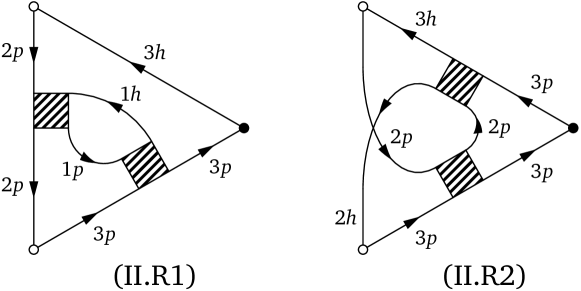
Figure 11: Dominant vertex corrections in the low-temperature low-density limit. The shaded boxes represent a particle-particle ladder series (pseudopotential). $1p$ and $1h$ stand for a particle or a hole in state $|1\rangle$, respectively, and similarly for the other states. The diagrams give a significant contribution only if the time ordering of the various vertices is such that all lines marked as particles go to the right (see Appendix C). The diagrams shown are right handed; there are two equivalent left-handed terms.

In the experimental setup of Ref. Fröhlich et al., 2012, the scattering length $a_{12}$ measuring the interaction $V_{12}$ between states $|1\rangle$ ($|F=9/2,m_{F}=-9/2\rangle$) and $|2\rangle$ ($|F=9/2,m_{F}=-7/2\rangle$) is close to a Feshbach resonance and was tuned on the attractive side from $0$ to $-300$, in units of the Bohr radius $a_{\text{B}}$. The interactions $V_{13}$ and $V_{23}$ between states $|1\rangle$ and $|3\rangle$ ($|F=9/2,m_{F}=-5/2\rangle$) and $|2\rangle$ and $|3\rangle$ are both nonresonant and repulsive and correspond to scattering lengths $a_{13}=+250a_{\text{B}}$ and $a_{23}=+130a_{\text{B}}$. In this configuration, we expect that the effect of $V_{13}$ is enhanced by the attractive $V_{12}$ in the correction (II.R1), while $V_{23}$ only contributes through the exchange process (II.R2). We speculate that most of the extra broadening observed in the measurements, with respect to the theory including $V_{12}$, but neglecting final-state interactions Fröhlich et al. (2012), is the result of these processes. A self-energy broadening due to the direct interaction between $|2\rangle$ and $|3\rangle$ in the initial state (accounted for in the type-I diagram of Fig. 3) is unlikely because such contributions require at least two holes in the final state and are suppressed by a factor $e^{-h\nu_{0}/k_{\text{B}}T}$ (see Appendix C). If the number of atoms excited in the final state is not too small, the self-energy in the final state associated with both $V_{13}$ and $V_{23}$ may also induce, in addition to energy shifts at lowest order, some broadening of type I, which enters the resolution function, as shown in Sec. IV.1. Explicit evaluations of the vertex corrections in Fig. 11 and of other self-energy effects are left for future works. It will be interesting to see whether and how these final-state effects change the line shape of the rf signal.

V Conclusion

We have presented a theoretical description of the rf spectroscopy of cold-atom systems, based on the second-order response theory at finite temperature. The difference between the usual golden-rule approach and this new description is that the latter focuses on the number $N_{f}$ of atoms transferred to the final state, while the former focuses on the transition rate $\dot{N}_{f}$. The second-order response approach accounts for the finite energy resolution implied by the envelope and the finite duration of the rf pulse and allows one to classify the various contributions using Feynman diagrams. The issue of inhomogeneity represents a challenge for the interpretation of rf experiments performed on interacting Fermi systems. Due to the density dependence of the self-energy, the rf line shape varies across the cloud. We have studied this effect at leading order in the density within the LDA and found that the static local Hartree shifts induce an apparent dispersion of the rf signal, similar to the dispersion expected in a homogeneous interacting Fermi gas from dynamical effects of higher order in the density. For three-dimensional gases with a Gaussian density profile, we have derived a simple expression for the momentum-integrated rf line shape, which takes into account the finite resolution and the inhomogeneous Hartree shifts.

Final-state effects are another challenge for rf experiments. We have considered the simplest of them, resulting either from a lifetime or from the interplay of inhomogeneity and Hartree shifts in the final state. More subtle final-state effects, such as those resulting from the spatial correlations between atoms, are described by vertex corrections. We have proposed a scheme to classify these terms and identified those which dominate at low temperature and low density. A numerical evaluation of the corresponding diagrams is needed to tell whether these effects change significantly the line shape of the rf signal.

Appendix A Analytic continuation of second-order response functions

In this appendix, we show that the second-order retarded susceptibility, defined in terms of the double commutator in Eq. (9), corresponds by analytical continuation to the imaginary-time correlator (11). We switch to a slightly lighter notation, set $\hbar=1$, and compute the second-order change of the expectation value of an observable $A$, in the presence of a perturbation $H^{\prime}=BF(t)$, where $B$ is an observable and $F(t)$ is a classical field. The second-order correction is

$$\langle A(t)\rangle^{(2)}=(-i)^{2}\int_{-\infty}^{t}dt_{1}\int_{-\infty}^{t_{1}}dt_{2}\\ \times\langle[[A(t),H^{\prime}(t_{1})],H^{\prime}(t_{2})]\rangle_{H}.$$ (54)

The ensemble average is taken over the eigenstates of the time-independent Hamiltonian $H$, such that invariance by translation in time applies: $\langle[[A(t),H^{\prime}(t_{1})],H^{\prime}(t_{2})]\rangle_{H}=\langle[[A(t-t_{1}),H^{\prime}(0)],H^{\prime}(t_{2}-t_{1})]\rangle_{H}$. Using this, and the expression of $H^{\prime}$, we can write

$$\langle A(t)\rangle^{(2)}=\int_{-\infty}^{\infty}dt_{1}dt_{2}\,\chi_{AB}^{(2)}(t-t_{1},t-t_{2})F(t_{1})F(t_{2}),$$ (55)

with the second-order susceptibility defined as

$$\chi_{AB}^{(2)}(t,t^{\prime})=(-i)^{2}\theta(t)\theta(t^{\prime}-t)\\ \times\langle[[A(t),B(0)],B(t-t^{\prime})]\rangle_{H}.$$ (56)

Introducing the Fourier transform of the various quantities in the integrand of Eq. (55) leads to the analogous of the second line in Eq. (9):

$$\langle A(t)\rangle^{(2)}=\int_{-\infty}^{\infty}\frac{d\omega}{2\pi}\frac{d\omega^{\prime}}{2\pi}\,e^{-i(\omega+\omega^{\prime})t}\\ \times\chi_{AB}^{(2)}(\omega,\omega^{\prime})F(\omega)F(\omega^{\prime}).$$ (57)

Out task is to show that

$$\chi_{AB}^{(2)}(\omega,\omega^{\prime})=\frac{1}{2}\mathscr{C}_{AB}^{(2)}(i\Omega\to\omega+i0^{+},i\Omega^{\prime}\to\omega^{\prime}+i0^{+}),$$ (58)

where $\mathscr{C}_{AB}^{(2)}(i\Omega,i\Omega^{\prime})$ is the Fourier transform of the imaginary-time correlator

$$\mathscr{C}_{AB}^{(2)}(\tau,\tau^{\prime})=\langle T_{\tau}A(\tau)B(0)B(\tau-\tau^{\prime})\rangle_{H}.$$ (59)

For this purpose, we show that the spectral representations of the functions $\chi_{AB}^{(2)}(\omega,\omega^{\prime})$ and $\frac{1}{2}\mathscr{C}_{AB}^{(2)}(i\Omega,i\Omega^{\prime})$ are identical.

Let us start with $\mathscr{C}_{AB}^{(2)}$. Splitting the imaginary-time integrals to take into account the time ordering, we have

$$\mathscr{C}_{AB}^{(2)}(i\Omega,i\Omega^{\prime})$$

$$\qquad=\int_{0}^{\beta}d\tau d\tau^{\prime}\,e^{i\Omega\tau}e^{i\Omega^{\prime}\tau^{\prime}}\mathscr{C}_{AB}^{(2)}(\tau,\tau^{\prime})$$

$$\qquad=\int_{0}^{\beta}d\tau\,e^{i\Omega\tau}\left[\int_{0}^{\tau}d\tau^{\prime}\,e^{i\Omega^{\prime}\tau^{\prime}}\langle A(\tau)B(\tau-\tau^{\prime})B(0)\rangle_{H}\right.$$

$$\quad\qquad\left.+\int_{\tau}^{\beta}d\tau^{\prime}\,e^{i\Omega^{\prime}\tau^{\prime}}\langle A(\tau)B(0)B(\tau-\tau^{\prime})\rangle_{H}\right].$$ (60)

To perform the time integrations, we introduce a complete set of eigenstates of $H$, $H|a\rangle=E_{a}|a\rangle$, we use the expression of the thermal average, $\langle(\cdots)\rangle=Z^{-1}\text{Tr}\,e^{-\beta H}(\cdots)$, we insert two times the identity $\openone=\sum_{a}|a\rangle\langle a|$, and we use the expression of the imaginary-time operators, e.g., $A(\tau)=e^{\tau H}Ae^{-\tau H}$. The averages in the square brackets of (A) become

$$\langle A(\tau)B(\tau-\tau^{\prime})B(0)\rangle_{H}$$

$$\qquad=\frac{1}{Z}\sum_{abc}\langle a|A|b\rangle\langle b|B|c\rangle\langle c|B|a\rangle e^{E_{a}(\tau-\beta)}e^{-E_{b}\tau^{\prime}}e^{E_{c}(\tau^{\prime}-\tau)}$$

$$\langle A(\tau)B(0)B(\tau-\tau^{\prime})\rangle_{H}$$

$$\qquad=\frac{1}{Z}\sum_{abc}\langle a|A|b\rangle\langle b|B|c\rangle\langle c|B|a\rangle e^{E_{a}(\tau^{\prime}-\beta)}e^{-E_{b}\tau}e^{E_{c}(\tau-\tau^{\prime})}.$$

The $\tau$ and $\tau^{\prime}$ integrations in (A) are now elementary and yield, after making use of the property $e^{i\Omega\beta}=e^{i\Omega^{\prime}\beta}=1$,

$$\mathscr{C}_{AB}^{(2)}(i\Omega,i\Omega^{\prime})=\frac{1}{Z}\sum_{abc}\langle a|A|b\rangle\langle b|B|c\rangle\langle c|B|a\rangle\\ \times\frac{1}{i\Omega+i\Omega^{\prime}+E_{a}-E_{b}}\left(\frac{e^{-\beta E_{a}}-e^{-\beta E_{c}}}{i\Omega+E_{a}-E_{c}}+\frac{e^{-\beta E_{b}}-e^{-\beta E_{c}}}{i\Omega-E_{b}+E_{c}}\right.\\ \left.+\frac{e^{-\beta E_{a}}-e^{-\beta E_{c}}}{i\Omega^{\prime}+E_{a}-E_{c}}+\frac{e^{-\beta E_{b}}-e^{-\beta E_{c}}}{i\Omega^{\prime}-E_{b}+E_{c}}\right).$$ (61)

A similar calculation leads to the spectral representation of the real-time susceptibility. We start from

$$\chi_{AB}^{(2)}(\omega,\omega^{\prime})=-\int_{-\infty}^{\infty}dtdt^{\prime}\,e^{i\omega t}e^{i\omega^{\prime}t^{\prime}}\theta(t)\theta(t^{\prime}-t)\\ \times\langle[[A(t),B(0)],B(t-t^{\prime})]\rangle_{H}.$$ (62)

The four terms of the double commutator are expressed as

$$\langle A(t)B(0)B(t-t^{\prime})\rangle_{H}$$

$$\qquad=\frac{1}{Z}\sum_{abc}\langle a|A|b\rangle\langle b|B|c\rangle\langle c|B|a\rangle e^{-\beta E_{a}}e^{iE_{a}t^{\prime}}e^{-iE_{b}t}e^{iE_{c}(t-t^{\prime})}$$

$$\langle B(t-t^{\prime})A(t)B(0)\rangle_{H}$$

$$\qquad=\frac{1}{Z}\sum_{abc}\langle a|A|b\rangle\langle b|B|c\rangle\langle c|B|a\rangle e^{-\beta E_{c}}e^{iE_{a}t^{\prime}}e^{-iE_{b}t}e^{iE_{c}(t-t^{\prime})}$$

$$\langle B(0)A(t)B(t-t^{\prime})\rangle_{H}$$

$$\qquad=\frac{1}{Z}\sum_{abc}\langle a|A|b\rangle\langle b|B|c\rangle\langle c|B|a\rangle e^{-\beta E_{c}}e^{iE_{a}t}e^{-iE_{b}t^{\prime}}e^{iE_{c}(t^{\prime}-t)}$$

$$\langle B(t-t^{\prime})B(0)A(t)\rangle_{H}$$

$$\qquad=\frac{1}{Z}\sum_{abc}\langle a|A|b\rangle\langle b|B|c\rangle\langle c|B|a\rangle e^{-\beta E_{b}}e^{iE_{a}t}e^{-iE_{b}t^{\prime}}e^{iE_{c}(t^{\prime}-t)}.$$

We perform the time integrations in (62) with the help of the identity

$$\int_{-\infty}^{\infty}dt\,e^{i\omega t}\theta(t)=\frac{i}{\omega+i0^{+}},$$

and obtain, using the notations $\omega^{+}=\omega+i0^{+}$ and ${\omega^{\prime}}^{+}=\omega^{\prime}+i0^{+}$,

$$\chi_{AB}^{(2)}(\omega,\omega^{\prime})=\frac{1}{Z}\sum_{abc}\langle a|A|b\rangle\langle b|B|c\rangle\langle c|B|a\rangle\\ \times\frac{1}{\omega^{+}+{\omega^{\prime}}^{+}+E_{a}-E_{b}}\left(\frac{e^{-\beta E_{a}}-e^{-\beta E_{c}}}{{\omega^{\prime}}^{+}+E_{a}-E_{c}}+\frac{e^{-\beta E_{b}}-e^{-\beta E_{c}}}{{\omega^{\prime}}^{+}-E_{b}+E_{c}}\right).$$

By exchanging the dummy variables $t_{1}$ and $t_{2}$ in the expression (55), we see that the susceptibility (56) can also be defined with the arguments $t$ and $t^{\prime}$ exchanged. We could therefore use an alternate definition of the susceptibility, which shows explicitly the symmetry under the exchange of the time arguments, e.g., $\frac{1}{2}[\chi^{(2)}_{AB}(t,t^{\prime})+\chi^{(2)}_{AB}(t^{\prime},t)]$ instead of Eq. (56). Exchanging the time arguments in Eq. (56) is equivalent to exchanging the two frequencies $\omega$ and $\omega^{\prime}$ in Eq. (62). After performing this symmetrization, we obtain the alternate definition of the susceptibility:

$$\chi_{AB}^{(2)}(\omega,\omega^{\prime})=\frac{1}{2}\frac{1}{Z}\sum_{abc}\langle a|A|b\rangle\langle b|B|c\rangle\langle c|B|a\rangle\\ \times\frac{1}{\omega^{+}+{\omega^{\prime}}^{+}+E_{a}-E_{b}}\left(\frac{e^{-\beta E_{a}}-e^{-\beta E_{c}}}{\omega^{+}+E_{a}-E_{c}}+\frac{e^{-\beta E_{b}}-e^{-\beta E_{c}}}{\omega^{+}-E_{b}+E_{c}}\right.\\ \left.+\frac{e^{-\beta E_{a}}-e^{-\beta E_{c}}}{{\omega^{\prime}}^{+}+E_{a}-E_{c}}+\frac{e^{-\beta E_{b}}-e^{-\beta E_{c}}}{{\omega^{\prime}}^{+}-E_{b}+E_{c}}\right).$$ (63)

Comparison of Eqs. (61) and (63) proves (58).

Appendix B Momentum density and density distribution

By inverting the analog of Eq. (38) for $n_{2}(\bm{r})$, one obtains an expression for $\mu-(1/2)m\omega_{r}^{2}r^{2}-(g/N_{0})n_{1}(\bm{r})$ as a function of $n_{2}(\bm{r})$. Inserting this expression into Eq. (39) gives

$$\langle n_{\bm{k}}\rangle_{\text{LDA}}=\int d^{d}r\,\frac{\mathscr{R}^{\text{(I${}^{\prime}$)}}\big{(}h\tilde{\nu}-(g/N_{0})n_{1}(\bm{r})\big{)}}{1-e^{\beta\varepsilon_{\bm{k}}}\Big{/}\text{Li}_{d/2}^{-1}\left[-\left(\frac{2\pi\hbar^{2}}{mk_{\text{B}}T}\right)^{d/2}n_{2}(\bm{r})\right]},$$

where $\text{Li}_{n}^{-1}$ is the inverse of the polylogarithm function. If $n_{1}(\bm{r})=n_{2}(\bm{r})\equiv n(\bm{r})$, the $\bm{r}$-dependence of the integrand stems from $n(\bm{r})$, and the spatial integration can be converted into a density integration, by introducing the density distribution $D(\mathfrak{n})=\int d^{d}r\,\delta\big{(}\mathfrak{n}-n(\bm{r})\big{)}$:

$$\langle n_{\bm{k}}\rangle_{\text{LDA}}=\int_{-\infty}^{\infty}d\mathfrak{n}\,\frac{D(\mathfrak{n})\mathscr{R}^{\text{(I${}^{\prime}$)}}\big{(}h\tilde{\nu}-(g/N_{0})\mathfrak{n}\big{)}}{1-e^{\beta\varepsilon_{\bm{k}}}\Big{/}\text{Li}_{d/2}^{-1}\left[-\left(\frac{2\pi\hbar^{2}}{mk_{\text{B}}T}\right)^{d/2}\mathfrak{n}\right]}.$$ (64)

For an ideal resolution, $\mathscr{R}^{\text{(I${}^{\prime}$)}}(\varepsilon)\propto\delta(\varepsilon)$, we have simply

$$\langle n_{\bm{k}}\rangle_{\text{LDA}}\propto\frac{D(h\tilde{\nu}N_{0}/g)}{1-e^{\beta\varepsilon_{\bm{k}}}\Big{/}\text{Li}_{d/2}^{-1}\left[-\left(\frac{2\pi\hbar^{2}}{mk_{\text{B}}T}\right)^{d/2}\frac{h\tilde{\nu}N_{0}}{g}\right]}.$$

This expression can be made more explicit in dimension $d=2$. On the one hand, $\text{Li}_{1}^{-1}(x)=1-e^{-x}$, and on the other hand, the density distribution can be evaluated explicitly. We have

$$D(\mathfrak{n})=\begin{cases}\displaystyle\frac{2\pi r_{0}}{|n^{\prime}(r_{0})|}&0\leqslant\mathfrak{n}\leqslant n(0)\vspace{2mm}\\ 0&\text{otherwise},\end{cases}$$

where $n^{\prime}(r)$ is the derivative of the radial density $n(r)$, $n(0)$ is the density at the trap center, and $n(r_{0})=\mathfrak{n}$. Differentiating Eq. (38) with respect to $r$, one finds

$$\frac{2\pi r}{|n^{\prime}(r)|}=\frac{2\pi}{m\omega_{r}^{2}N_{0}}\left[1+g+e^{-\frac{\mu-\frac{1}{2}m\omega_{r}^{2}r^{2}-(g/N_{0})n(r)}{k_{\text{B}}T}}\right].$$

The exponential in the square brackets can be expressed as a function of $n(r)$ only, by inverting Eq. (38) as above. For $r=r_{0}$, on thus gets

$$\frac{2\pi r_{0}}{|n^{\prime}(r_{0})|}=\frac{2\pi}{m\omega_{r}^{2}N_{0}}\left[1+g+b\left(\frac{\mathfrak{n}}{N_{0}}\right)\right],$$

where $b(\varepsilon)=1/(e^{\varepsilon/k_{\text{B}}T}-1)$. The resulting expression for the momentum distribution in two dimensions, and for an ideal resolution, is given in Eq. (40). Interestingly, the functional dependence of the density distribution on $\mathfrak{n}$, and consequently the dependence of the momentum distribution (40) on $\tilde{\nu}$, does not involve the total particle number $N_{1}$; only the cutoff depends on $N_{1}$ via $n(0)$.

Appendix C Classification of vertex corrections

The upper line in the diagram of type R in Fig. 2 corresponds to a hole in the final state $|3\rangle$, as implied by the ordering of the times, e.g., $\tau-\tau^{\prime}<\tau$. The lower line corresponds to a particle in the final state. Conversely, in the diagram of type L, the lower line corresponds to a hole ($0<\tau$) and the upper line to a particle. In both cases, the vertical line describes either a particle or a hole in the initial state $|2\rangle$, depending upon the ordering of the times $\tau-\tau^{\prime}$ and $0$. This is illustrated in Fig. 12 in the case of type-I diagrams. Each hole in the state $|3\rangle$ entails an occupation factor $f(\varepsilon_{3})\sim e^{-\beta h\nu_{0}}$, which is negligible if the thermal population of the final state is negligible. One such factor is canceled if—and only if—the time $\tau^{\prime}-\tau$ can reach the value $\beta$. (This applies to R diagrams; the same statement with $\tau^{\prime}-\tau$ replaced with $\tau-\tau^{\prime}$ applies to L diagrams.) The reason is as follows. The Green’s function for a free hole propagating between times $\tau_{1}$ and $\tau_{2}$ is $f(\varepsilon_{3})e^{-\varepsilon_{3}(\tau_{2}-\tau_{1})}$, whereas for a free particle it is $-f(-\varepsilon_{3})e^{-\varepsilon_{3}(\tau_{2}-\tau_{1})}$. All time dependencies from the various particle and hole lines in state $|3\rangle$ cancel, except at the two conversion vertices ($\circ$), leaving only the dependence $e^{-\varepsilon_{3}(\tau-\tau^{\prime})}$. Upon performing the time integrations as specified by Eq. (12), a factor $e^{\beta h\nu_{0}}$ is generated if the time $\tau^{\prime}-\tau$ ($\tau-\tau^{\prime}$ for L diagrams) is allowed to reach the value $\beta$. This explains the behaviors indicated in Fig. 12. In all cases, there is one hole in the final state ($3h$ line)—hence a factor $e^{-\beta h\nu_{0}}$—that is canceled for right-handed diagrams if $\tau-\tau^{\prime}<0$ and for left-handed ones if $\tau-\tau^{\prime}>0$. The two types of contributions were denoted (Ia) and (Ib) in Sec. II.3.

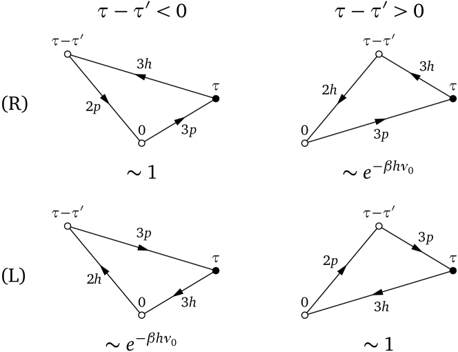
Figure 12: Contributions to the right-handed (R) and left-handed (L) diagrams of zeroth order in the interaction. The vertices are ordered horizontally by increasing imaginary time from left to right. $2p$ and $3p$ indicate particle lines in states $|2\rangle$ and $|3\rangle$, respectively, while $2h$ and $3h$ indicate hole lines.

Since the cancellation of the final-state hole occupation factor can only work once, we conclude that any diagram with more than one hole in the state $|3\rangle$ carries at least one factor $e^{-\beta h\nu_{0}}$ and is exponentially small if $k_{\text{B}}T\ll h\nu_{0}$. In particular, all corrections of the density vertex ($\bullet$) imply a connection between the lines $3p$ and $3h$ that cuts the $3h$ line and thus contains at least two holes in the final state. The first-order corrections of the conversion vertices ($\circ$) which survive in the limit $k_{\text{B}}T\ll h\nu_{0}$ are displayed in Fig. 13.

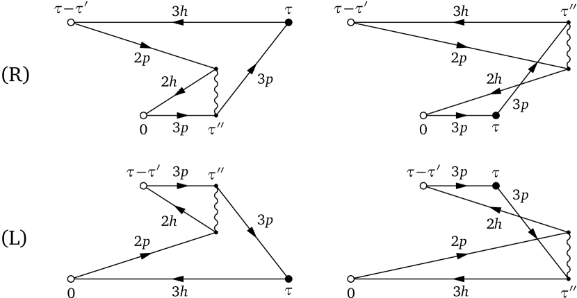
Figure 13: First-order right-handed (R) and left-handed (L) contributions to the $\circ$-vertex corrections, which survive in the limit $k_{\text{B}}T\ll h\nu_{0}$. The imaginary times $\tau-\tau^{\prime}$, $0$, $\tau^{\prime\prime}$, and $\tau$ are ordered horizontally as in Fig. 12. Any modification in the ordering of times produces at least one factor $e^{-\beta h\nu_{0}}$.

At higher orders in the interaction, we classify the vertex corrections like in the low-density expansion of the self-energy Galitskii (1958). A self-energy diagram containing $p$ hole lines, for instance a particle-hole ladder at order $p+1$, is proportional to $e^{p\beta\mu}$. Since $\mu\to-\infty$ as the density $n\to 0$ at any finite temperature, the contributions with one single hole dominate in this limit. These contributions are given by the particle-particle ladder series. Similarly, the vertex corrections with one single hole in either of the initial states $|1\rangle$ or $|2\rangle$ are expected to dominate at low density. Figure 11 shows the two contributions which we consider as the most important vertex corrections at low density. Both contain a single hole in the final state, and a single hole in one of the initial states. Any further decoration of these diagrams with interaction lines introduces new hole lines. The two right-handed first-order terms of Fig. 13 may be obtained from the diagram (II.R2) by removing one of the interaction boxes and evaluating at first order.

References

- Landau (1956) L. Landau, Zh. Eksp. Teor. Fiz. 30, 1058 (1956).
- Stewart (2001) G. R. Stewart, Rev. Mod. Phys. 73, 797 (2001).
- Schofield (1999) A. J. Schofield, Contemporary Physics 40, 95 (1999).
- Damascelli et al. (2003) A. Damascelli, Z. Hussain, and Z.-X. Shen, Rev. Mod. Phys. 75, 473 (2003).
- Vishik et al. (2010) I. M. Vishik, W. S. Lee, R.-H. He, M. Hashimoto, Z. Hussain, T. P. Devereaux, and Z.-X. Shen, New J. Phys. 12, 105008 (2010).
- Lu et al. (2012) D. Lu, I. M. Vishik, M. Yi, Y. Chen, R. G. Moore, and Z.-X. Shen, Annu. Rev. Cond. Mat. Phys. 3, 129 (2012).
- Allan et al. (2013) M. P. Allan, A. Tamai, E. Rozbicki, M. H. Fischer, J. Voss, P. D. C. King, W. Meevasana, S. Thirupathaiah, E. Rienks, J. Fink, D. A. Tennant, R. S. Perry, J. F. Mercure, M. A. Wang, J. Lee, C. J. Fennie, E.-A. Kim, M. J. Lawler, K. M. Shen, A. P. Mackenzie, Z.-X. Shen, and F. Baumberger, New J. Phys. 15, 063029 (2013).
- Törmä and Zoller (2000) P. Törmä and P. Zoller, Phys. Rev. Lett. 85, 487 (2000).
- Dao et al. (2007) T.-L. Dao, A. Georges, J. Dalibard, C. Salomon, and I. Carusotto, Phys. Rev. Lett. 98, 240402 (2007).
- Dao et al. (2009) T.-L. Dao, I. Carusotto, and A. Georges, Phys. Rev. A 80, 023627 (2009).
- Ketterle and Zwierlein (2008) W. Ketterle and M. Zwierlein, Riv. Nuovo Cimento Soc. Ital. Fis. 31, 247 (2008).
- Perali et al. (2008) A. Perali, P. Pieri, and G. C. Strinati, Phys. Rev. Lett. 100, 010402 (2008).
- Ohashi and Griffin (2005) Y. Ohashi and A. Griffin, Phys. Rev. A 72, 013601 (2005).
- He et al. (2005) Y. He, Q. Chen, and K. Levin, Phys. Rev. A 72, 011602 (2005).
- Shin et al. (2007) Y. Shin, C. H. Schunck, A. Schirotzek, and W. Ketterle, Phys. Rev. Lett. 99, 090403 (2007).
- Drake et al. (2012) T. E. Drake, Y. Sagi, R. Paudel, J. T. Stewart, J. P. Gaebler, and D. S. Jin, Phys. Rev. A 86, 031601 (2012).
- Sagi et al. (2012) Y. Sagi, T. E. Drake, R. Paudel, and D. S. Jin, Phys. Rev. Lett. 109, 220402 (2012).
- Yu and Baym (2006) Z. Yu and G. Baym, Phys. Rev. A 73, 063601 (2006).
- Baym et al. (2007) G. Baym, C. J. Pethick, Z. Yu, and M. W. Zwierlein, Phys. Rev. Lett. 99, 190407 (2007).
- Punk and Zwerger (2007) M. Punk and W. Zwerger, Phys. Rev. Lett. 99, 170404 (2007).
- Basu and Mueller (2008) S. Basu and E. J. Mueller, Phys. Rev. Lett. 101, 060405 (2008).
- Veillette et al. (2008) M. Veillette, E. G. Moon, A. Lamacraft, L. Radzihovsky, S. Sachdev, and D. E. Sheehy, Phys. Rev. A 78, 033614 (2008).
- Pieri et al. (2009) P. Pieri, A. Perali, and G. C. Strinati, Nat. Phys. 5, 736 (2009).
- He et al. (2009) Y. He, C.-C. Chien, Q. Chen, and K. Levin, Phys. Rev. Lett. 102, 020402 (2009).
- Fröhlich et al. (2012) B. Fröhlich, M. Feld, E. Vogt, M. Koschorreck, M. Köhl, C. Berthod, and T. Giamarchi, Phys. Rev. Lett. 109, 130403 (2012).
- Gupta et al. (2003) S. Gupta, Z. Hadzibabic, M. W. Zwierlein, C. A. Stan, K. Dieckmann, C. H. Schunck, E. G. M. van Kempen, B. J. Verhaar, and W. Ketterle, Science 300, 1723 (2003).
- Chin et al. (2010) C. Chin, R. Grimm, P. Julienne, and E. Tiesinga, Rev. Mod. Phys. 82, 1225 (2010).
- Schaich and Ashcroft (1971) W. L. Schaich and N. W. Ashcroft, Phys. Rev. B 3, 2452 (1971).
- Caroli et al. (1973) C. Caroli, D. Lederer-Rozenblatt, B. Roulet, and D. Saint-James, Phys. Rev. B 8, 4552 (1973).
- Chang and Langreth (1973) J.-J. Chang and D. C. Langreth, Phys. Rev. B 8, 4638 (1973).
- Keiter (1978) H. Keiter, Z. Phys. B Cond. Mat. 30, 167 (1978).
- Almbladh (2006) C.-O. Almbladh, J. Phys.: Conference Series 35, 127 (2006).
- Mahan (2000) G. D. Mahan, Many Particle Physics, 3rd ed. (Plenum, New York, 2000).
- Gaunt et al. (2013) A. L. Gaunt, T. F. Schmidutz, I. Gotlibovych, R. P. Smith, and Z. Hadzibabic, Phys. Rev. Lett. 110, 200406 (2013).
- Note (1) The self-consistent equation (38) breaks down for . In this regime of interaction, the negative pressure due to the Hartree term is stronger than the pressure due to Pauli exclusion, so that . In this case, the density profile implied by Eq. (38) has a minimum at the center of the trap.
- Galitskii (1958) V. M. Galitskii, Zh. Eksp. Teor. Fiz. 34, 151 (1958).