Effects of hidden nodes on network structure inference

Abstract

Effects of hidden nodes on inference quality of observed network structure are explored based on a disordered Ising model with hidden nodes. We first study analytically small systems consisting of a few nodes, and find that the magnitude of the effective coupling grows as the coupling strength from the hidden common input nodes increases, while the field strength of the input node has opposite effects. Insights gained from analytic results of small systems are confirmed in numerical simulations of large systems. We also find that the inference quality deteriorates as the number of hidden nodes increases. Furthermore, increasing field variance of hidden nodes improves the inference quality of the effective couplings, but worsens the quality for the effective fields. In addition, attenuated coupling strengths involved in at least one hidden node lead to high quality of coupling inference.

1 Introduction

Due to recent progresses in multi-electrode recording techniques in experimental neuroscience, the neural activity measurement of a population of increasing number of neurons becomes possible [1, 2], which provides a large opportunity and also a big challenge for the large-scale data analysis or dimensionality reduction [3], to understand how sensory processing, working memory or decision making arises from neural circuits. However, the brain region the current recording techniques can measure is very limited, therefore, the measured population of neurons is not completely isolated. Still there are many unobserved neurons outside this population (some may be upstream neurons), but interacting with neurons inside the observed population [4, 5, 6, 7]. The inferred interactions from the neural data are usually termed functional or effective connectivity, since the data fitting captures only part of the statistical features of the spike train data for algorithmic simplicity.

Recently, there appear intensive research interests on the inference problem of a random kinetic Ising model with hidden nodes [8, 9, 10, 11]. However, a systematic study of the effects of hidden nodes on the structure inference is still lacking based on widely used equilibrium models. Here, we explore these effects based on the maximal entropy model (also called the disordered Ising model) extensively used to model and fit the neural data in recent studies [12, 13, 14, 6]. We separate an unobserved part of network (a hidden subnetwork) from the full model, and probe the effects of hidden nodes first in small systems with a few nodes where the analytic study is available, then in large systems where we performed extensive numerical simulations under various settings. In fact, the correlation observed between two neurons may arise from a hidden common input outside the measured population. In addition, the interaction between two neurons may be mediated by a chain of unobserved neurons. How the unobserved part of the network affects the final inference quality will be the focus of this paper.

For a model study, the data used for inference are collected with high quality, such that the final result does not strongly depend on the inference method. In numerical simulations, we used the naive mean-field (nMF) method [15, 16, 17] to reconstruct the interaction strengths between neurons in the observed network. nMF relies simply on the inverse of the correlation matrix, which is also suitable for analytic studies of small systems with a few nodes. For small systems, we found that the effective field of observed neurons receiving a common input increases with the external field (firing bias) applied to the hidden input, while neurons interacting directly with the hidden input show different behavior from those that do not have a direct interaction. The effective couplings between neurons receiving a common input decreases with increasing firing bias of the hidden input. However, the neurons without a direct interaction (with the hidden input) seem to be unaffected in terms of their inferred coupling values. Furthermore, if two neurons are mediated by a chain of hidden neurons, the inferred interaction strength decreases with increasing chain length. Insights gained from the small size network are confirmed in numerical simulations of large size networks, from which, we showed that the inference performance deteriorates with increasing size of the unobserved network, and enhanced coupling strengthes between neurons in the unobserved part will increase the inference error for both the couplings and fields. Interestingly, if we increase the field strength of the unobserved neurons, the inference of couplings for the observed neurons will be improved, while the quality of the field inference still deteriorates.

The rest of this paper is organized as follows. The disordered Ising model compatible with the data is defined in Sec. 2. In Sec. 3, we present an analytic study on small systems. In Sec. 4, we present numerical simulation results on large systems. Conclusion is given in Sec. 5.

2 Disordered Ising model with hidden nodes

The experimental data can be described by $P$ independent sampled configurations $\{\boldsymbol{\sigma}^{\mu}\}(\mu=1,\ldots,P)$ where $\boldsymbol{\sigma}$ is an $N-$dimensional vector (the entry of the vector takes a binary value $\pm 1$) and $N$ is the network size. To build a minimal model to fit these data, one can take the constraints up to the second-order correlations in the data, resulting in the following maximal entropy model [18]:

$$P(\boldsymbol{\sigma})=\frac{1}{Z}\exp\left[\sum_{i<j}J_{ij}\sigma_{i}\sigma_{j}+\sum_{i}h_{i}\sigma_{i}\right].$$ (1)

The coupling terms $\{J_{ij}\}$ correspond to the correlation constraints ($\left<\sigma_{i}\sigma_{j}\right>_{P(\boldsymbol{\sigma})}=\left<\sigma_{i}\sigma_{j}\right>_{{\rm data}}$), while the field terms $\{h_{i}\}$ correspond to the magnetization constraints ($\left<\sigma_{i}\right>_{P(\boldsymbol{\sigma})}=\left<\sigma_{i}\right>_{{\rm data}}$). $Z$ is a normalization constant. The symmetric coupling may take either positive value or negative value, and the field also has the same situation, depending on the data [13, 6]. Hence, in general, we call this data-driven model a disordered Ising model or a spin glass model [19].

From Eq. (1), one can define an energy term $E=-\sum_{i<j}J_{ij}\sigma_{i}\sigma_{j}-\sum_{i}h_{i}\sigma_{i}$, then the distribution in Eq. (1) is known as a Boltzmann distribution in statistical mechanics [20]. In this paper, we divide the full network into observed (visible) part and unobserved (hidden) part, and study the effects of hidden part on the inference quality. We also assume the observed neurons have originally no firing biases. Therefore, the energy term becomes,

$$E=-\sum_{i<j}J_{ij}^{ab}\sigma_{i}^{a}\sigma_{j}^{b}-\sum_{i}h_{i}^{H}\sigma_{i}^{H},$$ (2)

where $a,b=V,H$, and $J_{ij}^{VV}$ $(J_{ij}^{HH})$ specifies the coupling strength between two neurons from the visible (hidden) part, and $J_{ij}^{VH}$ $(J_{ij}^{HV})$ indicates the coupling strength between two neurons one of which comes from the hidden part. All these coupling strengthes follow a Gaussian distribution with zero mean and variance $\sigma_{J}/c$. The field also follows a Gaussian distribution with zero mean and variance $\sigma_{h}$. In the simulation, one can also control the number of neurons in the hidden part, defined by $N_{h}$. In the full network, each neuron is connected to $c$ other neurons on average without self-interaction.

In general, it is quite difficult to infer the couplings or fields related to hidden nodes given the observed data [21, 15], although some special connection structure could be assumed for hidden part to make the inference possible at large network sizes [22, 23]. Here, we focus on the effects of hidden part on the inference quality of network structure of observed part. For simplicity, we used naive mean-field method to infer the couplings and fields in observed part and tested the inference performance against various control parameters. First, we define a connected correlation $C_{ij}=\left<\sigma_{i}\sigma_{j}\right>_{{\rm data}}-m_{i}m_{j}$, where the magnetization $m_{i}=\left<\sigma_{i}\right>_{\rm data}$. Then the coupling between neuron $i$ and neuron $j$ can be reconstructed by [15]

$$J_{ij}^{VV}=-(\mathbf{C}^{-1})_{ij}.$$ (3)

After the coupling is obtained, the field for neuron $i$ is inferred by [15]

$$h_{i}^{V}=\tanh^{-1}(m_{i})-\sum_{j\neq i}J_{ij}^{VV}m_{j}-m_{i}\left[\frac{1}{1-m_{i}^{2}}-(\mathbf{C}^{-1})_{ii}\right].$$ (4)

Eq. (3) is derived based on the mean-field equation $m_{i}=\tanh(\sum_{j\neq i}J_{ij}m_{j}+h_{i})$ and the linear-response theory $C_{ij}=\partial m_{i}/\partial h_{j}$ [15, 16]. A variety of advanced mean field approximations can be reduced to this simple approximation under certain conditions, e.g., high temperature or small correlation [17]. The last term in Eq. (4) is related to an effective self-coupling playing a key role in accurate field inference. However, a more natural and accurate way for field inference is applying an adaptive Onsager correction term [17]. For simplicity, we used the naive mean-field method in this paper.

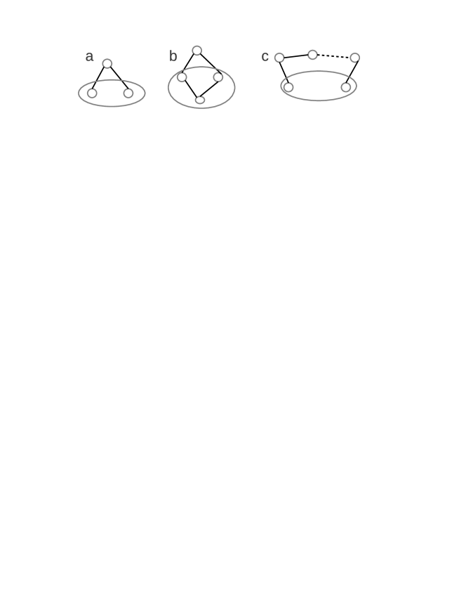
Figure 1: Small systems with hidden nodes. Neurons are indicated by gray circles, and the line indicates the direct interaction. The observed part is marked by an ellipse. Two neurons receiving a hidden common input (a). Three neurons with only two of them receiving a hidden common input (b). The interaction between two neurons mediated by a chain of unobserved neurons (c). The dashed line indicates the other $(L-3)$ unobserved neurons.

3 Small size system: analytic studies

In this section, we study analytically effects of hidden nodes on small size system, which could further provide insights towards understanding these effects on large systems.

3.1 Three-neuron system with one common hidden input

We first consider a three-neuron system with one common hidden input shown in Fig. 1 (a). We assume the observed neurons interact with the hidden neuron with the same coupling strength $J$, and the hidden neuron has a firing bias $h$. The normalization constant $Z_{a}=2\sum_{\sigma,\sigma^{\prime}}\cosh(J\sigma+J\sigma^{\prime}+h)$ where ${\sigma,\sigma^{\prime}}$ are states of the observed neurons. Therefore, the exact observed connected correlation ($C$) are given by:

$$C = 1-\frac{4\cosh h}{\cosh(2J+h)+\cosh(2J-h)+2\cosh h}-mm^{\prime},$$ (5)

$$m = m^{\prime}=\frac{\cosh(2J+h)-\cosh(2J-h)}{\cosh(2J+h)+\cosh(2J-h)+2\cosh h},$$ (6)

where $m(m^{\prime})$ is the observed magnetization. According to Eq. (3), the inferred coupling is given by:

$$J_{{\rm eff}}=\frac{C}{(1-m^{2})(1-m^{\prime 2})-C^{2}}.$$ (7)

The field can be predicted by:

$$h_{\rm eff}=h^{\prime}_{{\rm eff}}=\tanh^{-1}(m)-J_{{\rm eff}}m-m\left[\frac{1}{1-m^{2}}-\frac{1-m^{2}}{(1-m^{2})^{2}-C^{2}}\right].$$ (8)

If we increase the field $h$ to a very large value, then we can get the correlation difference $\Delta C=C(h=0)-C(h\rightarrow\infty)=m^{2}$ and the coupling difference $\Delta J_{\rm{eff}}=\frac{m^{2}}{1-m^{4}}$, where $m=\frac{\sinh 2J}{1+\cosh 2J}$. Therefore, both differences are positive, implying that increasing the field will lower down both the correlations and the inferred couplings.

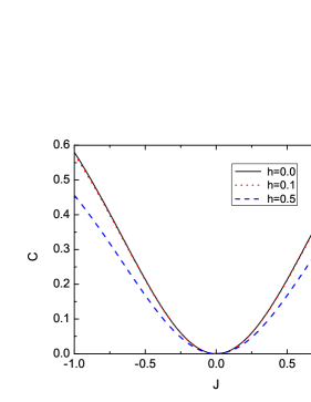
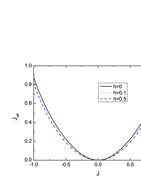
(a)   (b) (c)

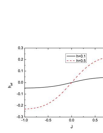
Figure 2: (Color online) Inference results corresponding to Fig. 1 (a). (a) connected correlation versus coupling strength between observed neurons and the hidden one. (b) effective coupling between observed neurons. Note that the true value is zero. (c) effective field for observed neurons. Note also that the true value is zero.

Results are shown in Fig. 2. As observed in Fig. 2 (a), increasing the external field of hidden input will lower down the connected correlation between two observed neurons. This effect also makes the predicted coupling between two observed neurons smaller than that in the presence of a smaller external field, as shown in Fig. 2 (b). However, the effective coupling increases as the absolute value of the coupling strength ($J^{VH}=J$) grows. Only when $J$ becomes very weak, $J_{\rm eff}$ gets close to zero which is the true value, due to the nature of the naive mean field approximation. The behavior of effective fields with $J$ and $h$ is shown in Fig. 2 (c). The external field of hidden input will increase the magnitude of the effective field applied on the observed neurons. For large $J$, the effective field seems to saturate to some large values but smaller than $h$. When $J$ changes its sign, so does $h_{{\rm eff}}$, which can be zero only when no hidden input interacts with the observed part.

3.2 Four-neuron system with one common hidden input

We consider one additional neuron in the observed part, but it doses not interact directly with the hidden neuron, as shown in Fig. 1 (b). We assume all $J^{VH}=J$, $J^{VV}=J$ except for the neurons interacting with the hidden neuron ($J_{12}^{VV}=0$). In the observed part, three neurons are given the indexes $1,2,3$. The hidden neuron has a firing bias $h$. In this case, $Z_{b}=4\cosh(2J)(\cosh(2J+h)+\cosh(2J-h))+8\cosh h$. The connected correlation between neuron $1$ and neuron $2$ is given by:

$$C = \frac{\cosh(2J)(\cosh(2J+h)+\cosh(2J-h))-2\cosh h}{\cosh(2J)(\cosh(2J+h)+\cosh(2J-h))+2\cosh h}-m_{1}m_{2},$$ (9)

$$m_{1} = m_{2}=\frac{\cosh(2J)(\cosh(2J+h)-\cosh(2J-h))}{\cosh(2J)(\cosh(2J+h)+\cosh(2J-h))+2\cosh h}.$$ (10)

$C_{13}$ and $C_{23}$ are given by:

$$C_{13}=C_{23}=\frac{\sinh(2J)(\cosh(2J+h)+\cosh(2J-h))}{\cosh(2J)(\cosh(2J+h)+\cosh(2J-h))+2\cosh h}-m_{1}m_{3},$$ (11)

$$m_{3}=\frac{\sinh(2J)(\cosh(2J+h)-\cosh(2J-h))}{\cosh(2J)(\cosh(2J+h)+\cosh(2J-h))+2\cosh h}.$$ (12)

Let $m_{1}=m_{2}=m$, $m_{3}=m^{\prime}$, $C_{13}=C_{23}=C^{\prime}$, we have the following inferred results:

$$J_{{\rm eff}} = \frac{C(1-m^{\prime 2})-C^{\prime 2}}{\Delta},$$ (13)

$$J_{{\rm in}} = \frac{C^{\prime}(1-m^{2}-C)}{\Delta},$$ (14)

where $J_{{\rm eff}}$ and $J_{{\rm in}}$ are inferred values of $J_{12}$ and $J_{23}(J_{13})$ respectively. $\Delta=(1-m^{2})((1-m^{2})(1-m^{\prime 2})-C^{\prime 2})-C(C(1-m^{\prime 2})-C^{\prime 2})+C^{\prime 2}(C-1+m^{2})$. It is easy to show that $C(h=0)-C(h\rightarrow\infty)=(\cosh^{2}(2J)-1)\cosh^{2}(2J)/(1+\cosh^{2}(2J))^{2}\geq 0$ and $|C^{\prime}(h=0)|-|C^{\prime}(h\rightarrow\infty)|=\cosh(2J)|\sinh(2J)|(\cosh^{2}(2J)-1)/(1+\cosh^{2}(2J))^{2}\geq 0$. One can also show that $J_{{\rm eff}}(h=0)-J_{{\rm eff}}(h\rightarrow\infty)=(\cosh^{4}(2J)-1)/(8\cosh^{2}(2J))\geq 0$ and $J_{{\rm in}}(h=0)=J_{{\rm in}}(h\rightarrow\infty)=(\cosh^{2}(2J)+1)\tanh(2J)/4$. These results can explain the interesting properties shown below. The fields are inferred as:

$$h_{{\rm eff}} = \tanh^{-1}(m)-J_{{\rm eff}}m-J_{{\rm in}}m^{\prime}-m\left[\frac{1}{1-m^{2}}-\frac{(1-m^{2})(1-m^{\prime 2})-C^{\prime 2}}{\Delta}\right],$$ (15)

$$h_{{\rm in}} = \tanh^{-1}(m^{\prime})-2J_{{\rm in}}m-m^{\prime}\left[\frac{1}{1-m^{\prime 2}}-\frac{(1-m^{2})^{2}-C^{2}}{\Delta}\right],$$ (16)

where $h_{{\rm eff}}$ and $h_{{\rm in}}$ are the inferred values of $h_{1}(h_{2})$ and $h_{3}$ respectively.

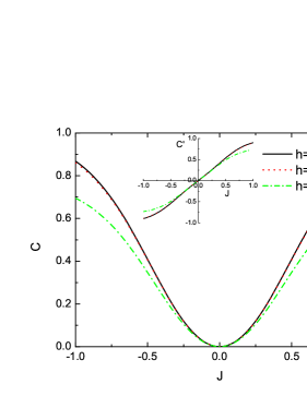
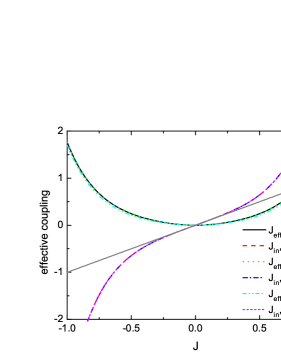
(a)   (b) (c)

Figure 3: (Color online) Inference results corresponding to Fig. 1 (b). (a) connected correlation versus coupling strength between observed neurons and the hidden one. The inset shows the connected correlation $C^{\prime}$ inside the observed network. (b) effective coupling between observed neurons. The gray line indicates equality. (c) effective field for observed neurons. Note that the true value is zero. The inset shows an enlarged view.

The connected correlation $C$ for neurons $1$ and $2$ is shown in Fig. 3 (a). Increasing the firing bias of the hidden neuron has the effect of lowering the connected correlation, which is already observed in a three-neuron system. This also occurs for $C^{\prime}$ (the inset). For effective coupling, the behavior becomes rich. First, the firing bias $h$ affects $J_{{\rm eff}}$ in a similar manner to that observed in Fig. 2 (b). However, it does not affect $J_{{\rm in}}$, and $J_{{\rm in}}$ is close to its true value only when the strength of $J$ is small ($|J|<0.22$). As observed in Fig. 3 (c), $h_{{\rm eff}}$ and $h_{{\rm in}}$ also show different behavior. The magnitude of $h_{{\rm in}}$ is much smaller than that of $h_{{\rm eff}}$, whereas, both of them grow with the firing bias $h$. There exists a range of $J$ where the inferred $h_{{\rm in}}$ takes a value close to zero. This range becomes narrow as $h$ increases. $h_{{\rm eff}}$ as a function of $J$ shows a behavior similar to that in the three-neuron system (see Fig. 2 (c)).

3.3 Two-neuron interaction mediated by a chain of hidden neurons

The interaction between two observed neurons can also be mediated by a chain of unobserved neurons which interact with each other by a coupling strength $J$ (see Fig. 1 (c)). Here we assume homogeneous interactions in the hidden part and no firing bias for hidden neurons, by focusing on how the effective coupling varies with the chain length $L$ and the coupling strength $J$. This chain will cause a correlation between observed neurons [20],

$$C=(\tanh J)^{L}.$$ (17)

And correspondingly, an effective coupling is given by

$$J_{{\rm eff}}=\frac{(\tanh J)^{L}}{1-(\tanh J)^{2L}}.$$ (18)

The effect of $J$ and $L$ is shown in Fig. 4. We find that the correlation becomes weak as $L$ increases, and the magnitude of the effective coupling also decreases with increasing $L$. $J_{{\rm eff}}$ is close to the true zero value only when $J$ falls within certain interval, otherwise, $|J_{{\rm eff}}|$ grows with $J$. This is consistent with the small correlation assumption made in the naive mean field approximation [15, 16].

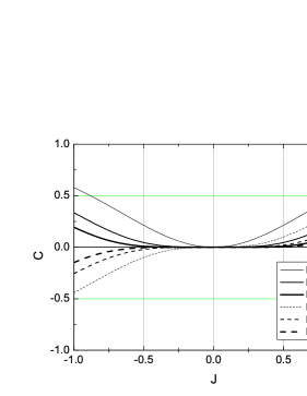
(a)      (b)

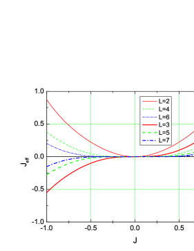
Figure 4: (Color online) Inference results corresponding to Fig. 1 (c). (a) connected correlation versus coupling strength in the hidden part. (b) effective coupling between observed neurons. $L$ is the chain length.

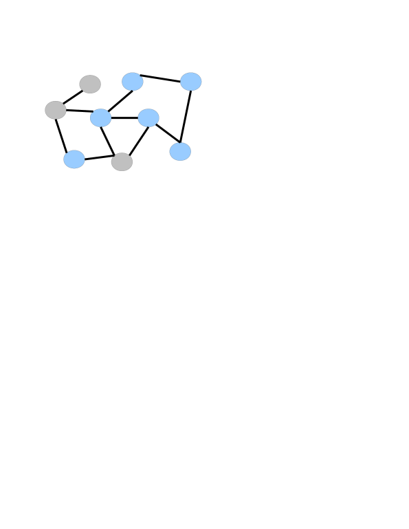
(a)      (b)

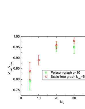
Figure 5: (Color online) (a) Network structure for large size system study. We show an example of $(N,N_{h})=(9,3)$. The gray circles indicate the hidden nodes while the others are visible nodes. In our simulations, we used $N=100$ with increasing value of $N_{h}$. Nodes are sparsely connected with either Poisson or power-law degree distribution. The set of hidden nodes is randomly selected for each network instance. (b) The ratio between the maximal degree of hidden nodes and that of all nodes. The random Poisson graph has mean degree $c$ and the random scale-free graph is characterized by the degree distribution $P(k)\propto k^{-\gamma}(k\geq k_{{\rm min}})$. The result is averaged over ten random instances.

4 Large size system: numerical simulations

For large size system, it is very difficult to perform an analytic calculation. However, the main effects of hidden nodes on the inference quality can be probed by numerical simulations. Here, we consider a system of size $N=100$, and the mean connectivity of each node $c=10$ unless otherwise specifically stated. Fig. 5 shows the network structure we consider. We consider the model defined on random Poisson graphs [24] first, and random scale-free graphs [25] at the end of this section. As the number of hidden nodes grows, the nodes of high connectivity (hubs) appear with higher probability in the hidden part (see Fig. 5 (b)). These hubs may play an important role in affecting the inference quality of the observed part.

The state space of the model is sampled by a standard Monte-Carlo procedure, which consists of an asynchronous update of all neurons at an elementary time step ($N$ proposed neuron’s state flips), i.e., the state of neuron $i$, say $\sigma_{i}$ is updated by

$$Prob(\sigma_{i}\rightarrow-\sigma_{i})=\exp\left(-2\sigma_{i}H_{i}\right),$$ (19)

where $H_{i}=h_{i}+\sum_{j\neq i}J_{ij}\sigma_{j}$, and the update goes over all $i$. The experimental data is collected as $P=10^{5}$ independent configurations (the inference will become more accurate with larger $P$ [26]); each of them was sampled with an interval equal to $40$ elementary time steps after sufficient thermal equilibration. These data are used to compute correlations and magnetizations. The inference quality is evaluated by the (relative) root-mean-square errors:

$$\delta_{J} = \left[\frac{\sum_{i<j}(J_{ij}^{VV}-\tilde{J}_{ij}^{VV})^{2}}{\sum_{i<j}(\tilde{J}_{ij}^{VV})^{2}}\right]^{1/2},$$ (20)

$$\Delta h = \left[\frac{\sum_{i}(h_{i}^{V}-\tilde{h}_{i}^{V})^{2}}{N-N_{h}}\right]^{1/2}.$$ (21)

$\tilde{J}_{ij}^{VV}$($\tilde{h}_{i}^{V}$) represents the true value. The reported results are the average over ten random realizations of the network, with the error bars showing the standard deviation.

4.1 Inference performance on random Poisson graph

4.1.1 Inference performance with increasing coupling variance

Fig. 6 reports results on networks with $h_{i}^{H}=0$ for any hidden neuron $i$. Increasing the number of unobserved neurons, one observes that the inference error $\delta_{J}$ also increases. One possible reason is, the growing unobserved part yields larger and larger correlations among observed neurons, resembling a glassy effect caused by increasing the coupling variance [17]. These correlations may contain higher-order ones. The overall effect is to cause some predicted couplings deviate strongly from their true values. The error increases with $\sigma_{J}$ as well, which is consistent with findings obtained in small systems (see Fig. 2 (b) and Fig. 3 (b)).

As shown in Fig. 7, by increasing $c$ but maintaining the same value of $\sigma_{J}/c$ , one should observe a larger effect of the hidden nodes, since this will increase the probability for a hidden node to have an interaction with the observed nodes. However, if only $\sigma_{J}$ is fixed, the error will decrease with $c$ because the overall strength of coupling is weakened.

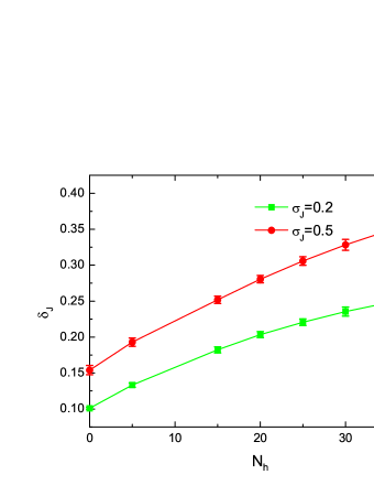
Figure 6: (Color online) Inference performance on random Poisson graphs ($c=10$) without firing biases for hidden neurons.

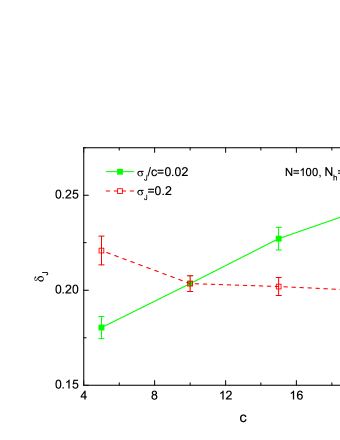
Figure 7: (Color online) Inference performance on random Poisson graphs versus $c$ without firing biases for hidden neurons.

4.1.2 Inference performance with increasing field variance of hidden nodes

To explore the effect of the field strength of hidden nodes, one can keep a small coupling variance while increasing the value of $\sigma_{h}$. Interestingly, the coupling error decreases as $\sigma_{h}$ increases, which becomes more apparent when $N_{h}$ gets larger, as shown in Fig. 8 (a). This result is consistent with that observed in Fig. 2 (b) and Fig. 3 (b). This can be explained by the fact that, increasing the number of unobserved neurons will make more observed neurons interact directly with the hidden ones, while the effective couplings between these observed neurons are expected to give a large contribution to the inference error. In particular, increasing field strength of hidden nodes results in smaller correlations, and thus the coupling prediction can be improved. This point can be easily understood from the analytic study of small systems, as shown in Fig. 2 (a) and Fig. 3 (a). Compatible with this effect, we also show the global mean correlation defined as $\bar{C}=\left[\frac{1}{|\mathcal{P}_{\rm obs}|}\sum_{(i,j)\in\mathcal{P}_{\rm obs}}C_{ij}^{2}\right]^{1/2}$ where $\mathcal{P}_{\rm obs}$ denotes the pair set of observed nodes, in the inset of Fig. 8 (a). We see clearly the global correlation decreases as the field variance increases.

In contrast to the coupling error, the field error still grows with the field variance, which becomes more evident at larger $N_{h}$, as shown in Fig. 8 (b). This may be related to the fact that, the effective fields of observed neurons interacting directly with the hidden neurons yield a larger contribution to the inference error, compared to those inside the observed part (not on the boundary between observed and unobserved part). The effective fields of the boundary neurons seem to be very sensitive to changes of firing biases of hidden neurons, as observed in Fig. 2 (c) and Fig. 3 (c).

As shown in Fig. 8 (c), in the presence of hidden nodes, the inferred coupling values over-estimate the true large positive couplings, while the large (in absolute value) negative couplings are slightly under-estimated, which was also observed in similar works [27, 28]. As $N_{h}$ varies, the inference error is mainly caused by non-existent connections and those connections with weak couplings.

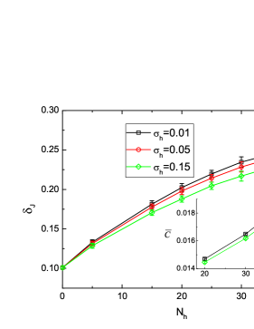
(a)      (b)
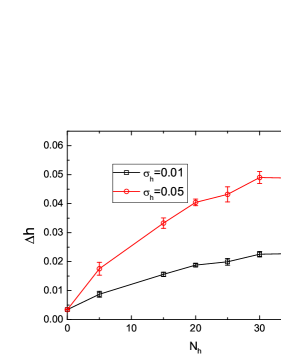
(c)

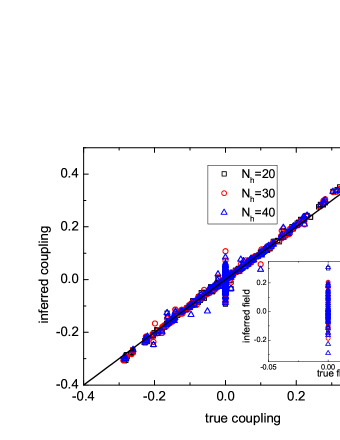
Figure 8: (Color online) Inference performance on random Poisson graphs ($c=10$) with $\sigma_{J}=0.2$. (a) Inference error for couplings versus the number of hidden neurons. The inset gives the global correlation versus the number of hidden neurons (the error bars are smaller than the symbol size). (b) Inference error for fields versus the number of hidden neurons. (c) The scatter plot comparing inferred couplings with the true ones for a typical example with $\sigma_{h}=0.15$. The line indicates equality. The inset shows the scatter plot for fields.

4.1.3 Inference performance with re-scaled couplings

Keeping a low value of $\sigma_{h}$, one can also explore the effect of coupling strength among hidden neurons or between hidden and visible neurons, by re-scaling the couplings, i.e., all $J^{VH}$ and $J^{HH}$ (hidden couplings) are enhanced by a factor $J\rightarrow gJ$ or attenuated as $J\rightarrow J/g$, where we choose $g=2$. Results are reported in Fig. 9. This case corresponds to adding a large perturbation to the couplings related to the hidden neurons, with the consequence that both the coupling and the field error increase when hidden couplings are enhanced. This finding is also consistent with the results reported in small systems (see Fig. 2 and Fig. 3).

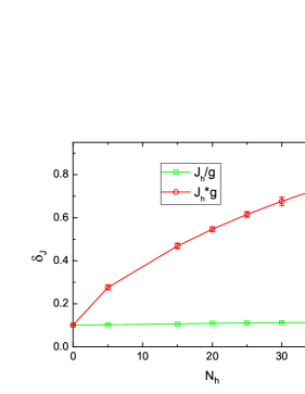
(a)      (b)

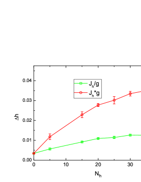
Figure 9: (Color online) Inference performance on random Poisson graphs ($c=10$) with $\sigma_{J}=0.2$ and $\sigma_{h}=0.01$. The interaction involved in at least one of the hidden neurons is enhanced by a factor $g=2$ or attenuated by a factor $1/g$. (a) inference error for couplings versus the number of hidden neurons. (b) inference error for fields versus the number of hidden neurons.

4.2 Inference performance on random scale-free graph

In this section, we study the effects of hidden nodes on random scale-free graph. Here the coupling strength follows the binary distribution $p(J)=\eta\delta(J-J_{0})+(1-\eta)\delta(J+J_{0})$ and the field is kept constant ($h=h_{0}$). In this case, $\eta=1.0$ corresponds to the ferromagnetic model while $\eta=0.0$ corresponds to the anti-ferromagnetic model. The behavior Fig. 10 (a) shows is similar to that observed in Fig. 6 and Fig. 8. Note that when $N_{h}$ becomes small, the relative error $\delta_{J}$ shows larger value at smaller $J_{0}$. This is because the overall strength of the denominator in the definition of $\delta_{J}$ dominates the error when $N_{h}$ is small, and does not mean that the inference quality at the large $J_{0}$ is better than that at the small $J_{0}$ (see Fig. 10 (b) for the scatter plots of a typical example). Fig. 10 (c) shows the inference performance of ferromagnetic and anti-ferromagnetic models, implying that the inference quality of either coupling or field deteriorates as the number of hidden nodes increases.

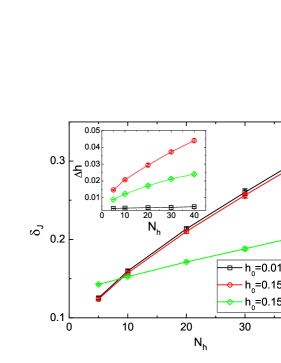
(a)      (b)
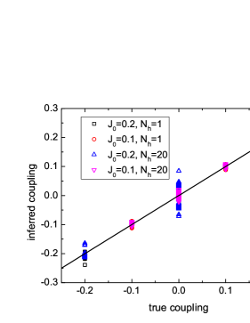
(c)

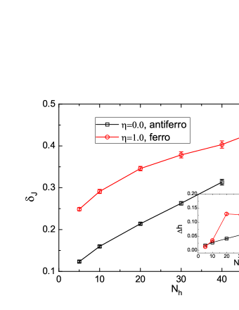
Figure 10: (Color online) Inference performance on random scale-free graph ($k_{{\rm min}}=5,\gamma=3$). (a) Inference error versus the number of hidden neurons with $\eta=0.5$. (b) The scatter plot for a typical example with $\eta=0.5$ and $h_{0}=0.15$. The line indicates equality. (c) Inference error for ferromagnetic and anti-ferromagnetic model with $J_{0}=0.2$ and $h_{0}=0.15$.

5 Conclusion

In this work, we study effects of unobserved part of a network on the inference quality of network structure of the observed part. We first study analytically the small size network with a few neurons, and find that, the effective couplings between the boundary neurons decreases as the firing bias of the hidden common input neuron increases, whereas, this firing bias does not affect the effective couplings inside the observed network. These effective couplings grow as the magnitude of the input coupling strengthes increases. Increasing firing bias of the hidden input will also increase the effective field of the boundary neurons which show different behavior from those neurons inside the observed part.

All these interesting properties are also observed in numerical simulations of large networks. The inference quality for both couplings and fields deteriorates as the size of the unobserved part grows, which can be explained by the fact that an increasing number of hidden neurons causes higher-order correlations in the observed data and furthermore a larger deviation of the inferred coupling from its true value, mimicking a glassy phase arising in observed networks. Interestingly, increasing field variance of hidden neurons improves the inference quality of the effective couplings, but worsens the quality for the effective fields. In addition, attenuated coupling strengthes involved in at least one hidden neuron lead to high quality of coupling inference. Our work demonstrates the hidden part in a full network does have a significant influence on the inference quality of the observed network structure (for both Poisson graph and scale-free graph), showing many interesting properties, as revealed in both small networks and large networks.

As new advanced experimental recording techniques are proposed, the number of measured neurons becomes larger and larger, providing greater challenges for large-scale neural data analysis. The effects of hidden neurons on the inference quality, based on a toy model study in this paper, provide insights towards understanding the interaction between observed part and unobserved part in terms of network structure prediction. Another interesting extension of the current work is to consider the Potts model which is widely used in protein structure prediction [29] (and references therein).

References

References

- [1] O. Marre, D. Amodei, N. Deshmukh, K. Sadeghi, F. Soo, T. E. Holy, and M. J. Berry. J. Neurosci., 32:14859–14873, 2012.
- [2] A. Berényi, Z. Somogyvari, A. J. Nagy, L. Roux, J. D. Long, S. Fujisawa, E. Stark, A. Leonardo, T. D. Harris, and G. Buzsaki. J. Neurophysiol, 111:1132–1149, 2014.
- [3] J. P. Cunningham and B. M. Yu. Nat. Neurosci., 17:1500–1509, 2014.
- [4] P. K. Trong and F. Rieke. Nat. Neurosci., 11:1343–1351, 2008.
- [5] J. Hertz, Y. Roudi, and J. Tyrcha. e-print arXiv:1106.1752, 2011.
- [6] G. Tkacik, O. Marre, D. Amodei, E. Schneidman, W. Bialek, and M. J. Berry II. PLoS Comput Biol, 10:e1003408, 2014.
- [7] S. Keshri, E. Pnevmatikakis, A. Pakman, B. Shababo, and L. Paninski. e-print arXiv:1309.3724, 2013.
- [8] Nir Friedman, Kevin Murphy, and Stuart Russell. In Proceedings of the Fourteenth Conference on Uncertainty in Artificial Intelligence, UAI’98, pages 139–147, San Francisco, CA, USA, 1998. Morgan Kaufmann Publishers Inc.
- [9] B. Dunn and Y. Roudi. Phys. Rev. E, 87:022127, 2013.
- [10] J. Tyrcha and J. Hertz. Mathematical Biosciences and Engineering, 11:149–165, 2014.
- [11] L. Bachschmid-Romano and M. Opper. J. Stat. Mech.: Theory Exp, 2014(6):P06013, 2014.
- [12] E. Schneidman, M. J. Berry, R. Segev, and W. Bialek. Nature, 440:1007, 2006.
- [13] H. Huang and H. Zhou. Phys. Rev. E, 85:026118, 2012.
- [14] J. Barton and S. Cocco. J. Stat. Mech.: Theory Exp, page P03002, 2013.
- [15] H. J. Kappen and F. B. Rodriguez. Neural Comput, 10:1137, 1998.
- [16] T. Tanaka. Phys. Rev. E, 58:2302, 1998.
- [17] H. Huang and Y. Kabashima. Phys. Rev. E, 87:062129, 2013.
- [18] E. T. Jaynes. Phys. Rev., 106:620–630, 1957.
- [19] M. Mézard, G. Parisi, and M. A. Virasoro. Spin Glass Theory and Beyond. World Scientific, Singapore, 1987.
- [20] J. M. Yeomans. Statistical Mechanics of Phase Transitions. Oxford University Press, Oxford, 1992.
- [21] D. H. Ackley, G. E. Hinton, and T. J. Sejnowski. Cognitive Science, 9:147, 1985.
- [22] Lawrence K. Saul, Tommi Jaakkola, and Michael I. Jordan. Journal of Artificial Intelligence Research, 4:61–76, 1996.
- [23] G Hinton, S Osindero, and Y Teh. Neural Computation, 18:1527–1554, 2006.
- [24] M. Mézard and G. Parisi. EPL (Europhysics Letters), 3:1067, 1987.
- [25] D.-H. Kim, G. J. Rodgers, B. Kahng, and D. Kim. Phys. Rev. E, 71:056115, 2005.
- [26] V. Sessak and R. Monasson. J. Phys. A, 42:055001, 2009.
- [27] Yasser Roudi, Joanna Tyrcha, and John Hertz. Phys. Rev. E, 79:051915, 2009.
- [28] Timothy R. Lezon, Jayanth R. Banavar, Marek Cieplak, Amos Maritan, and Nina V. Fedoroff. Proceedings of the National Academy of Sciences of the United States of America, 103:19033–19038, 2006.
- [29] J. P. Barton, S. Cocco, E. De Leonardis, and R. Monasson. Phys. Rev. E, 90:012132, 2014.