Tunneling time calculations for general finite wavepackets based on the presence time formalism

Abstract

We analyze the tunneling time problem via the presence time formalism. With this method we reproduce previous results for very long wavepackets and we are able to calculate the tunneling time for general wavepackets of arbitrary shape and length. The tunneling time for a general wavepacket is equal to the average over the energy components of the standard phase time. With this approach we can also calculate the time uncertainty. We have checked that the results obtained with this approach agree extremely well with numerical simulations of the wavepacket evolution.

I Introduction

The time spent by a particle in a given region of space is a problem that has been approached from many different points of view. There exits a huge literature on the tunneling phenomena for electrons through a barrier. Landauer and Martin LM94 pointed out that there is no clear consensus about simple expressions for time in quantum mechanics (QM), where there is not a Hermitian operator associated with it. Hartman HM62 asserted that for opaque barriers the tunneling time is independent of the barrier length and the time spent by the particle in these regions can be less than the time required to travel the same distance in vacuum. However, many physicists hesitated to deal with Hartman s results since a very fast tunneling implies that the tunneling velocity or the average velocity may become higher than the vacuum light velocity $c$. One can define the traversal time as the time during which a transmitted particle interacts with the region of interest measured by some physical clock which can detect the particle’s presence after leaving the region. For electrons, this approach can utilize the Larmor precession frequency of the spin produced by a weak magnetic field acting within the barrier region BZ671 ; BZ672 ; BT83 . Analogously, our group GO95 proposed a clock based on the Faraday effect to measure the interaction time for electromagnetic waves in a slab or a periodic structure. Another approach consists of calculating the traversal time of a particle through a barrier by following the behavior of a wavepacket and determining the delay due to the structure of the region. In this approach an emerging peak is not necessarily related to the incident peak in a causative way LAN93 . The phase time is the time which elapses between the peak of the wavepacket entering the barrier and leaving it and can be defined as the energy derivative of the phase.

Often, more than one tunneling time are involved in the problem. One can define a time $\tau_{y}$ associated with the direction of propagation and another time $\tau_{z}$ related to the transverse direction. B ttiker BT83 assumed that the relevant interaction time $\tau^{\rm BL}$ depends on both characteristic times and is given by

$$\tau^{\rm BL}=\sqrt{\tau_{y}^{2}+\tau_{z}^{2}},$$ (1)

which is the so called Büttiker–Landauer time for transmitted particles. Gasparian et al. GP93 ; GOR95 introduced a method based on Green’s functions and obtained a complex tunneling time, $\tau$. The real and imaginary part of this complex time were related to $\tau_{z}$ and $\tau_{y}$, respectively.

Other method to calculate the traversal time uses the Feynman path-integral approach of QM. Sokolovski and Baskin SB87 applied this formulation to obtain a traversal time. Sokolovski and Connor SC90 studied the tunneling time for wavepackets via this path-integral approach. For the square potential barrier, Fertig FT90 , using the path decomposition of Auerbach and Kivelson AK85 , defined a propagator that corresponds to the amplitude for tunneling between two points on opposite sides of the barrier with initial energy $E$, summed over the Feynman paths that spend a time $\tau$ inside the barrier.

In QM we can only measure quantities for which we have introduced a Hermitian operator. For these quantities, expectation values can be calculated and checked experimentally. However, time appears in the standard quantum-mechanical approach only as a parameter and therefore its expectation value is not defined. Moreover, Pauli PAU58 argued that a self-adjoint time operator implies an unbounded energy spectrum. In spite of this, many authors have proposed time operators and others have developed formalisms for arrival times in QM (for a review see Muga et al. MU00 ). Allcock ALL69 was the first to focus on the concept of arrival time, rather than on time operators, and concluded that wave mechanics cannot give an exact and ideal definition of arrival time. Werner WER86 overcame Pauli’s theorem by introducing non-self-adjoint operators in the framework of positive operator valued measures (POVMs). León et al. LE00 introduced a formalism for the calculation of the time of arrival for particles travelling through a region with a given potential energy. They employed quantum canonical transformations from the free to the interacting cases to compute the time of arrival in the context of the POVMs. However, it has been criticized that this approach does not always recover the classical expression for the arrival time when the effects of non-commutativity of the operators involved may be neglected BE01 .

Many authors have developed formalisms based on time operators rather than arrival times in QM OR74 ; RE77 ; KO94 ; KO01 . In these approaches, the average presence time at position $y$ for a spatial wavepacket $\Psi(y,t)$ is defined as

$$\langle t(y)\rangle\equiv\frac{\int_{-\infty}^{+\infty}\mathrm{d}t|\Psi(y,t)|^{2}\ t}{\int_{-\infty}^{+\infty}\mathrm{d}t|\Psi(y,t)|^{2}},$$ (2)

provided that this integral exists. Kobe et al.KO94 named the time operator whose average is given by Eq. (2) as the ”tempus” operator, and one can study efficiently the tunneling time through a barrier via the local value of this operator KO01 .

We studied numerically the tunneling time for electronic wavepackets in nanostructures and found that the finite size effect of the incident wavepacket was relevant when treating tunneling time in this spatial scale GO04 . The aim of this work is to show first that the approach based on the presence time gives equivalent results to standard treatments for very long wavepackets. In second place, we want to study finite size effects of the wavepacket in the tunneling time with this formalism, which is specially suited for this problem. We also want to compare the results obtained with the presence time formalism with those obtained using the time of arrival approach of León et al. LE00 .

The plan of the work is as follows. In Sec. II we introduce the presence time formalism and apply this method to the simplest case of free propagation. In Secs. III and IV we calculate, within the framework of the presence time formalism, the tunneling time and its uncertainty for a wavepacket which moves towards a rectangular barrier, respectively. In Sec. V we present some numerical results which include the finite size effect of the electronic wavepacket in the tunneling time and its uncertainty for a rectangular potential barrier. We also calculate the traversal time and its uncertainty for photons crossing a set of layers with a frequency gap. Finally, we summarize our results in Sec. VI.

II Presence time formalism

The calculation of the average presence time can be performed in terms of integrals over the energy, instead of integrals over time as in Eq. (2). To this aim, it is convenient to consider only scattering states incident with positive momenta so that there is no energy degeneracy. Then we can define the energy wavepacket in the following way

$$\Phi(y,E)=(2\pi\hbar)^{-1/2}\int_{-\infty}^{\infty}dt\ \Psi(y,t)\ \exp[i(Et)/\hbar],$$ (3)

where $\Psi(y,t)$ is the physical wavepacket in the space representation. We can write the average presence time, Eq. (2), as a expectation value of the energy derivative operator $-i\hbar\partial_{E}$ in the energy representation EGUS00

$$\langle t(y)\rangle=\frac{1}{P}\int_{0}^{\infty}\mathrm{d}E\ \Phi^{\ast}(y,E)\left[-i\hbar\left(\partial\over\partial E\right)\right]\Phi(y,E),$$ (4)

where $P$ is the normalization factor

$$P(y)=\int_{0}^{\infty}\mathrm{d}E\ |\Phi(y,E)|^{2}.$$ (5)

We will asume that the energy wavefunctions $\Phi(y,E)$ are continuous, differentiable and square integrable in the energy variable. If we further restrict to functions satisfying $\Phi(y,E=0)=0$ then the energy derivative operator $-i\hbar\partial_{E}$ is Hermitian OR74 . For shortness, we will refer to this operator as $\widehat{T}$ from now on.

To illustrate the presence time formalism, we consider first a wavepacket propagating in free space. At $t=0$ this wavepacket is peaked at $y_{0}$, has an spatial width $\Delta y$ and moves to the right. The components of the wavepacket in the energy representation are

$$\Phi(y,E)=G(E)\ \exp\left[i\ k(y-y_{0})\right],$$ (6)

where $G(E)$ is a normalized weight peaked at $E_{0}$ with an energy width $\Delta E$, and $k(E)=\sqrt{2mE}/\hbar$ is the corresponding wavenumber. Substituting expression (6) in Eq. (4) we obtain for the expectation value of $\widehat{T}$ at a point $y$

$$\langle\widehat{T}(y)\rangle=\frac{1}{P}\ \int_{0}^{\infty}\mathrm{d}E\ G^{2}(E)\ \left[\tau_{\rm cl}(y,E)-i\ \tau_{\rm G}(E)\right],$$ (7)

where $\tau_{\rm cl}(y,E)$ is the time it takes the particle to travel from $y_{0}$ to $y$ with velocity $\sqrt{2mE}/m$

$$\tau_{\rm cl}(y,E)=\frac{m\ (y-y_{0})}{\sqrt{2mE}},$$ (8)

and $\tau_{\rm G}$ is the partial derivative of the natural logarithm of the weight $G(E)$ with respect to the energy,

$$\tau_{\rm{G}}(E)=\hbar\ {\partial\ln G(E)\over\partial E}.$$ (9)

The real part of the time is the average of the classical time at $y$ for a particle with energy $E$ weighted by the probability density in the energy representation.

We can easily prove the hermiticity of $\widehat{T}$ in this case by showing that the imaginary part of $\langle\widehat{T}\rangle$ cancels. Introducing Eq. (9) into Eq. (7) we can write the imaginary part of the expectation value of $\widehat{T}$ in the following way

$$\mathrm{Im}\left[\langle\widehat{T}(y)\rangle\right]=\int_{0}^{\infty}\mathrm{d}E\ G(E)\ {\partial G(E)\over\partial E}=\int_{a}^{b}\mathrm{d}G\ G=\left[\frac{G^{2}}{2}\right]_{a}^{b}=0,$$ (10)

where we have assumed that $G(E)$ tends asymptotically to $0$ in the energy limits.

Let’s calculate the uncertainty of $\widehat{T}$ for the free case. The expectation value of the square of $\widehat{T}$ is equal to

$$\langle\widehat{T}^{2}(y)\rangle=\int_{0}^{\infty}\mathrm{d}E\ G^{2}(E)\ \{[\tau_{\rm cl}^{2}(y,E)-\widetilde{\tau}_{\rm G}(E)-\tau_{\rm G}^{2}(E)],$$ (11)

where $\widetilde{\tau}_{\rm G}$ is the energy derivative of $\hbar\tau_{\rm G}$. So, the uncertainty of $\widehat{T}$ is given by

$$\Delta\widehat{T}(y)=\sqrt{\langle\tau_{\rm cl}^{2}(y,E)\rangle-\langle\widetilde{\tau}_{\rm G}(E)\rangle-\langle\tau_{\rm G}^{2}(E)\rangle-[\langle\tau_{\rm cl}(y,E)\rangle]^{2}},$$ (12)

where the averages represent the integrals over the energy weighted by $G^{2}(E)$.

Now we restrict ourselves to a gaussian weight of width $\Delta E$ centered at $E_{0}$. For $\Delta E\ll E_{0}$ one can easily find that $\langle\tau_{\rm cl}^{2}(y,E)\rangle\simeq[\langle\tau_{\rm cl}(y,E)\rangle]^{2}$ and that $-\langle\widetilde{\tau}_{\rm G}(E)\rangle\simeq 2\ \langle\tau_{\rm G}^{2}(E)\rangle\simeq\hbar^{2}/(2\ \Delta E^{2})$ so the uncertainty of $\widehat{T}$ can be written as

$$\Delta\widehat{T}\simeq\frac{\hbar}{\sqrt{2}\ \Delta E}\simeq\frac{\Delta y}{v_{0}},$$ (13)

where $\Delta y$ is the spatial width of the free propagating wavepacket and $v_{0}$ its group velocity. So, we have shown explicitly that the energy-time uncertainty relation is satisfied for the definition of $\widehat{T}$ in the free case.

III Tunneling time for a rectangular barrier

We now want to apply the presence time formalism to the tunneling time problem. Let us consider a one-dimensional rectangular potential barrier of height $V_{0}$ placed between $0$ and $L$ and a spatial wavepacket $\Psi(y,t)$ which moves towards it (see Fig. 1). We calculate the expectation value of $\widehat{T}$ at $y=L$ with and without the barrier and, with our choice of phases, the tunneling time $\tau$ will be equal to the difference between these two times.

The components of the wavepacket in the energy representation at the right side of the barrier are given by

$$\Phi_{\rm III}(y,E)=G(E)\ |\widehat{t}(E)|\ \exp\left[i(k(y-L)+\varphi_{\rm t}(E))\right],$$ (14)

where $|\widehat{t}(E)|$ is the modulus of the complex transmission amplitude and $\varphi_{\rm t}(E)$ its phase. We have chosen the phase in such a way that our origin of time is when the incident wavepacket propagating freely would reach the left of the barrier, but we have included the factor $ikL$ in the transmitted part so that $\varphi_{\rm t}(E)$ does not accumulate the phase for free propagation across the barrier.

Figure 1: A rectangular potential barrier placed between 0 and $L$ and a spatial wavepacket moving towards it.

To obtain the expectation value of the operator $\widehat{T}$ at $L$, we first calculate the partial derivative of $\Phi_{\rm III}(y,E)$ with respect to energy

$${\partial\Phi_{\rm III}(y,E)\over\partial E} = G(E)\left[{\partial|\widehat{t}(E)|\over\partial E}+|\widehat{t}(E)|\ {\partial\ln G(E)\over\partial E}\right.$$ (15)

$$+ \left.i\ |\widehat{t}(E)|\left(\frac{m\ (y-L)}{\sqrt{2mE}\ \hbar}+{\partial\varphi_{\rm{t}}(E)\over\partial E}\right)\right]$$

$$\times \exp\{i\left[k(y-L)+\varphi_{\rm t}(E)\right]\}.$$

Multiplying Eq. (15) by $\Phi_{\rm III}^{\ast}(y,E)$ and integrating over the energy we can write the expectation value of $\widehat{T}$ at $L$ as

$$\langle\widehat{T}(L)\rangle=\frac{1}{P}\ \int_{0}^{V_{0}}\mathrm{d}E\ |\Phi_{\rm III}(L,E)|^{2}\ \tau_{y}(E),$$ (16)

where $\tau_{y}(E)$ is the phase time

$$\tau_{y}(E)=\hbar\ {\partial\varphi_{\rm t}(E)\over\partial E}.$$ (17)

$\tau_{y}(E)$, as given by Eq. (17), coincides with the longitudinal characteristic time defined in the Büttiker formalism BT83 . Let us remember that the condition for hermiticity is that the weight $G(E)$ tends asymptotically to zero when the energy tends to zero OR74 . One must ensure that the weights considered satisfy this condition. Note that in Eq. (16) the integral over $E$ is up to $V_{0}$, since we are assuming tunneling processes only.

Eq. (16) tells us that the tunneling time for a general wavepacket of finite width is given by the average of Büttiker time $\tau_{y}$ over the energy weighted by the probability density in the energy representation at the right side of the barrier, $|\Phi_{\rm III}(L,E)|^{2}$. Similar expressions can be found in the literature (see, for example, Brouard et al. BS94 and León et al. LE00 ). In both cases, the time is written as an average of $\tau_{y}$ over the momentum, instead of the energy. The only difference is in the integration variable and, as we will see, it turns out to be very small.

In order to obtain an analytical approximation for the tunneling time, we assume a gaussian wavepacket of very small energy width $\Delta E$ and expand $|\widehat{t}(E)|^{2}$ and $\tau_{y}(E)$ in Taylor series up to second order near $E_{0}$. We arrive at the following result

$$\langle\widehat{T}(L)\rangle\simeq\tau_{y}(E_{0})+\left(\frac{1}{\hbar^{2}}\right)\left[\tau_{z}(E_{0})\ \widetilde{\tau}_{y}(E_{0})\right](\Delta E)^{2},$$ (18)

where $\tau_{z}(E)$ is the tunneling time component related to the transverse direction of propagation BT83

$$\tau_{z}(E)=\hbar\ {\partial\ln|\widehat{t}(E)|\over\partial E},$$ (19)

and $\widetilde{\tau}_{y}$ is the derivative of $\hbar\tau_{y}$ with respect to energy. As we will see, Eq. (18) is valid up to values of spatial widths of the incident wavepacket similar to the barrier length.

IV Uncertainty of the tunneling time

In this section we calculate the uncertainty of the tunneling time through the barrier, which is equal to the sum of the uncertainties of the incident and transmitted wavepackets. The uncertainty of the tunneling wavepacket can be obtained through the expectation value of the square of $\widehat{T}$ when the system wavefunction is given by Eq. (14). The expectation value of $\widehat{T}^{2}$ at $L$ is

$$\langle\widehat{T}^{2}(L)\rangle=\langle\tau_{y}^{2}-\widetilde{\tau}_{z}-\widetilde{\tau}_{\rm G}-(\tau_{z}+\tau_{\rm G})^{2}\rangle,$$ (20)

where $\widetilde{\tau}_{z}$ is the derivative of $\hbar\tau_{z}$ with respect to the energy. So, the uncertainty of $\widehat{T}$ at $L$ can be expressed as

$$\Delta\widehat{T}(L)=\sqrt{\langle\tau_{y}^{2}\rangle-\langle\widetilde{\tau}_{z}\rangle-\langle\widetilde{\tau}_{\rm G}\rangle-\langle(\tau_{z}+\tau_{\rm G})^{2}\rangle-\langle\tau_{y}\rangle^{2}}.$$ (21)

In the next section we will use this equation to calculate numerically the uncertainty in the tunneling time for general wavepackets.

In the limit of very long spatial wavepackets, very narrows in energy, we can obtain an approximate analytical expression for the uncertainty in the tunneling time. If we expand $\tau_{y}$, $\tau_{y}^{2}$, $\tau_{z}$ and $\tau_{z}^{2}$ in Taylor series up to second order in $E$ near $E_{0}$, and consider again a gaussian weight of width $\Delta E$ centered at $E_{0}$, one can easily see that $\langle\tau_{y}^{2}\rangle\simeq\langle\tau_{y}\rangle^{2}$ and that $2\ \langle(\tau_{z}+\tau_{\rm G})^{2}\rangle\simeq\ -\langle\widetilde{\tau}_{\rm G}\rangle$. Neglecting terms proportional to $\widetilde{\tau}_{z}$ we can write Eq. (21) in the following way

$$\Delta\widehat{T}(L)\simeq\frac{\hbar}{\sqrt{2}\ \Delta E}\simeq\frac{\Delta y}{v_{0}},$$ (22)

where $\Delta y$ is the spatial width of the transmitted wavepacket and $v_{0}$ the group velocity of the incident one. We can see that this uncertainty is proportional to the spatial width of the wavepacket and satisfies the energy-time uncertainty relation. Eq. (22) is valid only when $\Delta y$ is larger than the barrier width as we will show in the next section.

The uncertainty associated to the incident wavepacket is equal to its spatial width divided by the group velocity, $\Delta y/v_{0}$. So, the uncertainty in the tunneling time $\Delta\tau$ is the sum of this uncertainty of the incident packet and Eq. (21).

V Numerical results

In this section we present numerical results about finite size effects in the tunneling time for electrons and photons. We calculate the delay time of the particle by following the behaviour of its wavepacket when crossing the square barrier as before of height $V_{0}$ and placed between $0$ and $L$. We consider a gaussian wavepacket in momentum space, centered at $p_{0}$ and of width $\Delta p$, initially peaked at $y_{0}$ which moves towards a potential barrier.

We follow the time evolution of the transmitted and the incident wavepackets to measure the time it takes the particle to traverse the potential barrier. We calculate the position of the centroid and extrapolate its movement for the incident wave up to the beginning of the barrier. We call $t_{1}$ the time when the incident peak would reach the barrier assuming that there are not perturbations due to the presence of the barrier. We also calculate the centroid of the transmitted peak and extrapolate back its movement to the right of the barrier $L$. The corresponding time is called $t_{2}$. The tunneling time is then defined as the difference between $\tau=t_{2}-t_{1}$. This approach is the most adequate to include the finite size effects.

In Fig. 2 we represent the tunneling time, $\tau$, versus the width of the incident wavepacket in the momentum domain, $\Delta p$, for an incident electron with a momentum $p_{0}=2.5$. We use in all our work atomic units, i.e., $\hbar=m_{e}=1$. The barrier parameters are $V_{0}=5$ and $L=20$. The squares represent the numerical results and the solid curve the results obtained with the presence time formalism. We can see that this curve fits very well the numerical results for all sizes of the incident wavepacket. The dashed curve corresponds to the second order approximation, Eq. (18), and fits the numerical results relatively well up to values of $1/\Delta p$ of the order of the barrier length. For higher values of $\Delta p$ the transmission coefficient cannot be replaced by a second order approximation and more terms are needed to improve the results. Our results based on the presence time formalism (solid line in Fig. 2) basically coincide with the results based on the approach of León et al. LE00 . The former averages $\tau_{y}$ over the energy, while the latter averages over momentum. For electrons, due to their non-linear dispersion relation, both methods are not strictly equivalent, but the difference between their results is always less than 0.5 % in all cases studied.

For very small wavepackets in momentum space the results tend to the real part of the time obtained with the Green function approach GP93 ; GOR95 , which is the same as the $\tau_{y}$ component of the Buttiker time BT83 . The Hartman effect is real, but it is not a paradox because only occurs for very long wavepackets in real space so that the uncertainty is much larger than the difference between the tunneling time and the time it would take a free particle to cross the barrier. We will study this problem more deeply in the context of electromagnetic waves.

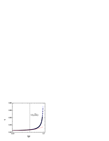
Figure 2: Tunneling time $\tau$ versus the size of the wavepacket in the momentum space, $\Delta p$, for an incident electron with momentum $p_{0}=2.5$ and barrier parameters $V_{0}=5$ and $L=20$. The numerical results are represented by squares, the results based on the presence time formalism by the solid curve and the second order approximation by the dashed curve.

We now extend the previous calculations to the traversal time for photons crossing a set of layers with a frequency gap. In this case, we know that no signal can travel faster than light in vacuum, so this is a good test of the possible constraints in Hartman effect. For electromagnetic waves the expression of $\widehat{T}$ is the same as for electrons but changing the energy by the frequency divided by $\hbar$.

The incident electromagnetic wavepacket moves towards a periodic arrangement of $N-1$ layers. Layers with index of refraction $n_{1}$ and thickness $d_{1}$ alternate with layers of index of refraction $n_{2}$ and width $d_{2}$. For this periodic structure there exits a frequency gap where evanescent modes can be found. The wavenumbers in the layers of the first and second type are $k_{1}=\omega n_{1}/c$ and $k_{2}=\omega n_{2}/c$, respectively. Let us call $a$ the spatial period, so $a=d_{1}+d_{2}$. The periodicity of the system allows us to obtain analytically the transmission amplitude $t_{\rm N}$ using the characteristic determinant method CU96

$$t_{\rm N}=\exp(-ik_{1}d_{1})\times\left\{\cos(N\beta a/2)-i\left(\frac{\sin{(N\beta a/2)}}{\sin(\beta a)}\right)\sqrt{\sin^{2}(\beta a)+\left[{\frac{k_{1}^{2}-k_{2}^{2}}{2k_{1}k_{2}}}\sin(k_{2}d_{2})\right]^{2}}\right\}^{-1},$$ (23)

where $\beta$ plays the role of quasimomentum of the system, and is defined by

$$\cos(\beta a)=\cos(k_{1}d_{1})\cos(k_{2}d_{2})-\left({\frac{k_{1}^{2}+k_{2}^{2}}{2k_{1}k_{2}}}\right)\sin(k_{1}d_{1})\sin(k_{2}d_{2}).$$ (24)

When the modulus of the RHS of Eq. (24) is greater than 1, $\beta$ has to be taken as imaginary. This situation corresponds to a forbidden frequency window. We perform a simulation of the propagation of the wavepacket similar to that for electrons.

In Fig. 3 we represent the traversal time, $\tau$, versus the width of the wavepacket in the wavenumber domain, $\Delta k$, for an incident electromagnetic wavepacket with momentum $k_{0}=3.927$, which corresponds to the centre of the forbidden frequency window of our system. The units are set by the choice $\hbar=c=1$. The periodic arrangement consists of $19$ layers with alternating indices of refraction $2.0$ and $1.0$, and widths $0.6$ and $1.2$, respectively, so the spatial length of the structure is $L=16.8$. This periodic case satisfies the relation $n_{1}d_{1}=n_{2}d_{2}$ and most experimental setups use this periodic arrangement ST93 . The numerical results are represented by squares, while the solid curve corresponds to the results obtained with the presence time formalism. We can see that this curve fits very well the numerical results for all sizes of the incident wavepacket. The dashed curve represents the second order approximation and fits the numerical results relatively well up to values of $1/\sqrt{2}\Delta k$ of the order of the barrier length. The limit of very narrow wavepackets in $\Delta k$ again coincides with the real component of the time obtained with the Green function approach. In the case analyzed, it is much smaller than the crossing time of the structure at the vacuum speed of light, represented by the horizontal line in Fig. 3. The crossing time remains smaller than the vacuum crossing time for sizes of the wavepacket in real space up to half the width of the structure.

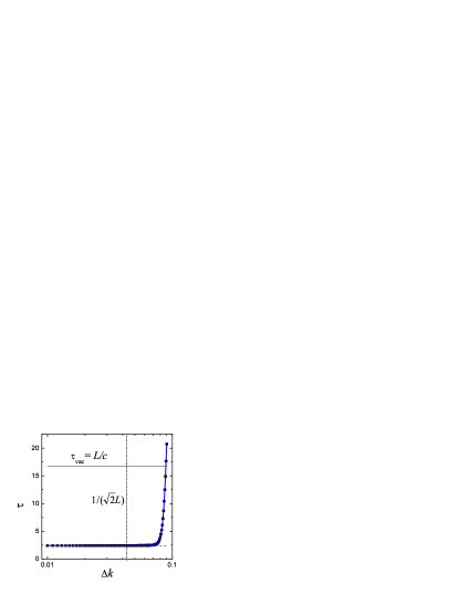
Figure 3: Traversal time $\tau$ versus $\Delta k$ for an electromagnetic wavepacket with $k_{0}=3.927$. The periodic arrangement consists of $19$ layers with alternating indices of refraction $2.0$ and $1.0$, and widths $0.6$ and $1.2$, respectively. The squares represent the results obtained via the wavepacket approach, the solid curve shows the results obtained with the presence time formalism and the dashed curve the second order approximation.

In the circumstances analyzed in the previous paragraph, there is no signal travelling faster than light at vacuum due to the large uncertainty in the time. In Fig. 4 we represent the uncertainty of the tunneling time, $\Delta\tau$, versus the width of incident the wavepacket in the wavenumber domain, $\Delta k$, for the periodic structure of the previous example. The numerical results are shown by squares and the solid curve represents the results obtained via the presence time formalism. We can see that the this curve fits very well the numerical results for all sizes of the incident wavepacket. The dashed curve corresponds to the second order approximation.

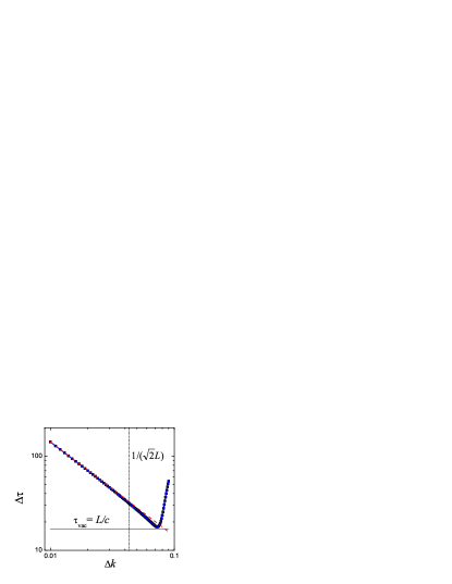
Figure 4: Uncertainty of the tunneling time $\tau$ versus the size of the wavepacket in the wavenumber space, $\Delta k$, for an incident electromagnetic wavepacket with central wavenumber $k_{0}=3.927$. The periodic arrangement is the same as in the previous example. The numerical results are shown by squares and the solid curve represents the results obtained via the presence time formalism. The dashed curve corresponds to the second order approximation.

VI Conclusions

We have used the presence time formalism to calculate the tunneling time and its uncertainty for finite size wave-packets. In the simplest case of a one-dimensional rectangular potential barrier the tunneling time is related to the expectation value of the time operator $\widehat{T}$ at the right side of the barrier, weighted by the transmitted wavepacket in the energy representation, $|\Phi_{\rm III}(L,E)|^{2}$. This expectation value is in turn given by an energy average of the phase time $\tau_{y}(E)$.

For very long wavepackets the presence time formalism produces the same results as previous approaches to the tunneling time problem BT83 ; GO04 . For wavepackets of spatial size of the order of the dimensions of the barrier, the results agree extremely well with numerical simulations of wavepacket evolution. These results are also in quite good agreement with our calculations based on the time of arrival approach by León et al. LE00 . Similar conclusions apply to the traversal time problem of photons through dielectric structures in the frequency gap region.

There is no fundamental problem with Hartman effect, because the uncertainty in the time is larger than the advance in time with respect to its vacuum value, whenever this difference is important RO97 . Our approach is particularly valuable for this type of problems, since it is able to handle finite size effects of wavepackets.

- (1) R. Landauer and Th. Martin, Rev. Mod. Phys. 66, 217 (1994).
- (2) T. E. Hartman, J. Appl. Phys. 33, 3427 (1962).
- (3) I. A. Baz’, Sov. J. Nucl. Phys. 4, 182 (1967).
- (4) I. A. Baz’, Sov. J. Nucl. Phys. 5, 161 (1967).
- (5) M. Büttiker, Phys. Rev. B 27, 6178 (1983).
- (6) V. Gasparian, M. Ortuño, J. Ruiz, and E. Cuevas, Phys. Rev. Lett. 75, 2312 (1995).
- (7) R. Landauer, Nature 365, 692 (1993).
- (8) V. Gasparian and M. Pollak, Phys. Rev. B 47, 2038 (1993).
- (9) V. Gasparian, M. Ortuño, J. Ruiz, E. Cuevas, and M. Pollak, Phys. Rev. B 51, 6743 (1995).
- (10) D. Sokolovski and L. M. Baskin, Phys. Rev. A 36, 4604 (1987).
- (11) D. Sokolovski and J. N. L. Connor, Phys. Rev. A 44, 1500 (1990).
- (12) H. A. Fertig, Phys. Rev. Lett. 65, 2321 (1990).
- (13) A. Auerbach and S. Kivelson, Nucl. Phys. B 257, 799 (1985).
- (14) W. Pauli, in Encyclopedia of Physics., edited by S. Flugge (Springer, Berlin, 1958), Vol. 5.
- (15) J. G. Muga and C. R. Leavens, Phys. Rep. 338, 353 (2000).
- (16) G. R. Allcock, Ann. Phys. (N. Y.) 53, 253 (1969); 53, 286 (1969); 53, 311 (1969).
- (17) R. Werner, J. Math. Phys. 27, 793 (1986).
- (18) J. León, J. Julve, P. Pitanga, and F. J. de Urríes, Phys. Rev. A 61, 062101 (2000).
- (19) A. D. Baute, I. L. Egusquiza and J. G. Muga, Phys. Rev. A 64, 012501 (2001).
- (20) V. S. Olkhovsky, E. Recami and A. J. Gerasimchuk, Il Nuovo Cimento 22, 263 (1974).
- (21) E. Recami, in The Uncertainty Principle and Foundations of Quantum Mechanics, edited by W. C. Price and S. S. Cgissick (Wiley, London, 1977).
- (22) D. H. Kobe and V. C. Aguilera-Navarro, Phys. Rev. A 50, 933 (1994).
- (23) D. H. Kobe, H. Iwamoto, M. Goto and V. C. Aguilera-Navarro, Phys. Rev. A 64, 022104 (2001).
- (24) V. Gasparian, M. Ortuño, and O. del Barco, Encyclopedia of Nanoscience and Nanotechnology 3, (193-215) (2004).
- (25) I. L. Egusquiza and J. G. Muga, Phys. Rev. A 61, 012104 (1999).
- (26) S. Brouard, R. Sala, and J. G. Muga, Phys. Rev. A 49, 4312 (1994).
- (27) E. Cuevas, V. Gasparian, M. Ortuño, and J. Ruiz, Z. Phys. B 100, 595 (1996).
- (28) A. M. Steinberg, P. G. Kwiat, and R. Y. Chiao, Phys. Rev. Lett. 71, 708 (1993).
- (29) J. Ruiz, M. Ortu o, E. Cuevas and V. Gasparian, J. Phys. I France 7, 653 (1997).