Spatial dynamics, thermalization, and gain clamping in a photon condensate

Abstract

We study theoretically the effects of pump-spot size and location on photon condensates. By exploring the inhomogeneous molecular excitation fraction, we make clear the relation between spatial equilibration, gain clamping and thermalization in a photon condensate. This provides a simple understanding of several recent experimental results. We find that as thermalization breaks down, gain clamping is imperfect, leading to “transverse spatial hole burning” and multimode condensation. This opens the possibility of engineering the gain profile to control the condensate structure.

I Introduction

The laser has long served as a prototype for phase transitions in driven dissipative systems Graham and Haken (1970); Haken (1975). While for a single-mode cavity the transition is mean-field-like, in a multimode cavity Staliunas and Sanchez-Morcillo (2003) spatial fluctuations are possible, enabling non-trivial critical behavior. In the last decade, there has been much interest in other examples of phase transitions in driven-dissipative systems. In part, this has been motivated by experiments on polariton condensation Kasprzak et al. (2006); Balili et al. (2007); Carusotto and Ciuti (2013). However, there are also experiments on cold atoms in optical cavities Baumann et al. (2010); Baden et al. (2014), and proposals for experiments in “coupled cavity arrays” Angelakis et al. (2007); Hartmann et al. (2006); Greentree et al. (2006) of superconducting circuits Underwood et al. (2012) or hybrid quantum systems Zou et al. (2014). There are also intriguing connections between the dynamics of these quantum systems, and the study of similar questions on the dynamics of classical “active matter” Marchetti et al. (2013), as studied in photo-excited colloidal systems Palacci et al. (2013). These systems all address common questions of how a flow of energy through the system affects the collective dynamics of the system, and the emergence of spatial structures.

Closely related to both polariton condensates and photon lasers are experiments on Bose-Einstein condensation (BEC) of photons Klaers et al. (2010a) in organic-dye-filled microcavities. Unlike polaritons, these systems have no strong matter-light coupling and so the normal modes are non-interacting photons. However thermalization is possible Klaers et al. (2010b) via the dye molecules. If a photon can be absorbed and emitted many times before it leaves the cavity, the photon gas achieves thermal equilibrium with the dye. Thus, by adjusting the rates of absorption and emission, or cavity decay, one may interpolate between an equilibrium BEC, and a strongly dissipative dye laser Schäfer (1990). We will refer to condensation throughout this paper, but we present phenomena that can be interpreted either as lasing or BEC. Following these experiments many theoretical works Klaers et al. (2012); Sob’yanin (2012); Snoke and Girvin (2013); Kirton and Keeling (2013); Kruchkov (2014); van der Wurff et al. (2014); de Leeuw et al. (2014a); Chiocchetta and Carusotto (2014); Nyman and Szymańska (2014); Sela et al. (2014); Kirton and Keeling (2015); de Leeuw et al. (2014b); Chiocchetta et al. (2015) explored topics including equilibration, phase coherence, and photon statistics of the photon BEC, and later experiments studied photon statistics Schmitt et al. (2014).

Recently, two experiments Marelic and Nyman (2015); Schmitt et al. (2015) studied the spatial profile and dynamics of the photon BEC and their dependence on pump-spot size and location, observing behavior beyond the scope of existing models. Spatial profiles below threshold were also previously studied in Klaers et al. (2010b). These works motivate this paper. Studying spatially varying systems moves away from the domain of simple “mean-field” models of lasing or phase transitions: spatial modes allow for non-mean field critical behavior at phase transitions, and for spatial decay of coherence. This has been explored experimentally for polaritons in one- Wertz et al. (2010) and two-dimensions Roumpos et al. (2012). Considering such critical behavior in extended systems, theoretical work has shown that features beyond the equilibrium classification Hohenberg and Halperin (1977) can arise, such as new critical exponents in three dimensions Sieberer et al. (2013), the destruction of algebraic order in two-dimensional systems Altman et al. (2015), and potential novel universality classes in one dimension Marino and Diehl . Multimode cavity systems — i.e. spatially extended systems — also allow for transverse pattern formation, as has been studied in lasers Staliunas and Sanchez-Morcillo (2003), and for polaritons Manni et al. (2011); Tosi et al. (2012); Nelsen et al. (2013); Gao et al. (2015). Very recently, there has been an experimental realization of a system of cold atoms in a multimode optical cavity Kollár et al. (2015). An important distinction exists between such atomic experiments, where photons couple to density or spin waves of the atoms, with the atom number being conserved, vs exciton-polaritons where photons couple to the exciton itself, creating or destroying excitons. Nonetheless, these systems provide an additional complimentary perspective on the physics of driven-dissipative matter-light systems.

The aim of this paper is to introduce a model capable of describing how the size and shape of the pump profile affects the spatial profile of a photon BEC. In order to describe the spatial profile of a condensate, a widely used approach is to derive order parameter equations, i.e. a partial differential equation determining the time evolution of a field $\Psi(\mathbf{r})$, representing the condensate order parameter. The equations determining the spatial profile of a condensate are distinct for closed (conservative) and open (dissipative) systems. In a closed BEC, this equation is the Gross-Pitaevskii equation Pitaevskii and Stringari (2003) (GPE), which can be written in the form $i\hbar\partial_{t}\psi=\delta E[\Psi]/\delta\Psi^{\ast}$. Such an equation conserves an energy functional $E[\Psi]$, with corresponding phase evolution of the order parameter. In contrast, for a purely dissipative system, the time dependent Ginzburg Landau equation Ginzburg and Landau (1950) (GLE) describes irreversible relaxation, $\partial_{t}\psi=-\Gamma\delta E[\Psi]/\delta\Psi^{\ast}$, so that the final state is a state of minimum energy. A classification of such order parameter equations has been given by Hohenberg and Halperin (1977). Combining both conservative and dissipative terms leads to the complex GPE or GLE Aranson and Kramer (2002), widely used for polariton condensates Wouters and Carusotto (2007); Keeling and Berloff (2008); Wouters et al. (2008). In some cases, such equations can show critical behavior outside the Hohenberg–Halperin classification Sieberer et al. (2013). Similar equations also arise in nonlinear optics Staliunas and Sanchez-Morcillo (2003), where dispersive shifts (i.e. nonlinear dielectric functions, depending on the field amplitude $|\Psi|^{2}$) compete with dissipative terms describing loss and gain; for example, in a class-A laser, the dynamics of the gain medium can be adiabatically eliminated, leading to a complex Ginzburg–Landau equation of motion for the field amplitude Graham and Haken (1970).

In this paper we make use of a different approach, considering density matrix equations of motion, rather than order parameter equations. This is because order parameter equations generally only crudely model relaxation to a thermal state — in particular, the order parameter normally only describes the macroscopically occupied mode(s), and neglects thermal fluctuations. For many examples of pattern formation in nonlinear optics this is entirely appropriate: no thermalization occurs, and this is accurately reproduced by the order parameter equation. However, for photon BEC, thermalization is a key feature of the observed behavior, and so a complete model should be able to explain how this interacts with spatial pattern formation. Extensions of order parameter equations to include energy dependent gain rates have been developed to address this for polaritons Wouters et al. (2010); Wouters (2012). By including also noise terms phenomenologically, these can yield thermal distributions. In this paper we instead follow an approach that proceeds directly from our microscopic model Kirton and Keeling (2013, 2015). We show that for weak coupling one can derive a tractable model combining spatial dynamics with energy relaxation. This model describes how the spatial profile is determined by the competition between energy relaxation and loss, and can explain the recent experiments Marelic and Nyman (2015); Schmitt et al. (2015).

The remainder of this paper is organized as follows. Section II describes our model of the experiments, and derives a master equation for the photon modes and electronic state of the molecules, eliminating the fast dynamics of molecular vibrations. From this model, we derive coupled equations for the population of excited molecules, and the populations and coherence of photon modes. Using these equations, section III discusses the steady state properties of the photon cloud. In Sec. III.1 we first show how, far below threshold, the occupation of photon modes depends both on their energy (controlling the rate of emission and absorption for that mode), and also the overlap between the photon mode and the profile of the pump. This behavior occurs at weak pumping because there the excitation profile of molecules follows that of the pump. The same approach allows us to understand how the pump profile affects the threshold power required for condensation, discussed in Sec. III.2. Once above threshold, the profile of excited molecules is significantly modified by the condensed photons, via a kind of transverse spatial hole burning. We discuss the consequences of this in Sec. III.3. In Section IV we then turn to study the early-time transient dynamics of a condensate following an off-center pump. We show how the spatial oscillations evolve due to reabsorption of cavity light, leading ultimately to thermalization. Finally, section V provides some conclusions and outlook from our work.

II Model

The photon BEC system consists of dye molecules coupled to photon modes in an optical cavity (see Fig. 1(a). Each molecule has a complex optical spectra, due to the ro-vibrational dressing of the electronic spectrum. Despite this, one can nonetheless consider only two electronic states, the highest occupied molecular orbital (HOMO) and lowest unoccupied molecular orbital (LUMO). Each of these levels is however dressed by ladder(s) of rotational and vibrational excitations of the molecules. As discussed in our previous work Kirton and Keeling (2013, 2015), one may adiabatically eliminate the vibrational states, leading to absorption and emission rates $\Gamma(\pm\delta)$ for photon modes detuned by $\delta=\omega-\omega_{\text{ZPL}}$ from the Zero Phonon Line (ZPL) of the molecule. This results in a model in which the electronic state (HOMO or LUMO) of each molecule is explicitly represented, while the effects of the ro-vibrational excitations appear implicitly in the structure of the rates $\Gamma(\pm\delta)$ discussed further below.

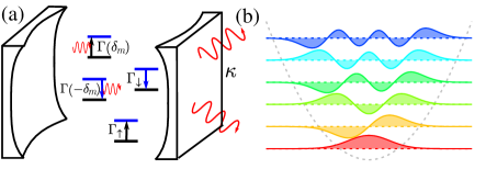
Figure 1: (Color online) (a) Cartoon of model system: molecules are represented by two electronic states (HOMO and LUMO levels), dressed by ro-vibrational excitations. (b) Gauss-Hermite eigenfunctions of an harmonic oscillator.

To incorporate inhomogeneous pumping we must consider the overlap $\psi_{m}(\mathbf{r}_{i})$ between the transverse mode function of photon mode $m$ and a molecule at $\mathbf{r}_{i}$. We do not include here effects of the longitudinal mode profile, as we consider cases where only a single longitudinal mode is relevant (i.e. close enough to resonance with the gain medium). In these cases, except for very high order modes, the longitudinal mode profile does not vary significantly between the modes, and so any effects of overlap between the longitudinal mode profile and the excited molecules can be absorbed into a constant factor in the definition of emission and absorption rates. For the transverse modes, curvature of the cavity mirrors leads to an in-plane harmonic trap, so that $\psi_{m}(\mathbf{r})$ are Gauss-Hermite functions (see Fig. 1(b)) in two dimensions and the corresponding frequencies are harmonically spaced, $\omega_{m}=\omega_{c}+(m_{x}+m_{y})\epsilon$, where $m$ combines both $m_{x}$ and $m_{y}$ indices. The “cavity cutoff” $\omega_{c}$ is set by the cavity length. We write the master equation describing the system as two terms, $\partial_{t}\hat{\rho}=\mathcal{M}_{0}[\hat{\rho}]+\mathcal{M}_{\text{int}}[\hat{\rho}]$. The bare part is:

$$\mathcal{M}_{0}[\hat{\rho}]=-i\sum_{m}\left[\omega_{m}\hat{a}^{\dagger}_{m}\hat{a}_{m},\hat{\rho}\right]+\sum_{m}\frac{\kappa}{2}\mathcal{L}[\hat{a}_{m},\hat{\rho}]\\ +\sum_{i}\frac{\Gamma_{\uparrow}(\mathbf{r}_{i})}{2}\mathcal{L}[\hat{\sigma}^{+}_{i},\hat{\rho}]+\sum_{i}\frac{\Gamma_{\downarrow}}{2}\mathcal{L}[\hat{\sigma}^{-}_{i},\hat{\rho}],$$ (1)

where $\mathcal{L}[\hat{X},\hat{\rho}]=2\hat{X}^{\dagger}\hat{\rho}\hat{X}-[\hat{X}^{\dagger}\hat{X},\hat{\rho}]_{+}$. The operator $\hat{a}^{\dagger}_{m}$ creates a photon in mode $m$, and we assume all modes have decay rate $\kappa$. The electronic state of molecule $i$ is represented by Pauli operators $\hat{\sigma}_{i}^{x,y,z}$. In addition to coupling to the cavity (see below), each molecule has a pumping rate $\Gamma_{\uparrow}(\mathbf{r}_{i})$, and a non-cavity decay rate $\Gamma_{\downarrow}$ incorporating fluorescence into all modes other than the confined cavity modes. Other than the inhomogeneous pump, $\mathcal{M}_{0}[\hat{\rho}]$ matches Refs. Kirton and Keeling (2013, 2015).

The term $\mathcal{M}_{\text{int}}[\hat{\rho}]$, describing molecule-photon interaction, can be treated at various levels of approximation, according to whether we include coherence between different photons modes. Including such inter-mode coherence is numerically expensive, and is only necessary when significant coherence exists. The numerical cost arises because, if we truncate the equations to consider $N_{m}$ photon modes, the full coherence matrix scales as $N_{m}^{2}$. As discussed later, in order to keep all significantly populated modes (when $k_{B}T\gg\hbar\epsilon$), we need relatively large values of $N_{m}$. Thus, with the full equations, it is only feasible to simulate a few hundred picoseconds of time evolution, far shorter than the timescale required to reach the steady state. In what follows, we therefore first present the full equations of motion, used to study transient dynamics, and then introduce the “diagonal approximation”, providing a more efficient approach when inter-mode coherence can be neglected.

II.1 Fully coherent model

We denote the most complete form of the molecule-photon interaction $\mathcal{M}_{\text{int}}[\hat{\rho}]=\mathcal{M}_{\text{int}}^{\text{full}}[\hat{\rho}]$, which takes the form:

$$\mathcal{M}^{\text{full}}_{\text{int}}[\hat{\rho}]\equiv\!\!\sum_{m,m^{\prime},i}\!\!\psi^{\ast}_{m}(\mathbf{r}_{i})\psi_{m^{\prime}}(\mathbf{r}_{i})\bigl{\{}K(\delta_{m^{\prime}})[\hat{a}_{m^{\prime}}\hat{\sigma}_{i}^{+}\hat{\rho},\hat{a}_{m}^{\dagger}\hat{\sigma}^{-}_{i}]\\ +K(-\delta_{m})[\hat{a}^{\dagger}_{m}\hat{\sigma}_{i}^{-}\hat{\rho},\hat{a}_{m^{\prime}}\hat{\sigma}_{i}^{+}]\bigr{\}}+\text{H.c.}.$$ (2)

The complex function $K(\pm\delta_{m})$, discussed next, encodes the molecular absorption (emission) rate vs. the detuning $\delta_{m}=\omega_{m}-\omega_{\text{ZPL}}$ between mode $m$ and the molecular Zero Phonon Line (see dashed line in Fig. 2).

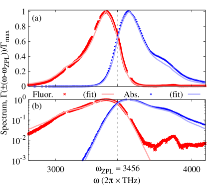
Figure 2: (Color online) (a) Absorption and fluorescence spectrum of Rhodamine 6G on a (a) linear or (b) logarithmic scale. Points are experimental data Nyman and Marelic (for dye in Ethylene Glycol), lines show the fits $\Gamma(\pm\delta)$ satisfying $\Gamma(\delta)=\Gamma(-\delta)e^{\beta\delta}$ at room temperature. Here and throughout, we plot angular frequency, $\omega=2\pi f$. To indicate this we write the units as $2\pi$THz.

For simple molecules, $K(\delta)$ can be calculated explicitly Kirton and Keeling (2015). Alternatively, one may use experimentally measured spectra $\Gamma(\delta)$, and find $K(\delta)$ by analytic continuation — causality requires that $K(\delta)$ is analytic in the lower half plane. As noted previously Klaers et al. (2010b, a); Kirton and Keeling (2013), thermalization of photons requires that $\Gamma(\delta)$ obeys the Kennard-Stepanov (KS) relation Kennard (1918, 1926); Stepanov (1957), $\Gamma(\delta)=\Gamma(-\delta)e^{\beta\delta}$. We therefore use a function $\Gamma(\delta)$, shown in Fig. 2, that fits the experimental spectra, while satisfying the KS relation. The procedure used is described in appendix A. This determines $\Gamma(\delta)$ up to a prefactor. We denote $\Gamma_{\text{max}}=\text{max}[\Gamma(\delta)]$, and discuss below how to estimate $\Gamma_{\text{max}}$ from experimental results. The function $K(\delta)$ is then found by standard analytic continuation of $\Gamma(\delta)$ to the lower half plane.

Note that while equation (2) includes coherence between photon modes, it neglects coherence between molecules. This is because dye and solvent molecules collide frequently causing rapid dephasing. Inter-mode coherence will be required to understand the dynamics, as studied experimentally in Ref. Schmitt et al. (2015). It is important also to note that by including inter-mode coherences, equation (2) does not make the “secular approximation”, which discards those bath-induced terms which are time dependent in the interaction picture. The secular approximation is often introduced as a necessary condition for having a completely positive master equation Dümcke and Spohn (1979). However several recent papers suggest the secular approximation can lead to incorrect predictions Jeske et al. (2015); Joshi et al. (2014); Eastham et al. . As discussed later, the current model falls into this class: the experimentally observed oscillations of the photon density can only occur if the molecular emission produces inter-mode coherence — an incoherent state would show no beating. Beyond the secular approximation, there may be instabilities, particularly at large $\Gamma_{\text{max}}$. However, for large $\Gamma_{\text{max}}$ the Markov approximation fails Eastham et al. . For the parameters we consider, our equations are stable.

Rather than explicitly simulating the density matrix $\hat{\rho}$, we use the master equation above to write coupled equations of motion for the (Hermitian) photon correlation matrix $[\mathbf{n}]_{m,m^{\prime}}=\langle\hat{a}^{\dagger}_{m}\hat{a}_{m^{\prime}}\rangle$, and the coarse-grained excitation density, $f(\mathbf{r})=\sum_{i}\delta(\mathbf{r}-\mathbf{r}_{i})\langle\hat{\sigma}^{+}_{i}\hat{\sigma}^{-}_{i}\rangle$. Within the semiclassical approximation Kirton and Keeling (2015) $[\mathbf{n}]_{m,m^{\prime}}$ and $f(\mathbf{r})$ obey a closed set of equations. The semiclassical approximation means that we neglect correlations between the state of the photons and the dye molecules, so that expectations of products of operators can be replaced by products of expectations. These semiclassical equations can be written in a particularly compact form by defining a number of other quantities. We define the matrices $[\mathbf{K}_{\pm}]_{m,m^{\prime}}\equiv\delta_{m,m^{\prime}}K(\pm\delta_{m})$, the mode function matrix $[\mathbf{\Psi}(\mathbf{r})]_{m,m^{\prime}}\equiv\psi_{m}(\mathbf{r})\psi_{m^{\prime}}(\mathbf{r})$, the overlap matrix $\mathbf{f}\equiv\int d^{d}\mathbf{r}f(\mathbf{r})\mathbf{\Psi}(\mathbf{r})$ and $[\mathbf{h}]_{m,m^{\prime}}\equiv\delta_{m,m^{\prime}}(i\omega_{m}-\kappa)$. We thus write the equations:

$$\partial_{t}\mathbf{n}=\mathbf{h}\mathbf{n}+\mathbf{f}\rho_{0}\mathbf{K}_{-}(\mathbf{n}+\mathbbm{1})+(\mathbf{f}-\mathbbm{1})\rho_{0}\mathbf{K}_{+}^{\dagger}\mathbf{n}+\text{H.c.},$$ (3)

$$\partial_{t}f(\mathbf{r})=-\Gamma_{\downarrow}^{\text{tot}}(\mathbf{n},\mathbf{r})f(\mathbf{r})+\Gamma_{\uparrow}^{\text{tot}}(\mathbf{n},\mathbf{r})(1-f(\mathbf{r})),$$ (4)

where $\rho_{0}$ is the density of molecules. Note that in the first equation, while $\mathbf{n},\mathbf{f}$ are Hermitian, the matrices $\mathbf{h},\mathbf{K}_{\pm}$ are not. In the equation for the excitation density $f(\mathbf{r})$, the total absorption and emission rates are:

$$\Gamma_{\uparrow}^{\text{tot}}(\mathbf{n},\mathbf{r}) =\Gamma_{\uparrow}(\mathbf{r})+2\Re\left(\text{Tr}\left[\mathbf{\Psi}(\mathbf{r})\mathbf{n}\mathbf{K}_{+}\right]\right)$$ (5)

$$\Gamma_{\downarrow}^{\text{tot}}(\mathbf{n},\mathbf{r}) =\Gamma_{\downarrow}+2\Re\left(\text{Tr}\left[\mathbf{\Psi}(\mathbf{r})\mathbf{K}_{-}(\mathbf{n}+\mathbf{1})\right]\right),$$ (6)

incorporating also stimulated emission to and absorption from the cavity modes. To simulate these equations numerically, we discretize $f(\mathbf{r})$ on a grid of $N_{x}$ spatial points, and then use an adaptive time-step Runge-Kutta approach to evolve the coupled equations.

From these equations, we are typically interested in deriving quantities such as the photon spectrum, and the photon density profile $I(\mathbf{r})$ which is our focus in this paper. These quantities can be directly extracted from the photon correlation matrix. The spectrum is given by the diagonal elements $[\mathbf{n}]_{m,m}$ and the photon density by

$$I(\mathbf{r})=\sum_{m,m^{\prime}}\psi^{\ast}_{m}(\mathbf{r})\psi_{m^{\prime}}(\mathbf{r})[\mathbf{n}]_{m,m^{\prime}}.$$

Simulating the full state of the system would thus require solving $N_{m}^{2}+N_{x}$ coupled differential equations. One can reduce this requirement by noting that elements of $[\mathbf{n}]_{m,m^{\prime}}$ that are far from the diagonal are however very small. As discussed earlier, the value of $N_{m}$ required is however relatively large; and even with reduction to terms with small $|m-m^{\prime}|$, we find it is only feasible to simulate short-time transient behavior, and only in one spatial dimension. The results presented later involved $150$ps of simulated time requiring four hours of computer time, while the timescale to reach steady state is of the order of microseconds.

II.2 Diagonal approximation

As noted at the end of the last section, the full equations are too computationally costly to allow numerical exploration of how the steady state profile depends on control parameters. To overcome this limitation, we introduce here the “diagonal approximation”, which is accurate as long as coherence between photon modes is small, and allows numerical exploration of the steady state. This corresponds to using the molecule-photon interaction $\mathcal{M}_{\text{int}}[\hat{\rho}]=\mathcal{M}_{\text{int}}^{\text{diag}}[\hat{\rho}]$ with

$$\mathcal{M}_{\text{int}}^{\text{diag}}[\hat{\rho}]\equiv-i[H_{\Lambda},\hat{\rho}]+\frac{1}{2}\sum_{m,i}{|\psi_{m}(\mathbf{r}_{i})|^{2}}\times\\ \biggl{(}\Gamma(\delta_{m})\mathcal{L}[\hat{a}_{m}\hat{\sigma}_{i}^{+},\rho]+\Gamma(-\delta_{m})\mathcal{L}[\hat{a}^{\dagger}_{m}\hat{\sigma}_{i}^{-},\rho]\biggr{)}$$ (7)

where $\Gamma(\pm\delta)\equiv 2\Re[K(\pm\delta)]$ are the absorption(emission) rates, and $H_{\Lambda}$ is a Lamb shift from the imaginary part of $K(\pm\delta)$. This Lamb shift will however be irrelevant for the equations of motion as discussed next.

In this approximation, we may write closed equations for the populations of the photon modes, neglecting coherences, and thus have only $N_{m}+N_{x}$ equations. Denoting the diagonal elements of the correlation matrix as $n_{m}=[\mathbf{n}]_{m,m}$, and the diagonal overlap elements as $f_{m}\equiv[\mathbf{f}]_{m,m}=\int d^{d}{\mathbf{r}}f(\mathbf{r})|\psi_{m}(\mathbf{r})|^{2}$, these coupled equations take the form:

$$\partial_{t}n_{m} =\rho_{0}\Gamma(-\delta_{m})f_{m}(n_{m}+1)$$

$$\qquad\qquad-\left[\kappa+\rho_{0}\Gamma(\delta_{m})(1-f_{m})\right]n_{m},$$ (8)

$$\partial_{t}f(\mathbf{r}) =-\Gamma_{\downarrow}^{\text{tot}}(\{n_{m}\},\mathbf{r})f(\mathbf{r})+\Gamma_{\uparrow}^{\text{tot}}(\{n_{m}\},\mathbf{r})(1-f(\mathbf{r})).$$ (9)

Note here that the second equation, Eq. (9), is identical to that seen previously, however the total molecular excitation and decay rates are now written in terms of the diagonal populations are:

$$\Gamma_{\downarrow}^{\text{tot}}(\{n_{m}\},\mathbf{r}) =\Gamma_{\downarrow}+\sum_{m}|\psi_{m}(\mathbf{r})|^{2}\Gamma(-\delta_{m})(n_{m}+1),$$ (10)

$$\Gamma_{\uparrow}^{\text{tot}}(\{n_{m}\},\mathbf{r}) =\Gamma_{\uparrow}(\mathbf{r})+\sum_{m}|\psi_{m}(\mathbf{r})|^{2}\Gamma(\delta_{m})n_{m}.$$ (11)

In all the equations above we have kept the spatial dimension general, writing generic wavefunctions $\psi_{m}(\mathbf{r})$. The experiments are in two dimensions, in which case the mode functions should take the form:

$$\psi_{m}(\mathbf{r})=\frac{{H}_{m_{x}}\left(\frac{x}{\ell_{\text{HO}}}\right){H}_{m_{y}}\left(\frac{y}{\ell_{\text{HO}}}\right)e^{-r^{2}/2\ell_{\text{HO}}^{2}}}{\ell_{\text{HO}}\sqrt{\pi 2^{m_{x}+m_{y}}m_{x}!m_{y}!}},$$

where we take $m=(m_{x},m_{y})$ as a combined index and $H_{m}(x)$ is the $m$th Hermite polynomial. In certain cases, it is possible to efficiently find the steady states in two dimensions, and where this is possible, we follow this approach. However, when directly solving the equations of motion, it is intractable to keep all two dimensional modes with energies $\hbar\omega<k_{B}T$, and so in some cases below we instead restrict to one dimension, for which:

$$\psi_{m}(x)=\frac{1}{\sqrt{\ell_{\text{HO}}\sqrt{\pi}2^{m}m!}}{H}_{m}\left(\frac{x}{\ell_{\text{HO}}}\right)e^{-x^{2}/2\ell_{\text{HO}}^{2}}.$$

In the following we will present analytic results for general dimension $d$, and specify $d=1$ or $d=2$ for the numerical results.

III Steady state

In the following we explore the consequences of a finite size Gaussian pump spot,

$$\Gamma_{\uparrow}(\mathbf{r})=\frac{\Gamma_{\uparrow}^{\text{int}}}{(2\pi\sigma_{P}^{2})^{d/2}}\exp\left[-\frac{(\mathbf{r}-\mathbf{r}_{P})^{2}}{2\sigma_{P}^{2}}\right],$$

where $\Gamma_{\uparrow}^{\text{int}}$ is the integrated intensity, $\sigma_{P}$ the spot size, $\mathbf{r}_{P}$ the offset, and $d$ the dimension. Note that $\Gamma_{\uparrow}^{\text{int}}$ has dimensions of $[T]^{-1}[L]^{d}$. Similarly, since $\Gamma(\pm\delta)$ are multiplied by $\rho_{0}$ or $|\psi_{m}(\mathbf{r})|^{2}$, this means $\Gamma_{\text{max}}$ also has dimensions $[T]^{-1}[L]^{d}$. We measure all lengths in units of the oscillator length $\ell_{\text{HO}}$ of the harmonic trap potential, and measure all ($d$-dimensional) densities in units of $\ell_{\text{HO}}^{-d}$. For comparison to Ref. Marelic and Nyman (2015), in the first part of this paper we set $\mathbf{r}_{P}=0$.

III.1 Far below threshold

Far below threshold, when $\Gamma_{\uparrow}(\mathbf{r}=0)\ll\Gamma_{\downarrow}$, both $n_{m}$ and $f(\mathbf{r})$ are small, so the steady state of Eq. (II.2,4) is

$$f(\mathbf{r})\simeq\frac{\Gamma_{\uparrow}(\mathbf{r})}{\Gamma_{\downarrow}^{\text{tot}}(\{n_{m}=0\},\mathbf{r})},\quad n_{m}\simeq f_{m}\frac{\Gamma(-\delta_{m})}{\Gamma(\delta_{m})+\kappa/\rho_{0}}.$$ (12)

Note that in the denominator of the expression for $f(\mathbf{r})$ we have not written $\Gamma_{\downarrow}$, but rather $\Gamma_{\downarrow}^{\text{tot}}(\{n_{m}=0\},\mathbf{r})$, which includes also the spontaneous emission into empty cavity modes. However, for relevant parameters (see below), the cavity mode contribution to $\Gamma_{\downarrow}^{\text{tot}}(\{n_{m}=0\},\mathbf{r})$ is small, so $f(\mathbf{r})\simeq\Gamma_{\uparrow}(\mathbf{r})/\Gamma_{\downarrow}$, and the overlaps $f_{m}$ depend on the pump shape. In this limit the shape of $I(\mathbf{r})$ depends only on the shape of the pump, the normalized spectrum $\Gamma(\pm\delta)/\Gamma_{\text{max}}$, and the dimensionless parameter $\eta\equiv\kappa/\rho_{0}\Gamma_{\text{max}}$. If $\eta\ll 1$ and the KS relation is obeyed then: $n_{m}=f_{m}e^{-\beta\delta_{m}}$. If one also has $\sigma_{P}\gg\ell_{\text{HO}}$, then $f_{m}$ is independent of $m$, and so there is a thermal photon distribution leading to a thermal photon cloud profile:

$$I(\mathbf{r})\propto\sum_{m}e^{-\beta\delta_{m}}|\psi_{m}(\mathbf{r})|^{2}\propto\exp\left(-\frac{r^{2}}{2\sigma_{T}^{2}}\right),$$

with $\sigma_{T}=l_{\text{HO}}/\sqrt{2\tanh(\beta\epsilon/2)}$, which recovers the classical thermal cloud size if $k_{B}T\gg\epsilon$, see Fig. 3(a).

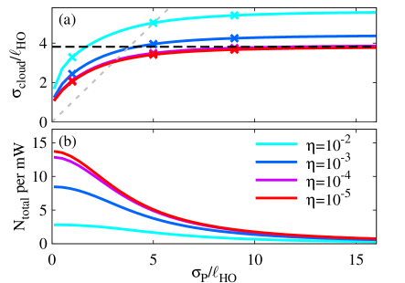
Figure 3: (Color online) (a) Photon cloud size and (b) photon number (per unit power) vs pump-spot size, for various $\eta\equiv\kappa/\rho_{0}\Gamma_{\text{max}}$. Note that in panel (a), the lines for the two smallest values of $\eta$ lie on top of each other. Plotted for $d=2$, far below threshold using the closed-form solution in Eq. (12) with $\omega_{c}=3200$THz. Dashed lines in (a) show thermal size $\sigma_{T}$ (see text) and pump size $\sigma_{P}$. The points marked by the symbols correspond to the points for which cross-sections are shown in Fig. 4.

Thermalization fails for small $\sigma_{P}$ or large $\eta$. This can be seen by looking at the actual cloud profiles, as shown in Fig. 4. At small $\sigma_{P}$ this failure is due to the mode dependence of $f_{m}$: A small pump spot populates only the low order photon modes, leading to an unnaturally small (i.e. cold) photon cloud, even when $\eta\ll 1$ (see Fig. 4(a)). Note that for this non-thermal distribution to occur in this limit, the presence of the non-cavity decay rate $\Gamma_{\downarrow}$ is crucial: if both sources of loss $\Gamma_{\downarrow}$ and $\kappa$ are small, repeated absorption and re-emission of photons will occur, producing a thermal distribution. For large $\eta$ thermalization fails because $n_{m}\simeq f_{m}\Gamma(-\delta_{m})/\kappa\rho_{0}$, and so no Boltzmann factor arises. In Fig. 3(a) this gives a photon cloud which is larger than $\sigma_{T}$ (see outermost (cyan) line in all panels of Fig. 4).

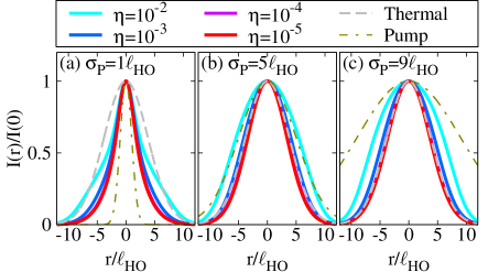
Figure 4: (Color online) Photon cloud profile far below threshold for various $\eta\equiv\kappa/\rho_{0}\Gamma_{\text{max}}$. Note that in all panels, the lines for two smallest values of $\eta$ are indistinguishable. The gray dashed line indicates the equilibrium profile, and the dash-dotted line indicates the profile of the pump spot. Plotted for $\sigma_{P}/\ell_{\text{HO}}=1,5,9$ respectively (a-c) and other parameters as in Fig. 3.

Figure 3(b) shows the total photon number (per unit of incident power) vs pump spot size. For large spots, the number falls off as $(\sigma_{P})^{-d}$. This is because for all modes $m$ with extent much smaller than $\sigma_{P}$, one may approximate

$$f_{m}\simeq\frac{\Gamma_{\uparrow}(\mathbf{r}=0)}{\Gamma_{\downarrow}}=\frac{\Gamma_{\uparrow}^{\text{int}}}{\Gamma_{\downarrow}(\sqrt{2\pi}\sigma_{P})^{d}},$$ (13)

thus giving $N_{\text{total}}/\Gamma_{\uparrow}^{\text{int}}\equiv\sum_{m}f_{m}e^{-\beta\delta_{m}}/\Gamma_{\uparrow}^{\text{int}}\propto\sigma_{P}^{-d}$. In contrast, for small spots, the number saturates; here $\sigma_{P}$ is much smaller than the extent of the relevant modes and so $f_{m}\simeq|\psi_{m}(\mathbf{r}=0)|^{2}\Gamma_{\uparrow}^{\text{int}}/\Gamma_{\downarrow}$, independent of $\sigma_{P}$. This expression clearly means that the occupation of all odd modes (which have a node at $\mathbf{r}=0$) will vanish. Even modes however have a value for $\psi_{m}(\mathbf{r}=0)$, and so $N_{\text{total}}$ clearly saturates at a finite value. Once $\sigma_{P}\ll\ell_{\text{HO}}$, this overlap with even modes becomes independent of $\sigma_{P}$, leading to the saturation observed in Fig. 3. In experiment Marelic and Nyman (2015), the total photon number initially increases with spot size, an effect not seen here. Such a discrepancy could perhaps arise if the coupling of small pump spots into the cavity is less efficient due to some aspect of the pumping optics: given the above arguments about overlaps for small pumping spots, it is hard to explain such a low efficiency when considering purely light trapped inside the cavity.

The behavior in Fig. 3(a) for $\eta\simeq 10^{-3}$ is very similar to the experimental results of Ref. Marelic and Nyman (2015). Using other known parameters of this experiment, $\rho_{0}\simeq 10^{8}\ell_{\text{HO}}^{-2}$, and $\kappa=500$MHz, this gives $\Gamma_{\text{max}}=5$kHz$\ell_{\text{HO}}^{2}$. We use these parameter values below unless otherwise stated. In order to verify the assumption made earlier that we may replace $\Gamma_{\downarrow}^{\text{tot}}(\{n_{m}=0\},\mathbf{r})\simeq\Gamma_{\downarrow}$, we use these values to estimate the effect of loss into empty cavity modes. Comparing the rate of emission into the lowest cavity mode, $\Gamma(-\delta_{m})|\psi_{0}(\mathbf{r}=0)|^{2}<\Gamma_{\text{max}}/(\sqrt{\pi}\ell_{\text{HO}}^{2})\simeq 2.8$kHz, to the observed background decay rate $\Gamma_{\downarrow}\simeq 250$MHz, this implies that even if the first $1000$ cavity modes contributed to the emission equally, the cavity-mediated contribution would be far smaller than the background. The contribution of high order cavity modes however falls off due both to the overlap $\psi_{m}(\mathbf{r})$, and the eventual decay of $\Gamma(-\delta_{m})$ at large $m$. Thus, the assumptions made at the start of this section are indeed justified.

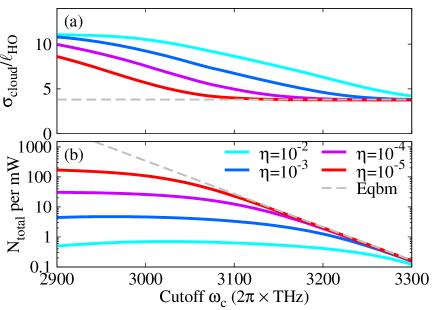
Figure 5: (Color online) (a) Photon cloud size and (b) photon number (per unit power) vs cavity cutoff $\omega_{c}$ for various $\eta\equiv\kappa/\rho_{0}\Gamma_{\text{max}}$. For comparison to later figures, this is plotted for d=1. Spot size $\sigma_{P}=16\ell_{\text{HO}}$; all other parameters as in Fig. 3.

So far in this section we have explored dependence on the properties of the pump spot. Another relatively easy parameter to tune is the cavity cutoff frequency $\omega_{c}$. Indeed, as discussed extensively by Schmitt et al. (2015), tuning this parameter can be used to control the degree of thermalization. A large value of $\omega_{c}$ will enhance reabsorption of cavity and thus lead to thermalization, while a smaller value reduces reabsorption and prevents equilibration. Later in this paper we discuss this behavior at and above threshold. Figure 5 shows the effect of cutoff frequency on properties far below threshold. One can clearly see in Fig. 5(a) that at large $\omega_{c}$, the photon cloud size approaches the equilibrium cloud size. Similarly, considering the total number of photons, one sees that at large $\omega_{c}$ the behavior asymptotically approaches the equilibrium result $N=\sum_{m}f_{m}e^{-\beta\delta_{m}}$ indicated by the gray dashed line (where $f_{m}$ is given by Eq. (13) as we consider a large cloud size, $\sigma_{P}\gg\ell_{\text{HO}}$). At smaller $\omega_{c}$, the photon number decreases as $N\simeq\sum_{m}f_{m}\Gamma(-\delta_{m})\rho_{0}/\kappa$, hence the strong dependence seen upon the value of $\eta=\kappa/\rho_{0}\Gamma_{\text{max}}$.

III.2 Threshold pump power

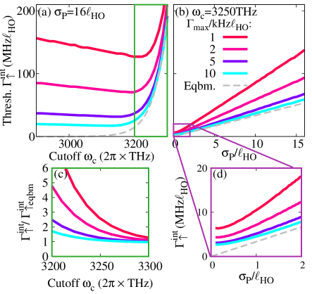
Figure 6: (Color online) Threshold (integrated) pump power, calculated in $d=1$ for various values of $\Gamma_{\text{max}}$. (a) vs cavity cutoff, $\omega_{c}$, (b) vs pump spot size. Simulations performed in one spatial dimension with $N_{m}=200$ photon modes, and $N_{x}=300$ spatial grid points. The dashed line shows the equilibrium result $\Gamma_{\uparrow}^{\text{int}}\equiv\sqrt{2\pi}\sigma_{P}\Gamma_{\uparrow}(r=0)=\sqrt{2\pi}\sigma_{P}\Gamma_{\downarrow}e^{\beta\delta_{c}}$. At large spot sizes, the threshold power increases as $(\sigma_{P})^{d}$ and so is linear for this 1D simulation. Panel (c) shows the ratio of threshold power vs equilibrium threshold power for the region highlighted in panel (a), illustrating the asymptotic approach to equilibrium. Panel (d) shows an enlarged region from panel (b) as indicated.

We next turn to the behavior at threshold, and explore how this depends on the pump size. As with any finite size system, the threshold is not perfectly sharp; for definiteness we use the same threshold condition defined in Refs. Kirton and Keeling (2013, 2015). Figure 6 shows the threshold value of $\Gamma_{\uparrow}^{\text{int}}$ vs cavity cutoff, $\omega_{c}$, and vs pump spot size, $\sigma_{P}$. These calculations, time-evolving Eqs. (II.2–11) numerically, are computationally expensive in $d=2$ so we consider $d=1$ from hereon. In equilibrium the threshold condition is $\Gamma_{\uparrow}(\mathbf{r}=0)=\Gamma_{\downarrow}e^{\beta\delta_{c}}$, where $\delta_{c}=\omega_{c}-\omega_{\text{ZPL}}$ (see Kirton and Keeling (2013)). This condition has a simple meaning: it identifies when the effective chemical potential of the molecules, $\mu_{\text{eff}}(\mathbf{r})=\omega_{\text{ZPL}}+k_{B}T\ln[\Gamma_{\uparrow}(\mathbf{r})/\Gamma_{\downarrow}]$ reaches the lowest photon mode Kirton and Keeling (2015), $\omega_{c}$.

As has been discussed previously Marthaler et al. (2011); Kirton and Keeling (2013, 2015), it is notable that the lasing transition, normally associated with inversion, can be described here as corresponding to a thermal distribution with a positive temperature and chemical potential $\mu_{\text{eff}}<\omega_{\text{ZPL}}$. The fundamental reason why electronic inversion is not required here is the different rates of absorption and emission, $\Gamma(\pm\delta)$. Net inversion of the electronic state is normally required for lasing because absorption and emission coefficients match, so net gain requires an inverted population. Here, for modes with $\delta=\omega-\omega_{\text{ZPL}}<0$, we have $\Gamma(-\delta)>\Gamma(\delta)$, and so for these modes, emission exceeds absorption even without electronic inversion. If one considers the microscopic ro-vibronic levels of the molecule, there is inversion between the lowest ro-vibrational level of the electronic excited state, and the higher ro-vibrational levels of the electronic excited states, and it is these transitions that have net gain Schäfer (1990). However, in our model, the fast dynamics of the ro-vibrational levels have been adiabatically eliminated.

The thermal equilibrium prediction of threshold at $\mu_{\text{eff}}(\mathbf{r}=0)=\omega_{c}$ is shown as the dashed line in Fig. 6. The actual threshold in Fig. 6(a) is however non-monotonic. At large $\omega_{c}$ the system is thermal, and so threshold increases exponentially with $\omega_{c}$. Figure 6(c) illustrates the asymptotic approach to the equilibrium behaviour by plotting the ratio $\Gamma_{\uparrow}^{\text{int}}/(\sqrt{2\pi}\sigma_{P}\Gamma_{\downarrow}e^{\beta\delta_{c}})$, which approaches $1$ at large $\omega_{c}$. At small $\omega_{c}$ the absorption and emission rates are too small to compete with cavity loss, and so the threshold pump increases. Such non-monotonic dependence has been seen experimentally Marelic and Nyman (2015). The minimum of threshold becomes more pronounced as one increases the cavity loss rate $\kappa$ or decreases the peak emission rate $\Gamma_{\text{max}}$.

In Figure 6(b), we see that in $d=1$, $\Gamma_{\uparrow}^{\text{int}}\propto\sigma_{P}$ at threshold, except for small spot sizes where it saturates (see the enlarged region in Fig. 6(d)). From the asymptotic form of the equations it is straightforward to see that in $d$ dimensions this result becomes $\Gamma_{\uparrow}^{\text{int}}\propto(\sigma_{P})^{d}$. Such a dependence on spot size occurs because threshold is reached first at the trap center, where $\mu_{\text{eff}}(\mathbf{r})$ is greatest. As such, it is the peak pump power $\propto\Gamma_{\uparrow}^{\text{int}}\sigma_{P}^{-d}$ that enters the threshold condition. It is however important to note that the simple power law arises only for large enough spot sizes, whereas for spot sizes comparable to the harmonic oscillator length, saturation of the critical integrated power occurs. In the (two dimensional) experiment of Ref. Marelic and Nyman (2015) a phenomenological power law with exponent $\sim 1.5$ was extracted from a least squares plot to data on a log-log scale over one decade of spot size.

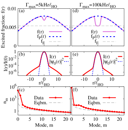
Figure 7: (Color online) Clamping of the gain profile for sufficiently large $\Gamma_{\text{max}}$ (in $d=1$). Panels (a,b,c) show $\Gamma_{\text{max}}=5$kHz$\ell_{\text{HO}}$, panels (d,e,f) $\Gamma_{\text{max}}=100$kHz$\ell_{\text{HO}}$. Top panels show the gain profile $f(\mathbf{r})$ (solid), the value set by the pump, $f_{P}(\mathbf{r})=\Gamma_{\uparrow}(\mathbf{r})/(\Gamma_{\downarrow}+\Gamma_{\uparrow}(\mathbf{r}))$ (short dashed), and the clamped value $f_{E}=[e^{-\beta\delta_{c}}+1]^{-1}$ for the cavity cutoff $\omega_{c}=3200$THz. Middle panels show the (normalized) photon density plotted on a logarithmic scale. For comparison the blue dashed line shows the profile of the ground mode $|\psi_{0}(r)|^{2}$. Bottom panels show the mode populations $n_{m}$ in comparison to an equilibrium Bose-Einstein distribution, demonstrating multimode condensation. Simulations performed in one spatial dimension with $N_{m}=200$ photon modes, and $N_{x}=300$ spatial grid points.

III.3 Above threshold — transverse hole burning

Once threshold is reached, in equilibrium, the chemical potential locks at $\mu_{\text{eff}}=\omega_{c}$. This means that the “gain profile” $f(\mathbf{r})$, i.e. the fraction of excited molecules, must saturate, $f(\mathbf{r})\leq f_{E}=[e^{-\beta\delta_{c}}+1]^{-1}$. Such a saturation of $f(\mathbf{r})$ is also expected for a laser, and is known in that context as gain clamping. As noted above, because of the different rates $\Gamma(\pm\delta)$, no electronic inversion is required for lasing, and so net gain exists even though $f(\mathbf{r})<1$. As such, for a photon BEC, the laser concept of gain clamping and the thermal concept of chemical potential locking are the same. Gain clamping or chemical equilibrium also imply that $f(\mathbf{r})$ should become uniform at threshold, and we next turn to explore if and how this occurs. Figure 7 shows $f(\mathbf{r})$ slightly above threshold for two values of $\Gamma_{\text{max}}$. At $\Gamma_{\text{max}}=100$kHz$\ell_{\text{HO}}$, clamping is seen near the trap center, but for $\Gamma_{\text{max}}=5$kHz$\ell_{\text{HO}}$ it is absent. The dependence on $\Gamma_{\text{max}}$ follows from the steady state result,

$$f(\mathbf{r})=\frac{{\Gamma_{\uparrow}^{\text{tot}}(\{n_{m}\},\mathbf{r})}}{\Gamma_{\downarrow}^{\text{tot}}(\{n_{m}\},\mathbf{r})+{\Gamma_{\uparrow}^{\text{tot}}(\{n_{m}\},\mathbf{r})}}$$

and the form of $\Gamma_{\uparrow,\downarrow}^{\text{tot}}(\{n_{m}\},\mathbf{r})$ in Eq. (10,11). If $n_{m}$ is a Bose-Einstein distribution with chemical potential $\mu$ and $\Gamma(\delta)$ obeys the KS relation then

$$\Gamma(-\delta_{m})(n_{m}+1)=\Gamma(\delta_{m})n_{m}e^{-\beta\mu}.$$

This means that if both the following are obeyed:

$$\sum_{m}|\psi_{m}(\mathbf{r})|^{2}\Gamma(-\delta_{m})(n_{m}+1)\gg\Gamma_{\downarrow},$$

$$\sum_{m}|\psi_{m}(\mathbf{r})|^{2}\Gamma(\delta_{m})n_{m}\gg\Gamma_{\uparrow}(\mathbf{r}),$$

then one has an uniform gain profile $f(\mathbf{r})=f_{E}$. We thus see that gain clamping requires large $\Gamma(\pm\delta)$. Moreover, since the condensed mode(s) are concentrated at the trap center, gain clamping is spatially restricted, as seen in Fig. 7(d). In the terminology of lasers, this is analogous spatial hole burning Siegman (1986). In standard laser resonators, hole burning is discussed in terms of competition among different longitudinal modes, as typically laser resonators are much longer than the wavelength of light, but designed to support few transverse modes. In the photon BEC the situation is opposite: the microcavity supports only one longitudinal mode nearly resonant with the gain medium, but many transverse modes. As such, one has “transverse spatial hole burning”, leading to patterns in the gain medium as a function of the transverse coordinate, as opposed to the more standard patterns along the cavity axis.

As the gain clamping is imperfect, other modes may reach threshold leading to multimode condensation. In Fig. 7 panels (c,f) show the mode populations $n_{m}$, demonstrating that several modes are macroscopically occupied. For values of $\Gamma_{\text{max}}$ larger than those shown, multimode condensation is suppressed. Both the inhomogeneous $f(\mathbf{r})$ and multimode condensation are signatures of imperfect thermal equilibrium. An interesting question for future work is how such hole burning might be used to engineer the photon condensate profile.

IV Dynamics

Having discussed the effects of the pump-profile on steady-state properties, we now turn to consider dynamics, and the transient response following a pump pulse. The calculations in this section are motivated particularly by the work of Schmitt et al. (2015), who studied the dynamics of the photon condensate after an off-center pump pulse and observed oscillations of the photon condensate. These oscillations correspond to transverse motion of a photon wavepacket in the effective harmonic trap potential of the mirrors. Schmitt et al. (2015) showed in particular that for a higher frequency cavity cutoff $\omega_{c}$ (closer to the peak of the molecular emission and absorption spectrum), thermalization occurred, while for a lower cutoff, oscillations persisted to later times. Schmitt et al. (2015) also provided a theoretical discussion of their results, making use of a set of semiclassical equations for quantities $n_{m}(\mathbf{r})$, i.e. spatially dependent population of a given mode. Such a quantity does not appear within the model discussed above: a given mode has a given spatial profile $|\psi_{m}(\mathbf{r})|^{2}$, and as discussed earlier, this means that within the diagonal model one cannot have asymmetric distributions, since the mode profiles $|\psi_{m}(\mathbf{r})|^{2}$ are all even. Our aim in this section is therefore to show that our model can reproduce the behavior seen by Schmitt et al. (2015), while considering the full covariance matrix $[\mathbf{n}]_{m,m^{\prime}}$, or equivalently its spatial representation $\mathbf{n}(\mathbf{r},\mathbf{r}^{\prime})=\sum_{m,m^{\prime}}[\mathbf{n}]_{m,m^{\prime}}\psi_{m}(\mathbf{r})\psi_{m}(\mathbf{r}^{\prime})$.

To explore both thermalization and oscillations, it is crucial to use the model as presented in Eq. (2), i.e. without the secular approximation. This can be seen from quite general arguments. Firstly, in order to describe an off-center photon pulse, we must allow emission into wavepackets, not just populations of eigenstates, since $|\psi_{m}(\mathbf{r})|^{2}$ is symmetric for all modes, and so cross terms $\psi_{m}^{\ast}(\mathbf{r})\psi_{m^{\prime}}(\mathbf{r})$ are crucial to give an off center photon distribution $I(\mathbf{r})$. Including cross terms is also crucial in order to describe oscillating wavepackets since time dependence occurs via beating between modes. This is incompatible with the standard approach of secularizing master equations to produce a Lindblad form: secularization is appropriate if one may assume that any cross terms between different modes oscillate fast, and so should be removed. The result is an equation which can only produce populations of modes. Physically it is however clear that the beating between modes is not a fast process to be eliminated, but a process on timescales comparable to emission and absorption.

Naively, including cross terms between photon modes might suggest an alternate phenomenological equation which is of Lindblad form:

$$\mathcal{M}_{\text{int}}[\hat{\rho}]=\Gamma(-\delta)\mathcal{L}\left[\sum_{m,i}\psi^{\ast}_{m}(\mathbf{r}_{i})\hat{a}^{\dagger}_{m}\hat{\sigma}_{i}^{-},\hat{\rho}\right]\\ +\Gamma(\delta)\mathcal{L}\left[\sum_{m,i}\psi_{m}(\mathbf{r}_{i})\hat{a}_{m}\hat{\sigma}_{i}^{+},\hat{\rho}\right].$$ (14)

However, such a form is not able to describe thermalization, and its dependence on cutoff wavelength. As discussed earlier, such thermalization relies on the fact that emission and absorption rates on the detuning of a given mode, $m$, but by its form, Eq. (14) has rates independent of mode. Modeling both the emission into wavepackets (i.e. inclusion of cross terms), and the mode-frequency-dependence of emission rates requires an equation of the form of Eq. (2).

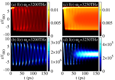
Figure 8: (Color online) Oscillations following an off-center pump pulse (in $d=1$). Panels(a,b) are for $\omega_{c}=3200$THz, where thermalization is not sufficient to suppress the oscillations. Panels (c,d) are for $\omega_{c}=3250$THz, showing a transition to a central time-independent photon cloud at late times. Panels (a,c) show $f(\mathbf{r})$, and (b,d) show $I(\mathbf{r})$. The pump pulse is a Gaussian at $r_{P}=7\ell_{\text{HO}}$, with width $\sigma_{P}=0.3\ell_{\text{HO}}$, duration duration $5$ps and intensity $\Gamma_{\uparrow}^{\text{int}}=24$GHz$\ell_{\text{HO}}$. Other parameters; $\kappa=100$MHz, $\Gamma_{\downarrow}=250$MHz, $\Gamma_{\text{max}}=3$MHz$\ell_{\text{HO}}$, mode spacing $\epsilon=0.4$THz. These last two parameters are enhanced compared to experiments to reduce simulation time. Simulations performed in one spatial dimension with $N_{m}=180$ photon modes, keeping inter-mode coherences for modes with $|m-m^{\prime}|<40$, and $N_{x}=300$ spatial grid points. This gives $~{}15,000$ coupled equations, and this requires four hours to simulate $150$ps.

Using Eq. (3,9), we simulate the dynamics following a short, high intensity, off-center pump pulse. The resulting photon density $I(\mathbf{r})$ and excited molecule fraction $f(\mathbf{r})$ are shown in Fig. 8. The behavior differs according to the cavity cutoff $\omega_{c}$ as seen experimentally Schmitt et al. (2015). Oscillations occur initially in both cases, but at late times, they are replaced by a cloud near the trap center when $\omega_{c}$ is large enough. Note that, as seen in experiment, the switch to the thermal condensate does not occur through a continuous damping of the amplitude of the oscillations, but rather through a growing intensity of the central cloud, and decaying intensity of the oscillating cloud.

As first shown by Schmitt et al. (2015), the origin of thermalization is that thermalization occurs when re-absorption of photons leads to a flat gain profile $f(\mathbf{r})\simeq f_{E}$ in the center of the trap. Our model also reproduces this behavior, as can be seen from Fig. 8(c), and is also more clearly shown in Fig. 9 which plots cross sections of $f(\mathbf{r})$ at various time slices.

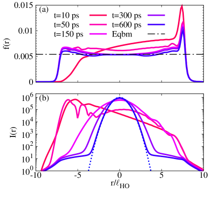
Figure 9: (Color online) Cross sections of Fig. 8, for $\omega_{c}=3250$THz. The gray dashed in panel (a) is the equilibrium population of molecules. In panel (b) the blue dashed line shows the profile of the ground mode $|\psi_{0}(r)|^{2}$.

Figure 10 shows how the photon spectrum evolves with time for $\omega_{c}=3250$THz, where oscillations disappear at late times. As also seen by Schmitt et al. (2015), the high energy modes rapidly reach a steady population, while the lower energy modes evolve more slowly, and are still evolving even after $600$ps of simulation time. Note however that the occupation of the high energy photon modes does not match the dye temperature. This is because of the limited spatial extent of the gain profile $f(\mathbf{r})$ – this extends over a range $r/\ell\lesssim 7$, so modes up to $m\lesssim 50$ will be effectively populated. This corresponds to $\omega_{m}=\omega_{c}+m\epsilon\lesssim 3270$, higher modes start to be suppressed by spatial overlap, leading to colder photon distribution, as discussed earlier.

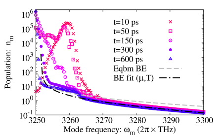
Figure 10: (Color online) Spectrum (i.e. diagonal elements of correlation matrix, $[\mathbf{n}]_{m,m}$), plotted at the same times as the cross sections in Fig. 9, plotted for $\omega_{c}=3250$THz. The black dash-dotted line in involves fitting a Bose-Einstein distribution, the fitting temperature is $175$K, and chemical potential $\mu=3251$THz — see further discussion in the text. The gray dashed line is for comparison the Bose-Einstein distribution with the Equilibrium parameters $T=300$K, $\mu=3250$THz

V Discussion and conclusions

In conclusion, we have presented a theoretical model capable of describing the spatial dynamics, relaxation, and thermalization of an inhomogeneously pumped photon condensate. Using this, we have reproduced recent experimental results studying the effects of small pump spots. Even without photon loss, thermalization can be inhibited by small spot size. Our model gives direct access to the gain profile $f(\mathbf{r})$, which is hard to access experimentally. By doing so, we see the observed behavior at and above threshold is related to gain clamping and spatial hole burning.

In this paper we have presented results only for Gaussian pump spots and harmonic trapping potentials. However, the equations we present can easily be generalized to other pump profiles or trapping potentials, e.g. ring-shaped pumps. As such, Eqs. (3,4) or the diagonal approximation, Eqs. (II.2,9), provide a useful model to predict how the spatial and spectral structure of photon condensates is determined by the properties of the pump. As well as the computation framework, some general principles can be identified from our results. Far below threshold, the condensate profile is simply given in terms of the overlaps $f_{m}$ between the pump profile and a given trap mode, allowing one to understand how the cloud will shrink if $f_{m}$ is significant only for low-order modes. A ring pump would in contrast lead to overlaps for a specific range of $m_{x},m_{y}$, and a corresponding ring-shaped thermal cloud. Far above threshold, the picture of gain saturation and spatial transverse hole burning can provide an intuitive picture of which condensate modes are favored or suppressed by a particular pump profile, and which profile shapes favor single or multimode condensation.

Mode competition and spatial pattern formation in driven dissipative systems have recently prompted significant interest in other contexts, e.g. for random lasers Türeci et al. (2008); Ge et al. (2010), where the role of mode competition and the statistics of multimode lasing have been studied. Mode competition is the basis of transverse pattern formation in nonlinear optics Denz et al. (2003); Staliunas and Sanchez-Morcillo (2003), and is a prime example of pattern formation out of equilibrium Cross and Hohenberg (1993). The model and results presented in this paper provide the foundation to study these effects in the photon condensate.

As noted in the introduction, for both lasers and condensates, order parameter equations are widely used to describe the spatial dynamics. In contrast, our work here is based on solving equations for the photon density matrix directly. By solving all elements of the photon density matrix, we allow for populations of modes in addition to the condensate mode. Such a treatment is crucial in reproducing thermal expectations, particularly below threshold. In the absence of noise terms, this is not possible with standard order parameter equations. However, thermal fluctuations can be incorporated into classical field methods by adding stochastic noise terms. This is discussed extensively in the review article by Blakie et al. (2008). It is an interesting question for future work to develop a stochastic order parameter equation that can reproduce the dynamics studied here.

As compared to work on pattern formation in polariton condensates Wertz et al. (2010); Manni et al. (2011); Tosi et al. (2012); Nelsen et al. (2013); Gao et al. (2015), an advantage of the photon condensate system is that we possess a clear model of the processes leading to the thermalization, and one which is readily tractable for spatially extended systems. For polaritons, various phenomenological models Wouters et al. (2010); Wouters (2012) have been developed, and attempts to derive models microscopically Haug et al. (2014) have been made. However questions remain open about the relative role of polariton–polariton scattering vs. scattering with phonons in the semiconductor Cao et al. (2004); Doan et al. (2005). In contrast, the models provided in this paper for the weak-coupling photon condensate are far simpler, as the effect of the (localized) ro-vibrational modes are well characterized through the function $\Gamma(\delta)$. An interesting question arising from this is to explore how to extend the treatment presented here to the case of strong coupling with organic molecules Kéna-Cohen and Forrest (2010); Plumhof et al. (2014); Daskalakis et al. (2014).

Appendix A Extracting $\Gamma(\delta)$ from experimental spectra

As discussed in section II, we aim to use the full spectrum, $\Gamma(\delta)$, extracted from experimental measurements. This spectrum includes the effects of all ro-vibrational modes automatically. The experimental measurements provide two functions $\Gamma_{\text{abs.,exp}}(\omega),\Gamma_{\text{fluor., exp}}(\omega)$, corresponding to absorption and fluoresence measurements. This appendix describes the procedure we use to find a spectrum consistent with both these measurements and the Kennard–Stepanov relation.

We first produce a single experimental function $\Gamma(\delta)$, by averaging the absorption and fluorescence measurements. This is done by identifying $\omega_{\text{ZPL}}$ from the mid-point between the peak absorption and emission, and then shifting and overlapping the experimental spectrum about these points to produce an averaged experimental function. We use a cubic-spline fit to the experimental data, and construct the function $\Gamma_{\text{exp}}(\delta)=[\Gamma_{\text{abs.,exp}}(\omega_{\text{ZPL}}+\delta)+\Gamma_{\text{fluor., exp}}(\omega_{\text{ZPL}}-\delta)]/2$. This yields a single function, but not one consistent with the Kennard–Stepanov relation. Furthermore, at large negative $\delta$, where $\Gamma_{\text{exp}}(\delta)$ is small, it falls below a noise floor, and so the experimental measurements cannot probe the exponentially small values that must be present to satisfy Kennard–Stepanov.

To address both the above points, we then construct the function:

$$\Gamma(\delta)=\frac{1+x(\delta)}{2}\Gamma_{\text{exp}}(\delta)+\frac{1-x(\delta)}{2}\Gamma_{\text{exp}}(-\delta)e^{\beta\delta},$$ (15)

where $x(\delta)$ interpolates smoothly from $-1$ at large negative $\delta$ to $+1$ at large positive $\delta$, such that $x(-\delta)=-x(\delta)$. One may readily check that this ensures $\Gamma(-\delta)e^{\beta\delta}=\Gamma(\delta)$ as required. The interpolation has the effect that we use $\Gamma(\delta)\simeq\Gamma_{\text{exp}}(\delta)$ where $\Gamma_{\text{exp}}(\delta)$ is large, and $\Gamma(\delta)\simeq\Gamma_{\text{exp}}(-\delta)e^{\beta\delta}$ where $\Gamma_{\text{exp}}(\delta)$ is small and below the noise floor, but $\Gamma_{\text{exp}}(-\delta)$ is large — see Fig. 2.

References

- Graham and Haken (1970) R. Graham and H. Haken, Z. Phys. 237, 31 (1970).
- Haken (1975) H. Haken, Rev. Mod. Phys. 47, 67 (1975).
- Staliunas and Sanchez-Morcillo (2003) K. Staliunas and V. J. Sanchez-Morcillo, Transverse Patterns in Nonlinear Optical Resonators (Springer-Verlag, Berlin, 2003).
- Kasprzak et al. (2006) J. Kasprzak, M. Richard, S. Kundermann, A. Baas, P. Jeambrun, J. M. J. Keeling, F. M. Marchetti, M. H. Szymańska, R. André, J. L. Staehli, V. Savona, P. B. Littlewood, B. Deveaud, and L. S. Dang, Nature 443, 409 (2006).
- Balili et al. (2007) R. Balili, V. Hartwell, D. Snoke, L. Pfeiffer, and K. West, Science 316, 1007 (2007).
- Carusotto and Ciuti (2013) I. Carusotto and C. Ciuti, Rev. Mod. Phys. 85, 299 (2013).
- Baumann et al. (2010) K. Baumann, C. Guerlin, F. Brennecke, and T. Esslinger, Nature 464, 1301 (2010).
- Baden et al. (2014) M. P. Baden, K. J. Arnold, A. L. Grimsmo, S. Parkins, and M. D. Barrett, Phys. Rev. Lett. 113, 020408 (2014).
- Angelakis et al. (2007) D. G. Angelakis, M. F. Santos, and S. Bose, Phys. Rev. A 76, 031805 (2007).
- Hartmann et al. (2006) M. J. Hartmann, F. G. S. L. Brandão, and M. B. Plenio, Nat. Phys. 2, 849 (2006).
- Greentree et al. (2006) A. D. Greentree, C. Tahan, J. H. Cole, and L. C. L. Hollenberg, Nat. Phys. 2, 856 (2006).
- Underwood et al. (2012) D. L. Underwood, W. E. Shanks, J. Koch, and A. A. Houck, Phys. Rev. A 86, 023837 (2012).
- Zou et al. (2014) L. J. Zou, D. Marcos, S. Diehl, S. Putz, J. Schmiedmayer, J. Majer, and P. Rabl, Phys. Rev. Lett. 113, 023603 (2014).
- Marchetti et al. (2013) M. C. Marchetti, J. F. Joanny, S. Ramaswamy, T. B. Liverpool, J. Prost, M. Rao, and R. A. Simha, Rev. Mod. Phys. 85, 1143 (2013).
- Palacci et al. (2013) J. Palacci, S. Sacanna, A. P. Steinberg, D. J. Pine, and P. M. Chaikin, Science 339, 936 (2013).
- Klaers et al. (2010a) J. Klaers, J. Schmitt, F. Vewinger, and M. Weitz, Nature 468, 545 (2010a).
- Klaers et al. (2010b) J. Klaers, F. Vewinger, and M. Weitz, Nat. Phys. 6, 512 (2010b).
- Schäfer (1990) F. P. Schäfer, ed., Dye Lasers, 3rd ed. (Springer-Verlag, 1990).
- Klaers et al. (2012) J. Klaers, J. Schmitt, T. Damm, F. Vewinger, and M. Weitz, Phys. Rev. Lett. 108, 160403 (2012).
- Sob’yanin (2012) D. N. Sob’yanin, Phys. Rev. E 85, 061120 (2012).
- Snoke and Girvin (2013) D. W. Snoke and S. M. Girvin, J. Low Temp. Phys. 171, 1 (2013).
- Kirton and Keeling (2013) P. Kirton and J. Keeling, Phys. Rev. Lett. 111, 100404 (2013).
- Kruchkov (2014) A. Kruchkov, Phys. Rev. A 89, 033862 (2014).
- van der Wurff et al. (2014) E. C. I. van der Wurff, A.-W. de Leeuw, R. A. Duine, and H. T. C. Stoof, Phys. Rev. Lett 113, 135301 (2014).
- de Leeuw et al. (2014a) A.-W. de Leeuw, H. T. C. Stoof, and R. A. Duine, Phys. Rev. A 89, 053627 (2014a).
- Chiocchetta and Carusotto (2014) A. Chiocchetta and I. Carusotto, Phys. Rev. A 90, 023633 (2014).
- Nyman and Szymańska (2014) R. A. Nyman and M. H. Szymańska, Phys. Rev. A 89, 033844 (2014).
- Sela et al. (2014) E. Sela, A. Rosch, and V. Fleurov, Phys. Rev. A 89, 043844 (2014).
- Kirton and Keeling (2015) P. Kirton and J. Keeling, Phys. Rev. A 91, 033826 (2015).
- de Leeuw et al. (2014b) A.-W. de Leeuw, E. C. I. van der Wurff, R. A. Duine, and H. T. C. Stoof, Phys. Rev. A 90, 043627 (2014b).
- Chiocchetta et al. (2015) A. Chiocchetta, A. Gambassi, and I. Carusotto, (2015), arXiv:1503.02816 .
- Schmitt et al. (2014) J. Schmitt, T. Damm, D. Dung, F. Vewinger, J. Klaers, and M. Weitz, Phys. Rev. Lett. 112, 030401 (2014).
- Marelic and Nyman (2015) J. Marelic and R. A. Nyman, Phys. Rev. A 91, 033813 (2015).
- Schmitt et al. (2015) J. Schmitt, T. Damm, D. Dung, F. Vewinger, J. Klaers, and M. Weitz, Phys. Rev. A 92, 011602 (2015).
- Wertz et al. (2010) E. Wertz, L. Ferrier, D. D. Solnyshkov, R. Johne, D. Sanvitto, A. Lemaitre, I. Sagnes, R. Grousson, A. V. Kavokin, P. Senellart, G. Malpuech, and J. Bloch, Nat. Phys. 6, 860 (2010).
- Roumpos et al. (2012) G. Roumpos, M. Lohse, W. H. Nitsche, J. Keeling, M. H. Szymanska, P. B. Littlewood, A. Löffler, S. Höfling, L. Worschech, A. Forchel, and Y. Yamamoto, Proc. Nat. Acad. Sci 109, 6467 (2012).
- Hohenberg and Halperin (1977) P. C. Hohenberg and B. I. Halperin, Rev. Mod. Phys. 49, 435 (1977).
- Sieberer et al. (2013) L. M. Sieberer, S. D. Huber, E. Altman, and S. Diehl, Phys. Rev. Lett. 110, 195301 (2013).
- Altman et al. (2015) E. Altman, L. M. Sieberer, L. Chen, S. Diehl, and J. Toner, Phys. Rev. X 5, 011017 (2015).
- (40) J. Marino and S. Diehl, arXiv:1508.02723 .
- Manni et al. (2011) F. Manni, K. G. Lagoudakis, T. C. H. Liew, R. André, and B. Deveaud-Plédran, Phys. Rev. Lett. 107, 106401 (2011).
- Tosi et al. (2012) G. Tosi, G. Christmann, N. G. Berloff, P. Tsotsis, T. Gao, Z. Hatzopoulos, P. G. Savvidis, and J. J. Baumberg, Nat. Phys. 8, 190 (2012).
- Nelsen et al. (2013) B. Nelsen, G. Liu, M. Steger, D. W. Snoke, R. Balili, K. West, and L. Pfeiffer, Phys. Rev. X 3, 041015 (2013).
- Gao et al. (2015) T. Gao, E. Estrecho, K. Y. Bliokh, T. C. H. Liew, M. D. Fraser, S. Brodbeck, M. Kamp, C. Schneider, S. Höfling, Y. Yamamoto, F. Nori, Y. S. Kivshar, A. G. Truscott, R. G. Dall, and E. A. Ostrovskaya, Nature 526, 554 (2015).
- Kollár et al. (2015) A. J. Kollár, A. T. Papageorge, K. Baumann, M. A. Armen, and B. L. Lev, New J. Phys. 17, 043012 (2015).
- Pitaevskii and Stringari (2003) L. P. Pitaevskii and S. Stringari, Bose-Einstein Condensation (Clarendon Press, Oxford, 2003).
- Ginzburg and Landau (1950) V. L. Ginzburg and L. D. Landau, Zh. Eksp. Teor. Fiz 20, 1064 (1950).
- Aranson and Kramer (2002) I. Aranson and L. Kramer, Rev. Mod. Phys. 74, 99 (2002).
- Wouters and Carusotto (2007) M. Wouters and I. Carusotto, Phys. Rev. Lett. 99, 140402 (2007).
- Keeling and Berloff (2008) J. Keeling and N. G. Berloff, Phys. Rev. Lett. 100, 250401 (2008).
- Wouters et al. (2008) M. Wouters, I. Carusotto, and C. Ciuti, Phys. Rev. B 77, 115340 (2008).
- Wouters et al. (2010) M. Wouters, T. C. H. Liew, and V. Savona, Phys. Rev. B 82, 245315 (2010).
- Wouters (2012) M. Wouters, New J. Phys. 14, 075020 (2012).
- (54) R. A. Nyman and J. Marelic, Private Communication. The absorption spectrum is a composite at several concentrations, to improve the accuracy around 3200 THz.
- Kennard (1918) E. H. Kennard, Phys. Rev. 11, 29 (1918).
- Kennard (1926) E. H. Kennard, Phys. Rev. 28, 672 (1926).
- Stepanov (1957) B. I. Stepanov, Dokl. Akad. Nauk SSR 112, 839 (1957).
- Dümcke and Spohn (1979) R. Dümcke and H. Spohn, Zeitschrift fur Phys. B 34, 419 (1979).
- Jeske et al. (2015) J. Jeske, D. Ing, M. B. Plenio, S. F. Huelga, and J. H. Cole, J. Chem. Phys. 142, 064104 (2015).
- Joshi et al. (2014) C. Joshi, P. Ohberg, J. D. Cresser, and E. Andersson, Phys. Rev. A 90, 063815 (2014).
- (61) P. Eastham, P. Kirton, H. Cammack, B. W. Lovett, and J. Keeling, “Bath induced coherence and the secular approximation,” Submitted, arXiv:1508.04744 .
- Marthaler et al. (2011) M. Marthaler, Y. Utsumi, D. S. Golubev, A. Shnirman, and G. Schön, Phys. Rev. Lett. 107, 093901 (2011).
- Siegman (1986) A. E. Siegman, Lasers (University Science Books, Sausolito, 1986).
- Türeci et al. (2008) H. E. Türeci, A. D. Stone, L. Ge, S. Rotter, and R. J. Tandy, Nonlinearity 22, C1 (2008).
- Ge et al. (2010) L. Ge, Y. D. Chong, and A. D. Stone, Phys. Rev. A 82, 063824 (2010).
- Denz et al. (2003) C. Denz, M. Schwab, and C. Weilnau, Transverse-Pattern Formation in Photorefractive Optics, Springer Tracts in Modern Physics, Vol. 188 (Springer-Verlag, Berlin, 2003).
- Cross and Hohenberg (1993) M. C. Cross and P. C. Hohenberg, Rev. Mod. Phys. 65, 851 (1993).
- Blakie et al. (2008) P. B. Blakie, A. S. Bradley, M. J. Davis, R. J. Ballagh, and C. W. Gardiner, Adv. Phys. 57, 363 (2008).
- Haug et al. (2014) H. Haug, T. D. Doan, and D. B. Tran Thoai, Phys. Rev. B 89, 155302 (2014).
- Cao et al. (2004) H. T. Cao, T. D. Doan, D. B. Tran Thoai, and H. Haug, Phys. Rev. B 69, 245325 (2004).
- Doan et al. (2005) T. D. Doan, H. T. Cao, D. B. Tran Thoai, and H. Haug, Phys. Rev. B 72, 085301 (2005).
- Kéna-Cohen and Forrest (2010) S. Kéna-Cohen and S. R. Forrest, Nat. Photon. 4, 371 (2010).
- Plumhof et al. (2014) J. D. Plumhof, T. Stöferle, L. Mai, U. Scherf, and R. F. Mahrt, Nat. Mater. 13, 247 (2014).
- Daskalakis et al. (2014) K. S. Daskalakis, S. A. Maier, R. Murray, and S. Kéna-Cohen, Nat. Mater. 13, 271 (2014).