Diversity in Spectral Learning for Natural Language Parsing

Abstract

We describe an approach to create a diverse set of predictions with spectral learning of latent-variable PCFGs (L-PCFGs). Our approach works by creating multiple spectral models where noise is added to the underlying features in the training set before the estimation of each model. We describe three ways to decode with multiple models. In addition, we describe a simple variant of the spectral algorithm for L-PCFGs that is fast and leads to compact models. Our experiments for natural language parsing, for English and German, show that we get a significant improvement over baselines comparable to state of the art. For English, we achieve the $F_{1}$ score of 90.18, and for German we achieve the $F_{1}$ score of 83.38.

1 Introduction

It has been long identified in NLP that a diverse set of solutions from a decoder can be reranked or recombined in order to improve the accuracy in various problems [Henderson and Brill, 1999]. Such problems include machine translation [Macherey and Och, 2007], syntactic parsing [Charniak and Johnson, 2005, Sagae and Lavie, 2006, Fossum and Knight, 2009, Zhang et al., 2009, Petrov, 2010, Choe et al., 2015] and others [Van Halteren et al., 2001].

The main argument behind the use of such a diverse set of solutions (such as $k$-best list of parses for a natural language sentence) is the hope that each solution in the set is mostly correct. Therefore, recombination or reranking of solutions in that set will further optimize the choice of a solution, combining together the information from all solutions.

In this paper, we explore another angle for the use of a set of parse tree predictions, where all predictions are made for the same sentence. More specifically, we describe techniques to exploit diversity with spectral learning algorithms for natural language parsing. Spectral techniques and the method of moments have been recently used for various problems in natural language processing, including parsing, topic modeling and the derivation of word embeddings [Luque et al., 2012, Cohen et al., 2013, Stratos et al., 2014, Dhillon et al., 2015, Rastogi et al., 2015, Nguyen et al., 2015, Lu et al., 2015].

?) showed how to estimate an L-PCFG using spectral techniques, and showed that such estimation outperforms the expectation-maximization algorithm [Matsuzaki et al., 2005]. Their result still lags behind state of the art in natural language parsing, with methods such as coarse-to-fine [Petrov et al., 2006].

We further advance the accuracy of natural language parsing with spectral techniques and L-PCFGs, yielding a result that outperforms the original Berkeley parser from ?). Instead of exploiting diversity from a $k$-best list from a single model, we estimate multiple models, where the underlying features are perturbed with several perturbation schemes. Each such model, during test time, yields a single parse, and all parses are then used together in several ways to select a single best parse.

The main contributions of this paper are two-fold. First, we present an algorithm for estimating L-PCFGs, akin to the spectral algorithm of ?), but simpler to understand and implement. This algorithm has value for readers who are interested in learning more about spectral algorithms – it demonstrates some of the core ideas in spectral learning in a rather intuitive way. In addition, this algorithm leads to sparse grammar estimates and compact models.

Second, we describe how a diverse set of predictors can be used with spectral learning techniques. Our approach relies on adding noise to the feature functions that help the spectral algorithm compute the latent states. Our noise schemes are similar to those described by ?). We add noise to the whole training data, then train a model using our algorithm (or other spectral algorithms; Cohen et al., 2013), and repeat this process multiple times. We then use the set of parses we get from all models in a recombination step.

The rest of the paper is organized as follows. In §2 we describe notation and background about L-PCFG parsing. In §3 we describe our new spectral algorithm for estimating L-PCFGs. It is based on similar intuitions as older spectral algorithms for L-PCFGs. In §4 we describe the various noise schemes we use with our spectral algorithm and the spectral algorithm of ?). In §5 we describe how to decode with multiple models, each arising from a different noise setting. In §6 we describe our experiments with natural language parsing for English and German.

2 Background and Notation

We denote by $[n]$ the set of integers $\{1,\ldots,n\}$. For a statement $\Gamma$, we denote by $[[\Gamma]]$ its indicator function, with values 0 when the assertion is false and 1 when it is true.

An L-PCFG is a 5-tuple $({\cal N},{\cal I},{\cal P},m,n)$ where:

• ${\cal N}$ is the set of nonterminal symbols in the grammar. ${\cal I}\subset{\cal N}$ is a finite set of interminals. ${\cal P}\subset{\cal N}$ is a finite set of preterminals. We assume that ${\cal N}={\cal I}\cup{\cal P}$, and ${\cal I}\cap{\cal P}=\emptyset$. Hence we have partitioned the set of nonterminals into two subsets.

• $[m]$ is the set of possible hidden states.

• $[n]$ is the set of possible words.

• For all $a\in{\cal I}$, $b\in{\cal N}$, $c\in{\cal N}$, $h_{1},h_{2},h_{3}\in[m]$, we have a binary context-free rule $a(h_{1})\rightarrow b(h_{2})\;\;c(h_{3})$.

• For all $a\in{\cal P}$, $h\in[m]$, $x\in[n]$, we have a lexical context-free rule $a(h)\rightarrow x$.

Latent-variable PCFGs are essentially equivalent to probabilistic regular tree grammars (PRTGs; Knight and Graehl, 2005) where the righthand side trees are of depth 1. With general PRTGs, the righthand side can be of arbitrary depth, where the leaf nodes of these trees correspond to latent states in the L-PCFG formulation above and the internal nodes of these trees correspond to interminal symbols in the L-PCFG formulation.

Two important concepts that will be used throughout of the paper are that of an “inside tree” and an “outside tree.” Given a tree, the inside tree for a node contains the entire subtree below that node; the outside tree contains everything in the tree excluding the inside tree. See Figure 1 for an example. Given a grammar, we denote the space of inside trees by $T$ and the space of outside trees by $O$.

[.VP [.V saw ] [.NP [.D the ] [.N woman ] ] ]

[.S [.NP [.D the ] [.N dog ] ] VP ]

Figure 1: The inside tree (left) and outside tree (right) for the nonterminal VP in the parse tree (S (NP (D the) (N dog)) (VP (V saw) (NP (D the) (N woman)))).

Inputs: An input treebank with the following additional information: training examples $(a^{(i)},t^{(i)},o^{(i)},b^{(i)})$ for $i\in\{1\ldots M\}$, where $a^{(i)}\in{\cal N}$; $t^{(i)}$ is an inside tree; $o^{(i)}$ is an outside tree; and $b^{(i)}=1$ if the rule is at the root of tree, $0$ otherwise. A function $\phi$ that maps inside trees $t$ to feature-vectors $\phi(t)\in\mbox{\msym R}^{d}$. A function $\psi$ that maps outside trees $o$ to feature-vectors $\psi(o)\in\mbox{\msym R}^{d^{\prime}}$. An integer $k$ denoting the thin-SVD rank. An integer $m$ denoting the number of latent states.   Algorithm: (Step 1: Singular Value Decompositions) • Calculate SVD on $\Omega^{a}$ to get $\hat{U}^{a}\in\mbox{\msym R}^{(d\times k)}$ and $\hat{V}^{a}\in\mbox{\msym R}^{(d^{\prime}\times k)}$ for each $a\in{\cal N}$. (Step 1: Projection) • For all $i\in[M]$, compute $y^{(i)}=(\hat{U}^{a_{i}})^{\top}\phi(t^{(i)})$ and $z^{(i)}=(\hat{V}^{a_{i}})^{\top}\psi(o^{(i)})$. • For all $i\in[M]$, set $x^{(i)}$ to be the concatenation of $y^{(i)}$ and $z^{(i)}$. (Step 2: Cluster Projections) • For all $a\in{\cal N}$, cluster the set $\{x^{(i)}\mid a^{(i)}=a\}$ to get a clustering function $\gamma\colon\mbox{\msym R}^{2k}\rightarrow[m]$ that maps a projected vector $x^{(i)}$ to a cluster in $[m]$. (Step 3: Compute Final Parameters) • Annotate each node in the treebank with $\gamma(x^{(i)})$. • Compute the probability of a rule $p(a[h_{1}]\rightarrow b[h_{2}]\,c[h_{3}]\mid a[h_{1}])$ as the relative frequency of its appearance in the cluster-annotated treebank. • Similarly, compute the root probabilities $\pi(a[h])$ and preterminal rules $p(a[h]\rightarrow x\mid a[h])$.

Figure 2: The clustering estimation algorithm for L-PCFGs.

3 Clustering Algorithm for Estimating L-PCFGs

We assume two feature functions, $\phi\colon T\rightarrow\mbox{\msym R}^{d}$ and $\psi\colon O\rightarrow\mbox{\msym R}^{d^{\prime}}$, mapping inside and outside trees, respectively, to a real vector. Our training data consist of examples $(a^{(i)},t^{(i)},o^{(i)},b^{(i)})$ for $i\in\{1\ldots M\}$, where $a^{(i)}\in{\cal N}$; $t^{(i)}$ is an inside tree; $o^{(i)}$ is an outside tree; and $b^{(i)}=1$ if $a^{(i)}$ is the root of tree, $0$ otherwise. These are obtained by splitting all trees in the training set into inside and outside trees at each node in each tree. We then define $\Omega^{a}\in\mbox{\msym R}^{d\times d^{\prime}}$:

$$\Omega^{a}=\frac{\sum_{i=1}^{M}[[a^{(i)}=a]]\phi(t^{(i)})(\psi(o^{(i)}))^{\top}}{\sum_{i=1}^{M}[[a^{(i)}=a]]}$$ (1)

This matrix is an empirical estimate for the cross-covariance matrix between the inside trees and the outside trees of a given nonterminal $a$. An inside tree and an outside tree are conditionally independent according to the L-PCFG model, when the latent state at their connecting point is known. This means that the latent state can be identified by finding patterns that co-occur together in inside and outside trees – it is the only random variable that can explain such correlations. As such, if we reduce the dimensions of $\Omega^{a}$ using singular value decomposition (SVD), we essentially get representations for the inside trees and the outside trees that correspond to the latent states.

This intuition leads to the algorithm that appears in Figure 2. The algorithm we describe takes as input training data, in the form of a treebank, decomposed into inside and outside trees at each node in each tree in the training set.

The algorithm first performs SVD for each of the set of inside and outside trees for all nonterminals. This step is akin to CCA, which has been used in various contexts in NLP, mostly to derive representations for words [Dhillon et al., 2015, Rastogi et al., 2015]. The algorithm then takes the representations induced by the SVD step, and clusters them – we use $k$-means to do the clustering. Finally, it maps each SVD representation to a cluster, and as a result, gets a cluster identifier for each node in each tree in the training data. These clusters are now treated as latent states that are “observed.” We subsequently follow up with frequency count maximum likelihood estimate to estimate the probabilities of each parameter in the L-PCFG.

Consider for example the estimation of rules of the form $a\rightarrow x$. Following the clustering step we obtain for each nonterminal $a$ and latent state $h$ a set of rules of the form $a[h]\rightarrow x$. Each such instance comes from a single training example of a lexical rule. Next, we compute the probability of the rule $a[h]\rightarrow x$ by counting how many times that rule appears in the training instances, and normalize by the total count of $a[h]$ in the training instances. Similarly, we compute probabilities for binary rules of the form $a\rightarrow b\,c$.

The features that we use for $\phi$ and $\psi$ are similar to those used in ?). These features look at the local neighborhood surrounding a given node. More specifically, we indicate the following information with the inside features (throughout these definitions assume that $a\rightarrow b\,c$ is at the root of the inside tree $t$):

• The pair of nonterminals $(a,b)$. E.g., for the inside tree in Figure 1 this would be the pair (VP, V).

• The pair $(a,c)$. E.g., (VP, NP).

• The rule $a\rightarrow b\,c$. E.g., VP $\rightarrow$ V NP.

• The rule $a\rightarrow b\,c$ paired with the rule at the node $b$. E.g., for the inside tree in Figure 1 this would correspond to the tree fragment (VP (V saw) NP).

• The rule $a\rightarrow b\,c$ paired with the rule at the node $c$. E.g., the tree fragment (VP V (NP D N)).

• The head part-of-speech of $t$ paired with $a$. E.g., the pair (VP, V).

• The number of words dominated by $t$ paired with $a$. E.g., the pair (VP, 3).

In the case of an inside tree consisting of a single rule $a\rightarrow x$ the feature vector simply indicates the identity of that rule.

For the outside features, we use:

• The rule above the foot node. E.g., for the outside tree in Figure 1 this would be the rule S $\rightarrow$ NP VP^∗ (the foot nonterminal is marked with $*$).

• The two-level and three-level rule fragments above the foot node. These features are absent in the outside tree in Figure 1.

• The label of the foot node, together with the label of its parent. E.g., the pair (VP, S).

• The label of the foot node, together with the label of its parent and grandparent.

• The part-of-speech of the first head word along the path from the foot of the outside tree to the root of the tree which is different from the head node of the foot node.

• The width of the spans to the left and to the right of the foot node, paired with the label of the foot node.

Other Spectral Algorithms

The SVD step on the $\Omega^{a}$ matrix is pivotal to many algorithms, and has been used in the past for other L-PCFG estimation algorithms. ?) used it for developing a spectral algorithm that identifies the parameters of the L-PCFG up to a linear transformation. Their algorithm generalizes the work of ?) and ?).

?) also developed an algorithm that makes use of an SVD step on the inside-outside. It relies on the idea of “pivot features” – features that uniquely identify latent states.

?) used a clustering algorithm that resembles ours but does not separate inside trees from outside trees or follows up with a singular value decomposition step. Their algorithm was applied to both L-PCFGs and linear context-free rewriting systems. Their application was the analysis of hierarchical structure of conversations in online forums.

In our preliminary experiments, we found out that the clustering algorithm by itself performs worse than the spectral algorithm of ?). We believe that the reason is two-fold: (a) $k$-means finds a local maximum during clustering; (b) we do hard clustering instead of soft clustering. However, we detected that the clustering algorithm gives a more diverse set of solutions, when the features are perturbed. As such, in the next sections, we explain how to perturb the models we get from the clustering algorithm (and the spectral algorithm) in order to improve the accuracy of the clustering and spectral algorithms.

4 Spectral Estimation with Noise

It has been shown that a diverse set of predictions can be used to help improve decoder accuracy for various problems in NLP [Henderson and Brill, 1999]. Usually a $k$-best list from a single model is used to exploit model diversity. Instead, we estimate multiple models, where the underlying features are filtered with various noising schemes.

We try three different types of noise schemes for the algorithm in Figure 2:

Dropout noise:

Let $\sigma\in[0,1]$. We set each element in the feature vectors $\phi(t)$ and $\psi(o)$ to $0$ with probability $\sigma$.

Gaussian (additive):

Let $\sigma>0$. For each $x^{(i)}$, we draw a vector $\varepsilon\in\mbox{\msym R}^{2k}$ of Gaussians with mean 0 and variance $\sigma^{2}$, and then set $x^{(i)}\leftarrow x^{(i)}+\varepsilon$.

Gaussian (multiplicative):

Let $\sigma>0$. For each $x^{(i)}$, we draw a vector $\varepsilon\in\mbox{\msym R}^{2k}$ of Gaussians with mean 0 and variance $\sigma^{2}$, and then set $x^{(i)}\leftarrow x^{(i)}\otimes(1+\varepsilon)$, where $\otimes$ is coordinate-wise multiplication.

Note the distinction between the dropout noise and the Gaussian noise schemes: the first is performed on the feature vectors before the SVD step, and the second is performed after the SVD step. It is not feasible to add Gaussian noise prior to the SVD step, since the matrix $\Omega^{a}$ will no longer be sparse, and its SVD computation will be computationally demanding.

Our use of dropout noise here is inspired by “dropout” as is used in neural network training, where various connections between units in the neural network are dropped during training in order to avoid overfitting of these units to the data [Srivastava et al., 2014].

The three schemes we described were also used by ?) to train log-linear models. Wang et al.’s goal was to prevent overfitting by introducing this noise schemes as additional regularizer terms, but without explicitly changing the training data. We do filter the data through these noise schemes, and show in §6 that all of these noise schemes do not improve the performance of our estimation on their own. However, when multiple models are created with these noise schemes, and then combined together, we get an improved performance. As such, our approach is related to the one of ?), who builds a committee of latent-variable PCFGs in order to improve a natural language parser.

We also use these perturbation schemes to create multiple models for the algorithm of ?). The dropout scheme stays the same, but for the Gaussian noising schemes, we follow a slightly different procedure. After noising the projections of the inside and outside feature functions we get from the SVD step, we use these projected noised features as a new set of inside and outside feature functions, and re-run the spectral algorithm of ?) on them.

We are required to add this extra SVD step because the spectral algorithm of Cohen et al. assumes the existence of linearly transformed parameter estimates, where the parameters of each nonterminal $a$ is linearly transformed by unknown invertible matrices. These matrices cancel out when the inside-outside algorithm is run with the spectral estimate output. In order to ensure that these matrices still exactly cancel out, we have to follow with another SVD step as described above. The latter SVD step is performed on a dense $\Omega^{a}\in\mbox{\msym R}^{m\times m}$ but this is not an issue considering $m$ (the number of latent states) is much smaller than $d$ or $d^{\prime}$.

5 Decoding with Multiple Models

Let $G_{1},\ldots,G_{p}$ be a set of L-PCFG grammars. In §6, we create such models using the noising techniques described above. The question that remains is how to combine these models together to get a single best output parse tree given an input sentence.

With L-PCFGs, decoding a single sentence requires marginalizing out the latent states to find the best skeletal tree for a given string. Let $s$ be a sentence. We define $t(G_{i},s)$ to be the output tree according to minimum Bayes risk decoding. This means we follow ?), who uses dynamic programming to compute the tree that maximizes the sum of all marginals of all nonterminals in the output tree. Each marginal, for each span $\langle a,i,j\rangle$ (where $a$ is a nonterminal and $i$ and $j$ are endpoints in the sentence), is computed by using the inside-outside algorithm.

In addition, let $\mu(a,i,j|G_{k},s)$ be the marginal, as computed by the inside-outside algorithm, for the span $\langle a,i,j\rangle$ with grammar $G_{k}$ for string $s$. We use the notation $\langle a,i,j\rangle\in t$ to denote that a span $\langle a,i,j\rangle$ is in a tree $t$.

We suggest the following three ways for decoding with multiple models $G_{1},\ldots,G_{p}$:

Maximal tree coverage:

Using dynamic programming, we return the tree that is the solution to:

$$t^{\ast}=\arg\max_{t}\sum_{\langle a,i,j\rangle\in t}\sum_{k=1}^{p}[[\langle a,i,j\rangle\in t(G_{k},s)]].$$

This implies that we find the tree that maximizes its coverage with respect to all other trees that are decoded using $G_{1},\ldots,G_{p}$.

Maximal marginal coverage:

Using dynamic programming, we return the tree that is the solution to:

$$t^{\ast}=\arg\max_{t}\sum_{\langle a,i,j\rangle\in t}\sum_{k=1}^{p}\mu(a,i,j|G_{k},s).$$

This is similar to maximal tree coverage, only instead of considering just the single decoded tree for each model among $G_{1},\ldots,G_{p}$, we make our decoding “softer,” and rely on the marginals that each model gives.

MaxEnt reranking:

We train a MaxEnt reranker on a training set that includes outputs from multiple models, and then, during testing time, decode with each of the models, and use the trained reranker to select one of the parses. We use the reranker of ?).

As we see later in §6, it is sometimes possible to extract more information from the training data by using a network, or a hierarchy of the above tree combination methods. For example, we get our best result for parsing by first using MaxEnt with several subsets of the models, and then combining the output of these MaxEnt models using maximal tree coverage.

6 Experiments

In this section, we describe parsing experiments with two languages: English and German.

6.1 Results for English

	Clustering			Spectral (smoothing)			Spectral (no smoothing)
	MaxTre	MaxMrg	MaxEnt	MaxTre	MaxMrg	MaxEnt	MaxTre	MaxMrg	MaxEnt
Add	88.68	88.64	89.50	88.20	88.28	88.59	86.72	86.85	87.94
Mul	88.74	88.66	89.89	88.48	88.70	89.46	86.97	86.53	89.04
Dropout	88.68	88.56	89.80	88.64	88.71	89.47	88.37	88.06	89.52
All	88.84	88.75	89.95	88.38	88.75	89.45	87.49	87.00	89.85
No noise	86.48			88.53 (Cohen et al., 2013)			86.47 (Cohen et al., 2013)

Table 1: Results on section 22 (WSJ). MaxTre denotes decoding using maximal tree coverage, MaxMrg denotes decoding using maximal marginal coverage, and MaxEnt denotes the use of a discriminative reranker. Add, Mul  and Dropout  denote the use of additive Gaussian noise, multiplicative Gaussian noise and dropout noise, respectively. The number of models used in the first three rows for the clustering algorithm is 80: 20 for each $\sigma\in\{0.05,0.1,0.15,0.2\}$. For the spectral algorithm, it is 20, 5 for each $\sigma$ (see footnotes). The number of latent states is $m=24$. For All, we use all models combined from the first three rows. The “No noise” baseline for the spectral algorithm is taken from Cohen et al. (2013). The best figure in each algorithm block is in boldface.

For our English parsing experiments, we use a standard setup. More specifically, we use the Penn WSJ treebank [Marcus et al., 1993] for our experiments, with sections 2–21 as the training data, and section 22 used as the development data. Section 23 is used as the final test set. We binarize the trees in training data, but transform them back before evaluating them.

For efficiency, we use a base PCFG without latent states to prune marginals which receive a value less than $0.00005$ in the dynamic programming chart. The parser takes part-of-speech tagged sentences as input. We tag all datasets using Turbo Tagger [Martins et al., 2010], trained on sections 2–21. We use the $F_{1}$ measure according to the PARSEVAL metric [Black et al., 1991] for the evaluation.

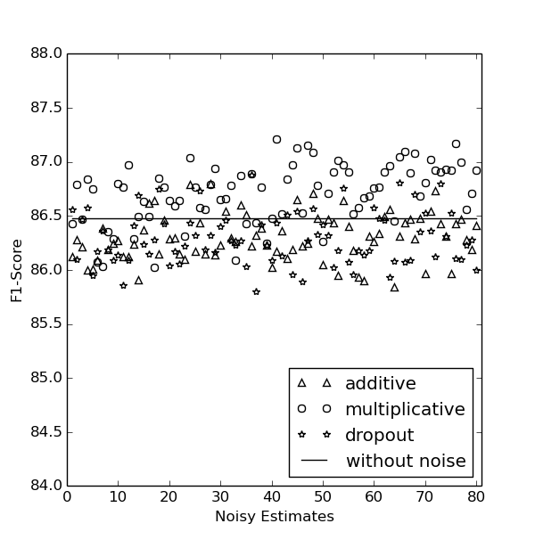
Figure 3: $F_{1}$ scores of noisy models. Each data point gives the $F_{1}$ accuracy of a single model on the development set, based on the legend. The $x$-axis enumerates the models (80 in total for each noise scheme).

Preliminary experiments

We first experiment with the number of latent states for the clustering algorithm without perturbations. We use $k=100$ for the SVD step. Whenever we need to cluster a set of points, we run the $k$-means algorithm $10$ times with random restarts and choose the clustering result with the lowest objective value. On section 22, the clustering algorithm achieves the following results ($F_{1}$ measure): $m=8$: 84.30%, $m=16$: 85.98%, $m=24$: 86.48%, $m=32$: 85.84%, $m=36$: 86.05%, $m=40$: 85.43%. As we increase the number of states, performance improves, but plateaus at $m=24$. For the rest of our experiments, both with the spectral algorithm of ?) and the clustering algorithm presented in this paper, we use $m=24$.

Compact models

One of the advantage of the clustering algorithm is that it leads to much more compact models. The number of nonzero parameters with $m=24$ for the clustering algorithm is approximately 97K, while the spectral algorithms lead to a significantly larger number of nonzero parameters with the same number of latent states: approximately 54 million.

	Method	$F_{1}$
Best	Spectral (unsmoothed)	89.21
	Spectral (smoothed)	88.87
	Clustering	89.25
Hier	Spectral (unsmoothed)	89.09
	Spectral (smoothed)	89.06
	Clustering	90.18

Table 2: Results on section 23 (English). The first three results (Best) are taken with the best model in each corresponding block in Table 1. The last three results (Hier) use a hierarchy of the above tree combination methods in each block. It combines all MaxEnt results using the maximal tree coverage (see text).

Oracle experiments

To what extent do we get a diverse set of solutions from the different models we estimate? This question can be answered by testing the oracle accuracy in the different settings. For each type of noising scheme, we generated 80 models, 20 for each $\sigma\in\{0.05,0.1,0.15,0.2\}$. Each noisy model by itself lags behind the best model (see Figure 3). However, when choosing the best tree among these models, the additively-noised models get an oracle accuracy of 95.91% on section 22; the multiplicatively-noised models get an oracle accuracy of 95.81%; and the dropout-noised models get an oracle accuracy of 96.03%. Finally all models combined get an oracle accuracy of 96.67%. We found out that these oracle scores are comparable to the one ?) report.

We also tested our oracle results, comparing the spectral algorithm of ?) to the clustering algorithm. We generated 20 models for each type of noising scheme, 5 for each $\sigma\in\{0.05,0.1,0.15,0.2\}$) for the spectral algorithm. Surprisingly, even though the spectral models were smoothed, their oracle accuracy was lower than the accuracy of the clustering algorithm: 92.81% vs. 95.73%. This reinforces two ideas: (i) that noising acts as a regularizer, and has a similar role to backoff smoothing, as we see below; and (ii) the noisy estimation for the clustering algorithm produces a more diverse set of parses than that produced with the spectral algorithm.

It is also important to note that the high oracle accuracy is not just the result of $k$-means not finding the global maximum for the clustering objective. If we just run the clustering algorithms with 80 models as before, without perturbing the features, the oracle accuracy is 95.82%, which is lower than the oracle accuracy with the additive and dropout perturbed models. To add to this, we see below that perturbing the training set with the spectral algorithm of Cohen et al. improves the accuracy of the spectral algorithm. Since the spectral algorithm of Cohen et al. does not maximize any objective locally, it shows that the role of the perturbations we use is important.

	Clustering			Spectral (smoothing)			Spectral (no smoothing)
	MaxTre	MaxMrg	MaxEnt	MaxTre	MaxMrg	MaxEnt	MaxTre	MaxMrg	MaxEnt
Add	77.34	76.87	80.01	77.76	77.85	78.09	77.44	77.56	77.91
Mul	77.80	77.80	80.34	77.80	77.76	78.89	77.62	77.85	78.94
Dropout	77.37	77.17	80.94	77.94	78.06	79.02	77.97	78.17	79.18
All	77.71	77.51	80.86	78.04	77.89	79.46	77.73	77.91	79.66
No noise	75.04			77.71			77.07

Table 3: Results on the development set for German. See Table 1 for interpretation of MaxTre, MaxMrg, MaxEnt and Add, Mul  and Dropout. The number of models used in the first three rows for the clustering algorithm is 80: 20 for each $\sigma\in\{0.05,0.1,0.15,0.2\}$. For the spectral algorithm, it is 20, 5 for each $\sigma$. The number of latent states is $m=8$. For All, we use all models combined from the first three rows. The best figure in each algorithm block is in boldface.

Results

Results on the development set are given in Table 1 with our three decoding methods. We present the results from three algorithms: the clustering algorithm and the spectral algorithms (smoothed and unsmoothed).

It seems that dropout noise for the spectral algorithm acts as a regularizer, similarly to the backoff smoothing techniques that are used in ?). This is evident from the two spectral algorithm blocks in Table 1, where dropout noise does not substantially improve the smoothed spectral model (Cohen et al. report accuracy of 88.53% with smoothed spectral model for $m=24$ without noise) – the accuracy is 88.64%–88.71%–89.47%, but the accuracy substantially improves for the unsmoothed spectral model, where dropout brings an accuracy of 86.47% up to 89.52%.

All three blocks in Table 1 demonstrate that decoding with the MaxEnt reranker performs the best. Also it is interesting to note that our results continue to improve when combining the output of previous combination steps further. The best result on section 22 is achieved when we combine, using maximal tree coverage, all MaxEnt outputs of the clustering algorithm (the first block in Table 1). This yields a 90.68% $F_{1}$ accuracy. This is also the best result we get on the test set (section 23), 90.18%. See Table 2 for results on section 23.

Our results are comparable to state-of-the-art results for parsing. For example, ?), ?) and ?) report an accuracy of 93.2%-93.3% using parsing recombination; ?) report an accuracy of 92.4 $F_{1}$ using a Bayesian tree substitution grammar; ?) reports an accuracy of 92.0% using product of L-PCFGs; ?) report accuracy of 91.4 using a discriminative reranking model; ?) report 91.1 $F_{1}$ accuracy for a discriminative, perceptron-trained model; ?) report an accuracy of 90.1 $F_{1}$. ?) reports an accuracy of 88.2 $F_{1}$.

6.2 Results for German

For the German experiments, we used the NEGRA corpus [Skut et al., 1997]. We use the same setup as in ?), and use the first 18,602 sentences as a training set, the next 1,000 sentences as a development set and the last 1,000 sentences as a test set. This corresponds to an 80%-10%-10% split of the treebank.

Our German experiments follow the same setting as in our English experiments. For the clustering algorithm we generated 80 models, 20 for each $\sigma\in\{0.05,0.1,0.15,0.2\}$. For the spectral algorithm, we generate 20 models, 5 for each $\sigma$.

For the reranking experiment, we had to modify the BLLIP parser [Charniak and Johnson, 2005] to use the head features from the German treebank. We based our modifications on the documentation for the NEGRA corpus (our modifications are based mostly on mapping of nonterminals to coarse syntactic categories).

Preliminary experiments

For German, we also experiment with the number of latent states. On the development set, we observe that the $F_{1}$ measure is: 75.04% for $m=8$, 73.44% for $m=16$ and 70.84% for $m=24$. For the rest of our experiments, we fix the number of latent states at $m=8$.

	Method	$F_{1}$
Best	Spectral (unsmoothed)	80.88
	Spectral (smoothed)	80.31
	Clustering	81.94
Hier	Spectral (unsmoothed)	80.64
	Spectral (smoothed)	79.96
	Clustering	83.38

Table 4: Results on the test set for the German data. The first three results (Best) are taken with the best model in each corresponding block in Table 3. The last three results (Hier) use a hierarchy of the above tree combination methods.

Oracle experiments

The additively-noised models get an oracle accuracy of 90.58% on the development set; the multiplicatively-noised models get an oracle accuracy of 90.47%; and the dropout-noised models get an oracle accuracy of 90.69%. Finally all models combined get an oracle accuracy of 92.38%.

We compared our oracle results to those given by the spectral algorithm of ?). With 20 models for each type of noising scheme, all spectral models combined achieve an oracle accuracy of 83.45%. The clustering algorithm gets the oracle score of 90.12% when using the same number of models.

Results

Results on the development set and on the test set are given in Table 3 and Table 4 respectively.

Like English, in all three blocks in Table 3, decoding with the MaxEnt reranking performs the best. Our results continue to improve when further combining the output of previous combination steps. The best result of 82.04% on the development set is achieved when we combine, using maximal tree coverage, all MaxEnt outputs of the clustering algorithm (the first block in Table 3). This also leads to the best result of 83.38% on the test set. See Table 4 for results on the test set.

Our results are comparable to state-of-the-art results for German parsing. For example, ?) reports an accuracy of 84.5% using product of L-PCFGs; ?) report an accuracy of 80.1 $F_{1}$; and ?) reports an accuracy of 76.3 $F_{1}$.

7 Discussion

From a theoretical point of view, one of the great advantages of spectral learning techniques for latent-variable models is that they yield consistent parameter estimates. Our clustering algorithm for L-PCFG estimation breaks this, but there is a work-around to obtain an algorithm which would be statistically consistent.

The main reason that our algorithm is not a consistent estimator is that it relies on $k$-means clustering, which maximizes a non-convex objective using hard clustering steps. The $k$-means algorithm can be viewed as “hard EM” for a Gaussian mixture model (GMM), where each latent state is associated with one of the mixture components in the GMM. This means that instead of following up with $k$-means, we could have identified the parameters and the posteriors for a GMM, where the observations correspond to the vectors that we cluster. There are now algorithms, some of which are spectral, that aim to solve this estimation problem with theoretical guarantees [Vempala and Wang, 2004, Kannan et al., 2005, Moitra and Valiant, 2010].

With theoretical guarantees on the correctness of the posteriors from this step, the subsequent use of maximum likelihood estimation step could yield consistent parameter estimates. The consistency guarantees will largely depend on the amount of information that exists in the base feature functions about the latent states according to the L-PCFG model.

8 Conclusion

We presented a novel estimation algorithm for latent-variable PCFGs. This algorithm is based on clustering of continuous tree representations, and it also leads to sparse grammar estimates and compact models. We also showed how to get a diverse set of parse tree predictions with this algorithm and also older spectral algorithms. Each prediction in the set is made by training an L-PCFG model after perturbing the underlying features that estimation algorithm uses from the training data. We showed that such a diverse set of predictions can be used to improve the parsing accuracy of English and German.

References

- [Bailly et al., 2010] Raphaël Bailly, Amaury Habrard, and François Denis. 2010. A spectral approach for probabilistic grammatical inference on trees. In Proceedings of ALT.
- [Black et al., 1991] Ezra W. Black, Steven Abney, Daniel P. Flickinger, Claudia Gdaniec, Ralph Grishman, Philip Harrison, Donald Hindle, Robert J. P. Ingria, Frederick Jelinek, Judith L. Klavans, Mark Y. Liberman, Mitchell P. Marcus, Salim Roukos, Beatrice Santorini, and Tomek Strzalkowski. 1991. A procedure for quantitatively comparing the syntactic coverage of English grammars. In Proceedings of DARPA Workshop on Speech and Natural Language.
- [Carreras et al., 2008] Xavier Carreras, Michael Collins, and Terry Koo. 2008. TAG, Dynamic Programming, and the Perceptron for Efficient, Feature-rich Parsing. In Proceedings of CoNLL.
- [Charniak and Johnson, 2005] Eugene Charniak and Mark Johnson. 2005. Coarse-to-fine -best parsing and maxent discriminative reranking. In Proceedings of ACL.
- [Choe et al., 2015] Do Kook Choe, David McClosky, and Eugene Charniak. 2015. Syntactic parse fusion. In Proceedings of EMNLP.
- [Cohen and Collins, 2014] Shay B. Cohen and Michael Collins. 2014. A provably correct learning algorithm for latent-variable PCFGs. In Proceedings of ACL.
- [Cohen et al., 2012] Shay B. Cohen, Karl Stratos, Michael Collins, Dean P. Foster, and Lyle Ungar. 2012. Spectral learning of latent-variable PCFGs. In Proceedings of ACL.
- [Cohen et al., 2013] Shay B. Cohen, Karl Stratos, Michael Collins, Dean P. Foster, and Lyle Ungar. 2013. Experiments with spectral learning of latent-variable PCFGs. In Proceedings of NAACL.
- [Collins, 2003] Michael Collins. 2003. Head-driven statistical models for natural language processing. Computational Linguistics, 29:589–637.
- [Dhillon et al., 2015] Paramveer Dhillon, Dean Foster, and Lyle Ungar. 2015. Eigenwords: Spectral word embeddings. Journal of Machine Learning Research (to appear).
- [Dubey, 2005] Amit Dubey. 2005. What to do when lexicalization fails: Parsing German with suffix analysis and smoothing. In Proceedings of ACL.
- [Fossum and Knight, 2009] Victoria Fossum and Kevin Knight. 2009. Combining constituent parsers. In Proceedings of HLT-NAACL.
- [Goodman, 1996] Joshua Goodman. 1996. Parsing algorithms and metrics. In Proceedings of ACL.
- [Henderson and Brill, 1999] John C. Henderson and Eric Brill. 1999. Exploiting diversity in natural language processing: Combining parsers. In Proceedings of EMNLP.
- [Hsu et al., 2009] Daniel Hsu, Sham M. Kakade, and Tong Zhang. 2009. A spectral algorithm for learning hidden Markov models. In Proceedings of COLT.
- [Kannan et al., 2005] Ravindran Kannan, Hadi Salmasian, and Santosh Vempala. 2005. The spectral method for general mixture models. In Learning Theory, volume 3559 of Lecture Notes in Computer Science, pages 444–457. Springer.
- [Knight and Graehl, 2005] Kevin Knight and Jonathan Graehl. 2005. An overview of probabilistic tree transducers for natural language processing. In Computational linguistics and intelligent text processing, volume 3406 of Lecture Notes in Computer Science, pages 1–24. Springer.
- [Louis and Cohen, 2015] Annie Louis and Shay B. Cohen. 2015. Conversation trees: A grammar model for topic structure in forums. In Proceedings of EMNLP.
- [Lu et al., 2015] Ang Lu, Weiran Wang, Mohit Bansal, Kevin Gimpel, and Karen Livescu. 2015. Deep multilingual correlation for improved word embeddings. In Proceedings of NAACL.
- [Luque et al., 2012] Franco M. Luque, Ariadna Quattoni, Borja Balle, and Xavier Carreras. 2012. Spectral learning for non-deterministic dependency parsing. In Proceedings of EACL.
- [Macherey and Och, 2007] Wolfgang Macherey and Franz Josef Och. 2007. An empirical study on computing consensus translations from multiple machine translation systems. In Proceedings of EMNLP-CoNLL.
- [Marcus et al., 1993] Mitchell P. Marcus, Beatrice Santorini, and Mary A. Marcinkiewicz. 1993. Building a large annotated corpus of English: The Penn treebank. Computational Linguistics, 19:313–330.
- [Martins et al., 2010] André F. T. Martins, Noah A. Smith, Eric P. Xing, Mário A. T. Figueiredo, and Pedro M. Q. Aguiar. 2010. TurboParsers: Dependency parsing by approximate variational inference. In Proceedings of EMNLP.
- [Matsuzaki et al., 2005] Takuya Matsuzaki, Yusuke Miyao, and Junichi Tsujii. 2005. Probabilistic CFG with latent annotations. In Proceedings of ACL.
- [Moitra and Valiant, 2010] Ankur Moitra and Gregory Valiant. 2010. Settling the polynomial learnability of mixtures of gaussians. In Proceedings of IEEE Symposium on Foundations of Computer Science (FOCS).
- [Nguyen et al., 2015] Thang Nguyen, Jordan Boyd-Graber, Jeffrey Lund, Kevin Seppi, and Eric Ringger. 2015. Is your anchor going up or down? Fast and accurate supervised topic models. In Proceedings of NAACL.
- [Petrov and Klein, 2007] Slav Petrov and Dan Klein. 2007. Improved inference for unlexicalized parsing. In Proceedings of HLT-NAACL.
- [Petrov et al., 2006] Slav Petrov, Leon Barrett, Romain Thibaux, and Dan Klein. 2006. Learning accurate, compact, and interpretable tree annotation. In Proceedings of COLING-ACL.
- [Petrov, 2010] Slav Petrov. 2010. Products of random latent variable grammars. In Proceedings of HLT-NAACL.
- [Rastogi et al., 2015] Pushpendre Rastogi, Benjamin Van Durme, and Raman Arora. 2015. Multiview LSA: Representation learning via generalized CCA. In Proceedings of NAACL.
- [Sagae and Lavie, 2006] Kenji Sagae and Alon Lavie. 2006. Parser combination by reparsing. In Proceedings of HLT-NAACL.
- [Shindo et al., 2012] Hiroyuki Shindo, Yusuke Miyao, Akinori Fujino, and Masaaki Nagata. 2012. Bayesian symbol-refined tree substitution grammars for syntactic parsing. In Proceedings of ACL.
- [Skut et al., 1997] Wojciech Skut, Brigitte Krenn, Thorsten Brants, and Hans Uszkoreit. 1997. An annotation scheme for free word order languages. In Proceedings of ANLP.
- [Srivastava et al., 2014] Nitish Srivastava, Geoffrey Hinton, Alex Krizhevsky, Ilya Sutskever, and Ruslan Salakhutdinov. 2014. Dropout: A simple way to prevent neural networks from overfitting. Journal of Machine Learning Research, 15(1):1929–1958.
- [Stratos et al., 2014] Karl Stratos, Do-kyum Kim, Michael Collins, and Daniel Hsu. 2014. A spectral algorithm for learning class-based n-gram models of natural language. Proceedings of UAI.
- [Van Halteren et al., 2001] Hans Van Halteren, Jakub Zavrel, and Walter Daelemans. 2001. Improving accuracy in word class tagging through the combination of machine learning systems. Computational linguistics, 27(2):199–229.
- [Vempala and Wang, 2004] Santosh Vempala and Grant Wang. 2004. A spectral algorithm for learning mixture models. Journal of Computer and System Sciences, 68(4):841–860.
- [Wang et al., 2013] Sida Wang, Mengqiu Wang, Stefan Wager, Percy Liang, and Christopher D Manning. 2013. Feature noising for log-linear structured prediction. In Proceedings of EMNLP.
- [Zhang et al., 2009] Hui Zhang, Min Zhang, Chew Lim Tan, and Haizhou Li. 2009. K-best combination of syntactic parsers. In Proceedings of EMNLP.