Classical and tree-level approaches to gravitational deflection in higher-derivative gravity

Abstract

Among the so-called classical tests of general relativity (GR), light bending has been confirmed with an accuracy that increases as times goes by. Here we study the gravitational deflection of photons within the framework of classical and semiclassical higher-derivative gravity (HDG) — the only version of GR that is known up to now to be renormalizable along with its matter couplings. Since our computations are restricted to scales much below the Planck cut-off we need not be afraid of the massive spin-2 ghost that haunts HDG. An upper bound on the constant related to the $R^{2}_{\mu\nu}$-sector of the theory is then found by analyzing — from a classical and semiclassical viewpoint — the deflection angle of a photon passing by the Sun. This upper limit greatly improves that available in the literature.

I Introduction

General relativity (GR) is widely recognized as one of the keystones of Modern Physics. Notwithstanding, it has not always been adopted to set bounds on physical parameters as it should. The pity of it is that the so-called classical tests of GR are moderately used to estimate limits on the constants that appear in relevant physical models.

We remark that among the aforementioned tests there is one, namely, light bending, which has been confirmed with great accuracy in the last two decades. This prediction of GR was first verified in 1919. Two separate expeditions to Sobral (Brazil) and Prince (Guinea), organized by Eddington and Dyson with the aim of observing the eclipse of May 29, 1919, reported deflections of $1.98\pm 0.16^{\prime\prime}$ and $1.61\pm 0.40^{\prime\prime}$, in reasonable accord with what Einstein thought would happen. Many measurements of the gravitational deflection were then made in succeeding years, but the accuracy did not really increase until the advent of very long baseline radio interferometry in 1972, using quasar sources. In this vein, it is worth mentioning two measurements of the solar gravitational deflection of radio waves made using the aforementioned technique, which are in excellent agreement with the prediction of GR. The first was made by Lebach et al. 1 ; while the other is owed to Fomalont, Kopeikin, Lanyi, and Benson 2 . From the former it was obtained a deflection parameter $\gamma=0.9996\pm 0.0017$, whereas for the latter $\gamma=0.9998\pm 0.0003$. Incidentally, it is expected that a series of improved designed experiments with the Very Long Baseline Array could increase the accuracy of the second measurement by at least a factor of 4 2 .

Interestingly enough, to the layman, light bending is one of the most impressive predictions made by Einstein. His celebrated formula $E=mc^{2}$ is in truth the only possible rival to the mentioned prediction in popularity.

On the other hand, higher-derivative gravity models in ($3+1$) dimensions were suggested for the first time by Weyl 3 and Eddington 4 , being, roughly speaking, nothing but simple generalizations of GR obtained by enlarging Einstein Lagrangian via the scalars $R^{2},R^{2}_{\mu\nu},$ and $R^{2}_{\mu\nu\alpha\beta}$. An interesting discussion about these classical systems can be found in the article by Havas 5 . Later on it was shown that owing to the Gauss-Bonnet theorem only two of the terms above mentioned had to be added to Einstein Lagrangian.

However, only when it was proved that GR was nonrenormalizable within the standard perturbative scheme, did higher-derivative gravity (HDG) — up until then thought as a mere extension of Einstein’s gravity — became indeed a prime candidate in the long and difficult search for a quantum gravity theory. In this vein, the seminal work done by Stelle in 1977 6 — in which it was clearly shown that HDG is renormalizable along with its matter couplings — is worthy of note. Unfortunately, this theory is nonunitary owing to the presence of a massive spin-2 ghost. By the way, in 1986, Antoniadis and Tomboulis 7 claimed that the presence of a massive spin-2 ghost in the bare propagator is inconclusive, since this excitation is unstable. According to them, the position of the complex poles in the dressed propagator is explicitly gauge dependent. Using standard arguments from quantum field theory they came to the conclusion that HDG theories are unitary. Two years after Antoniadis and Tomboulis’ article, Johnston 8 proved that the conjectures of these authors were not correct since the pair of complex conjugate poles that appear in the resumed propagator are gauge independent, i.e., they are sedentary: under a change in the gauge parameter they do not move. Therefore, HDG models are nonunitary.

Before going on we shall discuss the common misconception that singular higher-derivative models can be discarded by appealing to the Ostrogradski theorem 9 . For the sake of generality we consider higher-derivative systems in (N + 1) dimensions, with N=2, 3, … . According to popular belief, Ostrogradski’s result implies that there exists a linear instability in the Hamiltonian associated with all higher-derivative systems. This is a completely untrue assertion. Indeed, Ostrogradski only treated nonsingular models 10 . Therefore, the only way of circumventing Ostrogradski’s non-go theorem is by considering singular models, which is in accord with the conclusion reached by Woodard 11 . An interesting example of this kind is the rigid relativistic particle studied by Plyushchay 12 .

Now, since in this paper we are only interested in higher-derivative gravity models, we remark that these systems are gauge invariant and, as consequence, are defined by singular Lagrangians 10 . Thence, Ostrogradski’s theorem does not apply to them, which does not mean, of course, that they are always ghost-free models.

In (2+1) dimensions, for instance, the BHT model (“new massive gravity”), which is defined by the Lagrangian

$${\cal{L}}=\sqrt{g}\Bigg{[}-\frac{2R}{\kappa^{2}}+\frac{2}{\kappa^{2}m^{2}_{2}}\Bigg{(}R^{2}_{\mu\nu}-\frac{3}{8}R^{2}\Bigg{)}\Bigg{]},$$

where $\kappa^{2}=4\kappa_{3}$, with $\kappa_{3}$ being Einstein’s constant in (2 +1) dimensions, and $m_{2}$($>0$) is a mass parameter, has no ghosts at the tree level 13 ; 14 ; 15 ; 16 . Interestingly enough, $R+R^{2}$ gravity in $(N+1)$ dimensions, i.e., the model defined by the Lagrangian ${\cal{L}}=\sqrt{(-1)^{N-2}g}\Big{[}\frac{2R}{\kappa^{2}}+\frac{\alpha}{2}R^{2}\Big{]}$, where $\kappa^{2}=4\kappa_{N+1}$, with $\kappa_{N+1}$ being Einstein’s constant in $(N+1)$ dimensions, and $\alpha$ is a free parameter, is also tree-level unitary 17 .

On the other hand, Sotiriou and Faraoni studied the so called $f(R)$ theories of gravity in (3 + 1) dimensions and at the classical level and came to the conclusion that “theories of the form $f(R,R^{2},R^{2}_{\mu\nu})$, contains, in general, a massive spin-2 ghost field in addition to the usual massless graviton and the massive scalar” 18 . Nevertheless, at the linear level, these theories are stable 19 . The reason why they do not explode is because the ghost cannot accelerate owing to energy conservation. Another way of seeing this is by analyzing the free wave solutions. We remark that these models are not in disagreement with the result found by Sotiriou and Faraoni. Indeed, despite containing a massive spin-2 ghost, as asserted by these authors, the alluded ghost cannot cause trouble.

Recently it was shown that at least in the cases of specific cosmological backgrounds, the unphysical massive ghost that haunts higher-derivative gravity in (3 + 1) dimensions and is present in the spectrum of this theory is not growing up as a physical excitation and remains in the vacuum state until the initial frequency of the perturbation is close to the Planck scale. Accordingly, higher-derivative models of quantum gravity can be seen as very satisfactory effective theories of quantum gravity below the Planck cut-off 20 .

Therefore, although HDG (higher-derivative gravity in (3 + 1) dimensions) is nonunitary in the framework of the usual quantum field theory, this does not imply that it must be rejected.

We finish our digression by proving that HDG systems can be utilized at the tree level as effective field models at scales far away from the Planck scale. Consider in this spirit the scattering at the tree level of a quantum particle by HDG. Now, keeping in mind that the Lagrangian for HDG can be written as

$${\cal{L}}_{1}=\sqrt{-g}\Big{[}\frac{2}{\kappa^{2}}R+\frac{\alpha}{2}R^{2}+\frac{\beta}{2}R^{2}_{\mu\nu}\Big{]},$$ (1)

where $\kappa^{2}=32\pi G$, with $G$ being Newton’s constant, and $\alpha$ and $\beta$ are free dimensionless coefficients, we promplyt find that the associated propagator is given in the de Donder gauge and in momentum space by 21

$$D= \Bigg{[}\frac{1}{k^{2}}-\frac{1}{k^{2}-m_{2}^{2}}\Bigg{]}P^{(2)}+\frac{2\lambda}{k^{2}}P^{(1)}$$ (2)

$$+\frac{1}{2}\Bigg{[}\frac{1}{k^{2}-m_{0}^{2}}-\frac{1}{k^{2}}\Bigg{]}P^{(0-s)}$$

$$+\Bigg{[}\frac{4\lambda}{k^{2}}+\frac{3m_{0}^{2}}{2k^{2}(k^{2}-m_{0}^{2})}\Bigg{]}P^{(0-w)}$$

$$+\frac{\sqrt{3}m_{0}^{2}}{2k^{2}(k^{2}-m_{0}^{2})}\Bigg{[}P^{(0-sw)}+P^{(0-ws)}\Bigg{]},$$

where $\lambda$ is a gauge parameter, $\{P^{(1)},P^{(2)},...\;,P^{(0-ws)}\}$ is the set of the usual Barnes-Rivers operators, and

$$m_{2}^{2}\equiv-\frac{4}{\beta\kappa^{2}},\;\;\;m_{0}^{2}\equiv\frac{2}{\kappa^{2}[3\alpha+\beta]}.$$ (3)

We are assuming, of course, that $m^{2}_{2}>0\;(\beta<0)$ and $m^{2}_{0}>0\;(3\alpha+\beta>0)$, so as to avoid tachyons in the model.

Let us them show that HDG is tree-level unitary at the aforementioned scales. To accomplish this, we make use of a method pioneered by Veltman 22 that has been extensively used since it was conceived. Veltman’s prescription consists in saturating the propagator with conserved external currents and computing afterward the residues at the simple poles of the alluded saturated propagator ($SP$). If the residues at all the poles are positive or null, the model is tree-level unitary, but if at least one of the residues is negative, the system is nonunitary at the tree level.

The saturated propagator in momentum space is in turn given by

$$SP(k) =T_{\mu\nu}(k)D^{\mu\nu,\alpha\beta}(k)T_{\alpha\beta}(k)$$

$$=\frac{A}{k^{2}}-\frac{B}{k^{2}-m^{2}_{2}}+\frac{C}{k^{2}-m^{2}_{0}}.$$

Here

$$A\equiv T^{2}_{\mu\nu}-\frac{T^{2}}{2},\;B\equiv T^{2}_{\mu\nu}-\frac{T^{2}}{3},\;C\equiv\frac{T^{2}}{6}.$$

Let us then suppose that $k^{2}\ll m^{2}_{2}$. Consequently,

$$SP(k)=\frac{A}{k^{2}}+\frac{C}{k^{2}-m^{2}_{0}}+{\cal{O}}\Big{(}\frac{k^{2}}{m^{2}_{2}}\Big{)}.$$

Now, bearing in mind that for a massless graviton

$$\Big{(}T^{2}_{\mu\nu}-\frac{T^{2}}{2}\Big{)}\Big{|}_{k^{2}=0}>0\;\;{\mathrm{(See\;Ref.\;17)}},$$

we come to the conclusion that

$$Res(SP)|_{k^{2}=0}>0,\;Res(SP)|_{k^{2}=m^{2}_{0}}>0.$$

Therefore, at the scale at hand, HDG is unitary at the tree level and, as a consequence, the massive spin-2 ghost is completely harmless.

Now, owing to the great interest this gravity theory has aroused in the literature, it should be important to analyze the issue of the gravitational deflection in its framework and, using this result, to find bounds on its free constants. This is precisely our goal in this paper. To do that we shall study the gravitational deflection of a photon passing by the Sun in the context of the gravity theory at hand using classical and tree-level approaches. Since the $R^{2}$-sector of the model does not contribute anything to the gravitational deflection, we cannot estimate an upper bound on the constant concerning this sector of the system by analyzing the light bending; nevertheless, we shall discuss in the latter section of the paper, in passing, how to find a bound on this constant by using another classical test of GR. On the other hand, by suitable combining the classical and semiclassical results concerning solar gravitational deflection, we will be able to estimate an upper limit on the constant of the $R^{2}_{\mu\nu}$-sector. The latter greatly improves the current bound available in the literature.

The article is organized as follows. In Sec. II we study the gravitational deflection of light by the Sun using a classical approach, while in Sec. III we analyze the solar gravitational bending of a photon at the tree level. An upper bound on the constant of the $R^{2}_{\mu\nu}$-sector of the theory is then obtained in Sec. IV by judiciously joining together the classical and tree-level results. Our conclusions are presented in Sec. V.

We use natural units throughout and our Minkowski metric is diag(1, -1, -1, -1).

II Light bending in classical higher-derivative gravity

To begin with, we solve the linearized field equations related to HDG.

The field equations concerning the Lagrangian density

$${\cal{L}}={\cal{L}}_{1}-{\cal{L}}_{\mathrm{M}},$$ (4)

where ${\cal{L}}_{\mathrm{M}}$ is the Lagrangian density for matter, are

$$\frac{2}{\kappa^{2}}G_{\mu\nu}+\frac{\beta}{2}\Big{[}-\frac{1}{2}g_{\mu\nu}R^{2}_{\rho\lambda}+\nabla_{\mu}\nabla_{\nu}R+2R_{\mu\rho\lambda\nu}R^{\rho\lambda}$$

$$-\frac{1}{2}g_{\mu\nu}\Box R-\Box R_{\mu\nu}\Big{]}+\frac{\alpha}{2}\Big{[}-\frac{1}{2}g_{\mu\nu}R^{2}+2RR_{\mu\nu}$$

$$+2\nabla_{\mu}\nabla_{\nu}R-2g_{\mu\nu}\Box R\Big{]}+\frac{1}{2}\Theta_{\mu\nu}=0,$$

where $\Theta_{\mu\nu}$ is the energy-momentum tensor.

From the above equation we promptly obtain its linear approximation doing exactly as in Einstein’s theory. We write

$$g_{\mu\nu}=\eta_{\mu\nu}+\kappa h_{\mu\nu},$$ (5)

and then linearize the equation at hand via (5), which results in the following

$$\Big{(}1-\frac{\beta\kappa^{2}}{4}\Box\Big{)}\Big{[}-\frac{1}{2}\Box h_{\mu\nu}+\frac{1}{6\kappa}R^{(\mathrm{lin})}\eta_{\mu\nu}\Big{]}+\frac{1}{2}(\Gamma_{\mu,\nu}$$

$$+\Gamma_{\nu,\mu})=\frac{\kappa}{4}\Big{(}T_{\mu\nu}-\frac{1}{3}T\eta_{\mu\nu}\Big{)},$$

where

$$R^{(\mathrm{lin})}=\frac{\kappa}{2}\Box h-\kappa{\gamma^{\mu\nu}}_{,\mu\nu},$$

$$\gamma_{\mu\nu}\equiv h_{\mu\nu}-\frac{1}{2}\eta_{\mu\nu}h,$$

$$\Gamma_{\mu}\equiv\Big{(}1-\frac{\beta\kappa^{2}}{4}\Box\Big{)}{\gamma_{\mu\nu}}^{,\nu}-\Big{(}\alpha+\frac{\beta}{2}\Big{)}\frac{\kappa}{2}{R^{(\mathrm{lin})}}_{,\mu}.$$

Note that indices are raised (lowered) using $\eta^{\mu\nu}$ ($\eta_{\mu\nu}$). Here $T_{\mu\nu}$ is the energy-momentum tensor of special relativity.

It can be shown that it is always possible to choose a coordinate system such that the gauge conditions, $\Gamma_{\mu}=0$, on the linearized metric hold. Assuming that these conditions are satisfied, it is straightforward to show that the general solution of the linearized field equations is given by 23 ; 24

$$h_{\mu\nu}=h^{({\mathrm{E}})}_{\mu\nu}-\phi\eta_{\mu\nu}+\psi_{\mu\nu},$$ (6)

where $h^{({\mathrm{E}})}_{\mu\nu}$ is the solution of linearized Einstein’s equations in the de Donder gauge, i.e.,

$$\Box h^{({\mathrm{E}})}_{\mu\nu}=\frac{\kappa}{2}\Big{[}\frac{T\eta_{\mu\nu}}{2}-T_{\mu\nu}\Big{]},\;\;\;\gamma^{{({\mathrm{E}})\;,\nu}}_{\mu\nu}=0,$$

$$\gamma^{{({\mathrm{E}})}}_{\mu\nu}\equiv h^{({\mathrm{E}})}_{\mu\nu}-\frac{1}{2}\eta_{\mu\nu}h^{({\mathrm{E}})},$$

while $\phi$ and $\psi_{\mu\nu}$ satisfy, respectively, the equations

$$\Big{(}\Box+m^{2}_{0}\Big{)}\phi=\frac{\kappa T}{12},$$

$$\Big{(}\Box+m^{2}_{2}\Big{)}\psi_{\mu\nu}=\frac{\kappa}{2}\Big{[}T_{\mu\nu}-\frac{1}{3}T\eta_{\mu\nu}\Big{]},\;\Box\psi={\psi_{\mu\nu}}^{,\mu\nu}.$$

It is worth noting that in this very special gauge the equations for $\psi_{\mu\nu},\;\phi,\;$ and $h^{({\mathrm{E}})}_{\mu\nu}$ are totally decoupled. As a result, the general solution to the linearized field equations reduces to an algebraic sum of the solutions of the equations concerning the three mentioned fields.

Solving the latter for a pointlike particle of mass $M$ located at ${\bf r=0}$ and having, as a consequence, an energy momentum tensor $T_{\mu\nu}=M\eta_{\mu 0}\eta_{\nu 0}\delta^{3}({\bf r})$, we find

$$h_{\mu\nu}(r)=h^{(\mathrm{E})}_{\mu\nu}(r)+h^{(\mathrm{R^{2}})}_{\mu\nu}(r)+h^{\mathrm{(R_{\mu\nu}^{2})}}_{\mu\nu}(r),$$ (7)

with

$$h^{(\mathrm{E})}_{\mu\nu}(r)=\frac{M\kappa}{16\pi}\Big{[}\frac{\eta_{\mu\nu}}{r}-\frac{2\eta_{\mu 0}\eta_{\nu 0}}{r}\Big{]},$$

$$h^{(\mathrm{R^{2}})}_{\mu\nu}(r)=\frac{M\kappa}{16\pi}\Big{[}-\frac{1}{3}\frac{e^{-m_{0}r}}{r}\eta_{\mu\nu}\Big{]},$$

$$h^{\mathrm{(R_{\mu\nu}^{2})}}_{\mu\nu}(r)=\frac{M\kappa}{16\pi}\Big{[}-\frac{2}{3}\frac{e^{-m_{2}r}}{r}\eta_{\mu\nu}+2\frac{e^{-m_{2}r}}{r}\eta_{\mu 0}\eta_{\nu 0}\Big{]}.$$

Note that for $m_{0},\;m_{2}\rightarrow\infty$, the above solution reproduces the solution of linearized Einstein field equations in the de Donder gauge, as it should. We also remark that employing a method recently developed, that relies on Feynman path integral and allows the computation of the $(N+1)$-dimensional interparticle potential energy in a straightforward way 21 ; 25 , we can trivially obtain the potential energy for the interaction of two masses $M_{1},\;M_{2}$ separated for a distance $r$. Utilizing this prescription, we find

$$E(r)=M_{1}M_{2}G\Big{[}-\frac{1}{r}-\frac{1}{3}\frac{e^{-m_{0}r}}{r}+\frac{4}{3}\frac{e^{-m_{2}r}}{r}\Big{]},$$

which agrees asymptotically with Newton’s potential energy, as expected.

We are now ready to discuss the light bending owed to the gravitational field sourced by the mass $M$. Suppose, in this spirit, a photon with momentum $p_{\mu}$ coming from infinity with an impact parameter $b$ (See Fig. 1). The net change in $p_{\mu}$ while it passes through the aforementioned gravitational field is given by

$$\Delta p_{\mu}=\frac{\kappa}{2}p^{\alpha}\int_{-\infty}^{\infty}{\partial_{\mu}h_{\alpha\beta}dx^{\beta}},$$ (8)

where the integration is performed along the approximately straight line trajectory of the photon. As a consequence, the displacement along the approximately straight ray and the momentum are, respectively,

$$dx^{\mu}\approx(dx^{1},dx^{1},0,0),\;\;p^{\mu}\approx(p^{1},p^{1},0,0).$$

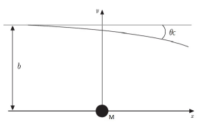
Figure 1: Geometry of the light bending.

Inserting these quantities into Eq. (8), we obtain

$$\Delta p_{2}=\frac{\kappa}{2}p^{1}\int_{-\infty}^{\infty}{\partial_{y}[h_{00}+h_{11}]dx^{1}},$$ (9)

which can be written as

$$\Delta p_{2}=\frac{\kappa}{2}p^{1}\int_{-\infty}^{\infty}{\Big{[}\Big{(}\frac{d}{dr}(h_{00}+h_{11})\Big{)}\frac{\partial r}{\partial y}\Big{]}\Big{|}_{y=b}dx}.$$ (10)

With the result (7), we can rewrite Eq. (10) simply as

$$\Delta p_{2}= \frac{M\kappa^{2}b}{16\pi}p^{1}\int_{-\infty}^{\infty}\Bigg{[}\frac{1}{(x^{2}+b^{2})^{\frac{3}{2}}}$$ (11)

$$-\frac{1+m_{2}(x^{2}+b^{2})^{\frac{1}{2}}}{(x^{2}+b^{2})^{\frac{3}{2}}}e^{-m_{2}(x^{2}+b^{2})^{\frac{1}{2}}}\Bigg{]}dx.$$

Therefore, the classical deflection angle, i.e., $\theta_{\mathrm{C}}\equiv\Big{|}\frac{\Delta p_{y}}{p_{x}}\Big{|}=\Big{|}\frac{-\Delta p_{2}}{p^{1}}\Big{|}$, can be computed through the expression

$$\theta_{\mathrm{C}}=\theta_{\mathrm{E}}-\frac{M\kappa^{2}b}{16\pi}\int_{-\infty}^{\infty}\frac{1+m_{2}(x^{2}+b^{2})^{\frac{1}{2}}}{(x^{2}+b^{2})^{\frac{3}{2}}}e^{-m_{2}(x^{2}+b^{2})^{\frac{1}{2}}}dx,$$

where $\theta_{\mathrm{E}}$ is Einstein’s deflection angle.

At this point, some comments are in order.

1. It is trivial to see from the above result that $\theta_{\mathrm{C}}\rightarrow\theta_{\mathrm{E}}$ as $m_{2}\rightarrow\infty$ ($|\beta|\rightarrow 0$). In other words, in this limit we recover Einstein’s prediction for the light bending. That is the reason why the integration constant related to the mentioned equation is zero. In addition, the limit for $m_{2}\rightarrow 0$ ($|\beta|\rightarrow\infty$) clearly shows the absence of deflection. Both results are physically consistent.

2. The scalar excitation of mass $m_{0}$ does not contribute at all to the light bending. Why is this so? Because the metric concerning linearized $R+R^{2}$ gravity — the theory obtained by linearizing the field equations related to the Lagrangian ${\cal L}=\sqrt{-g}[\frac{2}{\kappa^{2}}R+\frac{\alpha}{2}R^{2}-{\cal L}_{\mathrm{M}}]$ — is conformally related to linearized GR. Indeed, denoting the solution to the linearized $R+R^{2}$ gravity by $g^{(R+R^{2})}_{\mu\nu}$, we promptly obtain $g^{(R+R^{2})}_{\mu\nu}\equiv\eta_{\mu\nu}+\kappa g^{(R+R^{2})}_{\mu\nu}=(1-\kappa\phi)g^{(E)}_{\mu\nu},$ where, of course, terms of order $\kappa^{2}$ were neglected.

3. A quick glance at the equation at hand shows that the dependence of $\theta_{\mathrm{C}}$ on $|\beta|$ is dominated by the exponential term, which suggests that the transition from the Einsteinian limit to the no-deflection scenario might be localized in a well-defined interval. Outside this domain, $\theta_{\mathrm{C}}$ is practically constant. Thence, we come to the conclusion that $0\leq\theta_{\mathrm{C}}\leq\theta_{\mathrm{E}}$.

Numerical integration allows the evaluation of the deflection angle for different values of $|\beta|$. The result for a light ray just grazing the Sun is depicted in Fig. 2. We point out that the transition interval occurs for $10^{84}\lesssim|\beta|\lesssim 10^{88}$. Therefore, in order not to conflict with the prediction of GR for the solar gravitational deflection which, incidentally, has been exhaustively tested experimentally with great success, $|\beta|<10^{84}$.

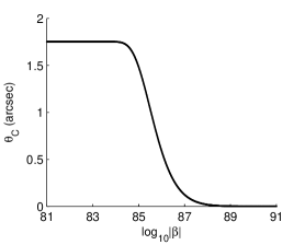
Figure 2: Deflection angle $\theta_{\mathrm{C}}$ as a function of ${\mathrm{log}}_{10}|\beta|$ for light rays just grazing the Sun in classical HDG.

III Gravitational deflection in tree-level hdg

Semiclassical gravity is based on the following type of approximation scheme: the metric is considered as a classical field, predetermined by the gravitational field equations which in our case are those of HDG; besides, the energy content of some particles and/or fields are often neglected. In addition, the spacetime, which is nothing but a fixed background, is determined, uniquely, for example, by a huge, static, point mass $M$. Incidentally, the mass $M$ is huge in comparison to the energy of the other particles and/or fields that either exert a tiny influence on the space time or do not affect it at all. And more, the classical gravitational field interacts with particles that are quantum in nature. As is well known, the results found via a semiclassical gravity theory are more comprehensive than those obtained from the corresponding classical one. In fact, at the classical level we deal with structureless particles, while at the tree level we are involved with quantum particles. Of course, in the classical limit the former results reduce to the latter. As far as GR is concerned, interesting examples related to this subject can be found, for example, in 26 ; 27 ; 28 ; 29 ; 30 .

Let us then analyze the gravitational deflection of a photon within the context of tree-level HDG. Consider, in this vein, the scattering of this photon by the external gravity field (7). The Feynman amplitude for this process is given by (See Fig. 3)

Figure 3: Photon scattering by an external gravitational field. Here $|{\bf{p}}|=|{\bf{p^{\prime}}}|$.

$${\cal{M}}_{rr^{\prime}}= \frac{1}{2}\kappa h^{\lambda\rho}_{\mathrm{ext}}({\bf{k}})\Bigg{[}-\eta_{\mu\nu}\eta_{\lambda\rho}pp^{\prime}+\eta_{\lambda\rho}p^{\prime}_{\mu}p_{\nu}+2\Big{(}\eta_{\mu\nu}p_{\lambda}p^{\prime}_{\rho}$$

$$-\eta_{\nu\rho}p_{\lambda}p^{\prime}_{\mu}-\eta_{\mu\lambda}p_{\nu}p^{\prime}_{\rho}+\eta_{\mu\lambda}\eta_{\nu\rho}pp^{\prime}\Big{)}\Bigg{]}\epsilon^{\mu}_{r}({\bf{p}})\epsilon^{\nu}_{r^{\prime}}({\bf{p^{\prime}}}),$$

where $\epsilon^{\mu}_{r}({\bf{p}})$ and $\epsilon^{\nu}_{r^{\prime}}({\bf{p^{\prime}}})$ are the polarization vectors for the initial and final photons, respectively, which satisfy the completeness relation

$$\sum_{r=1}^{2}\epsilon^{\mu}_{r}({\bf{p}})\epsilon^{\nu}_{r}({\bf{p}})=-\eta^{\mu\nu}-\frac{p^{\mu}p^{\nu}}{(pn)^{2}}+\frac{p^{\mu}n^{\nu}+p^{\nu}n^{\mu}}{pn},$$ (12)

where $n^{2}=1$. Here $h^{\lambda\rho}_{\mathrm{ext}}({\bf{k}})$ is the momentum space gravitational field, namely,

$$h^{\lambda\rho}_{\mathrm{ext}}({\bf{k}})=\int{d^{3}{\bf{r}}e^{-i{\bf{k}}\cdot{\bf{r}}}h^{\lambda\rho}_{\mathrm{ext}}({\bf{r}})}.$$ (13)

Thence,

$$h^{\lambda\rho}_{\mathrm{ext}}({\bf{k}})=h^{{\mathrm{(E)}}\lambda\rho}_{\mathrm{ext}}({\bf{k}})+h^{{\mathrm{(R^{2}_{\mu\nu})}}\lambda\rho}_{\mathrm{ext}}({\bf{k}})+h^{{\mathrm{(R^{2})}}\lambda\rho}_{\mathrm{ext}}({\bf{k}}),$$ (14)

with

$$h^{{\mathrm{(E)}}\mu\nu}_{\mathrm{ext}}({\bf{k}})=\frac{\kappa M}{4{\bf{k}}^{2}}\eta^{\mu\nu}-\frac{\kappa M}{2}\frac{\eta^{\mu 0}\eta^{\nu 0}}{\bf{\bf{k}}^{2}},$$

$$h^{{\mathrm{(R^{2}_{\alpha\beta})}}\mu\nu}_{\mathrm{ext}}({\bf{k}})=-\frac{\kappa M}{6}\frac{\eta^{\mu\nu}}{{\bf{k}}^{2}+m^{2}_{2}}+\frac{\kappa M}{2}\frac{\eta^{\mu 0}\eta^{\nu 0}}{{\bf{k}}^{2}+m^{2}_{2}},$$

$$h^{{\mathrm{(R^{2})}}\mu\nu}_{\mathrm{ext}}({\bf{k}})=-\frac{\kappa M}{12}\frac{\eta^{\mu\nu}}{{\bf{k}}^{2}+m^{2}_{0}}.$$

The unpolarized cross-section can then be written as

$$\frac{d\sigma}{d\Omega} =\frac{1}{(4\pi)^{2}}\frac{1}{2}\sum_{r}\sum_{r^{\prime}}{\cal{M}}^{2}_{rr^{\prime}}$$

$$=\frac{1}{(4\pi)^{2}}\frac{\kappa^{4}M^{2}E^{4}(1+\cos{\theta})^{2}}{16}\Bigg{[}-\frac{1}{{\bf{k}}^{2}}+\frac{1}{{\bf{k}}^{2}+m^{2}_{2}}\Bigg{]}^{2},$$

where $E$ is the energy of the incident photon and $\theta$ is the scattering angle.

For small angles the preceding equations reduces to

$$\frac{d\sigma}{d\Omega}=16G^{2}M^{2}\Big{[}-\frac{1}{\theta^{2}}+\frac{1}{\theta^{2}+\frac{m^{2}_{2}}{E^{2}}}\Big{]}^{2}.$$ (15)

This result signals an energy-dependent scattering.

It is easy to see from (15) that

$$\frac{d\sigma}{d\Omega}\rightarrow 0,\;\;{\mathrm{if}}\;\frac{m_{2}}{E}\rightarrow 0,$$

$$\frac{d\sigma}{d\Omega}\rightarrow\Big{(}\frac{4GM}{\theta^{2}}\Big{)}^{2},\;\;{\mathrm{if}}\;\frac{m_{2}}{E}\rightarrow\infty;$$

in other words, if ${\frac{m_{2}}{E}}\rightarrow 0$, there is no scattering, whereas if $\frac{m_{2}}{E}\rightarrow\infty$, we recover Einstein’s standard cross-section, as expected.

Now, in order to arrive at a classical particle trajectory from (15), we compare the classical and the tree-level cross-section formulas 31 ; 32

$$\frac{d\sigma}{d\Omega}=16G^{2}M^{2}\Bigg{[}-\frac{1}{\theta^{2}}+\frac{E^{2}}{E^{2}\theta^{2}+m^{2}_{2}}\Bigg{]}^{2}=-\frac{rdr}{\theta d\theta}.$$ (16)

Performing the integration we promptly find that for a photon just grazing the Sun the above equation gives the following result

$$\frac{1}{\theta^{2}_{\mathrm{E}}}=\frac{1}{\theta^{2}}+\frac{1}{\lambda^{2}+\theta^{2}}+\frac{2}{\lambda^{2}}\ln{\frac{\theta^{2}}{\lambda^{2}+\theta^{2}}},$$ (17)

with $\lambda^{2}\equiv\frac{m^{2}_{2}}{E^{2}}$. We call attention to the fact that the integration constant related to the this equation was temporarily omitted for the sake of a cautious and meticulous analysis of the behavior of the $\theta$-dependent function we shall perform in the following; of course, it will be restored in due course. To do the aforementioned investigation in a consistent way, we define beforehand a function $\gamma=\gamma\Big{(}\frac{m^{2}_{2}}{E^{2}}\Big{)}>0$ so that the $\theta$ angle can be written as

$$\theta=\gamma\frac{m_{2}}{E}.$$ (18)

As a result, Eq. (17) can be rewritten as

$$\frac{\lambda^{2}}{\theta^{2}_{\mathrm{E}}}=\frac{1}{\gamma^{2}}+\frac{1}{1+\gamma^{2}}+2\ln{\Big{(}\frac{\gamma^{2}}{1+\gamma^{2}}\Big{)}}\equiv f(\gamma),$$ (19)

or

$$\frac{\theta^{2}}{\theta^{2}_{\mathrm{E}}}=\gamma^{2}f(\gamma).$$ (20)

We remark that since $f$ is a monotonically decreasing function of $\gamma$ having as image the interval $(0,+\infty)$, it can be shown that is always possible to find a solution to (17) in the form (18). In addition, $\gamma$ is a decreasing function, implying that the limit $\lambda\rightarrow 0$ corresponds, for instance, to let $\gamma\rightarrow\infty$ in Eq. (20).

We are now ready to analyze the behavior of $\theta$ at different situations. It is straightforward to see that for a fixed energy $E$, $\theta\rightarrow\theta_{\mathrm{E}}$ as $|\beta|\rightarrow 0$ and $\theta\rightarrow 0$ as $|\beta|\rightarrow\infty$. The former regime recovers Einstein’s one, as desirable, while the latter shows that for a sufficient large $|\beta|$ no deflection occurs. We also point out that $0\leq\theta\leq\theta_{\mathrm{E}}$ since $\gamma^{2}f(\gamma)\leq 1$.

The repulsive contribution to the bending, which arrives from the $R^{2}_{\mu\nu}$-sector, is energy dependent as it is evident from (17). Inasmuch as $|\beta|$ is thought to be a (universal) constant, it is worthwhile to analyze the behavior of the scattering angle for a fixed $|\beta|$ and different values of $E$. It is obvious that in this scenario $\theta\rightarrow\theta_{\mathrm{E}}$ in the low energy (classical) limit, and $\theta\rightarrow 0$ for sufficiently energetic photons, suggesting that the more energetic a photon is, the less it will deviate. Let us then show that this is indeed the case by finding the solutions to Eq. (17) for visible light. In Fig. 4 it is shown how $\theta$ behaves for different values of $|\beta|$. A quick glance at this graphic allows us to conclude that for a fixed $E$, the scattering angle for visible light is approximately constant for almost all values of $|\beta|$, making a transition from $\theta\approx\theta_{\mathrm{E}}$ to $\theta\approx 0$ in a well defined interval of width $\Delta|\beta|\approx 10^{10}$.

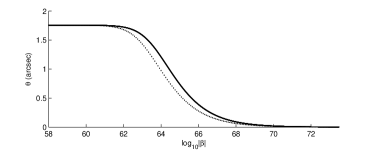
Figure 4: $\theta_{\mathrm{red}}$ (continuum line) and $\theta_{\mathrm{violet}}$ (dotted line) for photons passing by the Sun as a function of $\log_{10}{|\beta|}$ in semiclassical HDG.

Accordingly, in the framework of tree-level HDG the visible spectrum, whose wavelength ranges from 4000 to 7000 (Å), would spread over an angle $|\Delta\theta|$, where $|\Delta\theta|\equiv|\theta_{\mathrm{violet}}-\theta_{\mathrm{red}}|$. Let us then evaluate $|\Delta\theta|$ for different values of $|\beta|$ using Eq. (17). The results are shown in Fig. (5).

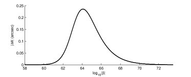
Figure 5: $|\Delta\theta|$ as a function of $\log_{10}{|\beta|}$ for photons passing by the Sun’s limb in the context of tree-level HDG.

A cursory inspection of this graph allows us to conclude that for $61\lesssim\log_{10}{|\beta|}\lesssim 71$ the spread of the visible spectrum would in principle be observable. Actually, we ought to expect a tiny value for $|\Delta\theta|$ at the Sun’s limb in order not to conflict with well established results of experimental general relativity. Consequently, if $|\beta|<10^{61}$, the visible spectrum spread would be practically imperceptible and the deviation angle would be very close to the Einstein one. Accordingly, we come to the conclusion that in order to agree with the currently measured values for visible light, $|\beta|<10^{61}$. We point out that this bound was estimated by noting that the gravitational rainbow predicted by tree-level HDG is incompatible with today measurements. Of course, the mentioned limit would be modified if we have made use of photons with wavelength outside the domain of the visible light.

IV Smooth transition from the semiclassical context to the classical one

The most striking difference between the classical and semiclassical approaches is, perhaps, the fact that the repulsive interaction owed to the $R^{2}_{\mu\nu}$-sector depends on the photon energy that interacts with the gravitational field. Since in the classical realm the gravitational field acts on structureless particles, gravity scatters light of all wavelengths in the same way; nonetheless, in the tree-level scenario more energetic photons are more repelled and, as consequence, less deflected.

Now, a point that deserves a careful attention is the subtle divergence between these scenarios at low energy: the classical limit of the semiclassical theory does not match that of classical HDG. In fact, in the classical model, whatever the energy of the light ray is, no scattering will occur if $|\beta|>10^{89}$. On the other hand, the analysis at the tree-level does not impose any upper bound at all on the interval of the $|\beta|$ transition; consequently, it is always possible to find a small $E$ so that $\theta$ is arbitrarily close to $\theta_{\mathrm{E}}$, even if $|\beta|>10^{89}$. A way out of this difficulty, would be to add a non trivial integration constant to Eq. (17) which, as a result, assumes the form

$$\frac{1}{\theta^{2}_{\mathrm{E}}}=\frac{1}{\theta^{2}}+\frac{1}{\lambda^{2}+\theta^{2}}+\frac{2}{\lambda^{2}}\ln{\frac{\theta^{2}}{\lambda^{2}+\theta^{2}}}-\Omega,$$ (21)

Indeed, choosing $\Omega$ as a function only of $|\beta|$, it is possible to make it to give a negligible contribution in the range of energies such that the transition occurs for $|\beta|\lesssim 10^{85}$, and to be relevant for the photons which make its transition above this interval.

Let us then compare the deflection angles computed in both frameworks, i.e., $\theta$ and $\theta_{\mathrm{C}}$, requiring furthermore that $\theta\rightarrow\theta_{\mathrm{C}}$ if $E\rightarrow 0$. Using the limit calculated in Sec. 3, Eq. (21) reduces to

$$\frac{1}{\theta^{2}_{\mathrm{E}}}=\frac{1}{\theta^{2}}-\Omega,$$ (22)

whose solution is

$$\theta=\theta_{\mathrm{E}}\Big{(}1+\Omega\theta^{2}_{\mathrm{E}}\Big{)}^{-\frac{1}{2}}.$$ (23)

Now, imposing that $\theta=\theta_{C}$, we promptly obtain

$$\Omega=\frac{1}{\theta^{2}_{\mathrm{C}}}-\frac{1}{\theta^{2}_{\mathrm{E}}}.$$ (24)

Our next step is to check whether the Einsteinian limit ($|\beta|\rightarrow 0$) is indeed consistent. In Sec. 2 we got that $\theta_{\mathrm{C}}\rightarrow\theta_{\mathrm{E}}$ if $|\beta|\rightarrow 0$, and, as a result, $\Omega\rightarrow 0$. Moreover, it is easy to see that $\Omega\gg\theta^{-2}_{\mathrm{E}}$ if ${|\beta|\gtrsim 10^{88}}$. Therefore, the limit $|\beta|\rightarrow 0$ remains unchanged, and Einstein solar deflection angle is recovered, as it should. We point out that for $|\beta|<10^{85}$ the integration constant $\Omega$ can be simply neglected. For larger values of $|\beta|$, nevertheless, $\Omega$ increases too quickly forcing $\theta\rightarrow 0$ even for low energy photons. Besides, the classical results are recovered in the classical limit. In Figs. 6 and 7 we display some values of $\Omega$ for different $|\beta|$s.

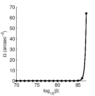
Figure 6: $\Omega$ as a function of $|\beta|$. It is worth noting that $\Omega$ is roughly zero for $|\beta|<10^{85}$, where it starts the approximately double exponential growth depicted in Fig. 7.

Two comments fit here.

1. We have shown in Sec. 3 that for visible light the transition from $\theta_{\mathrm{E}}$ to 0 in the absence of the integration constant took place for $|\beta|\in(10^{61},10^{71})$. Making use of these values an upper bound on $|\beta|$ was estimated. We remark that this result remains unchanged since within the mentioned domain, as we have proved, $\Omega$ can be taken to be equal zero.

2. In order to allow the deflection angle computed at the tree level to agree in the classical limit with the result found directly via the classical approach, we have to appeal to the integration constant $\Omega$ (See (22)). On the other hand, for $|\beta|<10^{85}$ this constant is tiny, implying that it can be left out of any computation if we take the current experimental accuracy into account. Now, since $|\beta|<10^{84}$ is the upper bound on $|\beta|$ found classically, and $|\beta|<10^{61}$ is that arising from the tree-level computations, we come to the conclusion that the constant $\Omega$ can be simply neglected.

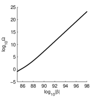
Figure 7: $\Omega$ (in arcs^-2) for some values of $|\beta|$. Here the $\Omega$-axis scale is also logarithmic in order to show its quick increase for $|\beta|>10^{85}$.

V Final remarks

We have shown that the photon propagation in the framework of tree-level HDG is dispersive. From the analysis of the energy-dependent contribution coming from the photons passing by the Sun, it was possible to estimate an upper bound on $|\beta|$, namely, $|\beta|<10^{61}$. Let us then compare this upper limit with that available in the literature. Using the interesting measures of Long 33 , Stelle 34 found that $m_{2}\approx 1\times 10^{-4}cm^{-1}$. From this value Donoghue 35 estimated that $|\beta|\leq 10^{74}$. Therefore, our bound lowered the accepted limit on $|\beta|$ by thirteen orders of magnitude.

We call attention to the fact that the measurements made in the radio band, despite its precision and accuracy, do not improve the limit on $|\beta|$ we have found. In fact, since less energetic photons undergo a greater bending, the transition interval from $\theta=\theta_{\mathrm{E}}$ to $\theta=0$ occurs for the measured radio waves about 10 orders of magnitude above the visible waves. However, if gravitational deflection measurements in the X-ray or ultraviolet bands were available, we could certainly improve the limit on $|\beta|$. Unfortunately, it is a very hard task to separate the signs present in these wavelengths from those emitted by the Sun. Accordingly, we come to the conclusion that the bound we have obtained is the best limit one can found using the gravitational deflection measurements available nowadays.

To conclude, we mention that we have estimated a bound on the constant of the $R^{2}$-sector of HDG using the accurate experimental results we have at our disposal today concerning the gravitational red shift of the spectral lines. This limit will be published elsewhere 36 . Interestingly enough, the cited classical text of GR was the first conceived by Einstein to verify his theory but the last to have reliable experimental results.

- (1) D. Lebach et al., Phys. Rev. Lett. 75, 1439 (1995).
- (2) E. Fomalont, S. Kopeikin, G. Lanyi, and J. Benson, Astrophys. J. 699, 1395 (2009).
- (3) H. Weyl, Space-Time Matter (Dover, 1952).
- (4) A. Eddington, The Mathematical Theory of Relativity, 2nd. ed. (Cambridge University Press, 1924).
- (5) P. Havas, Gen. Relativ. Gravit. 8, 631 (1977).
- (6) K. Stelle, Phys. Rev. D 16, 953 (1977).
- (7) I. Antoniadis and E. Tomboulis, Phys. Rev. D 33, 2756 (1986).
- (8) D. Johnston, Nucl. Phys. B 297, 721 (1988).
- (9) M. Ostrogradski, Mem. Ac. St. Petersburg 6 (4), 385 (1850).
- (10) T. Nakamura and S. Hamamoto, Prog. Theor. Phys. 95, 469 (1996).
- (11) R. Woodard, Lect. Notes Phys. 720, 403 (2007).
- (12) M. Plyushchay, Mod. Phys. Lett. A 4, 837 (1989).
- (13) E. Bergshoeff, O. Holm, and P. Townsend, Phys. Rev. Lett. 102, 201301 (2009).
- (14) S. Deser, Phys. Rev. Lett. 103, 101302 (2009).
- (15) A. Accioly, J. Helayël-Neto, J. Morais, E. Scatena, and R. Turcati, Phys. Rev. D 83, 104005 (2011).
- (16) A. Accioly, J. Helayël-Neto, E. Scatena, J. Morais, R. Turcati and B. Pereira-Dias Class. Quantum Grav. 28, 225008 (2011).
- (17) A. Accioly, A. Azeredo, and H. Mukai, J. Math. Phys. 43, 473 (2002).
- (18) T. Soritiou and V. Faraoni, Rev. Mod. Phys. 82, 451 (2010).
- (19) I. Shapiro, A. Pelinson and F. Salles, Mod. Phys. Lett. A 29, 1430034 (2014).
- (20) F. Salles and I. Shapiro, Phys. Rev. D 89, 084054 (2014).
- (21) A. Accioly, J. Helayël-Neto, F. E. Barone, and Wallace Herdy, Class. Quantum Grav. 32, 035021 (2015).
- (22) M. Veltman, in Methods in Field Theory, eds. R. Balian and J. Zinn-Justin (North Holland/World Scientific, 1981).
- (23) P. Teyssandier Class. Quantum Grav. 6, 219 (1989).
- (24) A. Accioly, A. Azeredo, H. Mukai, and E. de Rey-Neto, Prog. Theor. Phys. 104, 103 (2000).
- (25) A. Accioly, J. Helayël-Neto, F. E. Barone, F. A. Barone, and P. Gaete, Phys. Rev. D 90, 105029 (2014).
- (26) R. Paszko and A. Accioly, Class. Quantum Grav. 27, 145012 (2010).
- (27) A. Accioly and R. Paszko, Int. J. Mod. Phys. D 18, 2107 (2009).
- (28) A. Accioly and R. Paszko, Adv. Stud. Theor. Phys. 3, 65 (2009).
- (29) A. Accioly and R. Paszko, Phys. Rev. D 78, 064002 (2008).
- (30) A. Accioly, R. Aldrovandi, and R. Paszko, Int. J. Mod. Phys. D 15, 2249 (2006).
- (31) R. Delbourgo and P. Phocas-Cosmetatos, Phys. Lett. B 41, 533 (1972).
- (32) F. Berends and R. Gastmans, Ann. Phys. (N. Y.) 98, 225 (1976).
- (33) D. Long, Nature 260, 417 (1976).
- (34) K. Stelle, Gen. Relativ. Gravit. 9, 353 (1978).
- (35) J. Donoghue, Phys. Rev. Lett. 72, 2996 (1994).
- (36) B. Giacchini, Upper bounds on the free parameters of higher-derivative gravity (to be published).