Privacy for the Protected (Only)

Abstract

Motivated by tensions between data privacy for individual citizens, and societal priorities such as counterterrorism and the containment of infectious disease, we introduce a computational model that distinguishes between parties for whom privacy is explicitly protected, and those for whom it is not (the targeted subpopulation). The goal is the development of algorithms that can effectively identify and take action upon members of the targeted subpopulation in a way that minimally compromises the privacy of the protected, while simultaneously limiting the expense of distinguishing members of the two groups via costly mechanisms such as surveillance, background checks, or medical testing. Within this framework, we provide provably privacy-preserving algorithms for targeted search in social networks. These algorithms are natural variants of common graph search methods, and ensure privacy for the protected by the careful injection of noise in the prioritization of potential targets. We validate the utility of our algorithms with extensive computational experiments on two large-scale social network datasets.

1 Introduction

The tension between useful or essential gathering and analysis of data about citizens, and the privacy rights of those citizens, is at an historical peak. Perhaps the most striking and controversial recent example is the revelation that U.S. intelligence agencies systemically engage in “bulk collection” of civilian “metadata” detailing telephonic and other types of communication and activities, with the alleged purpose of monitoring and thwarting terrorist activity [9]. Other compelling examples abound, including in medicine (patient privacy vs. preventing epidemics), marketing (consumer privacy vs. targeted advertising), and many other domains.

Debates about (and models for) data privacy often have an “all or nothing” flavor: privacy guarantees are either provided to every member of a population, or else privacy is deemed to be a failure. This dichotomy is only appropriate if all members of the population have an equal right to, or demand for, privacy. Few would argue that actual terrorists should have such rights, which leads to difficult questions about the balance between protecting the rights of ordinary citizens, and using all available means to prevent terrorism. A major question is whether and when the former should be sacrificed in service of the latter. Similarly, in the medical domain, epidemics (such as the recent international outbreak of Ebola [14]) have raised serious debate about the clear public interest in controlling contagion versus the privacy rights of the infected and those that care for them.

The model and results in this paper represent a step towards explicit acknowledgments of such trade-offs, and algorithmic methods for their management. The scenarios sketched above can be broadly modeled by a population divided into two types. There is a protected subpopulation that enjoys (either by law, policy, or choice) certain privacy guarantees. For instance, in the examples above, these protected individuals might be non-terrorists, or uninfected citizens (and perhaps informants and health care professionals). They are to be contrasted with the “unprotected” or targeted subpopulation, which does not share those privacy assurances. A key assumption of the model we will introduce is that the protected or targeted status of individual subjects is not known, but can be discovered by (possibly costly) measures, such as surveillance or background investigations (in the case of terrorism) or medical tests (in the case of disease). Our overarching goal is to allow parties such as intelligence or medical agencies to identify and take appropriate actions on the targeted subpopulation, while also providing privacy assurances for the protected individuals who are not the specific targets of such efforts — all while limiting the cost and extent of the background investigations needed.

As a concrete example of the issues we are concerned with, consider the problem of using social network data (for example, telephone calls, emails and text messages between individuals) to search for candidate terrorists. One natural and broad approach would be to employ common graph search methods: beginning from known terrorist “seed” vertices in the network, neighboring vertices are investigated, in an attempt to “grow” the known subnetwork of targets. A major concern is that such search methods will inevitably encounter protected citizens, and that even taking action against only discovered targeted individuals may compromise the privacy of the protected.

In order to rigorously study the trade-offs between privacy and societal interests discussed above, our work introduces a formal model for privacy of network data that provides provable assurances only to the protected subpopulation, and gives algorithms that allow effective investigation of the targeted population. These algorithms are deliberately “noisy” and are privacy-preserving versions of the widely used graph search methods mentioned above, and as such represent only mild (but important) departures from commonly used approaches. At the highest level, one can think of our algorithms as outputting a list of targeted individuals discovered in the network for which any subsequent action (e.g. publication in a most-wanted list, further surveillance or arrest in the case of terrorism, or medical treatment or quarantine in the case of epidemics) will not compromise the privacy of the protected.

The key elements of our model include the following:

1. Network data collected over a population of individuals and consisting of pairwise contacts (physical, social, electronic, financial, etc.). The contacts or links of each individual comprise the private data they desire to protect. We assume a third party (such as an intelligence agency or medical organization) has direct access to this network data, and would like to discover and act upon targeted individuals.

2. For each individual, an immutable status bit that determines their membership status in the targeted subpopulation (such as terrorism or infection). These status bits can be discovered by the third party, but only at some nontrivial cost (such as further surveillance or medical testing), and thus there is a budget limiting the number of status bits that an algorithm can reveal. One might assume or hope that in practice, this budget is sufficient to investigate a number of individuals that is of the order of the targeted subpopulation size, but considerably less than that needed to investigate every member of the general population.

3. A mathematically rigorous notion of individual data privacy (based on the widely studied differential privacy [5]) that provides guarantees of privacy for the network data of only the protected individuals, while allowing the discovery of targeted individuals. Informally, this notion guarantees that compared to a counterfactual world in which any protected individual arbitrarily changed any part of their data, or even removed themselves entirely from the computation, their risk (measured with respect to the probability of arbitrary events) has not substantially increased.

Our main results are:

1. The introduction of a broad class of graph search algorithms designed to find and identify targeted individuals. This class of algorithms is based on a general notion of a statistic of proximity — a network-based measure of how “close” a given individual $v$ is to a certain set of individuals $S$. For instance, one such closeness measure is the number of short paths in the network from $v$ to members of $S$. Our (necessarily randomized) algorithms add noise to such statistics in order to prioritize which status bits to query (and thus how to spend the budget).

2. A theoretical result providing a quantitative privacy guarantee for this class of algorithms, where the level of privacy depends on a measure of the sensitivity of the statistic of proximity to small changes in the network.

3. Extensive computational experiments in which we demonstrate the effectiveness of our privacy-preserving algorithms on real social network data. These experiments demonstrate that in addition to the privacy guarantees, our algorithms are also useful, in the sense that they find almost as many members of the targeted subpopulation as their non-private counterparts. The experiments allow us to quantify the loss in effectiveness incurred by the gain in privacy.

We note that although our class of network search algorithms is relatively broad, it necessarily excludes some natural and commonly used algorithms. This is by design, since some algorithms are clearly in conflict with the kind of privacy we wish to protect for protected individuals.

To our knowledge, our formal framework is the first to introduce explicit protected and targeted subpopulations with qualitatively differing privacy rights, and our algorithms the first to provide mathematically rigorous privacy guarantees for the protected while still allowing effective discovery of the targeted. More generally, we believe our work is a first step towards richer privacy models that acknowledge and manage the tensions between different levels of privacy guarantees to different subgroups.

2 Preliminaries

Consider a social network in which the individuals are partitioned into a targeted subpopulation $\mathcal{T}$ and a protected subpopulation $\mathcal{P}$. Individuals correspond to the vertices $V$ in the network, and the private data of each individual $v$ is the set of edges incident to $v$. Each individual also has an immutable status bit which specifies to which subpopulation the individual belongs. We assume that the value of this bit is not easily observed, but can be discovered through (possibly costly) investigation. Our goal is to develop search algorithms to identify members of the targeted subpopulation, while preserving the privacy of the edge set of the protected population.

Any practical algorithm must operate under an investigation budget, which limits the number of status bits that are examined. Our goal is a total number of status bit examinations that is on the order of the size of the targeted subpopulation $\mathcal{T}$, which may be much smaller than the size of the protected population $\mathcal{P}$. This is the source of the tension we study — because the budget is limited, it is necessary to exploit the private edge set to guide our search (i.e. we cannot simply investigate the entire population), but we wish to do so in a way that does not reveal much about the edges incident to any specific individual.

The privacy guarantee we provide is a variant of differential privacy, an algorithmic definition of data privacy. It formalizes the requirement that arbitrary changes to a single individual’s private data should not significantly affect the output distribution of the data analysis procedure, and so guarantees that the analysis leaks little information about the private data of any single individual. We first introduce the definition of differential privacy specialized for the network setting. We treat networks as a collection of vertices representing individuals, each represented as a list of its edges (which form the private data of each vertex). For a network $G$ and a vertex $v$, let $D_{v}(G)$ be the set of edges incident to the vertex $v$ in $G$. Let $\mathcal{G}_{n}$ be the family of all $n$-vertex networks.

Definition 1 (Vertex Differential Privacy [5, 10]).

The networks $G,G^{\prime}$ in $\mathcal{G}_{n}$ are neighboring if one can be obtained from the other by an (arbitrary) rewiring of the edges incident to a single vertex $v$ — i.e. if for some vertex $v$, $D_{u}(G)\setminus\{(u,v)\}=D_{u}(G^{\prime})\setminus\{(u,v)\}$ for all $u\neq v$. An algorithm $\mathcal{A}\colon\mathcal{G}_{n}\rightarrow\mathcal{O}$ satisfies $\varepsilon$-differential privacy if for every event $S\subseteq\mathcal{O}$ and all neighboring networks $G,G^{\prime}\in\mathcal{G}_{n}$,

$$\Pr[\mathcal{A}(G)\in S]\leq e^{\varepsilon}\Pr[\mathcal{A}(G^{\prime})\in S].$$

Differential privacy is an extremely strong guarantee — it has many interpretations (see discussion in e.g. [7]), but most straightforwardly, it promises the following: simultaneously for every individual $i$, and simultaneously for any event $S$ that they might be concerned about, event $S$ is almost no more likely to occur given that individual $i$’s data is used in the computation, compared to if it were replaced by an arbitrarily different entry. Here, “almost no more likely” means that the probability that the bad event $S$ occurs has increased by a multiplicative factor of at most $e^{\varepsilon}$, which we term the risk multiplier. As the privacy parameter $\varepsilon$ approaches $0$, the value of the risk multiplier approaches $1$, meaning that agent $i$’s data has no effect at all on the probability of a bad outcome. The smaller the risk multiplier, the more meaningful the privacy guarantee. It will be easier for us to reason directly about the privacy parameter $\varepsilon$ in our analyses, but semantically it is the risk multiplier $e^{\varepsilon}$ that measures the quality of the privacy guarantee, and it is this quantity that we report in our experiments.

Differential privacy promises the same protections for every individual in a network, which is incompatible with our setting. We want to be able to identify members of the targeted population, and to do so, we want to be able to make arbitrary inferences from their network data. Nevertheless, we want to give strong privacy guarantees to members of the protected subpopulation. This motivates our variant of differential privacy, which redefines the neighboring relation. In contrast to the definition of neighbors given above, we now say that two networks are neighbors if one can be obtained from the other by arbitrarily re-wiring the edges incident to a single member of the protected population. Crucially, networks are not considered to be neighbors if they differ in either:

1. The way in which they partition vertices between the protected and targeted populations $\mathcal{P}$ and $\mathcal{T}$, or

2. In any edges that connect pairs of vertices $u,v\in\mathcal{T}$ that are both members of the targeted population.

What this means is that we are offering no guarantees about what an observer can learn about either the status of an individual (protected vs. targeted), or the set of edges incident to targeted individuals. However, we are still promising that no observer can learn much about the set of edges incident to any member of the protected subpopulation. This naturally leads us to the following definition:

Definition 2 (Protected Differential Privacy).

Two networks $G,G^{\prime}$ in $\mathcal{G}_{n}$ are neighboring if they:

1. Share the same partition into $\mathcal{P}$ and $\mathcal{T}$, and

2. $G$ can be obtained from $G^{\prime}$ by rewiring the set of edges incident to a single vertex $v\in\mathcal{P}$.

An algorithm $\mathcal{A}\colon\mathcal{G}_{n}\rightarrow\mathcal{O}$ satisfies $\varepsilon$-protected differential privacy if for any two neighboring networks $G,G^{\prime}\in\mathcal{G}_{n}$, and for any event $S\subseteq\mathcal{O}$:

$$\Pr[\mathcal{A}(G)\in S]\leq e^{\varepsilon}\Pr[\mathcal{A}(G^{\prime})\in S].$$

Formally, our network analysis algorithms take as input a network and a method by which they may query whether vertices $v$ are members of the protected population $\mathcal{P}$ or not. The class of algorithms we consider are network search algorithms — they aim to identify some subset of the targeted population. Our privacy guarantees are oblivious as to what action is taken on the identified members (for example, in a medical application they might be quarantined, in a security application they might be arrested, etc.), but we assume that whatever action is taken might be observable. Hence, without loss of generality we can abstract away the action taken and simply view the output of the mechanism to be an ordered list of targeted individuals.

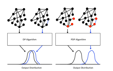
Figure 1: Informal illustration of standard Differential Privacy (DP) versus Protected Differential Privacy (PDP). For algorithms satisfying standard DP (left), the addition of a single edge (dashed blue) can alter the output distribution by only a small amount. PDP is similar, except we introduce a targeted subpopulation (highlighted in red). If the added edge is between two targeted individuals, the output distribution may change arbitrarily, reflecting the fact that the targeted parties may not enjoy privacy protection. The formal definitions are stronger, in that privacy for protected individuals must be preserved even if any number of edges to them is added or deleted.

3 Algorithmic Framework

The key element in our algorithmic framework is the notion of a Statistic of Proximity (SoP), a network-based measure of how close an individual is to another set of individuals in a network. Formally, an SoP is a function $f$ that takes as input a graph $G$, a vertex $v$ and a set of targeted vertices $S\subseteq\mathcal{T}$, and outputs a numeric value $f(G,v,S)$. Examples of such functions include the number of common neighbors between $v$ and the vertices in $S$, and the number of short paths from $v$ to $S$.

Algorithms in our framework rely on the SoP to prioritize which status bits to examine. Since the value of the SoP depends on the protected vertex’s private data, we perturb the values of the SoP by adding noise with scale proportional to its sensitivity, which captures the magnitude by which a single protected vertex can affect the SoP of some targeted vertex. Let $G\sim G^{\prime}$ denote two neighboring networks in $\mathcal{G}$. The sensitivity of the SoP $f$ is defined as:

$$\Delta(f)=\max_{G\sim G^{\prime},t\in\mathcal{T},S\subseteq\mathcal{T}}\left|f(G,t,S)-f(G^{\prime},t,S)\right|.$$

Crucially, note that in this definition — in contrast to what is typically required in standard differential privacy — we are only concerned with the degree to which a protected individual can affect the SoP of a targeted individual.

We next describe the non-private version of our targeted search algorithm $\mbox{{\sf Target}}(k,f)$. For any fixed SoP $f$, Target proceeds in $k$ rounds, each corresponding to the identification of a new connected component in the subgraph induced by $\mathcal{T}$. The algorithm must be started with a “seed vertex” — a pre-identified member of the targeted population. Each round of the algorithm consists of two steps:

1. Statistic-First Search: Given a seed targeted vertex, the algorithm iteratively grows a discovered component of targeted vertices, by examining, in order of their SoP values, the vertices that neighbor the previously discovered targeted vertices. This continues until every neighbor of the discovered members of the targeted population has been examined, and all of them have been found to be members of the protected population. We note that this procedure discovers every member of the targeted population that is part of the same connected component as the seed vertex, in the subgraph induced by only the members of the targeted population.

2. Search for a New Component: Following the completion of statistic-first search, the algorithm must find a new vertex in the targeted population to serve as an initial vertex to begin a new round of statistic-first search. To do this, the algorithm computes the value of the SoP $f$ evaluated on each unexamined vertex, using as the input set $S$ the set of already discovered members of the targeted population. It then sorts all of the vertices in decreasing order of their SoP value, and begins examining them in this order. The first vertex that is found to be a member of the targeted population is used as an initial vertex in the next iteration (taking the place of our seed vertex). We skip this search procedure in the last iteration.

The algorithm outputs discovered targeted individuals as they are found, and so its output can be viewed as being an ordered list of targeted individuals.

The private version of the targeting algorithm $\mbox{{\sf PTarget}}(k,f,\varepsilon)$, is a simple variant of the non-private version. The statistic-first search stage remains unchanged, and only the search for a new component is modified. In the private variant, when the algorithm computes the value of the SoP $f$ on each unexamined vertex, it then perturbs each of these values with noise sampled from the Laplace distribution $\operatorname{Lap}(\triangle(f)/\varepsilon)$ where $\varepsilon$ is a parameter. Finally, it examines the vertices in sorted order of their perturbed SoP values.

We prove the following, deferring details of the proof and the algorithm to the Technical Appendix:

Theorem 1.

Given any $k\geq 1$ and $\varepsilon>0$ and a fixed SoP $f$, the algorithm $\mbox{{\sf PTarget}}(k,f,\varepsilon)$ recovers $k$ connected components of the subgraph induced by the targeted vertices and satisfies $((k-1)\cdot\varepsilon)$-protected differential privacy.

There are two important things to note about this theorem. First, we obtain a privacy guarantee despite the fact that the statistic-first search portion of our algorithm is not randomized — only the search for new components employs randomness. Second, the privacy cost of the algorithm grows only with $k$, the number of disjoint connected components of targeted individuals (disjoint in the subgraph defined on targeted individuals), and not with the total number of individuals examined, or even the total number of targeted individuals identified. Hence, the privacy cost can be very small on graphs in which the targeted individuals lie only in a small number of connected components or “cells”. Both of these features are unusual when compared with typical guarantees that one can obtain under the standard notion of differential privacy.

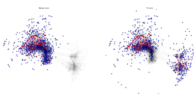
Figure 2: Visual comparison of the non-private algorithm Target (left panel) and the private algorithm PTarget (right panel) on a small portion of the IMDB network (see Experimental Evaluation for more details). For each algorithm, blue indicates protected vertices that have been examined, red indicates targets that have been examined, and gray vertices have not been examined yet. Both algorithms begin with the same seed target vertex, and by directed statistic-first search discover a subnetwork of targeted individuals (central red edges). As a consequence, many protected vertices are discovered and examined as well. Due to the added noise, PTarget explores the network in a more diffuse fashion, which in this case permits it to find an additional subnetwork of targets towards the right side of the network. The primary purpose of the noise, however, is for the privacy of protected vertices.

Because PTarget adds randomness for privacy, it results in examining a different set of vertices as compared to Target. Figure 2 provides a sample visualization of the contrasting behavior of the two algorithms. While theorems comparing the utility of Target and PTarget are possible, they require assumptions ensuring that the chosen SoP is sufficiently “informative”, in the sense of separating the targeted from the protected by a wide enough margin. In particular, one needs to rule out cases in which all unexplored targeted vertices are deemed closer to the current set than all protected vertices, but only by an infinitesimal amount, in which case the noise added by PTarget eradicates all signal. In general such scenarios are unrealistic, so instead of comparing utility theoretically, we now provide an extensive empirical comparison.

4 Experimental Evaluation

In this section we empirically demonstrate the utility of our private algorithm PTarget by comparing its performance to its non-private counterpart Target. We report on computational experiments performed on real social network data drawn from two sources — the paper coauthorship network of DBLP (“Digital Bibliography and Library Project”)[4], and the co-appearance network of film actors of IMDB (“Internet Movie Database”)[11] — whose macroscopic properties are summarized in Table 1.

Table 1: Social network datasets used in the experiments.

Network	Number of vertices	Number of edges	Edge relation
DBLP	956,043	3,738,044	scientific paper co-authorship
IMDB	235,710	4,587,715	movie co-appearance

These data sources provide us with naturally occurring networks, but not a targeted subpopulation. While one could attempt to use communities within each network (e.g. all co-authors within a particular scientific subtopic), our goal was to perform large-scale experiments in which the component structure of targeted vertices (which we shall see is the primary determinant of performance) could be more precisely controlled. We thus used a simple parametric stochastic diffusion process (described in the Technical Appendix) to generate the targeted subpopulation in each network. We then evaluate our private search algorithm PTarget on these networks, and compare its performance to the non-private variant Target. For brevity we shall describe our results only for the IMDB network; results for the DBLP network are quite similar.

In our experiments, we fix a particular SoP: the number of common neighbors between the vertex $v$ and the subset of vertices $S$ representing the already discovered members of the targeted population. This SoP has sensitivity $1$, and so can be used in our algorithm while adding only a small amount of noise. In particular, the private algorithm PTarget adds noise sampled from the Laplace distribution $\operatorname{Lap}(20)$ to the SoP when performing new component search. By Theorem 1, such an instantiation of PTarget guarantees $((k-1)/20)$-protected differential privacy if it finds $k$ targeted components.

The main trade-off we explore is the number of members of the targeted population that are discovered by the algorithms, as a function of the number of status bits that have been investigated. In each of the ensuing plots, the $x$-axis measures the size of the investigation budget consumed so far, while the $y$-axis measures the number of targeted vertices identified for a given budget. In each plot, the parameters of the diffusion model described above were fixed and used to stochastically generate targeted subpopulations of the fixed networks given by our social network data. By varying these parameters, we can investigate performance as a function of the underlying component structure of the targeted subnetwork. As we shall see, in terms of relative performance, there are effectively three different regimes of the diffusion model (i.e. targeted subpopulation) parameter space. In all of them PTarget compares favorably with Target, but to different extents and for different reasons that we now discuss. We also plot the growth of the risk multiplier for PTarget, which remains less than 2 in all three regimes.

On each plot, there is a single blue curve showing the performance of the (deterministic) algorithm Target, and multiple red curves showing the performance across 200 runs of our (randomized) algorithm PTarget.

The first regime (Figure 3) occurs when the largest connected component of the targeted subnetwork is much larger than all the other components. In this regime, if both algorithms begin at a seed vertex inside the largest component, there is effectively no difference in performance, as both algorithms remain inside this component for the duration of their budget and find identical sets of targeted individuals. More generally, if the algorithms begin at a seed outside the largest component, relative performance is a “race” to find this component; the private algorithm lags slightly due to the added noise, but is generally quite competitive.

The second regime (Figure 4) occurs when the component sizes are more evenly distributed, but there remain a few significantly larger components. In this setting both algorithms spend more of their budget outside the targeted subpopulation “searching” for these components. Here the performance of the private algorithm lags more significantly — since both algorithms behave the same when inside of a component, the smaller the components are, the more detrimental the noise is to the private algorithm.

The third regime (Figure 5) occurs when all the targeted components are small, and thus both algorithms suffer accordingly, discovering only a few targeted individuals.

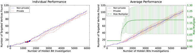
Figure 3: Performance for the cases in which there is a dominant component in the targeted subpopulation. In the left panel, we show the number of targeted vertices found as a function of the budget used for both the (deterministic) non-private algorithm Target (blue), and for several representative runs of the randomized private algorithm PTarget (red). Circles indicate points at which an algorithm has first discovered a new targeted component. In the right panel, we show average performance over 200 trials for the private algorithm with 1-standard deviation error bars. We also show the private algorithm risk multiplier with error bars. In this regime, after a brief initial flurry of small component discovery, both algorithms find the dominant component, so the private performance closely tracks non-private, and the private risk multiplier quickly levels off at around only 1.17.

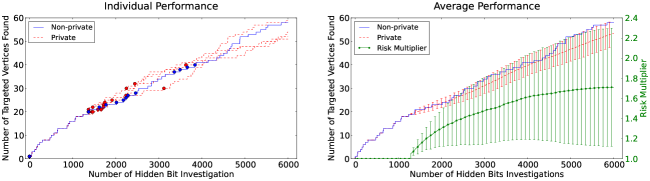
Figure 4: Same format as in Figure 3, but now in a case where the component sizes are more evenly distributed, but still relatively large. The performance of both algorithms is hampered by longer time spent investigating non-targeted vertices (note the scale of the $y$ axis compared to Figure 3). Targeted component discovery is now more diffuse. The private algorithm remains competitive but lags slightly, and as per Theorem 1 the risk multiplier grows as more targeted components are discovered (but remains modest).

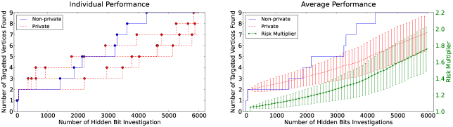
Figure 5: A case with a highly fragmented targeted subpopulation. Both algorithms now spend most of their budget investigating non-targeted vertices and suffer accordingly.

Technical Appendix

Appendix A Model & Preliminaries

We study graph search algorithms which operate on graphs $G=(V,E)$ defined over a vertex set $V$ and edge set $E\subseteq V\times V$. The vertex set $V$ partitioned into two fixed subsets $V=\mathcal{T}\cup\mathcal{P}$, where $\mathcal{T}$ represents the targeted subpopulation, and $\mathcal{P}$ represents the protected subpopulation. The algorithms we consider are initially given a single seed vertex $s\in\mathcal{T}$ (or several such vertices), and the goal of the algorithm will be to find as many other members of the targeted subpopulation $\mathcal{T}$ as possible.

The algorithm cannot directly observe which subpopulation a particular vertex $v\in V$ belongs to since otherwise the problem is trivial, but it has the ability to make a query on a vertex $v\in V$ to determine its subpopulation membership. We model this ability formally by giving the algorithm access to an identity oracle $\mathcal{I}\colon V\to\{0,1\}$, defined such that $\mathcal{I}(v)=1$ if and only if $v\in\mathcal{T}$. A call to this oracle is the abstraction we use to represent the possibly costly operation (instantiated in our example applications by e.g. surveillance, or medical tests) which determines whether a particular member of the population is protected or not. Because we view these operations as expensive, we want our algorithm to operate by making as few calls to this oracle as possible. Hence, the algorithm must use the network data represented by the graph $G$ to guide its search for which vertices to query. This creates a source of privacy tension since the edges in this network are what we view as private information.

Thus our goal is to give algorithms which discover members of the targeted population using the edges in the network to guide their search. We wish to protect the privacy of the protected individuals: we do not want the outcome of the search to reveal too much about the edge set incident to any protected individual. However, we want to exploit the edges incident to targeted individuals in ways that will not necessarily be privacy preserving. The notion of privacy that we employ is a variant of differential privacy. To formally define differential privacy, we consider databases which are multisets of elements from an abstract domain $\mathcal{X}$, representing the set of all possible data records. (In our case, the data domain $\mathcal{X}$ can be identified with subsets of the vertex set $V$ – it represents the set of all possible neighbors that a vertex might be adjacent to in the network).

Definition 3 (Differential Privacy [5]).

Two databases $D,D^{\prime}\subset\mathcal{X}$ are neighbors if they differ in at most one data record: that is, if there exists an index $i$ such that for all indices $j\neq i$, $D_{j}=D^{\prime}_{j}$. An algorithm $\mathcal{A}\colon\mathcal{X}^{n}\rightarrow\mathcal{R}$ satisfies $(\varepsilon,\delta)$-differential privacy if for every set of outcomes $S\subseteq\mathcal{R}$ and for all neighboring databases $D,D^{\prime}\in\mathcal{X}^{n}$, the following holds:

$$\Pr[\mathcal{A}(D)\in S]\leq\exp(\varepsilon)\Pr[\mathcal{A}(D^{\prime})\in S]+\delta.$$

If $\delta=0$, we say $\mathcal{A}$ satisfies $\varepsilon$-differential privacy.

This notion of privacy is very strong — indeed, it is too strong for our purposes. It provides a symmetric guarantee that does not allow the output of the algorithm to change substantially as a function of any person’s data changing. However, in our case, in order to achieve good utility guarantees we want our algorithm to be allowed to be highly sensitive in the data of the targeted individuals. We will modify this definition in the following way: first, we will view the partition of the vertices into protected and targeted individuals as a fixed, immutable characteristic, separate from the private data of the individuals, and view the private data of individual $v$ as being the edges incident on $v$,

$$D_{v}(G)=\{(u,v)\in E\mid u\in V\}.$$ (1)

We then redefine the neighboring relation in the setting of networks: for any protected and targeted subpopulations $\mathcal{P}$ and $\mathcal{T}$, two networks $G$ and $G^{\prime}$ are neighboring if $G^{\prime}$ can be obtained by only changing a single protected node’s edges in $G$. Specifically, $G=(V,E)$ and $G^{\prime}=(V,E^{\prime})$ are neighbors with respect to a partition $V=\mathcal{P}\cup\mathcal{T}$ if there exists a $v\in\mathcal{P}$ such that for all $v^{\prime}\neq v$: $D_{v^{\prime}}(G)\cup\{(v,v^{\prime})\}=D_{v^{\prime}}(G^{\prime})\cup\{(v,v^{\prime})\}$. Note that for neighboring graphs $G$ and $G^{\prime}$, the edge sets in the subgraph induced on the vertices $\mathcal{T}$ must also be the same.

In the following, we denote the set of all possible networks over the vertices $V$ by $\mathcal{G}$, and denote the set of all possible outcomes of an algorithm by $\mathcal{O}$.

Definition 4 (Protected Differential Privacy).

An algorithm $\mathcal{A}\colon\mathcal{G}\rightarrow\mathcal{O}$ satisfies $(\varepsilon,\delta)$-protected differential privacy if for every partition of $n$ vertices $V$ into sets $\mathcal{P}$ and $\mathcal{T}$, for every pair of graphs $G,G^{\prime}$ that are neighbors with respect to the partition $(\mathcal{P},\mathcal{T})$, and for any set of outcomes $S\subseteq\mathcal{O}$

$$\Pr[\mathcal{A}(G)\in S]\leq\exp(\varepsilon)\Pr[\mathcal{A}(G^{\prime})\in S]+\delta.$$

If $\delta=0$, we say $\mathcal{A}$ satisfies $\varepsilon$-protected differential privacy.

When the partition $(\mathcal{P},\mathcal{T})$ is clear from the context we will omit it to simplify the presentation. In the context of graph search algorithms that we consider here the algorithm $\mathcal{A}$ is given an oracle $\mathcal{I}$ which encodes the partition $V$ into $\mathcal{P}$ and $\mathcal{T}$. We denote such algorithms as $\mathcal{A}_{\mathcal{I}}$. The output $\mathcal{O}$ in the above definition of protected differential privacy in the context of graph search algorithms is an ordered list of targeted individuals.

Remark 1.

A careful reader may already have noticed that there is a trivial graph search algorithm that achieves $0$-protected differential privacy while outputting the entire set of targeted individuals $\mathcal{T}$ — it simply queries $\mathcal{I}(v)$ for every $v\in V$, and outputs every $v$ such that $\mathcal{I}(v)=1$. This algorithm satisfies perfect (i.e. with $\varepsilon=0$) protected differential-privacy because it operates independently of the private network $G$. The problem with this approach is that it requires querying the status of every vertex $v\in V$, which can be impractical both because of cost (the query might itself require a substantial investment of resources) and because of societal norms (it may not be defensible to subject every individual in a population to background checks). Hence, here we aim to design algorithms that use the graph data $G$ to effectively guide the search for which vertices $v$ to query. This is what leads to the tension with privacy, and our goal is to effectively trade off the privacy parameter $\varepsilon$ with the number of queries to $\mathcal{I}$ that the algorithm must make.

One way to interpret protected differential privacy is differential privacy applied to an appropriately defined input. Let the algorithm have two inputs: the set of edges incident to the protected vertices in $\mathcal{P}$, and the edges in $E(\mathcal{T})=\{(u,v)\mid u,v\in\mathcal{T}\}$ (i.e. all of the other edges). In this view, protected differential privacy only requires the algorithm to be differentially private in its first argument, and not in its second. This view, formalized in the following lemma, will allow us to apply some of the basic tools of differential privacy in order to achieve protected differential privacy.

Lemma 1.

Given a graph $G=(V,E)$ and a partition its edges into $E_{2}=E(\mathcal{T})$ and $E_{1}=E\setminus E_{2}$ an algorithm $\mathcal{A}_{\mathcal{I}}(G):=\mathcal{A}_{\mathcal{I}}(E_{1},E_{2})$ satisfies $(\varepsilon,\delta)$-protected differential privacy if it is $(\varepsilon,\delta)$-differentially private in its first argument.

A.1 Basic Privacy Tools

We include some basic privacy tools here to facilitate the discussion of our algorithm for the rest of the paper. For simplicity, we will state these tools in the generic setting, in which we view algorithms to be arbitrary randomized mappings from $\mathcal{X}^{n}$ to $\mathcal{R}$.

A basic, but extremely useful result is that differential privacy is robust to arbitrary post-processing:

Lemma 2 (Post-Processing [5]).

For any algorithm $\mathcal{A}:\mathcal{X}^{n}\to\mathcal{R}$ and any (possibly randomized) function $p:\mathcal{R}\to\mathcal{R}^{\prime}$, if $\mathcal{A}(\cdot)$ is $(\varepsilon,\delta)$-differentially private then $p(\mathcal{A}(\cdot))$ is $(\varepsilon,\delta)$-differentially private.

Another extremely useful property of differential privacy is that it is compositional — given two differentially private algorithms, their combination remains differentially private, with parameters that degrade gracefully. In fact, there are two such composition theorems. The first, simpler one lets us simply add the privacy parameters when we compose mechanisms:

Lemma 3 (Basic Composition [5]).

If $M_{1}:\mathcal{X}^{n}\to\mathcal{R}_{1}$ is $(\varepsilon_{1},\delta_{1})$-differentially private, and $M_{2}:\mathcal{X}^{n}\times\mathcal{R}_{1}\to\mathcal{R}_{2}$ is $(\varepsilon_{2},\delta_{2})$-differentially private in its first argument, then $M:\mathcal{X}^{n}\to\mathcal{R}_{2}$ is $(\varepsilon_{1}+\varepsilon_{2},\delta_{1}+\delta_{2})$ differentially private where

$$M(D)=M_{2}(D,M_{1}(D)).$$

We can of course apply the composition theorem repeatedly, and so the composition of $m$ mechanisms, each of which is $\varepsilon$-differentially private is $m\varepsilon$-differentially private. The second composition theorem, due to [8], allows us to compose $m$ mechanisms while letting the $\varepsilon$ parameter degrade sublinearly in $m$ (at a rate of only $O(\sqrt{m})$), at the cost of a small increase in the $\delta$ parameter.

Lemma 4 (Advanced Composition [8]).

Fix $\delta>0$. The class of $(\varepsilon^{\prime},\delta^{\prime})$-differentially private mechanisms satisfies $(\varepsilon,m\delta^{\prime}+\delta)$-differential privacy under $m$-fold adaptive composition for

$$\varepsilon^{\prime}=\frac{\varepsilon}{\sqrt{8m\log(1/\delta)}}.$$

When designing private algorithms, we will work extensively with function sensitivity for functions defined on data sets — which informally, measures how much the function value can change when a single data entry in the input data set is altered.

Definition 5 (Sensitivity).

The sensitivity $\Delta f$ of a function $f:\mathcal{X}^{n}\to\mathbb{R}$ is defined as

$$\Delta(f)=\max_{D\sim D^{\prime}}|f(D)-f(D^{\prime})|,$$

where $D\sim D^{\prime}$ indicates that $D$ and $D^{\prime}$ are neighboring databases.

We will give different notions of sensitivity in the next section, which are more appropriate for some tasks in our setting. Finally, we introduce two simple algorithms that provide differential privacy by adding noise proportional to the sensitivity of a function.

For any function $f\colon\mathcal{X}^{n}\rightarrow\mathbb{R}$, the Laplace mechanism applied to function $f$ is the algorithm which on input $D$ releases $\widehat{f}(D):=f(D)+\nu$, where $\nu\sim\operatorname{Lap}(\Delta(f)/\varepsilon)$ and $\operatorname{Lap}(b)$ denotes the Laplace distribution centered at 0 with probability density function

$$\frac{1}{2b}\exp\left(-\frac{|x|}{b}\right).$$

Lemma 5 ([5]).

The Laplace mechanism is $\varepsilon$-differentially private.

Another simple algorithm, useful for answering non-numeric queries, is the Report Noisy Max mechanism: given a database $D\in\mathcal{X}^{n}$ and a collection of $k$ functions $f_{1},f_{2},\ldots,f_{k}$ each with sensitivity at most $\gamma$, Report Noisy Max performs the following computation:

• Compute the noisy estimate of each function evaluated on $D$: $\widehat{f}_{i}:=f_{i}(D)+\nu$ where $\nu\sim\operatorname{Lap}(\gamma/\varepsilon)$;

• Output the index $i^{*}=\arg\max_{i}\widehat{f}_{i}$, and also the noisy value $\widehat{f}_{i^{*}}$.

Lemma 6 ([7]).

The Report Noisy Max mechanism is $2\varepsilon$-differentially private.

Appendix B Statistics of Proximity (SoP)

Our family of graph search algorithms will rely on various network-centric “statistics of proximity” (SoP) that ascribe a numerical measure of proximity of an individual vertex $v$ based on its position in the network relative to a set $S$ of vertices from the targeted population (which will in our usage always be the set of targeted individuals discovered so far by the search algorithm). Specifically, a statistic of proximity is a function $f$ that maps a network $G$, a node $v$, and a set of nodes $S\subseteq\mathcal{T}$ to a real number. Since the value $f(G,v,S)$ can reveal information about the links in the network, we will often need to perturb the values of these statistics with noise, calibrated with scale proportional to the targeted sensitivity — the maximum change in any targeted node’s SoP relative to any set $S$ when a protected node’s adjacency list is changed.

Definition 6 (Targeted Sensitivity).

Let $f\colon\mathcal{G}\times V\times 2^{\mathcal{T}}\rightarrow\mathbb{R}$ be a statistic of proximity. The targeted sensitivity of $f$ is

$$\Delta(f)=\max_{G\sim G^{\prime},t\in\mathcal{T},S\subseteq\mathcal{T}}\left|f(G,t,S)-f(G^{\prime},t,S)\right|,$$

where $G\sim G^{\prime}$ indicates that $G$ and $G^{\prime}$ are neighboring graphs in $\mathcal{G}$ relative to a fixed partition of $V$ into $\mathcal{P}$ and $\mathcal{T}$.

Note that when computing the targeted sensitivity we are not concerned with the effect that a change in the edges incident on vertices in $\mathcal{T}$ has on the statistic, nor on the effect of any change on the statistic computed on vertices $v\in\mathcal{P}$.

Another quantity of interest is impact cardinality — the maximum number of nodes whose SoP’s can change as the result of a change to the adjacency list of a single node $v\in\mathcal{P}$:

Definition 7 (Impact Cardinality).

Let $f\colon\mathcal{G}\times V\times 2^{\mathcal{T}}\rightarrow\mathbb{R}$ be a statistic of proximity. The impact cardinality of $f$ is

$$\mathrm{IC}(f)=\max_{G\sim G^{\prime},S\subseteq\mathcal{T}}\left|\{v\in V\mid f(G,v,S)\neq f(G^{\prime},v,S)\}\right|.$$

We include some examples of candidate SoPs and their sensitivities. A desirable property for good statistics is that they should have low sensitivity (relative to the scale of the statistic) and small impact cardinality (relative to the target number of queries to the identity oracle), which will allow us to achieve protected differential privacy by adding only small amounts of noise to the various parts of our computations.

• $\sf{Flow}_{k}$$(G,v,S)$: the value of the maximum flow that can be routed between node $v$ and the nodes in $S$ using only paths of length at most $k$;

• $\sf{Path}_{k}$$(G,v,S)$: the number of paths from $v$ to nodes in $S$ with length at most $k$;

• $\sf{Triangle}$$(G,v,S)=\left|\{\{a,b\}\subseteq S\mid a,b,v\text{ forms a triangle in }G\}\right|$, the number of triangles formed by the vertex $v$ in $G$;

• $\sf{CN}$$(G,v,S)=\left|\{u\mid(v,u)\in E\mbox{ and }(u,v^{\prime})\in E\mbox{ for some }v^{\prime}\in S\}\right|$, the number of common neighbors $v$ has with vertices in $S$.

In graphs with maximum degree $d$, the sensitivity of these SoPs are as follows:

• $\Delta({\sf{Flow}_{k}})\leq d$ since a vertex of degree $d$ can only affect the size of the flow by at most $d$.

• $\Delta\left(\sf{Path}_{k}\right)\leq(k-1)d^{k-1}$ since the total number of paths from $v$ to $S$ on which a vertex $u\in\mathcal{P}$ might lie is at most $\sum_{j=1}^{k-1}d^{j-1}d^{k-j}=(k-1)d^{k-1}$. Here we used the index $j$ to denote the index of $u$ along the path starting from $v$ together with the fact that the total number of different paths of length $\ell$ from $u$ is at most $d^{\ell}$.

• $\Delta\left(\sf{Triangle}\right)\leq d$ since each triangle is associated with an edge and the total number of edges affected is at most $d$.

• $\Delta\left(\sf{CN}\right)\leq 1$ since a single vertex can change the count of common neighbors by at most 1.

Note that ${\sf{Path}}_{1}(G,v,S)$, which simply counts the number of edges between $v$ and $S\subseteq\mathcal{T}$ actually has targeted sensitivity zero. This is because, since $S\subseteq\mathcal{T}$, if $v\in\mathcal{T}$ is also a member of the targeted population, then the statistic is a function only of $E(\mathcal{T})$, the edge set of the subgraph defined over the targeted sub-population $\mathcal{T}$. Since $E(\mathcal{T})$ is identical on all neighboring graphs, and because targeted sensitivity only measures the sensitivity of the SoP evaluated on targeted nodes to changes in protected nodes, we get zero sensitivity. This will be important to our analysis.

Appendix C SoP Based Targeting Algorithms

Before we present the full algorithm, we will first present some useful subroutines together with analysis of their privacy properties.

C.1 Statistic-First Search

First, we introduce statistic-first search (SFS), a search algorithm that explores the entire targeted connected component given a seed targeted node. It is a search strategy that only inspects the neighbors of verified targeted nodes. The formal description is presented in Algorithm 1.

Algorithm 1 $\mbox{{\sf SFS}}(G,t)$

  Input: known targeted $t$ in a network $G$

  Initialize:

$$\widetilde{T}=\{t\}\qquad I=\{t\}\qquad\mathcal{N}=\text{ neighbors of }t$$

  while $\mathcal{N}\setminus I\neq\emptyset$

     Let

$$v^{\prime}=\operatorname*{\mathrm{argmax}}_{x\in\mathcal{N}\setminus I}{\sf{Path}}_{1}(G,x,\widetilde{T})$$

     Query $\mathcal{I}(v^{\prime})$ to determine $v^{\prime}$’s targeted status.

     $I=I\cup\{v^{\prime}\}$

     if $\mathcal{I}(v^{\prime})=1$ then $\widetilde{T}=\widetilde{T}\cup\{v^{\prime}\}\mbox{ and }\mathcal{N}=\mbox{ neighbors of }\widetilde{T}$

  Output: list $\widetilde{T}$

We now establish the simple but remarkable privacy guarantee of SFS — the algorithm can often identify a targeted connected component free of privacy cost.

Lemma 7.

The graph search algorithm SFS satisfies $0$-protected differential privacy.

Proof.

Let $G$ and $G^{\prime}$ be two neighboring networks in $\mathcal{G}$ with respect to the same partition $(\mathcal{P},\mathcal{T})$. We know that both networks have the same set of targeted nodes $\mathcal{T}$ and targeted links $E(\mathcal{T})$. Since we know that $\Delta({\sf Path_{1}})=0$, and SFS only branches on the evaluations of $f$ on nodes $v\in\mathcal{T}$, the behavior of SFS depends only on $\mathcal{T}$ and $E(\mathcal{T})$, and hence $\mbox{{\sf SFS}}(G,v,f)$ and $\mbox{{\sf SFS}}(G^{\prime},v,f)$ always produce the same output. ∎

C.2 Private Search for Targeted Component

With SFS, we can start with a seed node $v\in\mathcal{T}$, and at no additional privacy cost, find the entire connected component $T\subseteq\mathcal{T}$ in the subgraph defined on vertices in $\mathcal{T}$ that $v$ belongs to. This is a useful subroutine in a graph search algorithm: however, once we have exhausted our seed node’s connected component $T$, we need a way to search for a new seed node $v^{\prime}$ that is part of a new connected component. This is what our subroutine SearchCom does:

1. Given a list of already identified members of the targeted subpopulation $\widetilde{T}\subseteq\mathcal{T}$ and a SoP, we compute a noisy SoP value for each node $\widehat{f}(v)$;

2. we sort the nodes in decreasing order of their noisy SoP value, and query each vertex $v$ in this order to determine whether $v\in\mathcal{T}$ or $v\in\mathcal{P}$ until we find a node such that $v\in\mathcal{T}$.

3. If we query $K$ nodes without having found any members of the targeted sub-population, we halt the search. The stopping condition needs to be checked privately, so $K$ is in fact a randomly perturbed value.

We include a formal description of SearchCom in Algorithm 2.

Algorithm 2 $\mbox{{\sf SearchCom}}(G,\widetilde{T},I,f,\varepsilon,K)$

  Input: identified members of the targeted population $\widetilde{T}\subseteq\mathcal{T}$ in a network $G$, the set of investigated nodes $I$, SoP $f$, privacy parameter $\varepsilon$, and stopping threshold $K$

  Initialize:

$$\mbox{Set noisy stopping threshold }\widehat{K}=K+\nu\mbox{ where }\nu\sim\operatorname{Lap}(2\,\mathrm{IC}(f)/\varepsilon)\mbox{ and }\mbox{count}=0$$

  for each $v\in V\setminus I$:

     let $\widehat{f}(v)=f(G,v,\widetilde{T})+\zeta_{v}$ where $\zeta_{v}\sim\operatorname{Lap}(4\Delta(f)/\varepsilon)$

  while $(V\setminus I)\neq\emptyset$ and count$\leq\widehat{K}$

     Let

$$v^{\prime}=\operatorname*{\mathrm{argmax}}_{x\in V\setminus I}\widehat{f}(v)$$

     Query $\mathcal{I}(v^{\prime})$ to determine if $v^{\prime}\in\mathcal{T}$.

     Let $I=I\cup\{v^{\prime}\}$ and count $=$ count $+1$

     if $\mathcal{I}(v^{\prime})=1$ then return $\{v^{\prime}\}$

  return $\emptyset$

Lemma 8.

The targeting algorithm SearchCom instantiated with privacy parameter $\varepsilon$ satisfies $\varepsilon$-protected differential privacy.

Proof.

Let $G$ and $G^{\prime}$ be neighboring networks in $\mathcal{G}$. First suppose that $\widetilde{T}=\mathcal{T}$. In this case, SearchCom will output $\emptyset$ with probability $1$ on both inputs $G$ and $G^{\prime}$, and hence satisfy $0$-protected differential privacy. Hence, for the remainder of the argument, we can assume that there exists a vertex $v\in\mathcal{T}\setminus\widetilde{T}$.

In this case, the algorithm can equivalently be viewed as the following 2-step procedure:

1. Use the Report Noisy Max algorithm to output the index of the targeted node $t$ which maximizes $\widehat{f}(t)$ together with the perturbed value $\widehat{f}(t)$;

2. Let $b$ be the number of nodes $i\in\mathcal{P}$ such that $\widehat{f}(i)\geq\widehat{f}(t)$. If $b-\nu\leq K$, output node $t$. Otherwise output $\emptyset$.

When the input to the algorithm $G=(V,E)$ is viewed as the pair of edge sets $(E\setminus E(\mathcal{T}),E(\mathcal{T}))$, we show below that each of these two steps satisfies $\varepsilon/2$-differential privacy with respect to its first argument. By the basic composition theorem Lemma 3 and Lemma 1 the algorithm SearchCom satisfies $\varepsilon$-protected differential privacy.

The first step is an instantiation of the Report Noisy Max algorithm with privacy parameter $\varepsilon/2$, so it is $\varepsilon/2$-differentially private by Lemma 6.

The second step is post-processing of $\widehat{b}=b-\nu$. We just need to show that releasing $\widehat{b}$ is $\varepsilon/2$ differentially private, and the result will follow by the post processing lemma: Lemma 2. For the following analysis, we will fix the (arbitrary) values of $\{\zeta_{v}\}$ and compute probabilities as a function of the randomness of $\nu$.

Since the SoP $f$ has impact cardinality $\mathrm{IC}(f)$, we know that there are at most $\mathrm{IC}(f)$ many nodes $v$ such that $f(G,v,\widetilde{T})\neq f(G^{\prime},v,\widetilde{T})$. It follows that

$$\left|\{v\mid f(G,v,\widetilde{T})+\zeta_{v}\neq f(G^{\prime},v,\widetilde{T})+\zeta_{v}\}\right|\leq\mathrm{IC}(f)$$

Let $b(G)$ and $b(G^{\prime})$ denote the number of nodes $i\in\mathcal{P}$ with $\widehat{f}(v)\geq\widehat{f}(t)$ in $G$ and $G^{\prime}$ respectively. Then we know that,

$$|b(G)-b(G^{\prime})|\leq\mathrm{IC}(f).$$

Since we are releasing $\widehat{b}$ by adding noise $\nu$ sampled from the Laplace distribution $\operatorname{Lap}(2\,\mathrm{IC}(f)/\varepsilon)$, $\widehat{b}$ is $\varepsilon/2$-differentially private from the property of Laplace mechanism Lemma 5. ∎

C.3 The Full Algorithm: Putting the Pieces Together

Our graph search algorithm alternates between two phases. In the first phase, the algorithm starts with a seed node $v\in\mathcal{T}$, and uses SFS to find every other vertex $v^{\prime}\in\mathcal{T}$ that is part of the same connected component as $v$ in the subgraph defined on $\mathcal{T}$. After this targeted component has been fully identified, the second phase begins. In the second phase, the algorithm uses SearchCom to search for a new vertex $v\in\mathcal{T}$ that will serve as a seed node for the next iteration of SFS. Once such a seed node has been found, the algorithm reverts to phase $1$, and this continues for a specified number of iterations. The formal description of the algorithm in presented in Algorithm 3.

Algorithm 3 Private Search Algorithm: $\mbox{{\sf PTarget}}(G,\mathbf{s},f,k,N,\varepsilon)$

  Input: A network $G$, a seed node $\mathbf{s}\in\mathcal{T}$, a SoP $f$ for SearchCom, a target number of components $k$, a stopping threshold $N$ for SearchCom, and privacy parameter $\varepsilon$

  Initialize: Use set $I$ to keep track of the set of investigated nodes. Initially $I=\{\mathbf{s}\}$.

  Let list $\widetilde{T}=\mbox{{\sf SFS}}(G,\mathbf{s})$

  For $k-1$ rounds:

     let $a=\mbox{{\sf SearchCom}}(G,\widetilde{T},I,f,\varepsilon,N)$

     if $a=\emptyset$

        Output $\widetilde{T}$

     else

        let $\widetilde{T}=\widetilde{T}\cup\mbox{{\sf SFS}}(G,a)$

  Output $\widetilde{T}$

We now establish the following privacy guarantee of Algorithm 3. Recall that the parameter $k$ represents the maximum number of disjoint components of the subgraph defined on $\mathcal{T}$ that the algorithm will identify.

Theorem 2.

Fix any $0<\delta<1$. $\mbox{{\sf PTarget}}(\cdot,\cdot,\cdot,\cdot,k,\cdot,\varepsilon)$ satisfies $\varepsilon_{1}$-protected differential privacy for

$$\varepsilon_{1}=(k-1)\varepsilon,$$

and satisfies $(\varepsilon_{2},\delta)$-protected differential privacy for

$$\varepsilon_{2}=2\sqrt{2(k-1)\ln(1/\delta)}\varepsilon.$$

Proof.

The algorithm is a composition of at most $k$ instantiations of SFS and $(k-1)$ instantiations of SearchCom with privacy parameter $\varepsilon$. Recall that each call to SFS is 0-differentially private, and each call to SearchCom is $\varepsilon$-differentially private with respect to the edges incident on vertices in $\mathcal{P}$. By the composition theorem, we know that the algorithm is $(k-1)\varepsilon$-differentially private by Lemma 3, and at the same time $(\sqrt{8k\ln(1/\delta)},\delta)$-differentially private for any $\delta\in(0,1)$ by Lemma 4. Our result then easily follows from Lemma 1.

∎

Appendix D Experiments

D.1 Subpopulation Construction

Our experiments are conducted on two real social networks:

• the scientific collaboration network in DBLP (“Digital Bibliography and Library Project”), where nodes represent authors and edges connect authors that have coauthored a paper;

• the movie costarring network in IMDB (“Internet Movie Database”), where nodes represent actors and edges connect actors that have appeared in a movie together.

Pre-processing step on the networks:

We sparsify the IMDB and DBLP networks by removing a subset of the edges. This will allow us to generate multiple targeted components more easily. In both networks, there is a natural notion of weights for the edges. In the case of DBLP, the edge weights correspond to the number of papers the individuals have co-written. In the case of IMDB, the edge weights correspond to the number of movies two actors have co-starred in. In our experiments, we only remove edges with weights less than 2.

However, the networks we use do not have an identified partition of the vertices into a targeted and protected subpopulation. Instead, we generate the targeted subpopulation synthetically using the following diffusion process. We use the language of “infection”, which is natural, but we emphasize that this process is not specific to our motivating example of the targeted population representing people infected with a dangerous disease. The goal of the infection process is to generate a targeted subpopulation $\mathcal{T}$ such that:

1. The subnetwork restricted to $\mathcal{T}$ has multiple distinct connected components (so that the search problem is algorithmically challenging, and isn’t solved by a single run of statistic-first search), and

2. The connected components of $\mathcal{T}$ are close to one another in the underlying network $G$, so that the network data is useful in identifying new members of $\mathcal{T}$.

The process $\mbox{{\sf infect}}(G,s,p,q,k)$ takes as input a seed infected node $s$, two values $p,q\in(0,1)$, and a number of rounds $k$, and proceeds with two phases:

1. Infection phase: Initially, only the node $s$ is in the infected set $\widetilde{\mathcal{I}}$. Then in each of the $k$ rounds, each neighbor $v$ of the infected nodes $\widetilde{\mathcal{I}}$ becomes infected independently with probability $p$.

2. Immune phase: After the infection process above, we will set some of the infected nodes as immune. For each node $i$ in the infected node set $\widetilde{\mathcal{I}}$, let $i$ become “immune” (non-infected) with probability $q$.

We include a formal description of the algorithm in Algorithm 4.

Algorithm 4 $\mbox{{\sf infect}}(G,s,p,q,k)$

  Input: a network $G$, a seed node $s$ in $G$, infection probability $p$, and immune probability $q$

  Initially the infected population contains only the seed node:

$$\widetilde{I}=\{s\}$$

  for $t=1,\ldots,k$:

     for each node $v$ that is neighbor to $\widetilde{I}$:

         Let $\nu$ be a uniformly random number from $[0,1]$

         if $\nu\leq p$ then $\widetilde{I}=\widetilde{I}\cup\{v\}$

  let $\mathcal{T}=\emptyset$

  for each node $v^{\prime}\in\widetilde{I}$:

     let $\nu$ be a uniformly random number from $[0,1]$

     if $\nu>q$ then $\mathcal{T}=\mathcal{T}\cup\{v\}$

  Output: $\mathcal{T}$ as the targeted subpopulation

D.2 Non-Private Benchmark Target

We experimentally evaluate the performance of our algorithm Algorithm 3 on two social network data-sets with a partition of vertices into $\mathcal{P}$ and $\mathcal{T}$ using the infection process described in the previous section. We compare the performance of the private version of our algorithm with the non-private version Algorithm 5 which uses the SoP directly, without adding noise. The metric we are interested in is how many queries to the identify oracle $\mathcal{I}$ are needed by each algorithm to find a given number of members of the protected sub-population $\mathcal{T}$. We here give a formal description of the non-private version of our graph search algorithm in Algorithm 5.

Algorithm 5 Non-Private Targeting Algorithm: $\mbox{{\sf Target}}(G,\mathbf{s},f,k,N)$

  Input: A network $G$, a seed node $\mathbf{s}\in\mathcal{T}$, a SoP $f$ for SearchCom, a target number of components to find $k$, and a stopping threshold $N$ for SearchCom

  Initialize: Use $I$ to keep track of the set of investigated nodes. Initially $I=\{\mathbf{s}\}$.

  Let list $\widetilde{T}=\mbox{{\sf SFS}}(G,\mathbf{s})$

  For $k-1$ rounds:

     let $\text{count}=0$ and $a=\emptyset$

     while $(V\setminus I)\neq\emptyset$ and count$\leq N$

         Let

$$v^{\prime}=\operatorname*{\mathrm{argmax}}_{x\in V\setminus I}f_{2}(G,v,\widetilde{T})$$

         Query $\mathcal{I}(v^{\prime})$ to determine if $v^{\prime}\in\mathcal{T}$.

         Let $I=I\cup\{v^{\prime}\}$ and count $=$ count $+1$

        if $\mathcal{I}(v^{\prime})=1$ then let $a=v^{\prime}$ and break

     if $a=\emptyset$ then Output $\widetilde{T}$

     else let $\widetilde{T}=\widetilde{T}\cup\mbox{{\sf SFS}}(G,a,f_{1})$

  Output $\widetilde{T}$

D.3 SoP Instantiations

In our experiments, we will use the SoP CN for the SearchCom subroutine, which is the number of common neighbors between the node $v$ and the subset of nodes $S$ representing the already discovered members of the targeted population. The targeted sensitivity of CN is bounded by 1.

Lemma 9.

The SoP CN has targeted sensitivity $\triangle(\mbox{{\sf CN}})$ bounded by 1.

Proof.

Let $G$ and $G^{\prime}$ be two neighboring networks over the same protected and targeted populations $\mathcal{P}$ and $\mathcal{T}$. Let $t\in\mathcal{T}$ be a targeted node and $S\subseteq V$ be a subset of nodes. Since $G$ and $G^{\prime}$ only differ by the edges associated with a protected node $i$, we know that the neighbor sets of both $t$ and $S$ can differ by at most one node between $G$ and $G^{\prime}$. Note that the $\mbox{{\sf CN}}(G,t,S)$ computes the cardinality of the intersection between these two sets, and the intersection sets of these two networks can differ by at most one node. It follows that $\triangle(\mbox{{\sf CN}})\leq 1$. ∎

References

- [1] Raef Bassily, Adam Groce, Jonathan Katz, and Adam Smith. Coupled-worlds privacy: Exploiting adversarial uncertainty in statistical data privacy. In Foundations of Computer Science (FOCS), 2013 IEEE 54th Annual Symposium on, pages 439–448. IEEE, 2013.
- [2] Jeremiah Blocki, Avrim Blum, Anupam Datta, and Or Sheffet. Differentially private data analysis of social networks via restricted sensitivity. In Proceedings of the 4th conference on Innovations in Theoretical Computer Science, pages 87–96. ACM, 2013.
- [3] National Research Council. Bulk Collection of Signals Intelligence: Technical Options. The National Academies Press, Washington, DC, 2015.
- [4] DBLP. DBLP computer science bibliography, 2014. Avaialable at http://dblp.uni-trier.de/xml/http://dblp.uni-trier.de/xml/.
- [5] Cynthia Dwork, Frank McSherry, Kobbi Nissim, and Adam Smith. Calibrating noise to sensitivity in private data analysis. 2006.
- [6] Cynthia Dwork and Frank D McSherry. Selective privacy guarantees, October 19 2010. US Patent 7,818,335.
- [7] Cynthia Dwork and Aaron Roth. The algorithmic foundations of differential privacy. Foundations and Trends in Theoretical Computer Science, 9(3-4):211–407, 2014.
- [8] Cynthia Dwork, Guy N. Rothblum, and Salil Vadhan. Boosting and differential privacy. pages 51––60, 2010.
- [9] Glenn Greenwald. NSA Collecting Phone Records of Millions of Verizon Customers Daily. The Guardian, June 6 2013.
- [10] Michael Hay, Chao Li, Gerome Miklau, and David Jensen. Accurate estimation of the degree distribution of private networks. In Ninth IEEE International Conference on Data Mining. ICDM’09, pages 169–178. IEEE, 2009.
- [11] IMDB. Internet movie database, 2005. Available at http://www3.ul.ie/gd2005/dataset.htmlhttp://www3.ul.ie/gd2005/dataset.html.
- [12] Shiva Prasad Kasiviswanathan, Kobbi Nissim, Sofya Raskhodnikova, and Adam Smith. Analyzing graphs with node differential privacy. In TCC, pages 457–476, 2013.
- [13] Michael Kearns, Mallesh M Pai, Aaron Roth, and Jonathan Ullman. Mechanism design in large games: Incentives and privacy. American Economic Review, 104(5):431–35, 2014.
- [14] Reuters. U.S. Nurse Quarantined Over Ebola Calls Treatment “Frenzy of Disorganization”. The New York Times, October 25 2014.