The Yang-Mills gradient flow and renormalization

Abstract:

In this proceedings contribution we will review the main ideas behind the many recent works that apply the gradient flow to the determination of the renormalized coupling and the renormalization of composite operators. We will pay special attention to the continuum extrapolation of flow quantities.

CERN-PH-TH-2015-128

1 The Yang-Mills gradient flow

The basic idea of the Yang-Mills flow consists in introducing an extra dimension to our gauge fields, that we will call flow time and denote by $t$ (with dimensions [length²]), and study how fields evolve according to the flow equation

$$\frac{dB_{\mu}(x,t)}{dt}=D_{\nu}G_{\nu\mu}(x,t)\,,$$ (1)

with initial condition $B_{\mu}(x,t=0)=A_{\mu}(x)$, and $G_{\mu\nu}$ being the field strength

$$G_{\nu\mu}(x,t)=\partial_{\nu}B_{\mu}(x,t)-\partial_{\nu}B_{\mu}(x,t)+[B_{\nu}(x,t),B_{\mu}(x,t)]\,.$$ (2)

Although it has been used in different contexts in our field [1, 2, 3], the recent growth of works and interest in the gradient flow have to do mainly with two facts: first the well understood properties of composite operators defined at positive flow time ($t>0$) under renormalization and its continuum limit [4, 5, 6], and second with the concrete proposals of using the gradient flow to give a precise definition of the renormalized coupling [4], and as a general tool to renormalize composite operators [5, 6]. In this contribution I will try to summarize the recent works of the community in these directions.

The key idea behind most of these applications is that the r.h.s. of the flow equation (1) is nothing but the gradient of the Yang-Mills action, and therefore the gauge field becomes smoother along the flow: the flow smears the gauge field over a region of radius $\sqrt{8t}$, killing the UV divergences and making composite gauge invariant observables automatically renormalized.

For example the energy density, an observable that we will see throughout all this proceedings contribution, defined as

$$\langle E(x,t)\rangle=-\frac{1}{2}\langle{\rm Tr}G_{\mu\nu}(x,t)G_{\mu\nu}(x,t)\rangle\,,$$ (3)

is finite for $t>0$. This is not an accident of this particular observable, or of leading order perturbation theory. The existence of a continuum limit (to all orders in perturbation theory) for all gauge invariant composite operators at positive flow time was proved in [5].

Since $t^{2}\langle E(t)\rangle$ is a dimension-less renormalized quantity that depends on a scale (given by $\sqrt{8t}$), it is a natural candidate for scale setting and to define the renormalized coupling, as we will see in the following pages.

The second application that we will cover is related with the behavior of an operator like $\langle E(t)\rangle$ as $t\rightarrow 0$. The correlation function will become singular in a way that can be described by an expansion in renormalized operators with singular coefficients [5]

$$E(x,t)=\sum_{\alpha}c_{\alpha}(t)\{O^{\alpha}\}_{R}(x)+\mathcal{O}(t)\,,$$ (4)

where $\{O^{\alpha}\}_{R}(x)$ are the set of renormalized operators that “mix” with $E(t)$, and $c_{\alpha}(t)$ are the singular coefficients. This so called small flow time expansion, has recently been used in the context of thermodynamics, as has been reviewed in this conference [7]. But the idea of the small flow time expansion has a more general scope, and we will dedicate some time to this matter.

For any of these applications taking the continuum limit of flow quantities is a fundamental step. The community has recently dedicated some effort in understanding and controlling the cutoff effects of flow quantities, and these will also be reviewed here.

2 The gradient flow coupling

For the moment, most of the applications of the gradient flow to the definition of a renormalized coupling make use of the energy (or action) density at positive flow time

$$\langle E(x,t)\rangle=-\frac{1}{2}\langle{\rm Tr}G_{\mu\nu}(x,t)G_{\mu\nu}(x,t)\rangle\,.$$ (5)

As we have said in the previous section, $\langle E(x,t)\rangle$ is a renormalized quantity, and in fact it has been shown in [2] that $E(x,t)$ has a perturbative expansion given by

$$\langle E(t)\rangle=\frac{3}{16t^{2}\pi^{2}}g^{2}_{\overline{MS}}(\mu)\left[1+c_{1}g^{2}_{\overline{MS}}(\mu)+\mathcal{O}(g^{4}_{\overline{MS}})\right]\,,$$ (6)

where $c_{1}$ is a finite coefficient.

This immediately suggests two applications [2]. First one can define a scale $t_{0}$ fixed by the condition $t^{2}_{0}\langle E(x,t_{0})\rangle=0.3$. This subject was reviewed extensively in the last lattice conference [8], and we will not talk more about scale setting. Second, one can use $t^{2}\langle E(x,t)\rangle$ to define a renormalized coupling

$$g_{\rm GF}^{2}(\mu)=\frac{16\pi^{2}}{3}t^{2}\langle E(x,t)\rangle\Big{|}_{t=1/8\mu^{2}}\,.$$ (7)

Although Eq. (7) can be used as it is, it requires the existence of a window $1/L\ll\mu\ll 1/a$ so that the determination of $g^{2}_{\rm GF}(\mu)$ is free of both lattice artifacts and finite volume effects. This Windowing problem can be solved in a very elegant way by relating the renormalization scale with the finite size of the system (finite-size scaling) [9]

$$\mu=\frac{1}{cL}\,,$$ (8)

where $c$ is a constant that relates both scales. Usually, in an abuse of notation, one writes $g^{2}_{\rm GF}(L)$ for this running coupling. Since this coupling naturally feels the finite volume in which it is defined, the coefficients in the perturbative expansion Eq. (6) will depend on the choice of boundary conditions, as will the concrete coupling definition. All these coupling definitions can be written as

$$g_{\rm GF}^{2}(L)=\mathcal{N}^{-1}t^{2}\langle E(x,t)\rangle\Big{|}_{\sqrt{8t}=cL}\,,$$ (9)

where $\mathcal{N}$ will depend on the boundary conditions and choice of $c$.

Running coupling schemes have been proposed with periodic [10], Schrödinger functional (SF) [11], twisted (a la t’Hooft) [12], and mixed open-SF [13] boundary conditions. The advantages of each particular choice for a concrete project have to be evaluated taking into account the following points

Cutoff effects

Schemes that break the invariance under translations, like the SF or open-SF schemes require further work to ensure an $a^{2}$ scaling towards the continuum. Quantum field theories defined in manifolds with boundaries require additional boundary counterterms for renormalization [14]. For the concrete case of Yang-Mills theories on the lattice this implies that additional boundary counterterms have to be introduced to avoid $\mathcal{O}(a)$ cutoff effects [15]. Moreover, Wilson fermions require additional boundary and bulk counterterms to ensure $\mathcal{O}(a^{2})$ scaling [16, 17].

On the other hand schemes that preserve the invariance under translations, like the ones that use periodic or twisted boundary conditions, do not have these extra difficulties. Automatic $\mathcal{O}(a)$ improvement is guaranteed when working with massless Wilson quarks [18, 17] without having to introduce any counterterms.

Zero modes in perturbation theory

One important characteristic of the schemes with either twisted, SF or open-SF boundary conditions is that the field configuration that minimizes the action is unique up to gauge transformations. On the other hand this is not the case for the periodic case. The presence of zero-modes that are not gauge degrees of freedom complicates substantially any perturbative computation that one wants to address [19]. Moreover the observable $t^{2}\langle E(x,t)\rangle$ has a non-analytic expansion in $\alpha_{\overline{\rm MS}}$, leading to a non-universal $\beta-$function.

At this point is important to make clear that this is a problem of perturbation theory, and any non-perturbative computation is insensitive to this issue. But one should not underestimate the usefulness of perturbative computations in order to get insight into the full non-perturbative results. Also, we recall that many applications of these running coupling schemes need at some point to match with pertubation theory. This matching is not only more difficult because of the additional complications of the perturbative computations, but one might have to do it at higher energy scales than in the case of schemes with a universal $\beta-$function.

Critical slowing down

Recently the well known problem of topology freezing [20, 21] that affects large volume simulations has been found to affect also studies of the running coupling [22]. Although in [22] a way to overcome this problem is proposed, essentially by restricting the measurements to a sector of fixed topological charge, the open-SF scheme is the only scheme that address this issue in a more simple and elegant way by choosing some boundary conditions that allow the topological charge to flow in and out of the lattice [13].

In all these studies a central role is played by the step-scaling function

$$\sigma_{s}(u)=g^{2}_{\rm GF}(sL)\Big{|}_{g^{2}_{\rm GF}(L)=u}\,,$$ (10)

that measures the change of the coupling when the renormalization scale is changed by a factor $1/s$. One should note that this step-scaling function can be computed very easily on the lattice by changing the lattice size $L/a$ while keeping the bare parameters fixed.

2.1 Comparison of the gradient flow coupling and the SF coupling

Studies of the running coupling using the idea of finite-size scaling have been done until recently using the so called SF coupling [15]. In this case one imposes SF boundary conditions on the fields and measures how the action depends on the induced background field. Here we will review the differences between the SF and the GF couplings.

In Tab. 1 we can see some data [11] of both the SF and the GF couplings. These data correspond to $N_{f}=2$ simulations at constant volume $L_{1}\sim 0.4{\rm fm}$, and therefore at constant renormalization scale $\mu$. This is why the values of $g_{SF}^{2}(L_{1})$ are constant within errors. On the other hand the values of the GF coupling are not constant within errors. This is a manifestation of the cutoff effects in the GF coupling, since the values of $g^{2}_{\rm GF}(L)$ of some particular ensemble depend not only on $L$, but also on the lattice spacing $a$. We will talk about cutoff effects in more detail later, but for the moment it is enough to say that the relative size of cutoff effects decreases when $c$ increases [11].

$L/a$	$6$	$8$	$10$	$12$	$16$
$\beta$	$5.2638$	$5.4689$	$5.6190$	$5.7580$	$5.9631$
$\kappa_{\rm sea}$	$0.135985$	$0.136700$	$0.136785$	$0.136623$	$0.136422$
$N_{\rm meas}$	$12160$	$8320$	$8192$	$8280$	$8460$
$\overline{g}^{2}_{\rm SF}(L_{1})$	$4.423(75)$	$4.473(83)$	$4.49(10)$	$4.501(91)$	$4.40(10)$
$\overline{g}^{2}_{\rm GF}(\mu)\,({c}=0.3)$	$4.8178(46)$	$4.7278(46)$	$4.6269(47)$	$4.5176(47)$	$4.4410(53)$
$\overline{g}^{2}_{\rm GF}(\mu)\,({c}=0.4)$	$6.0090(86)$	$5.6985(86)$	$5.5976(97)$	$5.4837(97)$	$5.410(12)$
$\overline{g}^{2}_{\rm GF}(\mu)\,({c}=0.5)$	$7.106(14)$	$6.817(15)$	$6.761(19)$	$6.658(19)$	$6.602(24)$

Table 1: Comparison between the gradient flow coupling $g_{\rm GF}^{2}$ and the Schrödinger functional coupling $g^{2}_{\rm SF}$ in a set of $N_{f}=2$ ensembles at constant volume given by $L_{1}=0.4{\rm fm}$ [11].

Tab. 1 also shows that the GF coupling is much more precise than the SF coupling. We have to take into account that the numbers of the GF coupling were produced with one order of magnitude less statistics than the ones with the SF coupling. In this sense the observable used to define the GF coupling has much smaller variance, and therefore leads to more precise determinations. The data in Tab. 1 also show that this variance increases with the value of $c$. A more quantitative comparison of the variance of both coupling definitions can be found in [23] were it is argued that the variance of the GF coupling is around 50-100 times smaller at these volumes.

An important point is how this variance scales both with the lattice spacing $a$ and the physical volume $L$. Summarizing the studies made in [24, 23], we can say that the variance of the SF coupling diverges as one approaches the continuum like $1/a$, while the variance of the GF coupling is roughly independent of $a$ in the scaling region. On the other hand, and as R. Sommer realized very soon, the variance of the SF coupling behaves in small volumes (small values of the coupling) as $g_{\rm SF}^{8}$, while the GF coupling behaves as $g^{4}_{\rm GF}$. These different behaviors are used by the ALPHA collaboration to devise an optimal strategy to compute the running coupling in QCD [25]. In this approach the SF coupling is used in the small volumes to match with perturbation theory, and the GF coupling is used in the larger volumes to match with a hadronic scheme.

3 Cutoff effects and the gradient flow

On the lattice the gradient flow is defined through the equation

$$a^{2}\partial_{t}V_{\mu}(x,t)=-g_{0}^{2}\{T^{a}\partial_{x,\mu}^{a}S_{\rm fl}(V)\}V_{\mu}(x,t)\,,\qquad V_{\mu}(x,0)=U_{\mu}(x)\,,$$ (11)

where $U_{\mu}(x)$ are the links associated with the fundamental gauge field, $V_{\mu}(x,t)$ are those associated with the flow field, and $S_{\rm fl}(V)$ is any lattice action (not necessarily the same used in the simulation). The derivative $\partial_{x,\mu}^{a}$ has to be understood as Lie-algebra valued (for more details see for example [4]). Eq. (11) is simply a lattice version of the flow equation Eq. (1), in which the links are evolved according to the gradient of a lattice action. It has become clear recently [26, 27], that the choice of the action that defines the flow, together with the choice of action for the simulation of the fundamental gauge field and the choice of discretization for the observable are the ingredients that determine the cutoff effects on any flow quantity.

Step-scaling studies and computations of the running coupling have only one systematic effect that needs to be taken under control: taking the continuum limit. In the studies with the SF coupling it is not strange to use small lattices, including those with $L/a=4,6$. On the other hand schemes that use the gradient flow coupling typically use larger lattices. This difference does not mean that gradient flow observables have large cutoff effects per se, since the natural scale that controls the size of cutoff effects for flow quantities is not the whole lattice ($a/L$), but the region that is smeared by the flow ($a/\sqrt{8t}=a/cL$). This suggests that larger values of $c$ might lead to smaller cutoff effects, and this is in fact the case [11]. But this comes at a price: first, as we have seen, couplings defined at larger values of $c$ have larger errors. In addition, in schemes where the lattice has boundaries in the time direction (SF or open-SF), the boundary effects become more noticeable at larger $c$ [13].

(a)

(b)

(c)

(d)

Figure 1: Continuum extrapolation of the step scaling function $\sigma_{2}(u)$ and running coupling using different discretizations for the observable $E(x,t)$. Top row: $c=0.25$, Bottom row $c=0.4$. Left Column: Continuum extrapolation for $\sigma_{2}(5)$. Right column: $\sigma_{2}(u)/u$ in the continuum as a function of $u$. See the text for more details. (Source [28]).

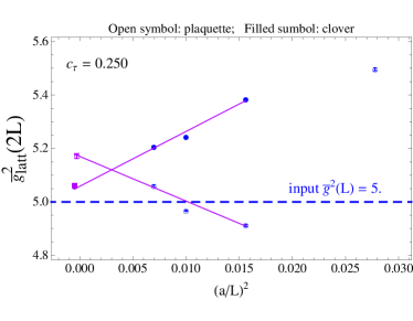
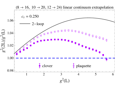
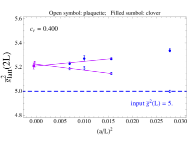
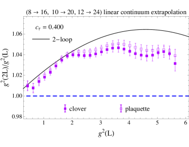
In order to illustrate the dangers of the continuum extrapolation in step scaling studies, I will use some data from these proceedings contribution [28] (see Fig. 1). As we can see, when two different discretizations for the observable $E(x,t)$ are used, the continuum extrapolations of the step scaling function do not agree for small values of the parameter $c$ (Fig. 1 (a)). Note that in this particular case, if one only looks at one observable and only at one value of $c$, it would be difficult to spot the problem. In particular the continuum extrapolations look reasonable even for $c=0.25$. On the other hand for large enough $c\sim 0.4$, both continuum extrapolations agree nicely (Fig. 1 (c)). Figs. 1 (b) and (d) show that the disagreement is larger at strong couplings.

This example illustrates very well the reasons behind the efforts that different groups have put into understanding cutoff effects of flow quantities.

3.1 Tree-level correction

There are many possible choices for lattice gauge actions, but a general class of them can be written symbolically as

$$S({c_{i}})=\frac{1}{g_{0}^{2}}\sum_{x}{\rm Tr}\left(1-c_{0}\raisebox{-5.69046pt}{ \begin{picture}(1.2,1.2)(-0.6,-0.6) \put(-0.5,-0.5){\line(1,0){1.0}} \put(0.5,-0.5){\line(0,1){1.0}} \put(0.5,0.5){\line(-1,0){1.0}} \put(-0.5,0.5){\line(0,-1){1.0}} \put(-0.5,-0.5){\circle*{0.2}} \put(-0.5,0.5){\circle*{0.2}} \put(0.5,-0.5){\circle*{0.2}} \put(0.5,0.5){\circle*{0.2}} \end{picture}}-c_{1}\raisebox{-5.69046pt}{ \begin{picture}(2.2,1.2)(-1.1,-0.6)\put(-1.0,-0.5){\line(1,0){2.0}} \put(-1.0,0.5){\line(1,0){2.0}} \put(-1.0,-0.5){\line(0,1){1.0}} \put(1.0,-0.5){\line(0,1){1.0}} \put(-1.0,-0.5){\circle*{0.2}}\put(0.0,-0.5){\circle*{0.2}}\put(1.0,-0.5){\circle*{0.2}} \put(-1.0,0.5){\circle*{0.2}}\put(0.0,0.5){\circle*{0.2}}\put(1.0,0.5){\circle*{0.2}} \end{picture}}-c_{2}\raisebox{-9.29828pt}{ \begin{picture}(1.7071,1.7071)(-0.7071,-0.7071)\put(0.0,0.0){\line(0,1){1.0}} \put(0.0,1.0){\line(1,0){1.0}} \put(1.0,1.0){\line(0,-1){1.0}} \put(-0.7071,-0.7071){\line(1,0){1.0}} \put(0.0,0.0){\line(-1,-1){0.7071}} \put(1.0,0.0){\line(-1,-1){0.7071}} \put(0.0,0.0){\circle*{0.2}}\put(1.0,0.0){\circle*{0.2}} \put(0.0,1.0){\circle*{0.2}}\put(1.0,1.0){\circle*{0.2}} \put(-0.7071,-0.7071){\circle*{0.2}}\put(0.2929,-0.7071){\circle*{0.2}} \put(0.0,0.0){\circle*{0.03}}\put(0.25,0.0){\circle*{0.03}}\put(0.5,0.0){\circle*{0.03}}\put(0.75,0.0){\circle*{0.03}} \end{picture}}-c_{3}\raisebox{-9.29828pt}{ \begin{picture}(1.7071,1.7071)(-0.7071,-0.7071)\put(-0.7071,-0.7071){\line(0,1){1.0}} \put(0.0,1.0){\line(1,0){1.0}} \put(1.0,1.0){\line(0,-1){1.0}} \put(-0.7071,-0.7071){\line(1,0){1.0}} \put(0.0,1.0){\line(-1,-1){0.7071}} \put(1.0,0.0){\line(-1,-1){0.7071}} \put(-0.7071,-0.7071){\circle*{0.1}} \put(-0.7071,0.2929){\circle*{0.2}} \put(0.0,0.0){\circle*{0.2}}\put(1.0,0.0){\circle*{0.2}} \put(0.0,1.0){\circle*{0.2}}\put(1.0,1.0){\circle*{0.2}} \put(-0.7071,-0.7071){\circle*{0.2}}\put(0.2929,-0.7071){\circle*{0.2}} \put(0.0,0.0){\circle*{0.03}}\put(0.25,0.0){\circle*{0.03}}\put(0.5,0.0){\circle*{0.03}}\put(0.75,0.0){\circle*{0.03}} \put(0.0,0.0){\circle*{0.03}}\put(0.0,0.25){\circle*{0.03}}\put(0.0,0.5){\circle*{0.03}}\put(0.0,0.75){\circle*{0.03}} \put(0.0,0.0){\circle*{0.03}}\put(-0.1768,-0.1768){\circle*{0.03}}\put(-0.3536,-0.3536){\circle*{0.03}}\put(-0.5304,-0.5304){\circle*{0.03}} \end{picture}}\right)\,.$$ (12)

These include the Lüscher-Weisz tree-level improved action ($c_{0}=5/3,c_{1}=-1/12,c_{2}=c_{3}=0$) and the Iwasaki action ($c_{0}=3.648,c_{1}=-0.331,c_{2}=c_{3}=0$).

One has to choose several actions to study a flow quantity, first the action used for the simulation (i.e. to produce the configurations), second the action used in the flow equation (11). Finally, note that $\langle E(x,t)\rangle$ is nothing more than an action density, and therefore, if interested in this observable, any particular discretization of $\langle E(x,t)\rangle$ can be understood as a third choice of action. Each of these actions can be different, and therefore we have several sets of coefficients $c_{i}$: one for the action, one for the flow, and one for the observable.

The influence of these coefficients to tree-level has been clarified recently [26, 27]. The perturbative expansion of our observable of interest reads

$$\langle E(x,t)\rangle=\mathcal{E}_{0}(t,a/L)g^{2}+\mathcal{O}(g^{4})\,,$$ (13)

where $\mathcal{E}_{0}$ can be computed on the lattice. In fact in the case of an infinite lattice we have

$$t^{2}\mathcal{E}_{0}(t,a/L)=\frac{3(N^{2}-1)}{128\pi^{2}}\left\{1+\frac{a^{2}}{t}\left[d^{(o)}-d^{(a)}-3d^{(f)}\right]\right\}+\mathcal{O}(a^{4})\,,$$ (14)

where the coefficients $d^{(o,a,f)}$ parametrize the tree-level cutoff effects produced by the observable discretization, the action used in the simulation and the action used to define the flow respectively. The values of these parameters for some popular choices of discretizations are

$$d^{(o,a,f)}=\left\{\begin{array}[]{l@{\hskip 24pt}l}-1/24\hfil\hskip 24.0&\textrm{plaquette}\\ 1/72\hfil\hskip 24.0&\textrm{L\"{u}scher-Weisz}\\ -5/24\hfil\hskip 24.0&\textrm{Clover}\end{array}\right.\,.$$ (15)

At this point there are some important observations to make

1. The particularly popular choice of using the clover discretization to define flow quantities (couplings, or the scales $t_{0},w_{0},\dots$), does not seem to be a very good idea from the perspective of perturbation theory. This discretization is the one with larger tree-level cutoff effects: 5 times larger than the plaquette definition, and 15 times larger than the Lüscher-Weisz discretization.

2. There is a cancellation between cutoff effects produced by the observable and those produced by the action and the flow. For example the choice of a Wilson action, Wilson flow, and clover observable leads to rather small tree-level cutoff effects. This is due to an accidental cancellation of the cutoff effects produced by the action and flow on one hand, and those of produced by the observable on the other. Note that this accidental cancellation disappears as soon as the setup is changed. For example, using the Symanzik flow and Lüscher-Weisz action, but keeping the clover observable leads to a very poor scenario, with tree-level cutoff effects around 7 times larger.

The perturbative computation of Eq. (14) immediately suggests an improved definition for the coupling

$$g_{\rm GF}^{2}(L)=\hat{\mathcal{N}}^{-1}t^{2}\langle E(x,t)\rangle\Big{|}_{\sqrt{8t}=cL}\,,$$ (16)

where $\hat{\mathcal{N}}=\mathcal{E}_{0}$ (i.e. Using the tree-level lattice computation instead of the continuum result to define the coupling). This definition of the coupling has no cutoff effects to tree-level, and has been used in most step scaling studies (see [11, 12, 13, 28, 29]). The exception were the studies using periodic boundary conditions (like [10, 30, 31]), or smeared gauge actions (for example [34]), since the perturbative computation in these setups is more involved (see the recent work [26] for the case of periodic boundary conditions).

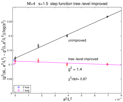
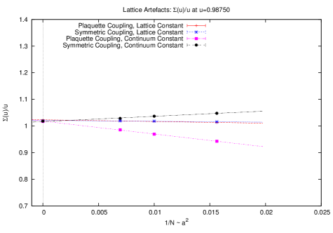
This improved definition of the coupling has a big impact on the cutoff effects. A nice example is given in [26], where the step-scaling study of [10] is repeated with the improved definition of the coupling Eq. (16). The result can be seen in Fig. 2. This example is specially impressive, partially because the original data of [10] has a choice of discretizations (Lüscher-Weisz action, Symanzik flow and Clover observable) that, as we have commented, make the tree-level correction specially large.

Figure 2: Comparison of the continuum extrapolation of the step scaling function of the coupling defined with the continuum norm and the tree-level improved definition. (Source [26]).

The work [10] also proposes to use a general class of actions given by Eq. (12) setting $c_{2}=c_{3}=0$. Since the two remaining coefficients are related by $c_{0}+8c_{1}=1$, each choice of action has one free parameter, resulting in three parameters that can be chosen arbitrarily. The concrete proposal is to choose them to cancel the tree-level cutoff effects of $\langle E(x,t)\rangle$ in infinite volume to order $a^{2},a^{4}$ and $a^{6}$. It is the opinion of the author that this criteria to choose the coefficients is not very appealing, especially taking into account that one can remove all the tree-level cutoff effects (to all orders in $a$) with the simple coupling definition of Eq.(16), and there is no good reason to think that this choice of coefficients will result in reduced cutoff effects for any other quantity or to higher orders in $g_{0}$.

3.2 Phenomenological improvement

In any $\mathcal{O}(a)$ improved setup, the lattice gradient flow coupling can be expanded as

$$g_{\rm GF}^{2}(L;a/L)=\mathcal{N}^{-1}t^{2}\langle E(x,t)\rangle\Big{|}_{\sqrt{8t}=cL}=g_{\rm GF}^{2}(L;0)+\left(\frac{a}{L}\right)^{2}A(c,L)+\mathcal{O}(a^{4})\,,$$ (17)

where, as we have seen in the previous section, $A(c,L)$ depends not only on the volume and the parameter $c$, but also on the choice of boundary conditions, the action, the flow, etc…The proposal of [30] is to subtract the cutoff effects $a^{2}A(c,L)$ by modifying the definition of the coupling to

$$\tilde{g}_{\rm GF}^{2}(L;a/L)=\mathcal{N}^{-1}t^{2}\langle E(x,t+a^{2}\tau)\rangle\Big{|}_{\sqrt{8t}=cL}\,.$$ (18)

The parameter $\tau$ is chosen to cancel the leading cutoff effects. One can see this $t$-shift as adding an $a^{2}$ term to the coupling definition

$$\tilde{g}_{\rm GF}^{2}(L;a/L)=g_{\rm GF}^{2}(L;a/L)+\frac{a^{2}\tau}{\mathcal{N}}\langle t^{2}\partial_{t}E(x,t)\rangle\Big{|}_{\sqrt{8t}=cL}+\mathcal{O}(a^{4})\,.$$ (19)

Recently a similar approach in spirit has been taken in [32]. In this case instead of canceling the $\mathcal{O}(a^{2})$ term by a shift in the flow time, the authors use a linear combination of the coupling defined with different discretizations of the observable

$$\tilde{g}_{\rm GF}^{2}(L;a/L)=Xg_{\rm GF;Clover}^{2}(L;a/L)+(1-X)g_{\rm GF;Plaquette}^{2}(L;a/L)\,,$$ (20)

where the parameter $X$ is chosen to eliminate the leading cutoff effects.

Obviously these are always legitimate things to do, that cannot change the values obtained after a properly done continuum extrapolation. In this context one should avoid giving a dependence to $\tau$ or $X$ on the bare parameters (like $\beta$), since this would result in a different $a^{2}$ shift for each value of $a$, and could give the wrong continuum extrapolations. One should also be careful with extrapolating to the continuum with a constant fit, even if the data “looks flat” after having applied the correction, since one could artificially reduce the statistical error of the extrapolation. Fig. 3 shows how different values of $\tau$ results in data with different cutoff effects, but whose continuum extrapolations are in agreement. Moreover these recipes are simple to implement since the integration of the flow equations naturally gives $\langle E(x,t)\rangle$ at many values of $t$, and the evaluation of a different observable is always cheap.

(a)

(b)

Figure 3: Left: Continuum extrapolation of the step-scaling function for different values of $\tau$

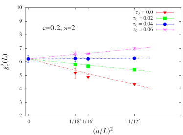
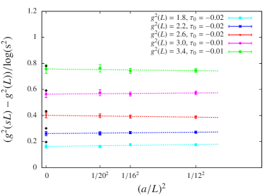
In the opinion of the author the weak point of these approaches is that the improvement of flow quantities requires one to improve the flow equation, the discretization of the observable and the action used to generate the configurations [8, 27]. A single parameter ($\tau$ or $X$) is not able to achieve this effect and this translates in $\tau$ (or $X$) being a function of everything: choice of boundary conditions, choice of action (both gauge and fermionic), volume, etc…The dependence of this parameter on these details is not small (see for example Fig. 3, where $\tau$ changes by 100% when the renormalized coupling changes in the range $\sim 2-4$). In the end $\tau$ (or $X$) cannot be computed analytically nor by studying other flow quantities, but has to be inferred from the same data that one is trying to improve.

3.3 Symanzik improvement and the Zeuthen flow

A very appealing approach to systematically reduce cutoff effects is the Symanzik improvement program. Its purpose is far more ambitious than looking for an accidental cancellation between cutoff effects for some particular observable. When we choose a particular discretization (to define an action/observable) we are choosing what our theory looks like at very high energy scales (the cutoff $1/a$). The idea of the Symanzik improvement program is to choose these discretizations so that the effective theory at energy scales much smaller than the cutoff looks as close as possible to the continuum theory. This program starts by describing a particular lattice action $S_{\rm latt}$ by an effective continuum theory. For example for pure gauge theories any lattice action can be described by an effective action given by

$$S_{\rm eff}=S_{\rm YM}+a^{2}S_{2}+a^{4}S_{4}+\dots\,,$$ (21)

(i.e. any choice of actions will have the Yang-Mills action as first approximation $S_{\rm YM}$, but different discretizations will produce different cutoff effects described by $S_{2},S_{4},\dots$). Symanzik’s idea was to choose a discretization such that the effective continuum description has some of these terms absent (i.e. $S_{2}=0$).

We can say that the basic idea behind Symanzik improvement program is to help us choosing a discretization that represents better continuum physics. Being a choice made at the cutoff scale $1/a$, it should be obvious that improvement parameters can not depend on the boundary conditions, the volume, or the choice of observable. In other words, if one finds the Symanzik improved action, this is valid for all observables (this includes all values of the parameter $c$ that defines the coupling), all volumes, all boundary conditions,etc…

The application of the Symanzik improvement program to the gradient flow has to be done using a 5D local field theory [6], in which the flow time becomes the fifth coordinate with values in the positive real axis. The action in the continuum Euclidean space can be written as

$$S^{\rm cont}=-\frac{1}{2g_{0}^{2}}\int{\rm d}^{4}x\,{\rm Tr}\left\{F_{\mu\nu}F_{\mu\nu}\right\}-2\int_{0}^{\infty}{\rm d}t\int{\rm d}^{4}x\,{\rm Tr}\left\{{L_{\mu}(x,t)}[\partial_{t}B_{\mu}(x,t)-D_{\nu}G_{\nu\mu}]\right\}\,,$$ (22)

where $F_{\mu\nu}$ and $G_{\mu\nu}$ are the field strength at $t=0$ and $t>0$ respectively. $L_{\mu}(x,t)$ is a Lagrange multiplier in the sense that the path integral over this field imposes the flow equation (1) in the bulk of the 5D space (i.e. for $t>0$).

The main point is that due to the classical nature of the theory at $t>0$, one can completely eliminate all (i.e. to all orders in the coupling) $\mathcal{O}(a^{2})$ cutoff effects in the bulk [27]. Making a long story short, this non-perturbative improvement is achieved by using the Zeuthen flow to integrate the flow equations

$$a^{2}\partial_{t}V_{\mu}(x,t)=-g_{0}^{2}\left[\left(1+\frac{a^{2}}{12}D_{\mu}D_{\mu}^{*}\right)T^{a}\partial_{x,\mu}^{a}S_{\rm LW}(V)\right]V_{\mu}(x,t)\,,$$ (23)

where $D_{\mu}$ and $D_{\mu}^{*}$ are the forward and backward lattice covariant derivatives, and $S_{\rm LW}$ is the tree-level Lüscher-Weisz improved action (i.e. Eq.(12) with $c_{0}=5/3,c_{1}=-1/12,c_{2}=c_{3}=0$). In the same way one can define clasically improved discretizations for observables (like $E(x,t)$), that will not introduce any $\mathcal{O}(a^{2})$ discretization effects.

In summary, from the three discretization choices that one has to make in order to study any flow quantity, the Symanzik improvement program gives a way to fix the discretization used to integrate the flow equation and to evaluate flow observables, so that no $\mathcal{O}(a^{2})$ effects are introduced. The remaining cutoff effects are only those of the action used to produce the configurations and a couple of boundary counterterms.

4 Some recent results

Since the proposal of using the gradient flow to define a renormalized coupling there have been several works using this technique to investigate the dynamics of strongly coupled non-abelian gauge theories. Most of the applications are related to models beyond QCD and the search for an infrared fixed-point (see for a recent review [33]). On the other hand, the gradient flow has been used in QCD mainly for scale setting (see [8]). We have already mentioned some of the recent works in the previous sections. In this section we will briefly mention other works paying attention to the details discussed in earlier sections. The reader interested in a more exhaustive review of the recent works should also consult [33].

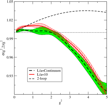
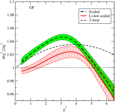
The work [34] studies the running of the coupling in the minimal technicolor model ($SU(2)$ gauge group with two adjoint fermions) using both the Schrödinger functional coupling and the gradient flow coupling. Both schemes show an IR fixed point (see Fig 4) at quite different values of the coupling. Of course since the schemes are different there is no reason to expect the values of the coupling at the fixed point to be the same. This work uses a smeared gauge action, which modifies the lattice leading order value of $t^{2}\langle E(x,t)\rangle$. The improved coupling definition Eq.(16) cannot be used without an analytic computation. The authors address the issue of large cutoff effects by using a large value of $c$

(a)

(b)

Figure 4: Step scaling function in the minimal walking technicolor in two different schemes. Left: $\sigma_{2}(g^{2}_{\rm SF})/g_{\rm SF}^{2}$ in the SF scheme, showing an IR fixed point at $g^{2}_{\rm SF}\sim 2$. Right: $\sigma_{2}(g^{2}_{\rm GF})/g_{\rm GF}^{2}$ in the gradient flow scheme, showing an IR fixed point at $g^{2}_{\rm GF}\sim 5$. (Source [34])

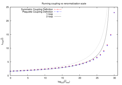
Computing non-perturbative effects in $SU(N)$ gauge theories in the large $N$ ’t Hooft limit (keeping $\lambda=g^{2}N$ constant) via lattice techniques is a difficult task because the number of degrees of freedom that have to be simulated on a computer increase with $N$. Nevertheless, using the ideas of volume independence (see [35] for a recent review), the authors of [29] have computed the running of the t’Hooft coupling Fig. 5. The authors use the tree-level corrected coupling definition Eq. (16) and the clover and plaquette definitions of the observable to estimate the systematic of the continuum extrapolations. Their results also indicate that the tree-level corrected definition of the coupling Eq. (16) has a big impact in the cutoff effects.

(a)

(b)

Figure 5: Left: Continuum extrapolation of the step scaling function of the t’Hooft coupling in $SU(\infty)$. Right: Running of the t’Hooft coupling $\lambda=Ng^{2}$ in $SU(\infty)$ gauge theory (source [29]).

5 Fermion flow and renormalization of composite operators

The flow can also be introduced for the fermion fields [6]

$$\partial_{t}\chi(x,t)=D_{\mu}D_{\mu}\chi(x,t)\,,$$ (24)

where $D_{\mu}=\partial_{\mu}+B_{\mu}$, and the fermion flow field obeys the initial condition $\chi(x,t)|_{t=0}=\psi(x)$. In this case the fermion flow field requires renormalization, but there is no operator mixing at positive flow time. i.e. composite fermion operators renormalize multiplicatively at positive flow time.

In fact the study of Ward Identities at positive flow time has lead to a novel approach to the renormalization of some composite operators. We have recently seen the cases of the axial current, the chiral condensate [6, 36], or the energy momentum tensor [37].

On the other hand the so called small flow-time expansion offers the possibility of a general approach to the renormalization of a generic composite operator $O(x,t)$. When the flow time is taken to zero $O(x,t)$ has to converge to the bare operator $O(x)$. Since the latter usually requires renormalization, $O(x,t)$ becomes singular when taking the $t\rightarrow 0$ limit in a way that can be expressed as an asymptotic expansion in renormalized operators with singular coefficients [5]

$$O(x,t)=\sum_{\alpha}c_{\alpha}(t)O_{\rm R}^{\alpha}(x)+\mathcal{O}(t)\,.$$ (25)

The previous sum runs over all the operators of dimension smaller that the dimension of $O(x,t)$ and compatible with its continuum symmetries. We can use $E(x,t)=-\frac{1}{4}{\rm Tr}(G_{\mu\nu}G_{\mu\nu})$, as an example, whose small flow time expansion reads

$$E(x,t)=c_{1}(t)\mathbf{1}+c_{2}(t)\{F_{\mu\nu}F_{\mu\nu}\}_{\rm R}(x)+\mathcal{O}(t)\,.$$ (26)

In this example, $E(x,t)$ mixes with the vacuum and with the renormalized action density. In fact this relation can be used to determine the spin-0 component of the energy-momentum tensor [38]

$$\{T_{\mu\mu}\}_{\rm R}(x)=\{F_{\mu\mu}F_{\mu\mu}\}_{\rm R}(x)=\lim_{t\rightarrow 0}c_{2}^{-1}(t)\left\{E(x,t)-\langle E(x,t)\rangle\right\}\,.$$ (27)

This relation holds in the continuum, and its use in the lattice framework requires that the continuum limit is taken before the $t\rightarrow 0$ limit. This means that the scale given by the flow time has to be large compared with the lattice spacing, and small compared with any other relevant scale of the problem (i.e. $a\ll\sqrt{8t}\ll L,\Lambda,T$).

Moreover one needs to compute the small flow time coefficients $c_{\alpha}(t)$. Ref. [38] proposes to use perturbation theory. This proposal has recently been used to extract thermodynamic quantities (see the contribution of this conference [7] for more details). Generally speaking there might be concerns about using leading order perturbation theory at energy scales below the lattice cutoff $1/a$, and this is the reason why we have seen different works focused on the non-perturbative determination of the small flow time coefficients. The authors of [39] propose to determine non-perturbatively the quantity $\gamma_{\alpha}(t)=-2t\frac{d}{dt}\log c_{\alpha}(t)$ and then construct $c_{\alpha}(t)$ by integrating using perturbation theory as initial condition. The functions $\gamma_{\alpha}(t)$ can be extracted from correlation functions. For example in the case mentioned before we have

$$\gamma_{2}(t)=-2t\frac{d}{dt}\log\langle E(x,t)E(x,s)\rangle_{\rm connected}+\mathcal{O}(t)\,.$$ (28)

Although the idea is appealing, and has the advantage that it can be generally applicable to any composite operator with a complicated mixing pattern (including fermion composite operators), it remains to be seen how well it actually works in a concrete numerical example.

We have also seen how the small flow-time expansion can be used to compute the strange content of the nucleon [40]. In this case we consider the connected part of the scalar strange density $\overline{s}s(x,t)$ in a nucleon state

$$O^{\rm sub}(x,t)=N\,\overline{s}s(x,t)\,N^{\dagger}-\langle NN^{\dagger}\rangle\langle\overline{s}s(x,t)\rangle\,,$$ (29)

where $N$ is a nucleon interpolating operator. The small flow time expansion of this operator reads

$$O^{\rm sub}(x,t)=c_{3}(t)O^{\rm sub}(x,0)+\mathcal{O}(t)\,,$$ (30)

and $c_{3}(t)$ can be determined from the Ward identities (see [40] for more details).

6 Conclusions

We have seen in the recent years a growing interest in the gradient flow as a tool for scale setting and to define renormalized couplings. In this contribution we have reviewed the main ideas behind these applications putting a strong emphasis on the role of the continuum extrapolation and cutoff effects of flow quantities. We have also commented on the use of the small flow-time expansion as a general tool to renormalize composite operators, a very interesting and promising application where there is still a lot of work to do.

I would like to conclude with a brief comment on some recent works that I did not have time to cover or did not fit in the presentation, but nevertheless I found interesting. Perturbative computations have proven to be a useful tool (i.e. to understand the structure of cutoff effects), but also perturbative computations of flow quantities are usually tedious. The application of numerical stochastic perturbation theory for flow quantities [41] is an interesting idea. The use of the gradient flow to extract matrix elements non-perturbatively with a simplified mixing pattern has also been considered recently [42], and shows a promising future.

References

- [1] R. Narayanan and H. Neuberger, Infinite N phase transitions in continuum Wilson loop operators, JHEP 0603 (2006) 064, [hep-th/0601210].
- [2] M. Lüscher, Trivializing maps, the Wilson flow and the HMC algorithm, Commun.Math.Phys. 293 (2010) 899–919, [arXiv:0907.5491].
- [3] R. Lohmayer and H. Neuberger, Continuous smearing of Wilson Loops, PoS LATTICE2011 (2011) 249, [arXiv:1110.3522].
- [4] M. Lüscher, Properties and uses of the Wilson flow in lattice QCD, JHEP 1008 (2010) 071, [arXiv:1006.4518].
- [5] M. Lüscher and P. Weisz, Perturbative analysis of the gradient flow in non-abelian gauge theories, JHEP 1102 (2011) 051, [arXiv:1101.0963].
- [6] M. Luscher, Chiral symmetry and the Yang–Mills gradient flow, JHEP 1304 (2013) 123, [arXiv:1302.5246].
- [7] M. Kitazawa, M. Asakawa, T. Hatsuda, T. Iritani, E. Itou, et al., Measurement of thermodynamics using gradient flow, arXiv:1412.4508.
- [8] R. Sommer, Scale setting in lattice QCD, PoS LATTICE2013 (2014) 015, [arXiv:1401.3270].
- [9] M. Lüscher, P. Weisz, and U. Wolff, A Numerical method to compute the running coupling in asymptotically free theories, Nucl.Phys. B359 (1991) 221–243.
- [10] Z. Fodor, K. Holland, J. Kuti, D. Nogradi, and C. H. Wong, The Yang-Mills gradient flow in finite volume, JHEP 1211 (2012) 007, [arXiv:1208.1051].
- [11] P. Fritzsch and A. Ramos, The gradient flow coupling in the Schrödinger Functional, JHEP 1310 (2013) 008, [arXiv:1301.4388].
- [12] A. Ramos, The gradient flow running coupling with twisted boundary conditions, JHEP 1411 (2014) 101, [arXiv:1409.1445].
- [13] M. Lüscher, Step scaling and the Yang-Mills gradient flow, JHEP 1406 (2014) 105, [arXiv:1404.5930].
- [14] K. Symanzik, Schrodinger Representation and Casimir Effect in Renormalizable Quantum Field Theory, Nucl.Phys. B190 (1981) 1.
- [15] M. Lüscher, R. Narayanan, P. Weisz, and U. Wolff, The Schrödinger Functional: a renormalizable probe for non-abelian gauge theories, Nucl.Phys. B384 (1992) 168–228, [hep-lat/9207009].
- [16] S. Sint, On the Schrödinger functional in QCD, Nucl.Phys. B421 (1994) 135–158, [hep-lat/9312079].
- [17] S. Sint, The Chirally rotated Schrödinger functional with Wilson fermions and automatic O(a) improvement, Nucl.Phys. B847 (2011) 491–531, [arXiv:1008.4857].
- [18] R. Frezzotti and G. Rossi, Chirally improving Wilson fermions. 1. O(a) improvement, JHEP 0408 (2004) 007, [hep-lat/0306014].
- [19] A. Gonzalez-Arroyo, J. Jurkiewicz, and C. Korthals-Altes, Ground state metamorphosis for Yang-Mills fields on a finite periodic lattice, Freiburg ASI 1981:0339 (1981).
- [20] L. Del Debbio, G. M. Manca, and E. Vicari, Critical slowing down of topological modes, Phys.Lett. B594 (2004) 315–323, [hep-lat/0403001].
- [21] ALPHA Collaboration, S. Schaefer, R. Sommer, and F. Virotta, Critical slowing down and error analysis in lattice QCD simulations, Nucl. Phys. B845 (2011) 93–119, [arXiv:1009.5228].
- [22] P. Fritzsch, A. Ramos, and F. Stollenwerk, Critical slowing down and the gradient flow coupling in the Schrödinger functional, PoS Lattice2013 (2013) 461, [arXiv:1311.7304].
- [23] P. Fritzsch and A. Ramos, Studying the gradient flow coupling in the Schr dinger functional, PoS Lattice2013 (2014) 319, [arXiv:1308.4559].
- [24] ALPHA Collaboration, G. de Divitiis et al., Universality and the approach to the continuum limit in lattice gauge theory, Nucl.Phys. B437 (1995) 447–470, [hep-lat/9411017].
- [25] M. D. Brida, P. Fritzsch, T. Korzec, A. Ramos, S. Sint, et al., Towards a new determination of the QCD Lambda parameter from running couplings in the three-flavour theory, PoS LATTICE2014 (2014) 291, [arXiv:1411.7648].
- [26] Z. Fodor, K. Holland, J. Kuti, S. Mondal, D. Nogradi, et al., The lattice gradient flow at tree-level and its improvement, JHEP 1409 (2014) 018, [arXiv:1406.0827].
- [27] A. Ramos and S. Sint, On effects in gradient flow observables, arXiv:1411.6706.
- [28] C. J. D. Lin, K. Ogawa, H. Ohki, A. Ramos, and E. Shintani, SU(3) gauge theory with 12 flavours in a twisted box, arXiv:1410.8824.
- [29] M. Garc a P rez, A. Gonz lez-Arroyo, L. Keegan, and M. Okawa, The twisted gradient flow running coupling, JHEP 1501 (2015) 038, [arXiv:1412.0941].
- [30] A. Cheng, A. Hasenfratz, Y. Liu, G. Petropoulos, and D. Schaich, Improving the continuum limit of gradient flow step scaling, JHEP 1405 (2014) 137, [arXiv:1404.0984].
- [31] A. Hasenfratz, D. Schaich, and A. Veernala, Nonperturbative beta function of eight-flavor SU(3) gauge theory, arXiv:1410.5886.
- [32] Z. Fodor, K. Holland, J. Kuti, S. Mondal, D. Nogradi, et al., The running coupling of 8 flavors and 3 colors, arXiv:1503.0113.
- [33] Y. Aoki, Near conformal strong dynamics, Talk at The 32nd International Symposium on Lattice Field Theory (2014).
- [34] J. Rantaharju, The Gradient Flow Coupling in Minimal Walking Technicolor, PoS Lattice2013 (2014) 084, [arXiv:1311.3719].
- [35] M. G. Perez, A. Gonzalez-Arroyo, and M. Okawa, Volume independence for Yang-Mills fields on the twisted torus, arXiv:1406.5655.
- [36] A. Shindler, Chiral Ward identities, automatic O(a) improvement and the gradient flow, Nucl.Phys. B881 (2014) 71–90, [arXiv:1312.4908].
- [37] L. Del Debbio, A. Patella, and A. Rago, Space-time symmetries and the Yang-Mills gradient flow, JHEP 1311 (2013) 212, [arXiv:1306.1173].
- [38] H. Suzuki, Energy-momentum tensor from the Yang-Mills gradient flow, PTEP 2013 (2013), no. 8 083B03, [arXiv:1304.0533].
- [39] A. Patella, Energy-momentum tensor on the lattice and Wilson flow., Talk at The 32nd International Symposium on Lattice Field Theory (2014).
- [40] A. Shindler, J. de Vries, and T. Luu, Beyond-the-Standard-Model matrix elements with the gradient flow, PoS LATTICE2014 (2014) 251, [arXiv:1409.2735].
- [41] M. Dalla Brida and D. Hesse, Numerical Stochastic Perturbation Theory and the Gradient Flow, PoS Lattice2013 (2014) 326, [arXiv:1311.3936].
- [42] C. Monahan and K. Orginos, Locally smeared operator product expansions in scalar field theory, arXiv:1501.0534.