Photogalvanic effect in HgTe/CdTe topological insulator due to edge-bulk optical transitions

Abstract

We study theoretically 2D HgTe/CdTe quantum well topological insulator (TI) illuminated by circularly polarized light with frequencies higher than the difference between the equilibrium Fermi level and the bottom of the conduction band (THz range). We show that electron-hole asymmetry results in spin-dependent electric dipole transitions between edge and bulk states, and we predict an occurrence of a circular photocurrent. If the edge state is tunnel-coupled to a conductor, then the photocurrent can be detected by measuring an electromotive force (EMF) in the conductor, which is proportional to the photocurrent.

I Introduction

Topological insulators (TIs) became a focus of attention of many condensed matter physicists in recent years, not least due to their possible applications in spintronics and quantum computing. These are materials with time-reversal symmetry and non-trivial topological order, which have an insulating bulk but conducting topologically protected edge/surface states König et al. (2008); Hasan and Kane (2010); Qi and Zhang (2011). Spin-orbit interaction plays a significant role in these materials, and particularly manifests itself in spin-momentum locking of charge carriers in edge/surface states.

Optical excitation is an efficient tool for generating currents in materials. This process has been studied in 3D TIs Muniz and Sipe (2014); McIver et al. (2012); Misawa et al. (2011); Junck et al. (2013); Hosur (2011); Jozwiak et al. (2013); Zhang et al. (2010); Park and Louie (2012); Wu et al. (2012); Zhu et al. (2014); Li and Carbotte (2013); Wilson et al. (2014). In Ref. Muniz and Sipe, 2014 effects in study are due to electric optical transitions between surface states, which are possible in the presence of magnetic field. Besides, in the presence of strong magnetic fields, the electric dipole transitions between Landau levels are also possible Li and Carbotte (2013). In contrast to these papers, here we study 2D TIs and show that the optical generation of the current is possible without magnetic field as well.

HgTe/CdTe quantum well structures Bernevig et al. (2006) are one of the most well-known 2D TIs. These quantum wells exhibit an inverted band structure if their width exceeds a certain critical value. The inverted band structure and strong spin-orbit interaction give rise to unusual optoelectronic phenomena, e.g. a nonlinear magneto-gyrotropic photogalvanic effect (PGE) Diehl et al. (2009) (PGE). A circular PGE was also experimentally observed Wittmann et al. (2010) when the sample was illuminated by mid-infrared or terahertz laser radiation. These photocurrents were induced due to direct transitions between different size-quantized subbands or due to indirect (Drude-like) transitions within the lowest size-quantized subband. In both cases the optical transitions responsible for the PGE involve only bulk states. However, in the case of a finite sample size of 2D TI there exist topologically protected helical edge states which form two branches with opposite spins Bernevig et al. (2006). In the recent paper Scharf et al. (2015) it was predicted that edge states affect bulk magneto-conductivity. The paper focuses on the bulk properties in a strong magnetic field and does not discuss optoelectronic properties of the edge states. However, it is of interest whether the photocurrent can be induced at the edge states at zero magnetic field. A PGE due to transitions between edge states of the opposite chiralities has been predicted in Ref. Artemenko and Kaladzhyan, 2013, but electric dipole transitions between them are forbidden by selection rules, and only magnetic dipole transitions are possible in this case. Thus, the direct transitions between the edge states are weak. Unlike Ref. Artemenko and Kaladzhyan, 2013, in this paper we study electric dipole transitions between the edge and bulk states in HgTe/CdTe quantum well 2D TI in zero magnetic field, which lead to the edge currents. To our knowledge, this mechanism of the PGE in TI has not been studied yet.

Starting from the Bernevig-Hughes-Zhang (BHZ) model of HgTe/CdTe 2D TI, we find a relation between matrix elements of the edge-bulk transitions. In the general case the electron-hole symmetry is broken, and the probability of transition depends on the spin and, hence, on the chirality. Thus, the transitions will lead to a different population of spin-up and spin-down states and to occurrence of a photoinduced electric current. In order to study this effect, we derive a kinetic equation and then solve it in the quasi-equilibrium approximation. We also propose a way to detect the photoinduced current by coupling 2D TI with a conductor and measuring an electromotive force (EMF) induced in the conductor.

The paper is organized as follows. In Section II we consider optical transitions between edge and bulk states and derive the photoinduced electric current. In section III we calculate the EMF that appears in the conductor tunnel-coupled to the edge state.

Below we set $\hbar=1$, $c=1$.

Figure 1: Schematic picture of optical transitions between two edge state branches and bulk states. Circularly polarized light of frequency $\omega_{0}$ exceeding the absorption threshold by $\Delta\omega$ induces transitions between edge and bulk conduction band states. The different thickness of arrows depicts that probability of electric dipole transitions may depend on chirality/spin of the edge electron.

II Optical transitions between edge and bulk states

We consider a HgTe/CdTe quantum well TI with a conducting helical edge state illuminated by circularly polarized light with a frequency $\omega_{0}$ slightly exceeding the the absorption threshold, so that optical transitions may occur between the edge state and the bulk conduction band (Fig. 1). We assume that the TI is located at $x>0$; $y$-axis is taken along the edge of TI, and $z$-axis is perpendicular to the 2D TI.

Both in HgTe and CdTe the relevant bands are s-type band ($\Gamma_{6}$) and p-type band split by spin-orbit interaction into a $J=3/2$ ($\Gamma_{8}$) and a $J=1/2$ ($\Gamma_{7}$) bands. The latter is usually neglected as it has negligible effects on the band structure Bernevig et al. (2006); Novik et al. (2005). CdTe has a band-ordering similar to GaAs with $\Gamma_{6}$ conduction band and $\Gamma_{8}$ valence band. In HgTe the usual band-ordering is inverted. The quantum well subbands derived from the heavy-hole $\Gamma_{8}$ are usually denoted by $H_{n}$, and the subbands derived from the electron $\Gamma_{6}$ are denoted by $E_{n}$.

We describe HgTe/CdTe quantum well TI by the four-band BHZ model Bernevig et al. (2006).

In the four-component basis consisting of $\left|E_{1}\uparrow\right\rangle$, $\left|H_{1}\uparrow\right\rangle$, $\left|E_{1}\downarrow\right\rangle$, $\left|H_{1}\downarrow\right\rangle$ with $m_{J}=1/2,3/2,-1/2,-3/2$ correspondingly, the Hamiltonian reads:

$$\hat{H}_{BHZ}=-\mathcal{D}\hat{\mathbf{k}}^{2}+\\ \begin{pmatrix}\mathcal{M}-\mathcal{B}\hat{\mathbf{k}}^{2}&\mathcal{A}\hat{k}_{+}&0&0\\ \mathcal{A}\hat{k}_{-}&-(\mathcal{M}-\mathcal{B}\hat{\mathbf{k}}^{2})&0&0\\ 0&0&\mathcal{M}-\mathcal{B}\hat{\mathbf{k}}^{2}&-\mathcal{A}\hat{k}_{-}\\ 0&0&-\mathcal{A}\hat{k}_{+}&-(\mathcal{M}-\mathcal{B}\hat{\mathbf{k}}^{2})\end{pmatrix},$$ (1)

where $\hat{k}_{\pm}=\hat{k}_{x}\pm i\hat{k_{y}}$. Here $\mathcal{A}$, $\mathcal{B}$, $\mathcal{D}$, $\mathcal{M}$ are material parameters, which depend on quantum well geometry: $\mathcal{A}>0$, $\mathcal{B}<0$; parameter $\mathcal{M}$ is negative if the quantum well is in a TI state, and $2|\mathcal{M}|$ is a value of a band gap in TI. Parameter $\mathcal{D}\neq 0$ if electron-hole symmetry is broken, and $D=0$ otherwise.

Since the Hamiltonian (1) has been obtained in kp-approximation, and the non-diagonal part of (1) linear by quasi-momentum $\hat{\mathbf{k}}$ corresponds to kp-term, the Hamiltonian of a light-matter interaction in electric dipole approximation reads

$$\hat{H}_{e-A} =\;\hat{H}_{1}\left({{A}}_{x}-i{{A}}_{y}\right)+\hat{H}_{1}^{\dagger}\left({{A}}_{x}+i{{A}}_{y}\right)$$ (2)

$$\hat{H}_{1} =\;|e|\left|H_{1}\uparrow\right\rangle\left\langle E_{1}\uparrow\right|-|e|\left|E_{1}\downarrow\right\rangle\left\langle H_{1}\downarrow\right|$$ (3)

where $e$ is the electron charge, $\mathbf{{A}}$ is a vector-potential of electromagnetic field. In the case of right-hand polarized light (as defined from the point of view of the source) propagating along $z$-axis the vector-potential can be represented as

$${{A}}_{x}=\frac{\sqrt{4\pi\mathcal{W}}}{n_{r}\omega_{0}}\cos\omega_{0}t,\quad{{A}}_{y}=-\frac{\sqrt{4\pi\mathcal{W}}}{n_{r}\omega_{0}}\sin\omega_{0}t,\quad{{A}}_{z}=0,$$ (4)

where $\mathcal{W}$ is the intensity of light, $n_{r}$ is the refractive index.

Under the illumination by the right-hand circularly polarized light the selection rules allow only those electric dipole transitions from the edge to bulk, which increase angular momentum by $\hbar$. In the Hamiltonian (2) these transitions are described by the first term. The conjugate term describes the reverse optical transitions.

In the absence of the boundary, the eigen states of 2D TI are bulk states separated by a gap, and the bulk states at the bottom of the conduction band are formed by $H_{1}$ states with a zero momentum and a well-defined projection of an angular momentum $m_{J}=\pm 3/2$.

In a finite-size sample, there appear edge states which are superpositions of $E_{1}$ and $H_{1}$ Bloch wavefunctions. These edge states can be found by solving Schroedinger equation with zero boundary conditions for the Hamiltonian (1) in the coordinate representation in $x$-direction and the momentum representation in $y$-direction (see Ref. Zhang et al., 2009):

$$\psi_{edge,s}\propto\left(is\sqrt{|\mathcal{B}-\mathcal{D}|}\left|E_{1},s\right\rangle+\sqrt{|\mathcal{B}+\mathcal{D}|}\left|H_{1},s\right\rangle\right)\times\\ \left(e^{-\lambda_{s,-}x}-e^{-\lambda_{s,+}x}\right),$$ (5)

where $\lambda_{s,\pm}$ are inverse decay lengths for the localized edge states.

In the presence of the boundary, conduction band wavefunctions are distorted near the boundary where they overlap with the edge states. Instead of explicitly calculating the conduction band wavefunctions by solving Schroedinger equation with zero boundary conditions, we will use the time-reversal symmetry and orthogonality conditions for the eigen states of the Hamiltonian.

The BHZ Hamiltonian and zero boundary condition are invariant under the time-reversal symmetry $\hat{\Theta}$. Therefore, if the spin-up eigen state with energy $\epsilon$ is of the form $\Psi_{bulk,\uparrow}(\epsilon,k_{y},x)=f_{\epsilon,k_{y}}(x)\left|E\uparrow\right\rangle+g_{\epsilon,k_{y}}(x)\left|H\uparrow\right\rangle$, then the spin-down eigen state can be obtained as

$$\hat{\Theta}\Psi_{bulk,\uparrow}=-f^{*}_{\epsilon,-k_{y}}(x)\left|E_{1}\downarrow\right\rangle-g^{*}_{\epsilon,-k_{y}}(x)\left|H_{1}\downarrow\right\rangle$$

We denote the overlap integrals between the edge and bulk states as:

$$F(\epsilon,k_{y}) =\int\limits_{0}^{+\infty}\left(e^{-\lambda_{-}x}-e^{-\lambda_{+}x}\right)f_{\epsilon,k_{y}}(x)dx,$$

$$G(\epsilon,k_{y}) =\int\limits_{0}^{+\infty}\left(e^{-\lambda_{-}x}-e^{-\lambda_{+}x}\right)g_{\epsilon,k_{y}}(x)dx.$$

Mutual orthogonality of edge and bulk states yields the relation between the integrals

$$\frac{F}{G}=-i\frac{\sqrt{|\mathcal{B}+\mathcal{D}|}}{\sqrt{|\mathcal{B}-\mathcal{D}|}}.$$ (6)

Thus, both $f$ and $g$ are non-zero, and not only the edge states are superpositions of $E$ and $H$ Bloch wavefunctions with different well-defined projections of total angular momentum, but the bulk conduction states are also their superpositions even at the bottom of the band. Selection rules allow transitions from $\left|E\uparrow\right\rangle$ to $\left|H\uparrow\right\rangle$, and from $\left|H\downarrow\right\rangle$ to $\left|E\downarrow\right\rangle$. Thus, the transitions from the both edge state branches to the conduction band satisfy the selection rules. Calculation of the matrix elements $w_{s}$ of the first term of the Hamiltonian (2) corresponding to these transitions yields the main relation

$$\frac{|w_{\downarrow}|}{|w_{\uparrow}|}=\frac{\sqrt{|\mathcal{B}-\mathcal{D}|}|G|}{\sqrt{|\mathcal{B}+\mathcal{D}|}|F|}=\frac{\mathcal{B}-\mathcal{D}}{\mathcal{B}+\mathcal{D}}.$$ (7)

Note, that if electron-hole symmetry is present, the probabilities of optical transitions from the both edge state branches are equal. Electron-hole symmetry implies that the edge states are superpositions of $\left|E,s\right\rangle$ and $\left|H,s\right\rangle$ with equal (up to a phase factor) amplitudes. The same is true for the bulk states (it is shown explicitly in the Appendix A). Hence, the transition probability for the both spin-up and spin-down branches will be the same. However, in real samples the electron-hole symmetry is broken i.e. the electron and hole components of the bulk eigen states as well as the edge eigen states are not equal anymore, and the probability of an edge-bulk transition will depend on spin.

Values of matrix elements for the case of strong electron-hole asymmetry are derived in Appendix B.

We estimate the ratio of probabilities for typical values of parametersQi and Zhang (2011): $\mathcal{A}=365\;\mathrm{meV}\cdot\mathrm{nm}$, $\mathcal{B}=-686\;\mathrm{meV}\cdot\mathrm{nm^{2}}$,$\mathcal{D}=-512\;\mathrm{meV}\cdot\mathrm{nm^{2}}$, $\mathcal{M}=-10\;\mathrm{meV}$ corresponding to the quantum well width $d_{c}=7\;\mathrm{nm}$. In this case $|w_{\uparrow}|^{2}/|w_{\downarrow}|^{2}\approx 47.4$. Thus, the transitions in case of HgTe/CdTe 2D TI are strongly spin-dependent.

Our consideration can be applicable not only in case of HgTe/CdTe 2D TI but also in case of other 2D TI which can effectively described by BHZ model. One of the interesting examples is a recently predicted all electron TI in InAs double wellErlingsson and Egues (2015) which allow easily tune BHZ parameters. In case of this material the band gap $2|\mathcal{M}|$ is of order of $1\;\mathrm{meV}$ and $\mathcal{D}/\mathcal{B}$ is order of $0.5$. These values of parameters correspond to characteristic frequencies $\omega_{0}$ of order of $100\;\mathrm{GHz}$ and ratio of matrix elements $\frac{|w_{\downarrow}|^{2}}{|w_{\uparrow}|^{2}}$ of order of $10$, i.e. the probabilities of transitions is also strongly spin-dependent.

Note, that we used zero boundary conditions (BCs) for 2D TI. The result (7) does not qualitatively depend on the BCs for the wavefunctions provided they are invariant under time-reversal symmetry and yield helical edge states. Different BCs are discussed in Ref. Isaev et al., 2011; Medhi and Shenoy, 2012; Men’shov et al., 2014; Enaldiev et al., 2015. Although the choice of the boundary conditions does not affect the topological nature and the existence of the edge states, the spectra of bulk and edge states, and the eigenstates themselves depend on the BCs. Particularly, the matrix elements of the transitions may depend on the BCs. However, in our approach only the Eq. (5) depends on the BCs. In general case the amplitudes of $E_{1}$ and $H_{1}$ Bloch functions will be different, but if the electron-hole symmetry is broken these amplitudes will remain still unequal. Further, in order to obtain our main result (7) we exploit their inequality, time-reversal symmetry and mutual orthogonality of eigenstates. Thus, we believe that the result does not qualitatively depend on the BCs provided they are invariant under time-reversal symmetry and yield helical edge states.

If the light is incident in an arbitrary direction $\mathbf{n}^{\theta,\phi}=(\cos\phi\sin\theta,\sin\phi\sin\theta,\cos\theta)$, then the matrix elements $w_{s}^{\theta,\phi}$ can be obtained by replacing vector potential in the light-matter interaction Hamiltonian (2) with its projection on the TI plane(for details see Appendix C):

$$w_{s}^{\theta,\phi}=\frac{w_{s}e^{-i\phi}(1+\cos\theta)+w_{-s}^{*}e^{i\phi}(1-\cos\theta)}{2}.$$ (8)

Below we will use an expression for the value of the squared matrix element averaged over the direction:

$$\left\langle w^{2}_{s}\right\rangle_{\theta,\phi}=\frac{1}{3}\left(|w_{s}|^{2}+|w_{-s}|^{2}\right)$$ (9)

Kinetic equations for distribution functions of electrons in the edge state $n(\varepsilon)$ and in the conduction band $N(\varepsilon)$ can be written as

$$\frac{dn_{s}(\varepsilon)}{dt}=-\frac{n_{s}(\varepsilon)-N_{s}(\varepsilon+\omega_{0})}{\tau_{ind,s}(\varepsilon,\varepsilon+\omega_{0})}\mathcal{W}+\\ \int\frac{N_{s}(\varepsilon+\omega)\left[1-n_{s}(\varepsilon)\right]}{\tau_{sp}(\varepsilon+\omega,\varepsilon)}d\omega+\\ \frac{n_{-s}(\varepsilon)-n_{s}(\varepsilon)}{\tau_{e}}$$ (10)

where $\mathcal{W}\tau_{ind}^{-1}$ is the rate of transitions induced by illumination, $\tau^{-1}_{sp}(\varepsilon^{\prime},\varepsilon)$ is the rate of spontaneous transitions between the conduction bulk state with energy $\varepsilon^{\prime}$ and the edge state with energy $\varepsilon$, i.e. recombination rate; $\tau_{e}$ is the spin relaxation time for the edge electrons. Since there is still discussion in the literatureGusev et al. (2014); Maciejko et al. (2009); Tanaka et al. (2011); Lunde and Platero (2012); Väyrynen et al. (2014) which mechanism agrees better with experimental data, in this paper we introduce this time assuming that in any realistic system it is finite.

Here we write these kinetic equations (10) phenomenologically, and more rigorous derivation based on the Keldysh technique is given in the Appendix D. The rate of the transitions induced by illumination can be related to the matrix elements using the Fermi golden rule

$$\tau_{ind,s}^{-1}=8\pi^{2}\tilde{\nu}_{C,k_{y}}(\varepsilon+\omega_{0})\frac{|w_{s}|^{2}}{n_{r}^{2}\omega_{0}^{2}},$$

where $\tilde{\nu}_{C,k_{y}}$ is the density of states in the conduction band with a fixed $k_{y}$:

$$\tilde{\nu}_{C,k_{y}}=\sum\limits_{k_{x}}\delta\left(\varepsilon-\epsilon_{k_{x},k_{y}}\right)=\frac{\sqrt{m}L_{x}}{\sqrt{2}\pi\sqrt{\varepsilon-|\mathcal{M}|-k_{y}^{2}/(2m)}},$$

where $m$ is the effective mass of conduction band electrons and $L_{x}$ is the length of 2D TI in the $x$ direction. Note that summation over $k_{x}$ in the definition of $\tilde{\nu}_{C,k_{y}}$ instead of summation over both $k_{x}$ and $k_{y}$ reflect the fact, that the transitions are vertical, i.e. $k_{y}$ projection of momentum conserves.

In order to deduce a relation between induced and spontaneous transition rates one can use a detailed balancing condition similar to that for Einstein coefficients for discrete levelsYariv (1989). The factors $\tau_{sp,ind}$ in the kinetic equation do not depend on the illumination and environment, since they are intrinsic properties of the 2D TI. Therefore, the kinetic equation (10) should remain valid if we put the system in thermal equilibrium with black body radiation. In this case the distribution functions of the edge and bulk electrons are the equilibrium Fermi function with the same Fermi level, and photons have the Bose distribution. The detailed balancing between the states with energy $\varepsilon$ and $\varepsilon^{\prime}=\varepsilon+\omega$ for an arbitrary $\omega$ yields

$$\left[n_{0}(\varepsilon)-n_{0}(\varepsilon+\omega)\right]\left\langle\tau_{ind,s}\right\rangle_{\theta,\phi}\frac{d\mathcal{W}_{eq,+}}{d\omega}+\\ \left[n_{0}(\varepsilon)-n_{0}(\varepsilon+\omega)\right]\left\langle\tau_{ind,-s}\right\rangle_{\theta,\phi}\frac{d\mathcal{W}_{eq,-}}{d\omega}=\\ \frac{n_{0}(\varepsilon+\omega)\left[1-n_{0}(\varepsilon)\right]}{\tau_{sp}},$$ (11)

where $\langle\tau_{ind,s}^{-1}\rangle_{\theta,\phi}$ is the induced transition rate averaged over the direction of an incident equilibrium photon, $n_{0}=\frac{1}{2}\left(1-\tanh\frac{\varepsilon}{2T}\right)$ is the equilibrium Fermi distribution, and $\frac{d\mathcal{W}_{eq,+(-)}}{d\omega}=\frac{n_{r}^{3}\omega^{3}}{2\pi^{2}}N_{ph}(\omega)$ is the spectral density of equilibrium right(left) polarized illumination with the photon distribution function $N_{ph}(\omega)=\frac{1}{2}\left(\coth\frac{\omega}{2T}-1\right)$. The value of the induced transition rate $\langle\tau_{ind,s}^{-1}\rangle$ averaged over direction can be calculated using (9)

$$\left\langle\tau_{ind}^{-1}\right\rangle_{\theta,\phi}=\frac{\tau_{ind,s}^{-1}+\tau_{ind,-s}^{-1}}{3}$$

Finally, we obtain the expression for the spontaneous illumination rate $\tau_{sp}^{-1}$ from (11)

$$\tau_{sp}^{-1}=\frac{8}{3}\left(|w_{s}|^{2}+|w_{-s}|^{2}\right)n_{r}\omega\tilde{\nu}_{C,k_{y}}(\varepsilon+\omega)$$ (12)

We solve kinetic equation (10) in the quasi-equilibrium approximation, i.e. assuming that the distribution function of edge electrons with spin $s$ is a Fermi distribution with a quasi Fermi levels $\varepsilon_{F}+\mu_{s}$, and, similarly, the distribution function of conduction bulk electrons with spin $s$ is a Fermi distribution with a quasi Fermi level $|\mathcal{M}|+\zeta_{s}$ ($|\mathcal{M}|$ is the bottom of the conduction band). The quasi-equilibrium approximation can be justified if the energy relaxation times in the edge and bulk states are much shorter than the life-time of the excess photogenerated electrons. Since the results will depend on whether the initial Fermi level is above or below the Dirac point we consider both these cases.

II.1 Fermi level above Dirac point: absorption without photocurrent

(a)	(b)	(c)

Figure 2: (a) Schematic picture of quasi-Fermi levels if Fermi level is above the Dirac point. All the spin up and spin down edge electrons with energies from $\varepsilon_{F}-\Delta\omega$ to $\varepsilon_{F}$ are moved to the conduction band. States near the Dirac point are occupied, and, hence, spontaneous transitions from bulk to edge states are not allowed. The electric current of the edge electrons $j=G_{0}(\mu_{\uparrow}-\mu_{\downarrow})=0$; (b) Schematic picture of quasi-Fermi levels if Fermi level is below the Dirac point and for low intensities $\mathcal{W}<\mathcal{W}_{\downarrow}-\mathcal{W}_{\uparrow}$ (region I on the Fig. 3). All the spin-up electrons with energies from $\varepsilon_{F}-\Delta\omega$ to $\varepsilon_{F}$ are excited by the light, and spin-down electrons in the conduction band appear mainly due to spin relaxation. Recombination of bulk spin-down electrons shifts the quasi-Fermi level of spin-down electrons above the initial Fermi level. (c) Schematic picture of quasi-Fermi levels for high intensities $\mathcal{W}>\mathcal{W}_{\downarrow}/2$ (region II on the Fig 3). Almost all spin-up and spin-down electrons with energies from $\varepsilon-\Delta\omega$ to $\varepsilon$ are excited by the light($\mu_{\uparrow}\approx\mu_{\downarrow}\approx-\Delta\omega$). The spin imbalance at the edge states decays with intensity of the light as $\delta\mu\propto\mathcal{W}^{-2}$

The electrons in the conduction band in the quasi-equilibrium approximation lie in the bottom of the conduction band and they can recombinate only with empty states in the vicinity of the Dirac point. If the Fermi level is above the Dirac point (see Fig. 2a) then all the states near Dirac point are occupied $1-n_{s}(\varepsilon)=0$, and spontaneous transition term in (10) vanishes.

After integrating the kinetic equation (10) over energies we obtain a relation between quasi-Fermi levels

$$8\pi\frac{|w_{s}|^{2}L_{x}\sqrt{2m}}{n_{r}^{2}\omega_{0}^{2}}\sqrt{\mu_{s}+\Delta\omega}\mathcal{W}=\frac{\mu_{-s}-\mu_{s}}{\tau_{e}},$$

where $\Delta\omega$ is the difference between the light frequency and the absorption threshold $\Delta\omega=\varepsilon_{F}+\omega_{0}-|\mathcal{M}|-k_{y}^{2}/(2m)$ (see Fig. 1) The only solution is $\mu_{-s}=\mu_{s}=-\Delta\omega$. Almost all the electrons with energies from $\varepsilon_{F}-\Delta\omega$ to $\varepsilon_{F}$ are moved to the conduction band by illumination($\mu_{\uparrow}\approx-\Delta\omega$). They equilibrate in the conduction band and remain there, since the edge states near the Dirac point are occupied. The electric current $j=G_{0}(\mu_{\uparrow}-\mu_{\downarrow})=0$, where $G_{0}=e^{2}/h$ is the conductance quantum.

II.2 Fermi level below Dirac point: non-zero photocurrent

The situation differs if the Fermi level is below the Dirac point. In this case the edge states in the vicinity of the Dirac point are not occupied and the spontaneous transitions from the conduction band to edge states are allowed. Integration of (10) yields

$$\mathcal{W}\sqrt{\mu_{s}+\Delta\omega}=\frac{\nu_{C}}{\nu_{e}}\frac{\mathcal{W}_{s}}{\sqrt{\Delta\omega}}\left(\zeta_{s}+\tau_{0}\frac{\mu_{-s}-\mu_{s}}{\tau_{e}}\right),$$ (13)

$$\mathcal{W}_{s}=\frac{\nu_{e}}{3\pi\nu_{C}}\omega_{0}^{2}\left(|\mathcal{M}|-\varepsilon_{D}\right)\sqrt{\frac{mv_{TI}^{2}}{2}\Delta\omega}\frac{|w_{s}|^{2}+|w_{-s}|^{2}}{|w_{s}|^{2}}n_{r}^{3},$$

$$\tau_{0}^{-1}=\frac{8L_{x}n_{r}mv_{TI}\left(|\mathcal{M}|-\varepsilon_{D}\right)\left(|w|_{s}^{2}+|w|_{-s}^{2}\right)}{3},$$

where $\Delta\omega=\varepsilon_{F}+\omega_{0}-|\mathcal{M}|$ (see Fig. 1). Here $\nu_{e}$ and $\nu_{C}$ are the densities of the edge states and the conduction bulk states correspondingly. Note that in contrast to $\tilde{\nu}_{C,k_{y}}$ defined above, $\nu_{C}=\sum\limits_{k_{y}}\tilde{\nu}_{C,k_{y}}$ is the 2D density of states in which summation over both components of momentum is performed. Another relation results from the conservation law for the number of particles

$$\nu_{e}(\mu_{\uparrow}+\mu_{\downarrow})+\nu_{C}(\zeta_{\uparrow}+\zeta_{\downarrow})=0.$$ (14)

In the stationary regime neither spin nor charge accumulates, and the same number of transitions per unit time occurs from spin-up states to spin-down states and vice versa. Therefore we can equate spin-relaxation rates of the edge and bulk electrons and obtain another quasi-equilibrium condition:

$$\nu_{e}\frac{\mu_{s}-\mu_{-s}}{\tau_{e}}=\nu_{C}\frac{\zeta_{-s}-\zeta_{s}}{\tau_{C}},$$ (15)

where $\tau_{C}\ll\tau_{e}$ is the spin relaxation time for the conduction band electrons.

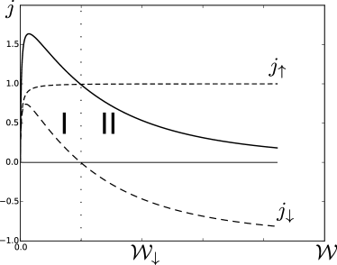
Figure 3: Dependence of photocurrent (solid line) and currents of spin-up/spin-down electrons (dashed lines) on light intensity if the initial Fermi level is below the Dirac point. The currents of each branch are proportional to the corresponding quasi-Fermi level shift. For the region I ($\mathcal{W}<\mathcal{W}_{\downarrow}/2$) edge branches contribute to net current with the same sign, while in the region II ($\mathcal{W}>\mathcal{W}_{\downarrow}/2$) the current of spin-down electrons changes its sign. Currents are measured in the units of $G_{0}\Delta\omega$.

An important limiting case is when one can neglect spin relaxation of the edge electrons assuming that $\tau_{e}\gg\tau_{C}$ and both times are great enough. In this case equation 14–15 yield $\zeta_{s}=\zeta_{-s}=-\frac{\nu_{e}}{\nu_{C}}\frac{\mu_{\uparrow}+\mu_{\downarrow}}{2}$, and the equation (13) can be solved analytically.

$$\mu_{0}=\frac{\mu_{\uparrow}+\mu_{\downarrow}}{2}=\frac{\mathcal{W}^{2}-\sqrt{\mathcal{W}^{4}+2\mathcal{W}^{2}\left(\mathcal{W}_{\uparrow}^{2}+\mathcal{W}^{2}_{\downarrow}\right)}}{(\mathcal{W}_{\uparrow}^{2}+\mathcal{W}_{\downarrow}^{2})}\Delta\omega$$ (16)

$$\delta\mu=\frac{\mathcal{W}_{\uparrow}^{2}-\mathcal{W}^{2}_{\downarrow}}{\Delta\omega\mathcal{W}^{2}}\mu_{0}^{2}$$ (17)

An electric current $j=G_{0}\delta\mu$ arises in the edge state, where $G_{0}=e^{2}/h$ is the conductance quantum. If the intensity of light is small $\mathcal{W}\ll\mathcal{W}_{\uparrow},\mathcal{W}_{\downarrow}$ (Fig 2b), mainly the spin-up electrons are excited by the light. The spin relaxation time for the bulk states is much shorter than the life-time of photogenerated electrons, hence, spin of the photogenerated electrons relaxes, and there appear additional spin-down electrons in the conduction band, whose recombination rate turns out to be greater than the excitation rate of spin-down edge electrons. Thus, the quasi Fermi level for spin-up electrons is below $\varepsilon_{F}$, and the quasi Fermi level for spin-down electrons is above it. The currents of electrons with the opposite spin contribute to the total electric current with the same sign (see Fig 3a, Fig 3c), and the total current $j\approx 2G_{0}\frac{W_{\uparrow}^{2}-W_{\downarrow}^{2}}{W_{\uparrow}^{2}+W_{\downarrow}^{2}}\Delta\omega$.

If the intensity of light $\mathcal{W}\gg\mathcal{W}_{\uparrow},\mathcal{W}_{\downarrow}$ (Fig. 3b), all the edge electrons with energies from $|\mathcal{M}|-\omega_{0}$ to $\varepsilon_{F}$ are excited to the conduction band, and the quasi Fermi levels of the edge electrons saturate at the value $\mu_{s}=-\Delta\omega$. The currents $j_{s}=G_{0}\mu_{s}$ are almost equal, but contribute to the total current with opposite signs. Thus, the total current decreases with the increase of the intensity as $j\propto\mathcal{W}^{-2}$. For an HgTe/CdTe quantum well with width $d_{c}=7\;\mathrm{nm}$, and the sample size of order $L\sim 1\;\mathrm{\mu m}$, the quasi Fermi level for spin-up electrons saturates at $\mathcal{W}\sim\mathcal{W}_{\uparrow}\sim 10^{-9}\;\mathrm{W/cm^{2}}$. The quasi Fermi level for spin-down electrons saturates at $\mathcal{W}_{\downarrow}\sim 10^{-8}\;\mathrm{W/cm^{2}}$

However, in case of extremely weak intensities spin relaxation rate turns out to be comparable with transitions rates and hence cannot be neglected. We can solve (13)–(15) analytically assuming $\mathcal{W}<\mathcal{W}_{\uparrow}\ll\mathcal{W}_{\downarrow}$ and obtain

$$j=G_{0}\Delta\omega\frac{\mathcal{W}^{2}}{4\mathcal{W}_{\uparrow}^{2}}\frac{\tau_{e}^{2}}{\tau_{C}^{2}}\left(1-\sqrt{1+16\frac{\mathcal{W}_{\uparrow}^{2}}{\mathcal{W}^{2}}\frac{\tau_{c}^{2}}{\tau_{e}^{2}}}\right)$$

The full curve for the dependence of photocurrent on intensity is sketched on the Fig. 3.

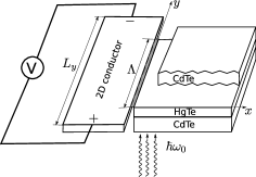
Figure 4: A proposal to detect photocurrent in the edge state: 2D conductor of length $L_{y}$ is coupled to the edge state via the tunnel contact of length $\Lambda$. The EMF appears between the opposite ends of the 2D conductor.

III Tunnel contact to an external circuit

In the previous section we showed that circularly polarized illumination induces an electric current at the edge of HgTe/CdTe quantum well TI. In order to observe the effect one should connect the sample to an external circuit. We consider a system of HgTe/CdTe tunnel-coupled by a contact of length $\Lambda$ to a 2D metal conductor (see Fig. 4).

The Hamiltonian of the system reads

$$\hat{H}=\hat{H}_{TI}+\hat{H}_{2D}+\hat{H}_{tun}$$ (18)

In order to describe the edge state we use an effective edge state Hamiltonian corresponding to the linear edge state spectrum

$$\hat{H}_{TI}=\sum\limits_{s}\int\hat{\psi}_{s}^{\dagger}(y)(-iv_{TI}s\partial_{y}+\varepsilon_{D})\hat{\psi}_{s}(y)dy,$$ (19)

where $\hat{\psi}$ is the effective field operator for an electron in the edge states, $\varepsilon_{D}$ is the energy of Dirac point measured from the middle of the band gap, $v_{TI}$ is the velocity of edge electrons. We assume that illumination results in quasi-equilibrium occupation numbers of electrons corresponding to the quasi Fermi levels, and the tunnel coupling is weak that it does not affect the optical transitions, so the results of the previous section are applicable. The Hamiltonian of the 2D conductor reads

$$\hat{H}_{2D}=\hat{H}_{2D,0}+\sum\limits_{s}\int d^{2}\mathbf{r}\;\hat{\Psi}_{s}^{\dagger}V_{imp}(\mathbf{r})\hat{\Psi}_{s},$$ (20)

where $\hat{H}_{2D,0}$ is the Hamiltonian of free 2D electrons, $\hat{\Psi}$ is the field operator in the 2D conductor. Here we take into account a random delta-correlated potential of impurities $V_{imp}$ characterized by a mean scattering time $\tau_{imp}$.

The tunneling Hamiltonian reads:

$$\hat{H}_{tun}=\sum\limits_{s}\int dy\;\hat{\psi}_{s}^{\dagger}(y)\mathcal{T}\hat{\Psi}_{s}(x=0,y)+H.c.$$ (21)

where $\mathcal{T}$ is a matrix element of tunneling, and we assume that the tunneling is momentum-conserving.

We start from the Hamiltonian (18)–(21), and then derive equations for Keldysh Green functions $G^{R(A),K}$ taking into account the tunneling Hamiltonian and the impurity potential as perturbations. The self energy of 2D electrons in the conductor resulting form the tunneling reads

$$\Sigma^{R(A),K}_{tun}(\mathbf{r}_{1},\mathbf{r}_{2})=|\mathcal{T}|^{2}\delta(x_{1})\delta(x_{2})G_{TI}^{R(A),K}(y_{1}-y_{2})$$

The Green functions of the electrons in the edge state electrons can be obtained by solving the corresponding Dyson equations:

$$G_{TI,s}^{R(A)}(\varepsilon,p_{y}) =\;\left(\varepsilon-\varepsilon_{p_{y},s}+i\Gamma\right)^{-1}$$ (22)

$$G_{TI,s}^{K}(\varepsilon,p_{y}) =\;-2\pi i\delta_{\Gamma}(\varepsilon-\varepsilon_{p_{y},s})\tanh\frac{\varepsilon-\varepsilon_{F}^{(TI)}-\mu_{s}}{2T}$$ (23)

where $\Gamma$ is the inverse life-time of electrons in the edge state, which consists of contributions from tunneling and optical transitions. The contribution from the optical transitions is determined by self energy operator $i\Gamma=\sum_{k_{y}}(\Sigma^{R}-\Sigma^{A})$ (see (67), (69)). Besides, some mechanisms of spin-relaxations, e.g. coupling to multiple puddlesVäyrynen et al. (2014) also contribute to $\Gamma$, so here we introduce it phenomenologically. Note, that the exact value of $\Gamma$ does not affect the final results. The Lorenz-type factor $\delta_{\Gamma}(x)=\frac{1}{\pi}\frac{\Gamma}{x^{2}+\Gamma^{2}}$ describes broadening of electronic states due to their finite life-time.

The derivation of kinetic equation for quasi-classical distribution function $f_{s}(\mathbf{r},\mathbf{p})$ in the 2D conductor is straightforward Keldysh (1965) and gives

$$\left[\partial_{t}+(\mathbf{v},\nabla)\right]f_{s}+\\ 2\pi|\mathcal{T}|^{2}\delta(x)\theta\left(\frac{\Lambda}{2}-|y|\right)\delta_{\Gamma}\left(\varepsilon_{p_{y},s}-\varepsilon^{(2D)}_{\mathbf{p},s}\right)\left[f_{s}-n_{s}\right]=\\ \frac{\bar{f}_{s}-f_{s}}{\tau}$$ (24)

Here $n_{s}$ is a distribution function for the edge state electrons the TI, and the Heaviside step-function $\theta$ restricts the length of the contact to $\Lambda$.

If the TI is illuminated by circular-polarized light, the quasi Fermi level of spin-up electrons is lower than the quasi Fermi level of spin-down electrons. In a stationary regime the current through the tunnel contact should be equal to zero, therefore, the Fermi level in the 2D conductor is exactly in the middle between the quasi Fermi levels in the edge states of TI. However, the zero tunnel current consists of a spin-up current from the TI to the conductor and a spin-down current from the conductor to TI. Electrons of the opposite spins in the TI are of the opposite chiralities and the tunneling is assumed to conserve momentum,so it should result in an electron drift and appearance of the counterbalancing EMF in the conductor. We consider a stationary case in which tunneling leads to charge redistribution, and, hence, the extra charge induces an electric field.The electric field $\mathbf{E}$ is related with the extra charge $-|e|\delta\rho$ by the Poisson equation:

$$\mathrm{div}\;\mathbf{E}=-4\pi|e|\delta\rho,$$ (25)

where $\delta\rho$ is the deviation of electron density from its equilibrium value, and the full electron density can be expressed in terms of the distribution function as

$$\rho=\sum\limits_{s}\int\frac{d^{2}\mathbf{p}}{(2\pi)^{2}}\bar{f}_{s}$$ (26)

The kinetic equation that takes into account the electric field in the conductor reads

$$\left[\partial_{t}+(\mathbf{v},\nabla)\right]f_{s}+\Pi_{s}+\frac{f_{s}-\bar{f}_{s}}{\tau}-|e|\mathbf{v}\mathbf{E}\frac{\partial f_{s}}{\partial\varepsilon}=0,$$ (27)

$$\Pi_{s}=\theta\left(\frac{\Lambda}{2}-|y|\right)2\pi|\mathcal{T}|^{2}\delta(x)\delta_{\Gamma}\left(\varepsilon_{p_{y},s}-\varepsilon^{(2D)}_{\mathbf{p},s}\right)\left[f_{s}-n_{s}\right]$$ (28)

Here $\Pi_{s}$ denotes the term responsible for the tunneling. Since the electric field $\mathbf{E}$ arises due to the deviation of the distribution function $f$ from its equilibrium unperturbed value $f_{0}$, we can replace $f_{s}$ in the field term with $f_{0}$, neglecting second-order corrections.

We consider a model where the 2D conductor is a narrow strip spanning from $x=-L_{x}/2$ and $x=L_{x}/2$ and is infinite in $y$-direction, and the contact is in the middle of the strip at $x=0$. For simplicity we assume that the width $L_{x}$ of the conductor is smaller than the scattering length $v_{F}\tau$. In a more general case the conductor can be qualitatively considered as the same narrow strip with a bypass resistance. Under these assumptions one can take into account only the electric field along the contact $E_{y}\gg E_{x}$.

We solve the kinetic equation together with the Poisson equation assuming quasi-neutrality and treating the angle-averaged distribution function $\bar{f}_{s}$ in the impurity term self-consistently (for details see Appendix E).

Finally, we obtain the EMF as the integral over the conductor length of the electric field averaged in the transversal direction $\langle E_{y}\rangle_{x}=L_{x}^{-1}\int\limits_{-L_{x}/2}^{L_{x}/2}E_{y}\;dx$:

$$|e|\mathcal{E}=\int\limits_{-L_{y}/2}^{L_{y}/2}|e|\langle E_{y}\rangle_{x}\;dy=\\ -\frac{|\mathcal{T}|^{2}}{v_{F}}\frac{2(\varepsilon_{F}^{(TI)}-\varepsilon_{D})}{\sqrt{\left(p_{F}v_{TI}\right)^{2}-(\varepsilon_{F}^{(TI)}-\varepsilon_{D})^{2}}}\frac{\Lambda}{L_{x}}\frac{\delta\mu}{v_{TI}p_{F}},$$ (29)

where $p_{F}$, $v_{F}$ are the Fermi momentum and velocity in the conductor, and $\delta\mu$ is the difference between quasi Fermi levels given by (17)

IV Conclusions

In summary, we considered electric dipole optical transitions from helical edge states of HgTe/CdTe TI illuminated by circularly polarized light to the bulk conduction band. If electron-hole symmetry is broken which typically is the case, these optical transitions are strongly spin-dependent.

This gives rise to a circular electric current in the edge state if the Fermi level is below the Dirac point. The value of the photocurrent reaches maximum and then decreases with the growth of the light intensity. It is worth noting that although the overlap between wavefunctions of the edge and bulk states determines the time required for stationary regime to settle in, the magnitude of the current in this regime does not depend on the overlap, and, hence, we anticipate that the effect can be observed even in samples where this overlap is small. We showed that the photocurrent can be detected electrically by measuring EMF in the conductor coupled to the edge state of the TI.

Appendix A Optical transitions in the case of electron-hole symmetry

In this section the matrix elements of the optical transitions are explicitly calculated for the case of electron-hole symmetry $\mathcal{D}=0$. In this case, the Hamiltonian (1) with zero boundary conditions yields the edge state wavefunction

$$\psi_{edge,s}(x,k_{y})=\Psi_{edge,s}\left(e^{-\lambda_{s,-}x}-e^{-\lambda_{s,+}x}\right),$$

$$\Psi_{edge,\uparrow}\propto\begin{pmatrix}i\\ 1\\ 0\\ 0\end{pmatrix},\quad\Psi_{edge,\downarrow}\propto\begin{pmatrix}0\\ 0\\ -i\\ 1\\ \end{pmatrix},$$ (30)

where $\lambda_{+}\approx\frac{\mathcal{A}}{|\mathcal{B}|}$, $\lambda_{-}\approx\frac{|\mathcal{M}|}{\mathcal{A}}\ll\lambda_{+}$. Here we assumed that $\mathcal{A}^{2}\gg\mathcal{B}\mathcal{M}$, which is the case for the typical parameters of TI. Solving Schroedinger equation with zero boundary condition for $\epsilon-|M|\ll|M|$, $k_{y}=0$ we obtain bulk wavefunctions near the bottom of the conduction band:

$$\psi_{bulk,\uparrow}(\epsilon)\propto\begin{pmatrix}\cos k_{x}x+\frac{k_{x}\mathcal{A}}{2\mathcal{M}}\sin k_{x}x\\ i\cos k_{x}x-\frac{2i\mathcal{M}}{k_{x}\mathcal{A}}\sin k_{x}x\\ 0\\ 0\end{pmatrix}-\begin{pmatrix}1\\ i\\ 0\\ 0\end{pmatrix}e^{-\kappa x},$$ (31)

$$\psi_{bulk,\downarrow}(\epsilon)\propto\begin{pmatrix}0\\ 0\\ \cos k_{x}x+\frac{k_{x}\mathcal{A}}{2\mathcal{M}}\sin k_{x}x\\ -i\cos k_{x}x+\frac{2i\mathcal{M}}{k_{x}\mathcal{A}}\sin k_{x}x\end{pmatrix}-\begin{pmatrix}0\\ 0\\ 1\\ -i\end{pmatrix}e^{-\kappa x},$$ (32)

where $k_{x}\approx\frac{\sqrt{\epsilon^{2}-\mathcal{M}^{2}}}{\mathcal{A}}\ll\lambda_{-}$ and $\kappa\approx\frac{\mathcal{A}}{|\mathcal{B}|}\approx\lambda_{+}$. The first terms in (31)–(32) correspond to the superposition of incident and reflected waves, while the second terms correspond to the parts of wavefunctions localized near the boundary. In the presence of the boundary the angular momentum is ill-defined. Although the wavefunctions of the conduction band behave like $|H_{1},m_{j}=3/2\rangle$ and $|H_{1},m_{j}=-3/2\rangle$ with a well-defined angular momentum far away from the boundary at $x\gg k_{x}^{-1}$, the overlap integral between edge and bulk states is dominated by small distances from the boundary $x\sim\lambda_{-}^{-1}$, where these wavefunctions are superpositions of $|E_{1}\rangle$, $|H_{1}\rangle$ with equal (up to a phase factor) amplitudes:

$$\psi_{bulk,\uparrow}(\epsilon)\sim\begin{pmatrix}1\\ i\\ 0\\ 0\end{pmatrix}\left(1-e^{-\kappa x}\right),$$ (33)

$$\psi_{bulk,\downarrow}(\epsilon)\sim\begin{pmatrix}0\\ 0\\ 1\\ -i\end{pmatrix}\left(1-e^{-\kappa x}\right),$$ (34)

Thus, the matrix elements are equal up to a phase factor $|w_{\uparrow}|^{2}=|w_{\downarrow}|^{2}\sim\frac{1}{L_{x}\lambda_{-}^{3}}$.

Appendix B Optical transitions in the case of strong electron-hole asymmetry

In this section we analytically derive matrix elements of the optical transitions in the case of strong electron-hole asymmetry, i.e. $|\mathcal{B}-\mathcal{D}|\ll\mathcal{B}$. For the simplicity we consider transitions between the Dirac point $k_{y}=0$ and the bottom of the conduction band $\varepsilon-|\mathcal{M}|\ll|\mathcal{M}|\sqrt{\mathcal{B}^{2}-\mathcal{D}^{2}}/B$. We also assume that typically $\mathcal{A}^{2}\gg\mathcal{B}\mathcal{M}$. For the edge states we can use the expression (5), where $\lambda_{-}\approx\frac{|\mathcal{M}|\sqrt{\mathcal{B}^{2}-\mathcal{D}^{2}}}{2\mathcal{A}\mathcal{B}}$, $\lambda_{+}\approx\frac{\mathcal{A}}{\sqrt{\mathcal{B}^{2}-\mathcal{D}^{2}}}\gg\lambda_{-}$.

The bulk eigen-state of Hamiltonian 1 for energy $\varepsilon>|\mathcal{M}|$ is a sum of a right-moving wave, a left-moving wave and a term localized in the vicinity of the boundary:

$$\psi^{(bulk)}_{s,k_{y}} \propto\psi^{L}+t_{R}\psi^{R}+t_{d}\psi^{d}$$ (35)

$$\psi^{L} =e^{-ik_{x}x}\left(-\frac{Ask_{x}}{M}\left|E_{1},s\right\rangle+\left|H_{1},s\right\rangle\right)$$ (36)

$$\psi^{R} =e^{ik_{x}x}\left(\frac{Ask_{x}}{M}\left|E_{1},s\right\rangle+\left|H_{1},s\right\rangle\right)$$ (37)

$$\psi^{d} =e^{-\kappa x}\left(\frac{iAs}{B\kappa}\left|E_{1},s\right\rangle+\left|H_{1},s\right\rangle\right),$$ (38)

where $\kappa\approx\lambda_{+}$, $k_{x}=\frac{\sqrt{\varepsilon^{2}-\mathcal{M}^{2}}}{\mathcal{A}}\ll\kappa,\lambda_{-}$. Amplitudes $t_{R}$ and $t_{d}$ can be obtained using the zero-boundary condition $\psi^{(bulk)}(x=0)=0$. It yields

$$t_{R}=\frac{\mathcal{B}k_{x}\kappa+i\mathcal{M}}{\mathcal{B}k_{x}\kappa-i\mathcal{M}}\approx-1,\quad t_{d}=-\frac{2\mathcal{B}k_{x}\kappa}{\mathcal{B}k_{x}\kappa-i\mathcal{M}}\approx-2\frac{\mathcal{B}ik_{x}\kappa}{\mathcal{M}}$$ (39)

Now the matrix elements can be calculated straightforwardly. First, we find the overlap integrals defined in the section II:

$$F=-\frac{2ik_{x}}{\lambda_{-}^{2}}\frac{1}{\sqrt{2L_{x}}},\quad G=-\frac{2\mathcal{A}k_{x}}{\mathcal{M}\lambda_{-}}\frac{1}{\sqrt{2L_{x}}}$$ (40)

The matrix elements of the transitions can be calculated as

$$|w_{\uparrow}|^{2}=|G|^{2}\frac{|\mathcal{B}-\mathcal{D}|}{4|\mathcal{B}|\lambda_{-}}=\frac{\mathcal{A}^{2}k_{x}^{2}}{2|\mathcal{M}|^{2}\lambda_{-}^{3}L_{x}}\frac{|\mathcal{B}-\mathcal{D}|}{|\mathcal{B}|}$$ (41)

$$|w_{\downarrow}|^{2}=|F|^{2}\frac{1}{2\lambda_{-}}=\frac{2k_{x}^{2}}{\lambda_{-}^{5}L_{x}}$$ (42)

Appendix C Matrix elements for the light incident at an arbitrary angle

In this section we derive the matrix elements (8) for light incident in the direction $\mathbf{n}^{\theta,\phi}$. We can take an auxiliary orthonormal basis

$$\mathbf{e}_{x}^{\theta,\phi} =\mathbf{e}_{x}\cos\phi\cos\theta+\mathbf{e}_{y}\sin\phi\cos\theta-\mathbf{e}_{z}\sin\theta$$ (43)

$$\mathbf{e}_{y}^{\theta,\phi} =-\mathbf{e}_{x}\sin\phi+\mathbf{e}_{y}\cos\phi$$ (44)

$$\mathbf{e}_{z}^{\theta,\phi} =\mathbf{n}^{\theta,\phi}=\mathbf{e}_{x}\cos\phi\sin\theta+\mathbf{e}_{y}\sin\phi\sin\theta+\mathbf{e}_{z}\cos\theta$$ (45)

The vector potential reads

$$\mathbf{A}^{\theta,\phi}=\mathbf{e}_{x}^{\theta,\phi}A_{0}\cos\omega_{0}t-\mathbf{e}_{y}^{\theta,\phi}A_{0}\sin\omega_{0}t$$ (46)

$$A_{x}^{\theta,\phi}=A_{0}\left(\cos\phi\cos\theta\cos\omega_{0}t+\sin\phi\sin\omega_{0}t\right)$$ (47)

$$A_{y}^{\theta,\phi}=A_{0}\left(\sin\phi\cos\theta\cos\omega_{0}t-\cos\phi\sin\omega_{0}t\right)$$ (48)

$$A_{z}^{\theta,\phi}=-A_{0}\sin\theta\cos\omega_{0}t$$ (49)

where the amplitude $A_{0}=\frac{\sqrt{4\pi\mathcal{W}}}{n_{r}\omega_{0}}$ (cf. Eq. 4). Since only in-plane components of the vector potential yield the optical transitions, the case of arbitrary direction of light is equivalent to the case of elliptical polarization with $\sin\theta$ standing for the eccentricity.

The light-matter interaction Hamiltonian (2) can be now rewritten as

$$\hat{H}_{e-A}^{\theta,\phi}=\frac{A_{0}}{2}e^{i\omega_{0}t}\left[\hat{H}_{1}e^{-i\varphi}(\cos\theta+1)+\right.\\ \left.\hat{H}_{1}^{\dagger}e^{i\varphi}(\cos\theta-1)\right]+H.c.$$ (50)

Time-reversal symmetry allows us to relate the matrix elements of $\hat{H}_{1}$ and $\hat{H}_{1}^{\dagger}$

$$\left\langle\psi_{edge,s}\middle|\hat{H}_{1}^{\dagger}\middle|\psi_{bulk,s}\right\rangle=-\left\langle\psi_{edge,-s}\middle|\hat{H}_{1}\middle|\psi_{bulk,-s}\right\rangle^{*}$$ (51)

This imply the relation between the matrix elements for different directions of the light

$$w_{s}^{\theta,\phi}=\frac{w_{s}e^{-i\phi}(\cos\theta+1)+w_{-s}^{*}e^{i\phi}(1-\cos\theta)}{2}$$ (52)

Appendix D Derivation of kinetic equation

In order to derive kinetic equation it is convenient to write a second-quantized Hamiltonian by expanding the field operator in eigen basis of $\hat{H}_{BHZ}$: $\hat{\psi}=\sum\limits_{k_{y}}\hat{a}_{k_{y}}\psi^{(e)}_{k_{y}}+\sum\limits_{k_{x},k_{y}}\left[\hat{c}_{k_{x},k_{y}}\psi^{(c)}_{k_{x}}+\hat{v}_{k_{x},k_{y}}\psi^{(v)}_{k_{x}}\right]$, where $\psi^{(e)}$ is the $4\times 1$ wavefunction of the edge mode, $\psi^{(c)}$, $\psi^{(v)}$ are $4\times 1$ wavefunctions in conduction and valence bands correspondingly. In this basis the Hamiltonian reads

$$\begin{split}\hat{H}_{BHZ}&=\;\sum\limits_{s,k_{y}}\varepsilon_{s,k_{y}}\hat{a}_{s,k_{y}}^{\dagger}\hat{a}_{s,k_{y}}+\sum\limits_{s,k_{x},k_{y}}\epsilon^{(c)}_{k_{x},k_{y}}\hat{c}_{s,k_{y}}^{\dagger}\hat{c}_{s,k_{y}}+\\ &\sum\limits_{s,k_{x},k_{y}}\epsilon^{(v)}_{k_{x},k_{y}}\hat{v}_{s,k_{x},k_{y}}^{\dagger}\hat{v}_{s,k_{x},k_{y}},\end{split}$$ (53)

$$\begin{split}\hat{H}_{e-A}&=\sum\limits_{s,k_{x},k_{y}}\left[w_{s}(\hat{{A}}_{x}-i\hat{{A}}_{y})+\right.\\ &\left.w_{-s}(\hat{{A}}_{x}+i\hat{{A}}_{y})\right]\hat{a}_{s,k_{y}}^{{\dagger}}\hat{c}_{s,k_{x},k_{y}}+H.c.\end{split}$$ (54)

where $\epsilon^{(c)}_{k_{x},k_{y}}$, $\epsilon^{(v)}_{k_{x},k_{y}}$ are the energies in the conduction and valence bands correspondingly. Here we disregard transitions between the edge states and the valence band as the frequency of illumination $\omega_{0}$ is assumed to be much smaller than the difference between the Fermi level and the top of the valence band.

The correlations of quantum fluctuations $\delta\hat{\mathbf{A}}$ are given by the Green’s functions $D^{R}_{\alpha\beta}(1,1^{\prime})=-i\theta(t-t^{\prime})\left\langle\left[\delta\hat{{A}}_{\alpha}(1),\delta\hat{{A}}_{\beta}(1^{\prime})\right]\right\rangle$, $D^{A}_{\alpha\beta}(1,1^{\prime})=i\theta(t^{\prime}-t)\left\langle\left[\delta\hat{{A}}_{\alpha}(1),\delta\hat{{A}}_{\beta}(1^{\prime})\right]\right\rangle$, $D^{K}=-i\left\langle\left\{\delta\hat{{A}}_{\alpha}(1),\delta\hat{{A}}_{\beta}(1^{\prime})\right\}\right\rangle$. At zero temperature these Green’s functions are of the form

$$D^{R(A)}_{\alpha\beta}(\omega,k) =\;\frac{4\pi}{(n_{r}\omega)^{2}}\frac{(n_{r}\omega)^{2}\delta_{\alpha\beta}-k_{\alpha}k_{\beta}}{\epsilon\omega^{2}-|k|^{2}\pm i0},$$ (55)

$$\quad D^{K} =\;(D^{R}-D^{A})\mathrm{sign}\;\omega$$ (56)

However, due to the form of the Hamiltonian (54) it is convenient to introduce axillary scalar fields

$$\hat{\tilde{A}}_{s}=w_{s}(\hat{{A}}_{x}-i\hat{{A}}_{y})+w_{-s}(\hat{{A}}_{x}+i\hat{{A}}_{y}).$$

Then the Green’s function for these fields $\tilde{D}^{R}_{s}(1,1^{\prime})=-i\theta(t-t^{\prime})\left\langle\left[\delta\hat{{\tilde{A}}}_{s}(1),\delta\hat{\tilde{A}}^{\dagger}_{s}(1^{\prime})\right]\right\rangle$, $\tilde{D}^{A}_{s}(1,1^{\prime})=i\theta(t^{\prime}-t)\left\langle\left[\delta\hat{\tilde{A}}_{s}(1),\delta\hat{{\tilde{A}}}^{\dagger}_{s}(1^{\prime})\right]\right\rangle$, $\tilde{D}^{K}_{s}=-i\left\langle\left\{\delta\hat{{\tilde{A}}}_{s}(1),\delta\hat{{\tilde{A}}}_{\beta}(1^{\prime})\right\}\right\rangle$ take up the form

$$\tilde{D}^{R(A,K)}_{s}=D_{xx}|w_{s}+w_{-s}|^{2}+D_{yy}|w_{s}-w_{-s}|^{2}-\\ i(D_{xy}+D_{yx})(w_{s}w_{-s}^{*}-w_{-s}w_{s}^{*})$$ (57)

We treat the interaction between electromagnetic field $\hat{\mathcal{A}}$ and electrons given by (54) as a perturbation, and use the Keldysh perturbation theory in order to derive the retarded, advanced and Keldysh Green’s functions $G^{R,A,K}_{edge}$ of electrons in the edge states. The Dyson equations reads

$$\begin{split}&(i\partial_{t}-\varepsilon_{s,k_{y}})G^{R(A)}_{edge,s}(t,t^{\prime})-\int dt^{\prime\prime}\Sigma^{R(A)}_{s}(t,t^{\prime\prime})G^{R(A)}_{edge,s}(t^{\prime\prime},t^{\prime})=\\ &\delta(t-t^{\prime})\end{split}$$ (58)

$$\begin{split}&(i\partial_{t}-\varepsilon_{s,k_{y}})G^{K}_{edge,s}(t,t^{\prime})-\\ &\int dt^{\prime\prime}\left[\Sigma^{R}_{s}(t,t^{\prime\prime})G^{K}_{edge,s}(t^{\prime\prime},t^{\prime})+\Sigma^{K}_{s}(t,t^{\prime\prime})G^{A}_{edge,s}(t^{\prime\prime},t^{\prime})\right]=0\end{split}$$ (59)

$$\begin{split}&\left(-i\partial_{t^{\prime}}-\varepsilon_{s,k_{y}}\right)G^{K}_{edge,s}(t,t^{\prime})-\\ &\int dt^{\prime\prime}\left[G^{R}_{edge,s}(t,t^{\prime\prime})\Sigma^{K}_{s}(t^{\prime\prime},t^{\prime})+G^{K}_{edge,s}(t,t^{\prime\prime})\Sigma^{A}_{s}(t^{\prime\prime},t^{\prime})\right]=0\end{split}$$ (60)

The self-energy $\Sigma$ can be represented as the sum of a classical contribution $\Sigma_{ind}$ a contribution $\Sigma_{sp}$ due to quantum fluctuations $\delta\hat{\mathcal{A}}$, which is responsible for spontaneous transitions

$$\Sigma=\;\Sigma_{ind}+\Sigma_{sp},$$ (61)

$$\Sigma^{R(A,K)}_{ind,s}=\;\sum\limits_{s,k_{x}}\langle\tilde{\mathcal{A}_{s}}(t)\rangle G^{R(A,K)}_{c,s}(k_{x},t,t^{\prime})\langle\tilde{\mathcal{A}_{s}^{*}}(t^{\prime})\rangle,$$ (62)

$$\Sigma_{sp,s}^{R}(t-t^{\prime},y-y^{\prime})=\;\frac{i}{2}\left(\tilde{D}^{R}_{s}G^{K}_{c,s}+\tilde{D}^{K}_{s}G^{R}_{c,s}\right)$$ (63)

$$\Sigma_{sp,s}^{K}(t-t^{\prime},y-y^{\prime})=\;\frac{i}{2}\left(\tilde{D}^{K}_{s}G^{K}_{c,s}+\tilde{D}^{R}_{s}G^{R}_{c,s}+\tilde{D}^{A}_{s}G^{A}_{c,s}\right)$$ (64)

Since the classical value of electromagnetic field $\langle\mathbf{A}\rangle$ depends on time the self-energy $\Sigma_{ind}$ depend both on the sum of the times $t_{s}=t+t^{\prime}$ and their difference $t_{a}=t-t^{\prime}$. However, the dependence on the sum of the times describes the motion of electrons in high-frequency electromagnetic field, and we disregard it leaving only the dependence on the time difference, which is responsible for induced transitions. After performing the Fourier transform over the difference time we obtain

$$\Sigma_{ind,s}^{R(A,K)}(\varepsilon,k_{y})=\frac{4\pi\mathcal{W}}{(n_{r}\omega_{0})^{2}}\sum\limits_{k_{x}}|w_{s}|^{2}G^{R(A,K)}_{c,s}(\varepsilon+\omega_{0},k_{y})+\\ |w_{-s}|^{2}G^{R(A,K)}_{c,s}(\varepsilon-\omega_{0},k_{y})$$ (65)

The kinetic equation for the distribution function $n_{s}(\varepsilon)$ of electrons in the edge state may be derived in the standard way by subtracting the Dyson equations with self-energy operators acting from the left (59) and from the right (60), integrating over $k_{y}$, and using the relation $G^{K}=\left(G^{R}-G^{A}\right)\left[1-2n_{s}(\varepsilon)\right]$:

$$2\partial_{t}n(\varepsilon)=i\left[1-2n(\varepsilon)\right]\left(\Sigma^{R}(k_{y})-\Sigma^{A}(k_{y})\right)-i\Sigma^{K}(k_{y})$$ (66)

Using Eqs. (63) –(65) and the expression for the Green’s functions in the conduction band $G^{R(A)}_{c,s}=1/\left(\varepsilon-\epsilon_{k_{x},k_{y}}\pm i0\right)$, $G^{K}=\left(G^{R}-G^{A}\middle)\middle[1-2N_{s}\right]$, where $N_{s}(\varepsilon)$ is the distribution function of electrons in the conduction band, the summation over $k_{x}$ in the self-energy operators is straightforward:

$$\Sigma^{R}_{ind}(\varepsilon,k_{y})-\Sigma^{A}_{ind}(\varepsilon,k_{y})=\;-2\pi i\frac{4\pi\mathcal{W}}{(n_{r}\omega_{0})^{2}}|w_{s}|^{2}\tilde{\nu}_{c,k_{y}}(\varepsilon+\omega_{0})$$ (67)

$$\begin{split}&\Sigma^{K}_{ind}(\varepsilon,k_{y})=\;\\ &-2\pi i\frac{4\pi\mathcal{W}}{(n_{r}\omega_{0})^{2}}|w_{s}|^{2}\tilde{\nu}_{c,k_{y}}(\varepsilon+\omega_{0})\left[1-2N_{s}(\varepsilon+\omega_{0})\right]\end{split}$$ (68)

$$\begin{split}&\Sigma^{R}_{sp}(\varepsilon,k_{y})-\Sigma^{A}_{sp}(\varepsilon,k_{y})=\;\\ &-\frac{8i}{3}\int\left(|w_{s}|^{2}+|w_{-s}|^{2}\right)\tilde{\nu}_{c,k_{y}}(\varepsilon+\omega)\;N(\varepsilon+\omega)\omega n_{r}\;d\omega\end{split}$$ (69)

$$\begin{split}&\Sigma^{K}_{sp}(\varepsilon,k_{y})=\\ &-\frac{8i}{3}\int\left(|w_{s}|^{2}+|w_{-s}|^{2}\right)\tilde{\nu}_{c,k_{y}}(\varepsilon+\omega)\;N(\varepsilon+\omega)\omega n_{r}\;d\omega\end{split}$$ (70)

The final kinetic equation can be obtained by substituting the self-energy operators into (66):

$$\begin{split}\frac{dn_{s}(\varepsilon)}{dt}&=\;-\frac{n_{s}(\varepsilon)-N_{s}(\varepsilon+\omega_{0})}{\tau_{ind,s}(\varepsilon,\varepsilon+\omega_{0})}\mathcal{W}+\\ &\int\frac{N_{s}(\varepsilon+\omega)\left[1-n_{s}(\varepsilon)\right]}{\tau_{sp}(\varepsilon+\omega,\varepsilon)}d\omega\end{split}$$ (71)

$$\tau_{ind,s}^{-1} =\;8\pi^{2}\tilde{\nu}_{C,k_{y}}(\varepsilon+\omega_{0})\frac{|w_{s}|^{2}}{n_{r}^{2}\omega_{0}^{2}},$$ (72)

$$\tau_{sp}^{-1} =\;\frac{8}{3}\left(|w_{s}|^{2}+|w_{-s}|^{2}\right)\omega\tilde{\nu}_{C,k_{y}}(\varepsilon+\omega)n_{r}$$ (73)

Appendix E EMF calculation

From the kinetic equation (27), one can express the distribution function $f_{s}$ and its angle-averaged value $\left\langle f_{s}\right\rangle_{\varphi}$ via the tunneling source $\Pi_{s}$ defined in (28):

$$\left\langle f_{s}\right\rangle_{\varphi}=\left(\left\langle\frac{1}{i\mathbf{v}\mathbf{k}_{\parallel}+\tau^{-1}}\right\rangle_{\varphi}-\tau^{-1}\right)^{-1}\left(-\Pi_{s}+|e|\mathbf{v}\mathbf{E}\frac{\partial f_{0}}{\partial\varepsilon}\right),$$ (74)

where $\mathbf{k}=\left(\mathbf{k}_{\parallel},k_{z}\right)$ is a parameter of spatial Fourier transform.

The quasi-neutrality condition implies

$$\int\left\langle\frac{\mathbf{v}|e|\mathbf{E}\frac{\partial f_{0}}{\partial\varepsilon}}{i\mathbf{v}\mathbf{k}_{\parallel}+\tau^{-1}}\right\rangle_{\varphi}\;d\xi=\sum\limits_{s}\int\left\langle\frac{\Pi_{s}}{i\mathbf{v}\mathbf{k}_{\parallel}+\tau^{-1}}\right\rangle_{\varphi}\;d\xi$$ (75)

Using the relation $\left\langle\frac{1}{i\mathbf{v}\mathbf{k}_{\parallel}+\tau^{-1}}\right\rangle_{\varphi}=\frac{\tau}{\sqrt{1+k_{\parallel}^{2}l_{\tau}^{2}}}$, and $\left\langle\frac{\mathbf{v}\mathbf{E}}{i\mathbf{v}\mathbf{k}_{\parallel}+\tau^{-1}}\right\rangle_{\varphi}=-\frac{i\mathbf{k}_{\parallel}\mathbf{E}}{k_{\parallel}^{2}}\left(1-\frac{1}{\sqrt{1+k_{\parallel}^{2}l_{\tau}^{2}}}\right)$ we obtain the final equation for the electric field

$$|e|\mathbf{k}_{\parallel}\mathbf{E}=\frac{i}{2}\sum\limits_{s}\int\left\langle\frac{\Pi_{s}}{i\mathbf{v}\mathbf{k}_{\parallel}+\tau^{-1}}\right\rangle_{\varphi}\;d\xi\frac{k_{\parallel}^{2}\sqrt{1+k_{\parallel}^{2}l_{\tau}^{2}}}{\sqrt{1+k_{\parallel}^{2}l_{\tau}^{2}}-1}$$ (76)

The electric field averaged over the lateral direction $x$ corresponds to the $k_{x}=0$ component:

$$\left\langle E_{y}\right\rangle_{x}(y)=\\ \frac{i}{2L_{x}}\sum\limits_{s}\int\left\langle\tilde{\Pi}_{s}\frac{e^{ik_{y}y}}{ivk_{y}\cos\varphi+\tau^{-1}}\right\rangle_{\varphi}\times\\ \frac{2\sin\frac{k_{y}\Lambda}{2}\sqrt{1+k_{y}^{2}l_{\tau}^{2}}}{\sqrt{1+k_{y}^{2}l_{\tau}^{2}}-1}\;d\xi\frac{dk_{y}}{2\pi},$$ (77)

where $\tilde{\Pi}_{s}=2\pi|\mathcal{T}|^{2}\delta(x)\delta_{\Gamma}\left(\varepsilon_{p_{y},s}-\varepsilon^{(2D)}_{\mathbf{p},s}\right)\left[f_{s}-n_{s}\right]$ We perform averaging over $\varphi$, assuming that the angles with $\cos\varphi$ close to $s\frac{\varepsilon^{2D}-\varepsilon_{0}}{p_{F}v_{TI}}$ give the main contribution. After summation over spin index and integrating over $\xi=v_{F}(|p|-p_{F})$ we obtain

$$\left\langle E_{y}\right\rangle_{x}(y)=\\ \frac{\pi|\mathcal{T}|^{2}\delta\mu}{L_{x}p_{F}v_{TI}\tan\varphi_{0}}\int\frac{vk_{y}e^{ik_{y}y}}{v^{2}k_{y}^{2}\cos^{2}\varphi_{0}+\tau^{-2}}\frac{2\sin\frac{k_{y}\Lambda}{2}\sqrt{1+k_{y}^{2}l_{\tau}^{2}}}{\sqrt{1+k_{y}^{2}l_{\tau}^{2}}-1}\;\frac{dk_{y}}{2\pi}$$ (78)

The EMF can be obtained as the integral of the mean electric field $\mathcal{E}=\int\limits_{-L_{y}/2}^{L_{y}/2}\langle E_{y}\rangle_{x}\;dy$:

$$\mathcal{E}=\frac{2\pi v|\mathcal{T}|^{2}\delta\mu}{L_{x}\tan\varphi_{0}}\int\frac{\sin\frac{k_{y}L_{y}}{2}}{v^{2}k_{y}^{2}\cos^{2}\varphi_{0}+\tau^{-2}}\frac{2\sin\frac{k_{y}\Lambda}{2}\sqrt{1+k_{y}^{2}l_{\tau}^{2}}}{\sqrt{1+k_{y}^{2}l_{\tau}^{2}}-1}\;d\xi\frac{dk_{y}}{2\pi}$$ (79)

The integration can be easily performed if $L_{y},\Lambda\gg l_{\tau}$, i.e. when it is dominated by smal values of $k_{y}$

$$|e|\mathcal{E}=-\frac{|\mathcal{T}|^{2}}{v_{F}}\frac{2(\varepsilon_{F}^{(TI)}-\varepsilon_{D})}{\sqrt{\left(p_{F}v_{TI}\right)^{2}-(\varepsilon_{F}-\varepsilon_{D})^{2}}}\frac{\Lambda}{L_{x}}\frac{\delta\mu}{v_{TI}p_{F}}.$$ (80)

References

- König et al. (2008) M. König, H. Buhmann, L. W. Molenkamp, T. Hughes, C.-X. Liu, X.-L. Qi, and S.-C. Zhang, J. Phys. Soc. Jpn. 77, 031007 (2008).
- Hasan and Kane (2010) M. Z. Hasan and C. L. Kane, Rev. Mod. Phys. 82, 3045 (2010).
- Qi and Zhang (2011) X.-L. Qi and S.-C. Zhang, Reviews of Modern Physics 83, 1057 (2011).
- Muniz and Sipe (2014) R. A. Muniz and J. E. Sipe, Physical Review B 89, 205113 (2014).
- McIver et al. (2012) J. McIver, D. Hsieh, H. Steinberg, P. Jarillo-Herrero, and N. Gedik, Nature nanotechnology 7, 96 (2012).
- Misawa et al. (2011) T. Misawa, T. Yokoyama, and S. Murakami, Physical Review B 84, 165407 (2011).
- Junck et al. (2013) A. Junck, G. Refael, and F. von Oppen, Physical Review B 88, 075144 (2013).
- Hosur (2011) P. Hosur, Physical Review B 83, 035309 (2011).
- Jozwiak et al. (2013) C. Jozwiak, C.-H. Park, K. Gotlieb, C. Hwang, D.-H. Lee, S. G. Louie, J. D. Denlinger, C. R. Rotundu, R. J. Birgeneau, Z. Hussain, et al., Nature Physics 9, 293 (2013).
- Zhang et al. (2010) X. Zhang, J. Wang, and S.-C. Zhang, Physical Review B 82, 245107 (2010).
- Park and Louie (2012) C.-H. Park and S. G. Louie, Physical review letters 109, 097601 (2012).
- Wu et al. (2012) Q. S. Wu, S. N. Zhang, Z. Fang, and X. Dai, Physica E: Low-dimensional Systems and Nanostructures 44, 895 (2012).
- Zhu et al. (2014) Z.-H. Zhu, C. Veenstra, S. Zhdanovich, M. Schneider, T. Okuda, K. Miyamoto, S.-Y. Zhu, H. Namatame, M. Taniguchi, M. Haverkort, et al., Physical review letters 112, 076802 (2014).
- Li and Carbotte (2013) Z. Li and J. P. Carbotte, Phys. Rev. B 88, 045414 (2013).
- Wilson et al. (2014) J. H. Wilson, D. K. Efimkin, and V. M. Galitski, Phys. Rev. B 90, 205432 (2014).
- Bernevig et al. (2006) B. A. Bernevig, T. L. Hughes, and S.-C. Zhang, Science 314, 1757 (2006).
- Diehl et al. (2009) H. Diehl, V. A. Shalygin, L. E. Golub, S. A. Tarasenko, S. N. Danilov, V. V. Bel’kov, E. G. Novik, H. Buhmann, C. Brüne, L. W. Molenkamp, et al., Physical Review B 80, 075311 (2009).
- Wittmann et al. (2010) B. Wittmann, S. Danilov, V. Bel’kov, S. Tarasenko, E. G. Novik, H. Buhmann, C. Brüne, L. W. Molenkamp, Z. Kvon, N. Mikhailov, et al., Semiconductor Science and Technology 25, 095005 (2010).
- Scharf et al. (2015) B. Scharf, A. Matos-Abiague, I. Žutić, and J. Fabian, “Probing topological transitions in HgTe/CdTe quantum wells by magneto-optical measurements,” (2015), arXiv:1502.05605 .
- Artemenko and Kaladzhyan (2013) S. N. Artemenko and V. Kaladzhyan, JETP letters 97, 82 (2013).
- Novik et al. (2005) E. G. Novik, A. Pfeuffer-Jeschke, T. Jungwirth, V. Latussek, C. R. Becker, G. Landwehr, H. Buhmann, and L. W. Molenkamp, Physical Review B 72, 035321 (2005).
- Zhang et al. (2009) H. Zhang, C.-X. Liu, X.-L. Qi, X. Dai, Z. Fang, and S.-C. Zhang, Nature Physics 5, 438 (2009).
- Erlingsson and Egues (2015) S. I. Erlingsson and J. C. Egues, Physical Review B 91, 035312 (2015).
- Isaev et al. (2011) L. Isaev, Y. H. Moon, and G. Ortiz, Phys. Rev. B 84, 075444 (2011).
- Medhi and Shenoy (2012) A. Medhi and V. B. Shenoy, Journal of Physics: Condensed Matter 24, 355001 (2012).
- Men’shov et al. (2014) V. N. Men’shov, V. V. Tugushev, and E. V. Chulkov, JETP Letters 98, 603 (2014).
- Enaldiev et al. (2015) V. V. Enaldiev, I. V. Zagorodnev, and V. A. Volkov, JETP Letters 101, 89 (2015).
- Gusev et al. (2014) G. M. Gusev, Z. D. Kvon, E. B. Olshanetsky, A. D. Levin, Y. Krupko, J. C. Portal, N. N. Mikhailov, and S. A. Dvoretsky, Phys. Rev. B 89, 125305 (2014).
- Maciejko et al. (2009) J. Maciejko, C. Liu, Y. Oreg, X.-L. Qi, C. Wu, and S.-C. Zhang, Phys. Rev. Lett. 102, 256803 (2009).
- Tanaka et al. (2011) Y. Tanaka, A. Furusaki, and K. A. Matveev, Phys. Rev. Lett. 106, 236402 (2011).
- Lunde and Platero (2012) A. M. Lunde and G. Platero, Phys. Rev. B 86, 035112 (2012).
- Väyrynen et al. (2014) J. I. Väyrynen, M. Goldstein, Y. Gefen, and L. I. Glazman, Phys. Rev. B 90, 115309 (2014).
- Yariv (1989) A. Yariv, Quantum electronics (Wiley, 1989) Chap. 8.
- Keldysh (1965) L. V. Keldysh, Sov. Phys. JETP 20, 1018 (1965).