On the Convergence of Alternating Least Squares Optimisation in Tensor Format Representations

Abstract

The approximation of tensors is important for the efficient numerical treatment of high dimensional problems, but it remains an extremely challenging task. One of the most popular approach to tensor approximation is the alternating least squares method. In our study, the convergence of the alternating least squares algorithm is considered. The analysis is done for arbitrary tensor format representations and based on the multiliearity of the tensor format. In tensor format representation techniques, tensors are approximated by multilinear combinations of objects lower dimensionality. The resulting reduction of dimensionality not only reduces the amount of required storage but also the computational effort.

Keywords: tensor format, tensor representation, tensor network, alternating least squares optimisation, orthogonal projection method.

MSC: 15A69, 49M20, 65K05, 68W25, 90C26.

1 Introduction

During the last years, tensor format representation techniques were successfully applied to the solution of high-dimensional problems like stochastic and parametric partial differential equations [6, 11, 14, 20, 24, 26, 27]. With standard techniques it is impossible to store all entries of the discretised high-dimensional objects explicitly. The reason is that the computational complexity and the storage cost are growing exponentially with the number of dimensions. Besides of the storage one should also solve this high-dimensional problems in a reasonable (e.g. linear) time and obtain a solution in some compressed (low-rank/sparse) tensor formats. Among other prominent problems, the efficient solving of linear systems is one of the most important tasks in scientific computing.
We consider a minimisation problem on the tensor space $\mathcal{V}=\bigotimes_{\nu=1}^{d}\mathds{R}^{m_{\nu}}$ equipped with the Euclidean inner product $\left\langle\cdot,\cdot\right\rangle$. The objective function $f:\mathcal{V}\rightarrow\mathds{R}$ of the optimisation task is quadratic

$$f(v):=\frac{1}{\|b\|^{2}}\left[\frac{1}{2}\left\langle Av,v\right\rangle-\left\langle b,v\right\rangle\right],$$ (1)

where $A\in\mathds{R}^{m_{1}\cdots m_{d}\times m_{1}\cdots m_{d}}$ is a positive definite matrix ($A>0,\,A^{T}=A$) and $b\in\mathcal{V}$. A tensor $u\in\mathcal{V}$ is represented in a tensor format. A tensor format $U:P_{1}\times\dots\times P_{L}\rightarrow\mathcal{V}$ is a multilinear map from the cartesian product of parameter spaces $P_{1},\dots,P_{L}$ into the tensor space $\mathcal{V}$. A $L$-tuple of vectors $(p_{1},\dots,p_{L})\in P:=P_{1}\times\dots\times P_{L}$ is called a representation system of $u$ if $u=U(p_{1},\dots,p_{L})$. The precise definition of tensor format representations is given in Section 2. The solution $A^{-1}b=\mbox{\rm argmin}_{v\in\mathcal{V}}f(v)$ is approximated by elements from the range set of the tensor format $U$, i.e. we are looking for a representation system $(p^{*}_{1},\dots,p^{*}_{L})\in P$ such that for

$$F := f\circ U:P\rightarrow\mathcal{V}\rightarrow\mathds{R}$$ (2)

$$F(p_{1},\dots,p_{L}) = \frac{1}{\|b\|^{2}}\left[\frac{1}{2}\left\langle AU(p_{1},\dots,p_{L}),U(p_{1},\dots,p_{L})\right\rangle-\left\langle b,U(p_{1},\dots,p_{L})\right\rangle\right]$$

we have

$$F(p^{*}_{1},\dots,p^{*}_{L})=\inf_{(p_{1},\dots,p_{L})\in P}F(p_{1},\dots,p_{L}).$$

The alternating least squares (ALS) algorithm [2, 3, 10, 18, 21, 29, 31] is iteratively defined. Suppose that the $k$-th iterate $\underline{p}^{k}=(p_{1}^{k},\dots,p_{L}^{k})$ and the first $\mu-1$ components $p_{1}^{k+1},\dots,p_{\mu-1}^{k+1}$ of the $(k+1)$-th iterate $\underline{p}^{k+1}$ have been determined. The basic step of the ALS algorithm is to compute the minimum norm solution

$$p_{\mu}^{k+1}:=\mbox{\rm argmin}_{q_{\mu}\in P_{\mu}}F(p_{1}^{k+1},\dots,p_{\mu-1}^{k+1},q_{\mu},p_{\mu+1}^{k},\dots,p_{L}^{k}).$$

Thus, in order to obtain $\underline{p}^{k+1}$ from $\underline{p}^{k}$, we have to solve successively $L$ ordinary least squares problems.

The ALS algorithm is a nonlinear Gauss–Seidel method. The local convergence of the nonlinear Gauss–Seidel method to a stationary point $\underline{p}^{*}\in P$ follows from the convergence of the linear Gauss–Seidel method applied to the Hessian $F^{\prime\prime}(\underline{p}^{*})$ at the limit point $\underline{p}^{*}$. If the linear Gauss–Seidel method converges R-linear then there exists a neighbourhood $B(\underline{p}^{*})$ of $\underline{p}^{*}$ such that for every initial guess $\underline{p}^{0}\in B(\underline{p}^{*})$ the nonlinear Gauss–Seidel method converges R-linear with the same rate as the linear Gauss–Seidel method. We refer the reader to Ortega and Rheinboldt for a description of nonlinear Gauss–Seidel method [28, Section 7.4] and convergence analysis [28, Thm. 10.3.5, Thm. 10.3.4, and Thm. 10.1.3]. A representation system of a represented tensor is not unique, since the tensor representation $U$ is multilinear. Consequently, the matrix $F^{\prime\prime}(\underline{p}^{*})$ is not positive definite. Therefore, convergence of the linear Gauss–Seidel method is in general not ensured. However, if the Hessian matrix at $\underline{p}^{*}$ is positive semidefinite then the linear Gauss–Seidel method still converges for sequences orthogonal to the kernel of $F^{\prime\prime}(\underline{p}^{*})$, see e.g. [19, 23]. Under useful assumptions on the null space of $F^{\prime\prime}(\underline{p}^{*})$, Uschmajew et al. [33, 36] showed local convergence of the ALS method. These assumptions are related to the nonuniqueness of a representation system and meaningful in the context of a nonlinear Gauss Seidel method. However, for tensor format representations the assumptions are not true in general, see the counterexample of Mohlenkamp [25, Section 2.5] and discussion in [36, Section 3.4].
The current analysis is not based on the mathematical techniques developed for the nonlinear Gauss–Seidel method, but on the multilinearity of the tensor representation $U$. This fact is in contrast to previous works. The present article is partially related to the study by Mohlenkamp [25]. For example, the statement of Lemma 4.14 is already described for the canonical tensor format.
Section 2 contains a unified mathematical description of tensor formats. The relation between an orthogonal projection method and the ALS algorithm is explained in Section 3. The convergence of the ALS method is analysed in Section 4, where we consider global convergence. Further, the rate of convergence is described in detail and explicit examples for all kind of convergent rates are given. The ALS method can converge for all tensor formats of practical interest sublinearly, Q-linearly, and even Q-superlinearly. We illustrate our theoretical results on numerical examples in Section 5.

2 Unified Description of Tensor Format Representations

A tensor format representation for tensors in $\mathcal{V}$ is described by a parameter space $P=\mathop{\mathchoice{\raise-2.20001pt\hbox{\huge$\times$}}{\raise-0.50003pt\hbox{\Large$\times$}}{\hbox{\large$\times$}}{\times}}_{\mu=1}^{L}P_{\mu}$ and a multilinear map $U:P\rightarrow\mathcal{V}$ from the parameter space into the tensor space. For the numerical treatment of high dimensional problems by means of tensor formats it is essential to distinguish between a tensor $u\in\mathcal{V}$ and a representation system $\underline{p}\in P$ of $u$, where $u=U(\underline{p})$. The data size of a representation system is often proportional to $d$. Thanks to the multilinearity of $U$, the numerical cost of standard operations like matrix vector multiplication, addition, and computation of scalar products is also proportional to $d$, see e.g. [10, 15, 17, 30, 32].

Notation 2.1 ($\mathds{N}_{n}$).

The set $\mathds{N}_{n}$ of natural numbers smaller than $n\in\mathds{N}$ is denoted by

$$\mathds{N}_{n}:=\{j\in\mathds{N}:1\leq j\leq n\}.$$

Definition 2.2 (Parameter Space, Tensor Format Representation, Representation System).

Let $L\geq d$, $\mu\in\mathds{N}_{d}$, and $P_{\mu}$ a finite dimensional vector spaces equipped with an inner product $\left\langle\cdot,\cdot\right\rangle_{P_{\mu}}$. The parameter space $P$ is the following cartesian product

$$P:=\mathop{\mathchoice{\raise-2.20001pt\hbox{\huge$\times$}}{\raise-0.50003pt\hbox{\Large$\times$}}{\hbox{\large$\times$}}{\times}}_{\mu=1}^{L}P_{\mu}.$$ (3)

A multilinear map $U$ from the parameter space $P$ into the tensor space $\mathcal{V}$ is called a tensor format representation

$$U:\mathop{\mathchoice{\raise-2.20001pt\hbox{\huge$\times$}}{\raise-0.50003pt\hbox{\Large$\times$}}{\hbox{\large$\times$}}{\times}}_{\mu=1}^{L}P_{\mu}\rightarrow\bigotimes_{\nu=1}^{d}\mathds{R}^{m_{\nu}}.$$ (4)

We say $u\in\mathcal{V}$ is represented in the tensor format representation $U$ if $u\in\mbox{\rm range}U$. A tuple $(p_{1},\dots,p_{L})\in P$ is called a representation system of $u$ if $u=U(p_{1},\dots,p_{L})$.

Remark 2.3.

Due to the multilinearity of $U$, a representation system of a given tensor $u\in\mbox{\rm range}(U)$ is not uniquely determined.

Example 2.4.

For the canonical tensor format representation with $r$-terms we have $L=d$ and $P_{\mu}=\mathds{R}^{m_{\mu}\times r}$. The canonical tensor format representation with $r$-terms is the following multilinear map

$$U_{CF}:\mathop{\mathchoice{\raise-2.20001pt\hbox{\huge$\times$}}{\raise-0.50003pt\hbox{\Large$\times$}}{\hbox{\large$\times$}}{\times}}_{\mu=1}^{d}\mathds{R}^{m_{\mu}\times r} \rightarrow \mathcal{V}$$

$$(p_{1},\dots,p_{d})\mapsto U_{CF}(p_{1},\dots,p_{d}) := \sum_{j=1}^{r}\bigotimes_{\mu=1}^{d}p_{\mu,j},$$

where $p_{\mu,j}$ denotes the $j$-th column of the matrix $p_{\mu}\in\mathds{R}^{m_{\mu}\times r}$. For recent algorithms in the canonical tensor format we refer to [7, 8, 9, 11, 12].

The tensor train (TT) format representation discussed in [30] is for $d=3$ and representation ranks $r_{1},r_{2}\in\mathds{N}$ defined by the multilinear map

$$U_{TT} : \mathds{R}^{m_{1}\times r_{1}}\times\mathds{R}^{m_{2}\times r_{1}\times r_{2}}\times\mathds{R}^{m_{3}\times r_{2}}\rightarrow\mathds{R}^{m_{1}}\otimes\mathds{R}^{m_{2}}\otimes\mathds{R}^{m_{3}}$$

$$(p_{1},p_{2},p_{3}) \mapsto U_{TT}(p_{1},p_{2},p_{3}):=\sum_{i=1}^{r_{1}}\sum_{j=1}^{r_{2}}p_{1,i}\otimes p_{2,i,j}\otimes p_{3,j}.$$

3 Orthogonal Projection Method and Alternating Least Squares Algorithm

It is shown in the following that the ALS algorithm is an orthogonal projection method on subspaces of $\mathcal{V}=\bigotimes_{\nu=1}^{d}\mathds{R}^{m_{\nu}}$. For a better understanding, we briefly repeat the description of projection methods, see e.g. [4, 34] for a detailed description.

An orthogonal projection method for solving the linear system $Av=b$ is defined by means of a sequence $(\mathcal{K}_{k})_{k\in\mathds{N}}$ of subspaces of $\mathcal{V}$ and the construction of a sequence $(v_{k})_{k\in\mathds{N}}\subset\mathcal{V}$ such that

$$v_{k+1}\in\mathcal{K}_{k}\quad\mbox{and}\quad r_{k+1}=b-Av_{k+1}\perp\mathcal{K}_{k}.$$

A prototype of projection method is explained in Algorithm 1.

Algorithm 1 Prototype Projection Method

1:  while Stop Condition do

2:     Compute an orthonormal basis $V_{k}=\left[u^{k}_{1},\dots,u^{k}_{m_{k}}\right]$ of $\mathcal{K}_{k}$

3:     $r_{k}:=b-Av_{k}$

4:     $v_{k+1}=v_{k}+V_{k}(V_{k}^{T}AV_{k})^{-1}V_{k}^{T}r_{k}$

5:     $k\mapsto k+1$

6:  end while

Notation 3.1 ($L(A,B)$).

Let $A,B$ be two arbitrary vector spaces. The vector space of linear maps from $A$ to $B$ is denoted by

$$L(A,B):=\left\{\varphi:A\rightarrow B:\varphi\mbox{ is linear}\right\}.$$

In the following, let $U:P\rightarrow\mathcal{V}$ be a tensor format representation, see Definition 2.2. We need to define subspaces of $\mathcal{V}$ in order to show that the ALS algorithm is an orthogonal projection method. The multilinearity of $U$ and the special form of the ALS micro-step are important for the definition of these subspaces. Let $\mu\in\mathds{N}_{L}$ and $v\in\mathcal{V}$ be a tensor represented in the tensor format $U$, i.e. there is $(p_{1},\dots,p_{\mu-1},p_{\mu},p_{\mu+1},\dots,p_{L})\in P$ such that $v=U(p_{1},\dots,p_{\mu-1},p_{\mu},p_{\mu+1},\dots,p_{L})$. Since the tensor format representation $U$ is multilinear we can define a linear map $W_{\mu}(p_{1},\dots,p_{\mu-1},p_{\mu+1},\dots,p_{L})\in L(P_{\mu},\mathcal{V})$ such that $v=W_{\mu}(p_{1},\dots,p_{\mu-1},p_{\mu+1},\dots,p_{L})p_{\mu}$. The map $W_{\mu}$ depends multilinearly on the parameter $p_{1},\dots,p_{\mu-1},p_{\mu+1},\dots,p_{L}$. The linear subspace $\mbox{\rm range}\left(W_{\mu}(p_{1},\dots,p_{\mu-1},p_{\mu+1},\dots,p_{L})\right)\subseteq\mathcal{V}$ is of great importance for the ALS method. For the rest of the article, we identify linear maps with its canonical matrix representation.

Definition 3.2.

Let $\mu\in\mathds{N}_{L}$. We write for a given representation system $\underline{p}=(p_{1},\dots,p_{L})\in P$

$$\underline{p}^{[\mu]}:=(p_{1},\dots,p_{\mu-1},p_{\mu+1},\dots p_{L})$$

and define

$$W_{\mu,\,\underline{p}^{[\mu]}}:P_{\mu} \rightarrow \mathcal{V}$$ (5)

$$\tilde{p}_{\mu}\mapsto W_{\mu,\,\underline{p}^{[\mu]}}\tilde{p}_{\mu} := U(p_{1},\dots,p_{\mu-1},\tilde{p}_{\mu},p_{\mu+1},\dots p_{L}).$$

We simply write $W_{\mu}$ for $W_{\mu,\,\underline{p}^{[\mu]}}$, i.e. $W_{\mu}:=W_{\mu,\,\underline{p}^{[\mu]}}$ if it is clear from the context which representation system is considered.

Proposition 3.3.

Let $\mu\in\mathds{N}_{L}$ and $\underline{p}=(p_{1},\dots,p_{L})\in P$. The following holds:

• $W_{\mu,\,\underline{p}^{[\mu]}}$ is a linear map and $\mbox{\rm range}\left(W_{\mu,\,\underline{p}^{[\mu]}}\right)$ is a linear subspace of $\mathcal{V}$.

• We have $\mbox{\rm rank}\left(W_{\mu,\,\underline{p}^{[\mu]}}\right)\leq\dim(P_{\mu})$.

• $\mbox{\rm range}\left(W_{\mu,\,\underline{p}^{[\mu]}}\right)\subset\mbox{\rm range}(U)$, i.e. for all $v\in\mbox{\rm range}\left(W_{\mu,\,\underline{p}^{[\mu]}}\right)$ there exist $\tilde{p_{\mu}}\in P_{\mu}$ such that

  $$v=U(p_{1},\dots,p_{\mu-1},\tilde{p_{\mu}},p_{\mu+1},\dots,p_{L}).$$

• Set $H_{\mu}:=W_{\mu,\,\underline{p}^{[\mu]}}^{T}W_{\mu,\,\underline{p}^{[\mu]}}\in\mathds{R}^{\dim P_{\mu}\times\dim P_{\mu}}$ and let $H_{\mu}=\tilde{U}_{\mu}D_{\mu}\tilde{U}^{T}_{\mu}$ be the diagonalisation of the square matrix $H_{\mu}$, where $D_{\mu}=\mbox{\rm diag}(\delta_{i,\mu})_{i=1,\dots,\dim P_{\mu}}$ with $\delta_{1,\mu}\geq\delta_{2,\mu}\geq\dots\geq\delta_{\dim P_{\mu},\mu}$. Define further $\tilde{D_{\mu}}=\mbox{\rm diag}(\tilde{\delta}_{i,\mu})_{i=1,\dots,\mbox{\rm rank}{(W_{\mu,\,\underline{p}^{[\mu]}})}}$. Then the columns of

  $$V_{\mu}:=W_{\mu,\,\underline{p}^{[\mu]}}\tilde{U}_{\mu}\tilde{D}_{\mu}^{-\frac{1}{2}}$$ (6)

  form an orthonormal basis of $\mbox{\rm range}\left(W_{\mu,\,\underline{p}^{[\mu]}}\right)$ and

  $$V_{\mu}p_{\mu}=W_{\mu,\,\underline{p}^{[\mu]}}\left(\tilde{U}_{\mu}\tilde{D}_{\mu}^{-\frac{1}{2}}p_{\mu}\right)=U(p_{1},\dots,p_{\mu-1},\tilde{U}_{\mu}\tilde{D}_{\mu}^{-\frac{1}{2}}p_{\mu},p_{\mu+1},\dots,p_{L}).$$ (7)

• The map

  $$W_{\mu}:P_{1}\times\dots\times P_{\mu-1}\times P_{\mu+1}\dots,P_{L} \rightarrow L(P_{\mu},\mathcal{V})$$

  $$\tilde{p}_{\mu}\mapsto W_{\mu,\,\underline{p}^{[\mu]}}$$

  is multilinear.

Proof.

Note that $W_{\mu,\,\underline{p}^{[\mu]}}$ is linear, since the tensor format $U$ is multilinear. The rest of the assertions follows after short calculations, where the last assertion (v) is a direct consequence of the multilinearity of $U$. ∎

Remark 3.4.

In chemistry the definition of $V_{\mu}$ in Proposition 3.3 (iv) is often called Löwdin transformation, see [35, Section 3.4.5]. Nevertheless, the construction can be found in several proofs for the existence of the singular value decomposition, see e.g. [16, Lemma 2.19].

Definition 3.5.

Let $\mu\in\mathds{N}_{L}$, $\underline{p}=(p_{1},\dots,p_{L})\in P$, and $F:P\rightarrow\mathds{R}$ as defined in Eq. (2). We define

$$F_{\mu,\underline{p}^{[\mu]}}:P_{\mu} \rightarrow \mathds{R}$$ (8)

$$\tilde{p}_{\mu}\mapsto F_{\mu,\underline{p}^{[\mu]}}(\tilde{p}_{\mu}) := F(p_{1},\dots,p_{\mu-1},\tilde{p}_{\mu},p_{\mu+1},\dots,p_{L}).$$

We write for convenience $F_{\mu}:=F_{\mu,\underline{p}^{[\mu]}}$ if it is clear from the context which representation system is considered.

Lemma 3.6.

Let $\mu\in\mathds{N}_{L}$ and $\underline{p}=(p_{1},\dots,p_{L})\in P$. We have

• $F^{\prime}_{\mu}(q_{\mu})=-W^{T}_{\mu}(b-AW_{\mu}q_{\mu})$,

• $(V^{T}_{\mu}AV_{\mu})^{-1}V^{T}_{\mu}b=\mbox{\rm argmin}_{q_{\mu}\in P_{\mu}}F_{\mu}(q_{\mu})$,

where $V_{\mu}$ is defined in Eq. (6).

Proof.

(i): Let $q_{\mu}\in P_{\mu}$. We have $f(W_{\mu}q_{\mu})=F_{\mu}(q_{\mu})$ for all $\mu\in\mathds{N}_{L}$ and

$$F_{\mu}(q_{\mu})=\frac{1}{\|b\|^{2}}\left[\frac{1}{2}\left\langle AW_{\mu}q_{\mu},W_{\mu}q_{\mu}\right\rangle-\left\langle b,W_{\mu}q_{\mu}\right\rangle\right]=\frac{1}{\|b\|^{2}}\left[\frac{1}{2}\left\langle W_{\mu}^{T}AW_{\mu}q_{\mu},q_{\mu}\right\rangle-\left\langle W_{\mu}^{T}b,q_{\mu}\right\rangle\right].$$

Since $W_{\mu}^{T}AW_{\mu}$ is symmetric, we have $F^{\prime}_{\mu}(q_{\mu})=W_{\mu}^{T}AW_{\mu}q_{\mu}-W_{\mu}^{T}b=-W^{T}_{\mu}(b-AW_{\mu}q_{\mu})$.
(ii): For $V_{\mu}q_{\mu}\in\mbox{\rm range}(W_{\mu})$ we can write

$$f(V_{\mu}q_{\mu})=\frac{1}{\|b\|^{2}}\left[\frac{1}{2}\left\langle V_{\mu}^{T}AV_{\mu}q_{\mu},q_{\mu}\right\rangle-\left\langle V_{\mu}^{T}b,q_{\mu}\right\rangle\right].$$

Since $V_{\mu}$ is a basis of $\mbox{\rm range}(W_{\mu})$, we have that $V_{\mu}^{T}AV_{\mu}$ is positive definite and therefore

$$p^{*}_{\mu}=\mbox{\rm argmin}_{q_{\mu}\in P_{\mu}}F_{\mu}(q_{\mu})\Leftrightarrow V_{\mu}^{T}AV_{\mu}p_{\mu}^{*}-V_{\mu}^{T}b=0\Leftrightarrow p_{\mu}^{*}=(V_{\mu}^{T}AV_{\mu})^{-1}V_{\mu}^{T}b.$$

∎

Theorem 3.7.

Let $\mu\in\mathds{N}_{L}$ and $\underline{p}=(p_{1},\dots,p_{L})\in P$. We have

$$p_{\mu}^{*}=\mbox{\rm argmin}_{q_{\mu}\in P_{\mu}}F_{\mu}(q_{\mu})\quad\Leftrightarrow\quad b-A\,V_{\mu}p_{\mu}^{*}\perp\mbox{\rm range}W_{\mu},$$

where $V_{\mu}$ is from Eq. (6).

Proof.

Follows from Lemma 3.6 and orthogonal projection theorem. ∎

Algorithm 2 Alternating Least Squares (ALS) Algorithm

1:  Set $k:=1$ and choose an initial guess $\underline{p}_{1}=(p^{1}_{1},\dots,p_{L}^{1})\in P$, $\underline{p}_{1,\,0}:=\underline{p}_{1}$, and $v_{1}:=U(\underline{p}_{1})$.

2:  while Stop Condition do

3:     $v_{k,\,0}:=v_{k}$

4:     for ${1\leq\mu\leq L}$ do

5:        Compute an orthonormal basis $V_{k,\mu}$ of the range space of $W_{k,\mu}:=W_{\mu,\underline{p}_{k,\,\mu}^{[\mu]}}$, see e.g. Eq. (5) and (6).

6:        

$$p_{\mu}^{k+1} := \underbrace{\tilde{U}_{k,\,\mu}\tilde{D}_{k,\,\mu}^{-\frac{1}{2}}(V_{k,\mu}^{T}AV_{k,\mu})^{-1}\tilde{D}_{k,\,\mu}^{-\frac{1}{2}}\tilde{U}_{k,\mu}^{T}}_{G^{+}_{k,\,\mu}:=}W^{T}_{\mu}(p_{1}^{k+1},\dots,p^{k+1}_{\mu-1},p^{k}_{\mu+1},\dots,p^{k}_{L})b$$ (9)

$$\underline{p}_{k,\mu+1} := (p_{1}^{k+1},\dots,\,p_{\mu-1}^{k+1}\,,p_{\mu}^{k+1},p_{\mu+1}^{k},\dots,p_{L}^{k})$$

$$r_{k,\mu} := b-Av_{k,\,\mu}$$

$$\Rightarrow v_{k,\mu+1} = v_{k,\mu}+V_{k,\mu}(V_{k,\mu}^{T}AV_{k,\mu})^{-1}V_{k,\mu}^{T}r_{k,\mu}=V_{k,\mu}(V_{k,\mu}^{T}AV_{k,\mu})^{-1}V_{k,\mu}^{T}b=U(\underline{p}_{k,\mu+1})$$

where $\tilde{U}_{k,\,\mu}\tilde{D}_{k,\,\mu}^{-\frac{1}{2}}$ is from Eq. (6)

7:     end for

8:     $\underline{p}_{k+1}:=\underline{p}_{k,L}$ and $v_{k+1}:=U(\underline{p}_{k+1})$

9:     $k\mapsto k+1$

10:  end while

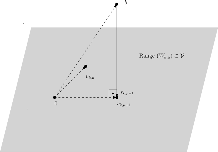
Figure 1: Graphical illustration of an ALS micro-step for the case when $A=\mbox{id}$. At the current iteration step, we define the linear map $W_{k,\mu}\in L(P_{\mu},\mathcal{V})$ by means of $v_{k,\mu}$ and the multilinearity of U, cf. Definition 3.2. The successor $v_{k,\mu+1}$ is then the best approximation of $b$ on the subspace $\mbox{\rm range}\left(W_{k,\mu}\right)\subseteq\mathcal{V}$.

Remark 3.8.

From the definition of $p_{\mu}^{k+1}$, it follows directly that $p_{\mu}^{k+1}\perp\mbox{\rm kernel}(W_{\mu,k})$ and $p_{\mu}^{k+1}$ is the vector with smallest norm that fulfils the normal equation $G_{k,\mu}\,p_{\mu}^{k+1}=W_{k,\mu}^{T}b$. This is very important for the convergence analysis of the ALS method and we like to point out that our results are based on this condition. We must give special attention in a correct implementation of an ALS micro-step in order to fulfil this essential property.

4 Convergence Analysis

We consider global convergence of the ALS method. The convergence analysis for an arbitrary tensor format representation $U:\mathop{\mathchoice{\raise-2.20001pt\hbox{\huge$\times$}}{\raise-0.50003pt\hbox{\Large$\times$}}{\hbox{\large$\times$}}{\times}}_{\mu=1}^{L}P_{\mu}\rightarrow\mathcal{V}$ is a quite challenging task. The objective function $F$ from Eq. (2) is highly nonlinear. Even the existence of a minimum is in general not ensured, see [5] and [22]. We need further assumptions on the sequence from the ALS method. In order to justify our assumptions, let us study an example from Lim and de Silva [5] where it is shown that the tensor

$$b=x\otimes x\otimes y+x\otimes y\otimes x+y\otimes x\otimes x$$

with tensor rank $3$ has no best tensor rank $2$ approximation. Lim and de Silva explained this by constructing a sequence $(v_{k})_{k\in\mathds{N}}$ of rank $2$ tensors with

$$v_{k}=\left(x+\frac{1}{k}\,y\right)\otimes\left(x+\frac{1}{k}\,y\right)\otimes\left(kx+y\right)-x\otimes x\otimes kx\xrightarrow[k\rightarrow\infty]{}b.$$

The linear map $W_{1,k}$ from Definition 3.2 and the first component vector $p_{1,k}$ of the parameter system have the following form:

$$W_{1,k} = \left[\underbrace{\left(x+\frac{1}{k}y\right)\otimes\left(x+\frac{1}{k}y\right),\,x\otimes x}_{\mbox{column vectors of the matrix}}\right]\otimes\mbox{\bf Id}_{\mathds{R}^{n}},$$

$$p_{1}^{k} = \left(\begin{array}[]{c}1\\ 0\\ \end{array}\right)\otimes(kx+y)+\left(\begin{array}[]{c}0\\ 1\\ \end{array}\right)\otimes kx.$$

It is easy to verify that the equation $W_{1,k}p_{1}^{k}=v_{k}$ holds. Furthermore, we have

$$\lim_{k\rightarrow\infty}\|p_{1}^{k}\| = \infty,$$

$$W_{1}=\lim_{k\rightarrow\infty}W_{1,k} = \left(\begin{array}[]{cc}x\otimes x&x\otimes x\\ \end{array}\right)\otimes\mbox{\bf Id}_{\mathds{R}^{n}}.$$

Obviously, the rank of $W_{1}$ is equal to $n$ but $\mbox{\rm rank}(W_{1,k})=2n$ for all $k\in\mathds{N}$. This example shows already that we need assumptions on the boundedness of the parameter system and on the dimension of the subspace $\mbox{\rm span}(W_{\mu,k})$.

Definition 4.1 (Critical Points).

The set $\mathfrak{M}$ of critical points is defined by

$$\mathfrak{M}:=\left\{v\in\mathcal{V}\,:\,\exists\underline{p}\in P:v=U(\underline{p})\wedge F^{\prime}(\underline{p})=0\right\}.$$ (12)

In our context, critical points are tensors that can be represented in our tensor format $U$ and there exists a parameter system $\underline{p}$ such that $(f\circ U)^{\prime}(\underline{p})=0$, i.e. $\underline{p}$ is a stationary point of $F=f\circ U$. A representation system of a tensor $v=U(\underline{p})$ is never uniquely defined since the tensor format is a multilinear map. The following remark shows that the non uniqueness of a parameter system has even more subtle effects, in particular when the parameter system of $v=U(\underline{p})$ is also a stationary point of $F$.

Remark 4.2.

In general, $v\in\mathfrak{M}$ does not imply $F^{\prime}(\hat{p})=0$ for any parameter system $\hat{p}$ of $v$, i.e. there exist a tensor format $\tilde{U}$ and two different $p,\,\hat{p}\in P$ such that $\tilde{U}(p)=\tilde{U}(\hat{p})$ and $0=\tilde{F}^{\prime}(p)\neq\tilde{F}^{\prime}(\hat{p})$.

Proof.

Let

$$\tilde{U}:\mathds{R}^{2}\times\mathds{R}^{2} \rightarrow \mathds{R}^{2}\otimes\mathds{R}^{2}\simeq\mathds{R}^{4}$$

$$(x,y) \mapsto \tilde{U}(x,y):=\left(\begin{array}[]{c}x_{1}y_{1}+x_{2}y_{1}\\ x_{1}y_{1}+x_{2}y_{1}\\ x_{1}y_{2}\\ x_{2}y_{2}\\ \end{array}\right).$$

Obviously, $\tilde{U}$ is a bilinear map. Further, let $b=\left(\begin{array}[]{c}1\\ 1\\ 0\\ 1\\ \end{array}\right)$, $A=\mbox{\bf Id}$ in the definition of $F$ from Eq. (2), and $e_{1}$ and $e_{2}$ the canonical vectors in $\mathds{R}^{2}$, i.e.

$$e_{1}=\left(\begin{array}[]{c}1\\ 0\\ \end{array}\right),\ \ \ \ \ e_{2}=\left(\begin{array}[]{c}0\\ 1\\ \end{array}\right).$$

Then the following holds

• $\tilde{U}(e_{1},e_{1})=\tilde{U}(e_{2},e_{1})$,

• $F^{\prime}(e_{1},e_{1})=0$,

• $F^{\prime}(e_{2},e_{1})\neq 0$.

Elementary calculations result in

$$\tilde{U}(e_{1},e_{1})=\tilde{U}(e_{2},e_{1})=\left(\begin{array}[]{c}1\\ 1\\ 0\\ 0\\ \end{array}\right).$$

The definition of $F$ from Eq. (2) gives

$$F(x,y)=\frac{1}{3}(\frac{1}{2}(2(y_{1}(x_{1}+x_{2}))^{2}+(x_{1}y_{2})^{2}+(x_{2}y_{2})^{2})-2(x_{1}+x_{2})y_{1}-x_{2}y_{2}).$$

Then

$$F(x,e_{1}) = \frac{1}{3}((x_{1}+x_{2})^{2}-2(x_{1}+x_{2})),\,F(e_{1},y)=\frac{1}{3}(y_{1}^{2}+\frac{1}{2}y_{2}^{2}-2y_{1})$$

$$F(e_{2},y) = \frac{1}{3}(y_{1}^{2}+\frac{1}{2}y_{2}^{2}-2y_{1}-y_{2}).$$

and

$$F^{\prime}_{x}(x,e_{1})=\left(\begin{array}[]{c}\frac{2(x_{1}+x_{2}-1)}{3}\\ \frac{2(x_{1}+x_{2}-1)}{3}\\ \end{array}\right),\ \ \ \ \ F^{\prime}_{y}(e_{1},y)=\left(\begin{array}[]{c}\frac{2(y_{1}-1)}{3}\\ \frac{y_{2}}{3}\\ \end{array}\right),\ \ \ \ \ F^{\prime}_{y}(e_{2},y)=\left(\begin{array}[]{c}\frac{2(y_{1}-1)}{3}\\ \frac{y_{2}-1}{3}\\ \end{array}\right).$$

One verifies that $F^{\prime}(e_{1},e_{1})=\left(\begin{array}[]{c}0\\ 0\\ 0\\ 0\\ \end{array}\right)$ and $F^{\prime}(e_{2},e_{1})=\left(\begin{array}[]{c}0\\ 0\\ 0\\ -\frac{1}{3}\\ \end{array}\right)$. ∎

For a convenient understanding, let us briefly repeat the notations from the ALS method, see Algorithm 2. Let $\mu\in\mathds{N}_{L}\cup\{0\}$, $k\in\mathds{N}$, and

$$\underline{p}_{k,\mu} = (p_{1}^{k+1},\dots,p_{\mu-1}^{k+1},p_{\mu}^{k},\dots p_{L}^{k})\in P,$$ (14)

$$v_{k,\mu} = U(\underline{p}_{k,\mu})=U(p_{1}^{k+1},\dots,p_{\mu-1}^{k+1},p_{\mu}^{k},\dots p_{L}^{k})\in\mathcal{V}$$

be the elements of the sequences $(\underline{p}_{k,\mu})_{k\in\mathds{N}}$ and $(v_{k,\mu})_{k\in\mathds{N}}$ from the ALS algorithm. Note that $\underline{p}_{k}=\underline{p}_{k,0}=(p_{1}^{k},\dots,p_{L}^{k})$ and $v_{k}=U(\underline{p}_{k})$.

Definition 4.3 ($\mathcal{A}(v_{k})$).

The set of accumulation points of $(v_{k})_{k\in\mathds{N}}$ is denoted by $\mathcal{A}(v_{k})$, i.e.

$$\mathcal{A}(v_{k}):=\left\{v\in\mathcal{V}:v\mbox{ is an accumulation point of }(v_{k})_{k\in\mathds{N}}\right\}.$$ (15)

We demonstrate in Theorem 4.13 that every accumulation point of $(v_{k})_{k\in\mathds{N}}$ is a critical point, i.e. $\mathcal{A}(v_{k})\subseteq\mathfrak{M}$. This is an existence statement on the parameter space $P$. Lemma 4.5 shows us a candidate for such a parameter system.

Remark 4.4.

Obviously, if the sequence of parameter $(\underline{p}_{k})_{k\in\mathds{N}}$ is bounded, then the set of accumulation points of $(\underline{p}_{k})_{k\in\mathds{N}}$ is not empty. Consequently, the set $\mathcal{A}(v_{k})$ is not empty, since the tensor format $U$ is a continuous map.

Lemma 4.5.

Let the sequence $(\underline{p}_{k})_{k\in\mathds{N}}$ from the ALS method be bounded and define for $J\subseteq\mathds{N}$ the following set of accumulation points:

$$\mathcal{A}_{J}:=\bigcup_{\mu=0}^{L-1}\left\{\underline{p}\in P:\underline{p}\mbox{ is an accumulation point of }(\underline{p}_{k,\mu})_{k\in J}\right\}.$$

There exists $\underline{p}^{*}=(p^{*}_{1},\dots,p^{*}_{L})\in\mathcal{A}_{J}$ such that

$$\|\underline{p}^{*}\|=\min_{\underline{p}\in\mathcal{A}_{J}}\|\underline{p}\|.$$

Proof.

Since the sequence $(\underline{p}_{k})_{k\in\mathds{N}}$ is bounded, it follows from the definition in Eq. (14) that $(\underline{p}_{k,\mu})_{k\in\mathds{N}}$ is also bounded. Therefore the set $\left\{\underline{p}\in P:\underline{p}\mbox{ is an accumulation point of }(\underline{p}_{k,\mu})_{k\in J}\right\}$ is not empty and compact. Hence $\mathcal{A}$ is a compact and non-empty set. ∎

We are now ready to establish our main assumptions on the sequence from the ALS method.

Assumption 4.6.

During the article, we say that $(\underline{p}_{k})_{k\in\mathds{N}}$ satisfies assumption A1 or assumption A2 if the following holds true:

• The sequence $(\underline{p}_{k})_{k\in\mathds{N}}$ is bounded.

• The sequence $(\underline{p}_{k})_{k\in\mathds{N}}$ is bounded and for $J\subseteq\mathds{N}$ we have

  $$\forall\mu\in\mathds{N}_{L}:\exists k_{0}\in J:\forall k\in J:\quad k\geq k_{0}\quad\Rightarrow\quad\mbox{\rm rank}(W_{k,\mu})=\mbox{\rm rank}(W^{*}_{\mu}),$$ (16)

  where $\underline{p}^{*}=(p^{*}_{1},\dots,p^{*}_{L})\in\mathcal{A}_{J}$ is a accumulation point form Lemma 4.5 and

  $$W_{k,\mu} = W_{\mu}(p_{1}^{k+1},\dots p_{\mu-1}^{k+1},p_{\mu+1}^{k},\dots,p_{L}^{k}),$$

  $$W^{*}_{\mu} = W_{\mu}(p_{1}^{*},\dots p_{\mu-1}^{*},p_{\mu+1}^{*},\dots,p_{L}^{*}).$$

Remark 4.7.

In the proof of Theorem 4.13, assumption A2 ensures that the ALS method depends continuously on the parameter system $\underline{p}_{k,\mu}$, i.e. $G_{k,\mu}^{+}W^{T}_{k,\mu}b\xrightarrow[k\rightarrow\infty]{}G^{+}_{\mu}W_{\mu}^{T}b$ for a convergent subsequence $(\underline{p}_{k,\mu})_{k\in J}$.

Using the notations and definitions from Section 3, we define further

$$A_{k,\mu} := V_{k,\mu}^{T}AV_{k,\mu},$$ (17)

for $k\in\mathds{N}$ and $\mu\in\mathds{N}_{L}$.

For the ALS method there is an explicit formula for the decay of the values between $f(v_{k,\,\mu+1})$ and $f(v_{k,\,\mu})$. The relation between the function values from Eq. (18) is crucial for the convergence analysis of the ALS method.

Lemma 4.8.

Let $k\in\mathds{N}$, $\mu\in\mathds{N}_{L}$. We have

$$f(v_{k,\,\mu+1})-f(v_{k,\mu})=-\frac{1}{2}\frac{\left\langle V_{k,\mu}A_{k,\mu}^{-1}V_{k,\mu}^{T}r_{k,\mu},r_{k,\mu}\right\rangle}{\|b\|^{2}}$$ (18)

Proof.

From Algorithm 2, we have that $v_{k,\mu+1}=v_{k,\mu}+\Delta_{k,\mu}$, where $\Delta_{k,\mu}:=V_{k,\mu}A_{k,\mu}^{-1}V_{k,\mu}^{T}r_{k,\mu}$. Elementary calculations give

$$f(v_{k,\mu+1}) = \frac{1}{\|b\|^{2}}\left[\left\langle A(v_{k,\mu}+\Delta_{k,\mu}),v_{k,\mu}+\Delta_{k,\mu}\right\rangle-\left\langle b,v_{k,\mu}+\Delta_{k,\mu}\right\rangle\right]$$

$$= f(v_{k,\mu})+\frac{-\left\langle r_{k,\,\mu},\Delta_{k,\,\mu}\right\rangle+\frac{1}{2}\left\langle A\Delta_{k,\,\mu},\Delta_{k,\,\mu}\right\rangle}{\|b\|^{2}}$$

$$= f(v_{k,\mu})+\frac{-\left\langle V_{k,\mu}A_{k,\mu}^{-1}V_{k,\mu}^{T}r_{k,\,\mu},r_{k,\,\mu}\right\rangle+\frac{1}{2}\left\langle AV_{k,\mu}A_{k,\mu}^{-1}V_{k,\mu}^{T}r_{k,\mu},V_{k,\mu}A_{k,\mu}^{-1}V_{k,\mu}^{T}r_{k,\mu}\right\rangle}{\|b\|^{2}}$$

$$= f(v_{k,\mu})+\frac{-\left\langle V_{k,\mu}A_{k,\mu}^{-1}V_{k,\mu}^{T}r_{k,\,\mu},r_{k,\,\mu}\right\rangle+\frac{1}{2}\left\langle V_{k,\mu}A_{k,\mu}^{-1}V_{k,\mu}^{T}r_{k,\,\mu},r_{k,\,\mu}\right\rangle}{\|b\|^{2}}$$

$$= f(v_{k,\mu})-\frac{1}{2\|b\|^{2}}\left\langle V_{k,\mu}A_{k,\mu}^{-1}V_{k,\mu}^{T}r_{k,\,\mu},r_{k,\,\mu}\right\rangle.$$

∎

Corollary 4.9.

$(f(v_{k}))_{k\in\mathds{N}}\subset\mathds{R}$ is a descending sequence and there exists $\alpha\in\mathds{R}$ such that $f(v_{k})\xrightarrow[k\rightarrow\infty]{}\alpha$.

Proof.

Let $k\in\mathds{N}$ and $\mu\in\mathds{N}_{L}$. From Lemma 4.8 it follows that

$$f(v_{k+1})-f(v_{k}) = f(v_{k,L})-f(v_{k,0})=\sum_{\mu=1}^{L}f(v_{k,\,\mu})-f(v_{k,\mu-1})$$

$$= -\frac{1}{2\|b\|^{2}}\sum_{\mu=0}^{L-1}\left\langle A_{k,\mu}^{-1}V_{k,\mu}^{T}r_{k,\mu},V_{k,\mu}^{T}r_{k,\mu}\right\rangle\leq 0,$$

since the matrices $A_{k,\mu}^{-1}$ are positive definite. This shows that $(f(v_{k}))_{k\in\mathds{N}}\subset\mathds{R}$ is a descending sequence. The sequence of function values $(f(v_{k}))_{k\in\mathds{N}}$ is bounded from below, since the matrix $A$ in the definition of $f$ is positive definite. Therefore, there exists an $\alpha\in\mathds{R}$ such that $f(v_{k})\xrightarrow[k\rightarrow\infty]{}\alpha$. ∎

Lemma 4.10.

Let $(v_{k,\mu})_{k\in\mathds{N},\mu\in\mathds{N}_{L}}\subset\mathcal{V}$ be the sequence from Algorithm 2. We have

$$f(v_{k,\mu})=-\frac{1}{2\|b\|^{2}}\left\langle v_{k,\mu},b\right\rangle=-\frac{1}{2\|b\|^{2}}\|v_{k,\mu}\|^{2}_{A}$$ (19)

for all $k\in\mathds{N},\mu\in\mathds{N}_{L}$, where $\left\langle v,w\right\rangle_{A}:=\left\langle Av,w\right\rangle$ and $\|v\|_{A}:=\sqrt{\left\langle v,v\right\rangle_{A}}$.

Proof.

Let $k\in\mathds{N}$ and $\mu\in\mathds{N}_{L}$. We have

$$\left\langle v_{k,\mu},v_{k,\mu}\right\rangle_{A} = \left\langle AV_{k,\mu-1}\left(V_{k,\mu-1}^{T}AV_{k,\mu-1}\right)^{-1}V_{k,\mu-1}^{T}b,V_{k,\mu-1}\left(V_{k,\mu-1}^{T}AV_{k,\mu-1}\right)^{-1}V_{k,\mu-1}^{T}b\right\rangle$$

$$= \left\langle V_{k,\mu-1}^{T}b,\left(V_{k,\mu-1}^{T}AV_{k,\mu-1}\right)^{-1}V_{k,\mu-1}^{T}b\right\rangle=\left\langle v_{k,\mu},b\right\rangle.$$

The rest follows from the definition of $f$, see Eq. (1). ∎

Corollary 4.11.

Let $(v_{k,\mu})_{k\in\mathds{N},\mu\in\mathds{N}_{L}}\subset\mathcal{V}$ be the sequence of represented tensors from the ALS algorithm. The following holds:

• $f(v_{k,\mu+1})\leq f(v_{k,\mu})$,

• $\|v_{k,\mu+1}\|^{2}_{A}\geq\|v_{k,\mu}\|^{2}_{A}$,

• $\left\langle v_{k,\mu+1},b\right\rangle\geq\left\langle v_{k,\mu},b\right\rangle$.

Proof.

Follows from Lemma 4.9 and Lemma 4.10. ∎

Lemma 4.12.

Let the sequence $(\underline{p}_{k})_{k\in\mathds{N}}\subset P$ fulfil the assumption A1. Then we have

$$\max_{0\leq\mu\leq L-1}\left\|F_{\mu}^{\prime}(p_{\mu}^{k})\right\|\xrightarrow[k\rightarrow\infty]{}0.$$

Proof.

According to Lemma 3.6 and Lemma 4.8, we have

$$f(v_{k})-f(v_{k+1}) = \sum_{\mu=1}^{L}f(v_{k,\mu-1})-f(v_{k,\,\mu})=\frac{1}{2\|b\|^{2}}\sum_{\mu=0}^{L-1}\left\langle A_{k,\mu}^{-1}V_{k,\mu}^{T}r_{k,\mu},V_{k,\mu}^{T}r_{k,\mu}\right\rangle$$

$$= \frac{1}{2\|b\|^{2}}\sum_{\mu=0}^{L-1}\left\langle A_{k,\mu}^{-1}\left(\tilde{U}_{k,\mu}\tilde{D}^{-\frac{1}{2}}_{k\mu}\right)^{T}W_{k,\mu}^{T}r_{k,\mu},\left(\tilde{U}_{k,\mu}\tilde{D}^{-\frac{1}{2}}_{k\mu}\right)^{T}W^{T}_{k,\mu}r_{k,\mu}\right\rangle$$

$$= \frac{1}{2\|b\|^{2}}\sum_{\mu=0}^{L-1}\left\langle A_{k,\mu}^{-1}\left(\tilde{U}_{k,\mu}\tilde{D}^{-\frac{1}{2}}_{k\mu}\right)^{T}F^{\prime}_{\mu}(p_{\mu}^{k}),\left(\tilde{U}_{k,\mu}\tilde{D}^{-\frac{1}{2}}_{k\mu}\right)^{T}F^{\prime}_{\mu}(p_{\mu}^{k})\right\rangle$$

$$\geq \frac{1}{2\|b\|^{2}}\sum_{\mu=0}^{L-1}\lambda_{\min}(A^{-1}_{k,\mu})\lambda_{\min}\left(\tilde{U}_{k,\mu}\tilde{D}^{-1}_{k\mu}\tilde{U}_{k,\mu}^{T}\right)\left\|F_{\mu}^{\prime}(p_{\mu}^{k})\right\|^{2}$$

$$\geq \frac{1}{2\lambda_{\max}(A)\|b\|^{2}}\sum_{\mu=0}^{L-1}\lambda_{\min}\left(\tilde{U}_{k,\mu}\tilde{D}^{-1}_{k\mu}\tilde{U}_{k,\mu}^{T}\right)\left\|F_{\mu}^{\prime}(p_{\mu}^{k})\right\|^{2},$$

where $V_{k,\mu}=W_{k,\mu}\tilde{U}_{k,\mu}\tilde{D}^{-\frac{1}{2}}_{k\mu}$ is from Eq. (6). In the last estimate, we have used that the Ritz values are bounded by the smallest and largest eigenvalue of $A$, i.e $\lambda_{\min}(A)\leq\lambda_{\min}(A_{k,\mu})\leq\lambda_{\max}(A_{k,\mu})\leq\lambda_{\max}(A)$. Since the tensor format $U$ is continues and the sequence $(\underline{p}_{k})_{k\in\mathds{N}}$ is bounded, it follows from the theorem of Gershgorin and Cauchy-Schwarz inequality that there is $\gamma>0$ such that $\lambda_{\max}\left(W_{k,\mu}^{T}W_{k,\mu}\right)\leq\gamma$, recall that $W_{k,\mu}^{T}W_{k,\mu}=\tilde{U}_{k,\mu}D_{k,\mu}\tilde{U}^{T}_{k,\mu}$, see Proposition 3.3. Therefore, we have

$$f(v_{k})-f(v_{k+1})\geq\frac{1}{2\lambda_{\max}(A)\gamma\|b\|^{2}}\sum_{\mu=0}^{L-1}\left\|F_{\mu}^{\prime}(p_{\mu}^{k})\right\|^{2}\geq\frac{1}{2\lambda_{\max}(A)\gamma\|b\|^{2}}\max_{0\leq\mu\leq L-1}\left\|F_{\mu}^{\prime}(p_{\mu}^{k})\right\|^{2}\geq 0.$$

Further, it follows from Corollary 4.9 that

$$0=\lim_{k\rightarrow\infty}\sqrt{f(v_{k})-f(v_{k+1})}=\lim_{k\rightarrow\infty}\max_{0\leq\mu\leq L-1}\left\|F_{\mu}^{\prime}(p_{\mu}^{k})\right\|.$$

∎

Theorem 4.13.

Let $(v_{k})_{k\in\mathds{N}}$ be the sequence of represented tensors and suppose that the sequence of parameter $(\underline{p}_{k})_{k\in\mathds{N}}\subset P$ from the ALS method fulfils assumption A2. Every accumulation point of $(v_{k})_{k\in\mathds{N}}$ is a critical point, i.e. $\mathcal{A}(v_{k})\subseteq\mathfrak{M}$. Further, we have

$$\mbox{\rm dist}\left(v_{k},\mathfrak{M}\right)\xrightarrow[k\rightarrow\infty]{}0.$$

Proof.

Let $\bar{v}\in\mathcal{A}(v_{k})$ be an accumulation point and $(v_{k})_{k\in J\subseteq\mathds{N}}\subset U(P)$ a subsequence in the range set of the tensor format $U$ with $v_{k}\xrightarrow[k\rightarrow\infty]{}\bar{v}$. Then there exists $(p_{k})_{k\in J\subseteq\mathds{N}}\subset P$ with $v_{k}=U(p_{k})$ for all $k\in J$. Further, let $\mu\in\mathds{N}_{L}$ and define for all $k\in J$

$$\underline{g}_{k,\mu}:=(p_{1}^{k+1},\dots,p_{\mu}^{k+1},p_{\mu+1}^{k},\dots,p_{L}^{k})\in P.$$

Let $\mu^{*}\in\mathds{N}_{L}$ and $(g_{k,\mu^{*}})_{k\in J^{\prime}\subseteq J}$ with $g_{k,\mu^{*}}\xrightarrow[k\rightarrow\infty]{}\underline{p}^{*}:=\mbox{\rm argmax}_{\underline{p}\in\mathcal{A}_{J}}\|\underline{p}\|\in P$, see Lemma 4.5. Without loss of generality, let us assume that $\mu^{*}=1$. This assumption makes the the notations not more complicated then necessary. Since $(g_{k,\mu})_{k\in J}$ is bounded, there exists $\underline{p}^{[\mu]}\in P$ and a corresponding subsequence $(\underline{g}_{k,\mu})_{k\in J_{\mu}\subseteq J}$ such that

$$\underline{p}_{k}=\underline{g}_{k,0} = (p_{1}^{k},p_{2}^{k},\dots,p_{L}^{k})\xrightarrow[k\rightarrow\infty]{}\underline{p}^{*}=(p_{1},p_{2},\dots,p_{L}),$$

$$\underline{g}_{k,1} = (p_{1}^{k+1},p_{2}^{k},\dots,p_{L}^{k})\xrightarrow[k\rightarrow\infty]{}\underline{p}^{[1]}=(\tilde{p}_{1},p_{2},\dots,p_{L}),$$

$$\underline{g}_{k,\mu} = (p_{1}^{k+1},\dots,p_{\mu}^{k+1},p_{\mu+1}^{k},\dots,p_{L}^{k})\xrightarrow[k\rightarrow\infty]{}\underline{p}^{[\mu]}=(\tilde{p}_{1},\dots,\tilde{p}_{\mu},p_{\mu+1},\dots,p_{L}),$$

$$\underline{g}_{k,L} = (p_{1}^{k+1},\dots,p_{L}^{k+1})\xrightarrow[k\rightarrow\infty]{}\underline{p}^{[L]}=(\tilde{p}_{1},\dots,\tilde{p}_{L}).$$

From Lemma 4.15 and $U(\underline{p}_{k})\xrightarrow[k\rightarrow\infty]{}\bar{v}$ it follows that

$$\bar{v} = \lim_{k\rightarrow\infty}U(\underline{g}_{k,\mu})=U(\underline{p}^{[\mu]})\quad\mbox{f.a. }\mu\in\mathds{N}_{L},$$ (20)

where $k\in J$. Furthermore, we have

$$\underline{p}^{*}=\underline{p}^{[1]}=\dots=\underline{p}^{[L]}.$$

To show this, assume that

$$M:=\left\{\mu\in\mathds{N}_{L}:\underline{p}^{[\mu]}\neq\underline{p}^{*}\right\}\neq\emptyset$$

and define $\nu:=\min M\in\mathds{N}_{L}$. From assumption A2 it follows

$$p_{\nu}^{k+1}=G_{k,\nu}^{+}W^{T}_{k,\nu}b\xrightarrow[k\rightarrow\infty]{}G^{+}_{\nu}W_{\nu}^{T}b=\tilde{p}_{\nu}.$$

Thus we have in particular that $\tilde{p}_{\nu}\bot\mbox{\rm kernel}W_{\nu}$, see the Definition of $G^{+}_{\nu}$ and Proposition 3.3. Since $U(\underline{p}^{*})=U(\underline{p}^{[\nu]})\Leftrightarrow W_{\nu}p_{\nu}=W_{\nu}\tilde{p}_{\nu}$, it follows further that $\delta_{\nu}:=p_{\nu}-\tilde{p}_{\nu}\in\mbox{\rm kernel}W_{\nu}$ and $\|p_{\nu}\|^{2}=\|\tilde{p}_{\nu}\|^{2}+\|\delta_{\nu}\|^{2}$. Lemma 3.6 and Lemma 4.12 show that

$$W_{k,\nu}^{T}(AW_{k,\nu}p_{\nu}^{k}-b)\xrightarrow[k\rightarrow\infty]{}0.$$

From the definition of $\nu$, we have then

$$W_{\nu}^{T}(AW_{\nu}p_{\nu}-b)=0,$$

note that for $\nu=\min M$

$$\underline{g}_{k,\nu}=(p_{1}^{k+1},\dots,p_{\nu}^{k+1},p_{\nu+1}^{k},\dots,p_{L}^{k})\xrightarrow[k\rightarrow\infty]{}\underline{p}^{[\nu]}=(p_{1},\dots,p_{\nu-1},\tilde{p}_{\nu},p_{\nu+1},\dots,p_{L})$$

holds. Since $\tilde{p}_{\nu}=G^{+}_{\nu}W_{\nu}^{T}b$ and $\underline{p}^{*}=\mbox{\rm argmin}_{\underline{p}\in\mathcal{A}_{J}}\|\underline{p}\|$, it follows $\|\tilde{p}_{\nu}\|=\|p_{\nu}\|$. Hence, we have $\tilde{p}_{\nu}=p_{\nu}$, because $\|p_{\nu}\|^{2}=\|\tilde{p}_{\nu}\|^{2}+\|\delta_{\nu}\|^{2}$ implies then $\delta_{\nu}=0$. But $\tilde{p}_{\nu}=p_{\nu}$ contradicts the definition of $\nu=\min M$. Consequently, we have

$$\underline{p}^{*}=\underline{p}^{[1]}=\dots=\underline{p}^{[L]}.$$

From Eq. (20) and the definition of $p_{\mu}^{k+1}$ it follows then

$$\bar{v}=U(\underline{p}^{*})$$

and

$$0=\lim_{k\rightarrow\infty}F^{\prime}_{\mu}(\underline{g}_{k,\mu})=F^{\prime}_{\mu}(\underline{p}^{*})\quad\mbox{ for all }\mu\in\mathds{N}_{L},$$

i.e. $\mathcal{A}(v_{k})\subseteq\mathfrak{M}$. Now, let $\delta_{k}=\inf_{v\in\mathfrak{M}}\|v_{k}-v\|$ and suppose that there exists a subsequence $(\delta_{k})_{k\in J\subseteq\mathds{N}}$ with $\lim_{k\rightarrow\infty}\delta_{k}=\delta\in\mathds{R}_{+}$. Then $(v_{k})_{k\in J}$ has a convergent subsequence. Since this subsequence must have its limit point in $\mathfrak{M}$, it follows that $\delta=0$. Which proves $\mbox{\rm dist}\left(v_{k},\mathfrak{M}\right)\xrightarrow[k\rightarrow\infty]{}0$ by contradiction.

∎

Lemma 4.14.

Let $(v_{k})_{k\in\mathds{N}}\subset\mathcal{V}$ be the sequence of represented tensors from the ALS method. It holds

$$\|v_{k+1}-v_{k}\|_{A}\xrightarrow[k\rightarrow\infty]{}0.$$

Proof.

Let $k\in\mathds{N}$. We have

$$\|v_{k+1}-v_{k}\|_{A}^{2} = \left\|\sum_{\mu=1}^{L}v_{k,\mu}-v_{k,\mu-1}\right\|^{2}_{A}\leq\left(\sum_{\mu=1}^{L}\|v_{k,\mu}-v_{k,\mu-1}\|_{A}\right)^{2}\leq L\sum_{\mu=0}^{L-1}\left\|v_{k,\mu+1}-v_{k,\mu}\right\|^{2}_{A}.$$ (21)

Since $v_{k,\mu+1}-v_{k,\mu}=V_{k,\mu}A_{k,\mu}^{-1}V_{k,\mu}^{T}r_{k,\mu}$, it follows further

$$\left\|v_{k,\mu+1}-v_{k,\mu}\right\|^{2}_{A} = \left\|V_{k,\mu}A_{k,\mu}^{-1}V_{k,\mu}^{T}r_{k,\mu}\right\|^{2}_{A}=\left\langle AV_{k,\mu}A_{k,\mu}^{-1}V_{k,\mu}^{T}r_{k,\mu},V_{k,\mu}A_{k,\mu}^{-1}V_{k,\mu}^{T}r_{k,\mu}\right\rangle$$

$$= \left\langle A_{k,\mu}^{-1}V_{k,\mu}^{T}r_{k,\mu},V^{T}_{k,\mu}AV_{k,\mu}A_{k,\mu}^{-1}V_{k,\mu}^{T}r_{k,\mu}\right\rangle=\left\langle A_{k,\mu}^{-1}V_{k,\mu}^{T}r_{k,\mu},V_{k,\mu}^{T}r_{k,\mu}\right\rangle$$

$$= \left\langle V_{k,\mu}A_{k,\mu}^{-1}V_{k,\mu}^{T}r_{k,\mu},r_{k,\mu}\right\rangle.$$

Combining this with Eq. (18) and (21) gives

$$\|v_{k+1}-v_{k}\|_{A}^{2} \leq 2L\|b\|^{2}\sum_{\mu=0}^{L-1}\left(f(v_{k,\mu})-f(v_{k,\mu+1})\right)=2L\|b\|^{2}\left(f(v_{k})-f(v_{k+1})\right).$$

From Corollary 4.9 it follows $\left(f(v_{k})-f(v_{k})\right)\xrightarrow[k\rightarrow\infty]{}0$. Therefore, we have

$$\|v_{k+1}-v_{k}\|_{A}\xrightarrow[k\rightarrow\infty]{}0.$$

∎

Lemma 4.15.

Let $(v_{k})_{k\in\mathds{N}}\subset\mathcal{V}$ be the sequence of tensors from the ALS method and $\bar{v}\in\mathcal{V}$ with $\lim_{k\rightarrow\infty}v_{k}=\bar{v}$. Further, let $\mu\in\mathds{N}_{L}$ and $(v_{k,\mu})_{k\in\mathds{N}}\subset\mathcal{V}$ as defined in Algorithm 2. We have

$$\lim_{k\rightarrow\infty}v_{k,\mu}=\bar{v}\quad\mbox{for all }\mu\in\mathds{N}_{L}.$$

Proof.

Define $v_{k,0}:=v_{k}$ (like in Algorithmus 2) and assume that

$$M:=\left\{\mu\in\mathds{N}_{L}:\lim_{k\rightarrow\infty}v_{k,\mu}\neq\bar{v}\right\}\neq\emptyset.$$

Furthermore, set $\mu^{*}:=\min M\in\mathds{N}_{L}$.

From Lemma 4.14 it follows

$$\|v_{k,\mu^{*}}-\bar{v}\|_{A}\leq\|v_{k,\mu^{*}}-v_{\mu^{*}-1,k}\|_{A}+\|v_{k,\mu^{*}-1}-\bar{v}\|_{A}\xrightarrow[k\rightarrow\infty]{}0.$$

But this contradicts the definition of $\mu^{*}$. ∎

In the following, the dimension of the tensor space $\mathcal{V}=\bigotimes_{\mu=1}^{d}\mathds{R}^{m_{\mu}}$ is denoted by $N\in\mathds{N}$, i.e. $N=\prod_{\mu=1}^{d}m_{\mu}$. The statement of Lemma 4.20 delivers an explicit recursion formula for the tangent of the angle between iteration points and an arbitrary tensor. This result is important for the rate of convergence of the ALS algorithm.

Lemma 4.16.

Let $\mu,\nu\in\mathds{N}_{L}$, $\nu\neq\mu$, and $\underline{p}=(p_{1},\dots,p_{\nu},\dots,p_{\mu},\dots,p_{L})\in P$. There exists a multilinear map $M_{\mu,\nu}:P_{1}\times\dots\times P_{\nu-1}\times P_{\nu+1}\times\dots\times P_{\mu-1}\times P_{\mu+1}\times\dots\times P_{L}\times\mathcal{V}\rightarrow L(P_{\nu},P_{\mu})$ such that

$$W^{T}_{\mu}(p_{1},\dots,\mathbf{g_{\nu}},\dots,p_{\mu-1},p_{\mu+1},\dots,p_{L})b=M_{\mu,\nu}(p_{1},\dots,p_{\nu-1},p_{\nu+1},\dots,p_{\mu-1},p_{\mu+1},\dots,p_{L},b)\mathbf{g_{\nu}}$$ (22)

for all $\mathbf{g_{\nu}}\in P_{\nu}$. Moreover, we have

$$M_{\mu,\nu}(p_{1},\dots,p_{\nu-1},p_{\nu+1},\dots,p_{\mu-1},p_{\mu+1},\dots,p_{L},b)=M^{T}_{\nu,\mu}(p_{1},\dots,p_{\nu-1},p_{\nu+1},\dots,p_{\mu-1},p_{\mu+1},\dots,p_{L},b).$$

Proof.

Follows form Proposition 3.3 (v) and definition of $W^{T}_{\mu}(p_{1},\dots,\mathbf{g_{\nu}},\dots,p_{\mu-1},p_{\mu+1},\dots,p_{L})b$. ∎

Corollary 4.17.

Let $\mu\in\mathds{N}_{L}$, $k\geq 2$, and $\underline{p}_{k,\mu}=(p^{k+1}_{1},\dots,p^{k+1}_{\mu-1},p_{\mu}^{k},p^{k}_{\mu+1},\dots,p_{L}^{k})$ form Algorithm 2. There exists a multilinear map $M_{\mu}:P_{1}\times\dots\times P_{\mu-2}\times P_{\mu+1}\times\dots\times P_{L}\times\mathcal{V}\rightarrow L(P_{\mu-1},P_{\mu})$ such that

$$p^{k+1}_{\mu} = G^{+}_{k,\,\mu}M_{\mu}(p_{1}^{k+1},\dots,p_{\mu-2}^{k+1},p_{\mu+1}^{k},\dots,p_{L}^{k},b)p_{\mu-1}^{k+1},$$ (23)

$$p_{\mu-1}^{k+1} = G^{+}_{k,\,\mu-1}M^{T}_{\mu}(p_{1}^{k+1},\dots,p_{\mu-2}^{k+1},p_{\mu+1}^{k},\dots,p_{L}^{k},b)p_{\mu}^{k},$$ (24)

$$\mbox{ i.e. }p^{k+1}_{\mu} = G^{+}_{k,\,\mu}M_{\mu}(p_{1}^{k+1},\dots,p_{\mu-2}^{k+1},p_{\mu+1}^{k},\dots,p_{L}^{k},b)\,G^{+}_{k,\,\mu-1}M^{T}_{\mu}(p_{1}^{k+1},\dots,p_{\mu-2}^{k+1},p_{\mu+1}^{k},\dots,p_{L}^{k},b)p_{\mu}^{k},$$

where $G^{+}_{k,\,\mu-1}$ and $G^{+}_{k,\,\mu}$ are defined in Algorithm 2.

Proof.

Follows form Eq. (9) and Lemma 4.16. ∎

The following example shows a concrete realisation of the matrix $M_{\mu}$ for the tensor rank-one approximation problem.

Example 4.18.

The approximation of $b\in\mathcal{V}$ by a rank one tensor is considered. Let $v_{k}=p_{1}^{k}\otimes p_{2}^{k}\otimes\dots\otimes p_{d}^{k}$ and

$$b=\sum_{i_{1}=1}^{t_{1}}\dots\sum_{i_{d}=1}^{t_{d}}\beta_{(i_{1},\dots,i_{d})}\bigotimes_{\mu=1}^{d}b_{\mu,i_{\mu}},$$

i.e. the tensor $b$ is given in the Tucker decomposition. From Eq. (9) it follows

$$p_{1}^{k+1} = \frac{1}{\prod_{\mu=2}^{d}\left\|p_{\mu}^{k}\right\|^{2}}\sum_{i_{1}=1}^{t_{1}}\dots\sum_{i_{d}=1}^{t_{d}}\beta_{(i_{1},\dots,i_{d})}\prod_{\mu=2}^{d}\left\langle b_{\mu,i_{\mu}},p_{\mu}^{k}\right\rangle b_{1,i_{1}}$$

$$= \frac{1}{\prod_{\mu=2}^{d-1}\left\|p_{\mu}^{k}\right\|\|p_{d}^{k}\|^{2}}\left[\sum_{i_{1}=1}^{t_{1}}\sum_{i_{d}=1}^{t_{d}}b_{1,i_{1}}\sum_{i_{2}=1}^{t_{2}}\dots\sum_{i_{d-1}=1}^{t_{d-1}}\beta_{(i_{1},\dots,i_{d})}\prod_{\mu=2}^{d-1}\frac{\left\langle b_{\mu,i_{\mu}},p_{\mu}^{k}\right\rangle}{\|p_{\mu}^{k}\|}b^{T}_{d,i_{d}}\right]p_{d}^{k}$$

$$= \frac{1}{\prod_{\mu=2}^{d-1}\left\|p_{\mu}^{k}\right\|\|p_{d}^{k}\|^{2}}\underbrace{B_{1}\Gamma_{1,k}B_{d}^{T}}_{M_{1}(p_{2}^{k},\dots,p_{d-1}^{k})=}p_{d}^{k},$$

where $B_{\mu}=\left(b_{\mu,i_{\mu}}\,:\,1\leq i_{\mu}\leq t_{\mu}\right)\in\mathds{R}^{n_{\mu}\times t_{\mu}}$, $B_{\mu}^{T}B_{\mu}=\mbox{\bf Id}_{\mathds{R}^{t_{\mu}}}$, and the entries of the matrix $\Gamma_{1,k}\in\mathds{R}^{t_{1}\times t_{d}}$ are defined by

$$[\Gamma_{1,k}]_{i_{1},i_{d}}=\sum_{i_{2}=1}^{t_{2}}\dots\sum_{i_{d-1}=1}^{t_{d-1}}\beta_{(i_{1},\dots,i_{d})}\prod_{\mu=2}^{d-1}\frac{\left\langle b_{\mu,i_{\mu}},p_{\mu}^{k}\right\rangle}{\|p_{\mu}^{k}\|}\quad\left(1\leq i_{1}\leq t_{1},\,1\leq i_{d}\leq t_{d}\right).$$

Note that $\Gamma_{1,k}$ is a diagonal matrix if the coefficient tensor $\beta\in\bigotimes_{\mu=1}^{d}\mathds{R}^{t_{\mu}}$ is super- diagonal, see the example in [13]. For $p_{d}^{k}$ it follows further

$$p_{d}^{k} = \frac{1}{\prod_{\mu=1}^{d-1}\left\|p_{\mu}^{k}\right\|^{2}}\sum_{i_{1}=1}^{t_{1}}\dots\sum_{i_{d}=1}^{t_{d}}\beta_{(i_{1},\dots,i_{d})}\prod_{\mu=1}^{d-1}\left\langle b_{\mu,i_{\mu}},p_{\mu}^{k}\right\rangle b_{d,i_{d}}=\frac{1}{\left\|p_{1}^{k}\right\|^{2}\prod_{\mu=2}^{d-1}\left\|p_{\mu}^{k}\right\|}B_{d}\Gamma^{T}_{1,k}B_{1}^{T}p_{1}^{k}$$

and finally

$$p_{1}^{k+1}=\frac{1}{\prod_{\mu=1}^{d}\left\|p_{\mu}^{k}\right\|^{2}}\,B_{1}\Gamma_{1,k}\Gamma^{T}_{1,k}B_{1}^{T}\,p_{1}^{k}.$$

Lemma 4.19.

Let $\mu\in\mathds{N}_{L}$, $(\underline{p}_{k,\mu})_{k\in\mathds{N}}\subset P$, and $\left(v_{k,\mu}\right)_{k\in\mathds{N}}\subset\mathcal{V}$ be the sequences from Algorithm 2. Furthermore, define

$$M_{k,\mu} := M_{\mu}(p_{1}^{k+1},\dots,p_{\mu-2}^{k+1},p_{\mu+1}^{k},\dots,p_{L}^{k},b),$$

$$H_{k,\mu-1} := W^{T}_{k,\mu-1}W_{k,\mu-1},$$

$$N_{k,\mu} := W_{k,\mu}G^{+}_{k,\mu}M_{k,\mu}H^{+}_{k,\mu-1}W^{T}_{k,\mu-1},$$

where we have used the notations from Algorithm 2. A micro-step of the ALS method is described by the following recursion formula:

$$v_{k,\mu+1}=N_{k,\mu}v_{k,\mu}\quad\mbox{ for all }k\geq 2,$$ (25)

i.e.

$$U(p_{1}^{k+1},\dots,p_{\mu-1}^{k+1},p_{\mu}^{k+1},p_{\mu+1}^{k},\dots,p_{L}^{k})=N_{k,\mu}\,U(p_{1}^{k+1},\dots,p_{\mu-1}^{k+1},p_{\mu}^{k},p_{\mu+1}^{k},\dots,p_{L}^{k}).$$

Proof.

According to Corollary 4.17, Remark 3.8, and definition of $v_{k,\mu+1}$, we have that

$$N_{k,\mu}v_{k,\mu} = W_{k,\mu}G^{+}_{k,\mu}M_{k,\mu}H^{+}_{k,\mu-1}W^{T}_{k,\mu-1}W_{k,\mu-1}p_{\mu-1}^{k+1}=W_{k,\mu}G^{+}_{k,\mu}M_{k,\mu}H^{+}_{k,\mu-1}H_{k,\mu-1}p_{\mu-1}^{k+1}$$

$$= W_{k,\mu}G^{+}_{k,\mu}M_{k,\mu}p_{\mu-1}^{k+1}=W_{k,\mu}G^{+}_{k,\mu}W^{T}_{k,\mu}b=W_{k,\mu}p_{\mu}^{k+1}=v_{k,\mu+1}.$$

∎

Lemma 4.20.

Let $\left(N_{k,\mu}\right)_{k\in\mathds{N},\,\mu\in\mathds{N}_{L}}$ be the sequence of matrices from Lemma 4.19, $\bar{v}\in\mathcal{V}\setminus\{0\}$, and $R\in\mathds{R}^{N\times N-1}$ an orthogonal matrix with $\mbox{\rm span}(\bar{v})^{\bot}=\mbox{\rm range}(R)$, i.e. the column vectors of $R$ form an orthonormal basis of the linear space $\mbox{\rm span}(\bar{v})^{\bot}$. Assume further that $c_{k,\mu}:=\frac{\bar{v}^{T}}{\|\bar{v}\|}v_{k,\mu}\in\mathds{R}\setminus\{0\}$ and $s_{k,\mu}:=R^{T}v_{k,\mu}\in\mathds{R}^{N-1}\setminus\{0\}$ holds true. Then we have the following recursion formula for the tangent of the angles:

$$\left|\tan\angle\left[\bar{v},v_{k,\mu+1}\right]\right|=\left|\frac{q^{(s)}_{k,\mu}}{q^{(c)}_{k,\mu}}\right|\left|\tan\angle\left[\bar{v},v_{k,\mu}\right]\right|,$$

where

$$q_{k,\mu}^{(s)} := \frac{\left\|R^{T}N_{k,\mu}\underline{v}\,\,c_{k,\mu}+R^{T}N_{k,\mu}R\,\,s_{k,\mu}\right\|}{\|s_{k,\mu}\|},$$

$$q_{k,\mu}^{(c)} := \frac{\left|\underline{v}^{T}N_{k,\mu}\underline{v}\,\,c_{k,\mu}+\underline{v}^{T}N_{k,\mu}R\,\,s_{k,\mu}\right|}{|c_{k,\mu}|}.$$

Proof.

The block matrix

$$V:=\left[\begin{array}[]{cc}\underline{v}&R\\ \end{array}\right]\in\mathds{R}^{N\times N},\quad\left(\,\underline{v}:=\bar{v}/\|\bar{v}\|\,\right).$$

is orthogonal, i.e. the columns of the matrix $V$ build an orthonormal basis of the tensor space $\mathcal{V}$. The tensor $v_{k,\mu}$ and the matrix $N_{k,\mu}$ are represented with respect to the basis $V$, i.e

$$v_{k,\mu} = VV^{T}v_{k,\mu}=\left[\begin{array}[]{cc}\underline{v}&R\\ \end{array}\right]\left(\begin{array}[]{c}\underline{v}^{T}v_{k,\mu}\\ R^{T}v_{k,\mu}\\ \end{array}\right)=\left[\begin{array}[]{cc}\underline{v}&R\\ \end{array}\right]\left(\begin{array}[]{c}c_{k,\mu}\\ s_{k,\mu}\\ \end{array}\right)$$

and

$$N_{k,\mu} = V\left(V^{T}N_{k,\mu}V\right)V^{T}=\left[\begin{array}[]{cc}\underline{v}&R\\ \end{array}\right]\left[\begin{array}[]{cc}\underline{v}^{T}N_{k,\mu}\underline{v}&\underline{v}^{T}N_{k,\mu}R\\ R^{T}N_{k,\mu}\underline{v}&R^{T}N_{k,\mu}R\\ \end{array}\right]\left[\begin{array}[]{cc}\underline{v}&R\\ \end{array}\right]^{T}.$$

The recursion formula (25) leads to the recursion of the coefficient vector

$$\left(\begin{array}[]{c}c_{k+1,\mu}\\ s_{k+1,\mu}\\ \end{array}\right)=\left[\begin{array}[]{cc}\underline{v}^{T}N_{k,\mu}\underline{v}&\underline{v}^{T}N_{k,\mu}R\\ R^{T}N_{k,\mu}\underline{v}&R^{T}N_{k,\mu}R\\ \end{array}\right]\left(\begin{array}[]{c}c_{k,\mu}\\ s_{k,\mu}\\ \end{array}\right)=\left(\begin{array}[]{c}\underline{v}^{T}N_{k,\mu}\underline{v}\,\,c_{k,\mu}+\underline{v}^{T}N_{k,\mu}R\,\,s_{k,\mu}\\ R^{T}N_{k,\mu}\underline{v}\,\,c_{k,\mu}+R^{T}N_{k,\mu}R\,\,s_{k,\mu}\\ \end{array}\right).$$

Since $\|s_{k,\mu}\|\neq 0$ and $|c_{k,\mu}|\neq 0$ we have

$$\tan^{2}\angle[\bar{v},v_{k,\mu+1}] = \frac{\left\langle RR^{T}v_{k,\mu+1},v_{k,\mu+1}\right\rangle}{\left\langle\underline{v}\underline{v}^{T}v_{k,\mu+1},v_{k,\mu+1}\right\rangle}=\frac{\|R^{T}v_{k,\mu+1}\|^{2}}{\left(\underline{v}^{T}v_{k,\mu+1}\right)^{2}}=\frac{\|s_{k,\mu+1}\|^{2}}{(c_{k,\mu+1})^{2}}=\frac{\left(q_{k,\mu}^{(s)}\right)^{2}}{\left(q_{k,\mu}^{(c)}\right)^{2}}\frac{\|s_{k,\mu}\|^{2}}{\left(c_{k,\mu}\right)^{2}}$$

$$= \left(\frac{q_{k,\mu}^{(s)}}{q_{k,\mu}^{(c)}}\right)^{2}\frac{\|R^{T}v_{k,\mu}\|^{2}}{\left(\underline{v}^{T}v_{k,\mu}\right)^{2}}=\left(\frac{q_{k,\mu}^{(s)}}{q_{k,\mu}^{(c)}}\right)^{2}\tan^{2}\angle[\bar{v},v_{k,\mu}].$$

∎

Theorem 4.21.

Suppose that the sequence $(\underline{p}_{k})_{k\in\mathds{N}}\subset P$ from Algorithm 2 fulfils assumption A1. If one accumulation point $\bar{v}\in\mathcal{A}(v_{k})\neq\emptyset$ is isolated, then we have

$$v_{k}\xrightarrow[k\rightarrow\infty]{}\bar{v}.$$

Furthermore, we have that either the ALS method converges after finitely many iteration steps or

$$\left|\tan\angle[\bar{v},v_{k,\mu+1}]\right|\leq q_{\mu}\left|\tan\angle[\bar{v},v_{k,\mu}]\right|,$$

where

$$q_{\mu}:=\limsup_{k\rightarrow\infty}\left|\frac{q_{k,\mu}^{(s)}}{q_{k,\mu}^{(c)}}\right|.$$

Proof.

Let $\varepsilon>0$ such that $\bar{v}$ is the only accumulation point in $\bar{U}:=\left\{v\in\mathcal{V}:\|\bar{v}-v\|_{A}\leq\varepsilon\right\}$. Assuming that the sequence $(v_{k})_{k\in\mathds{N}}\subset\mathcal{V}$ from the ALS algorithm does not converge to $\bar{v}$ and let $\mathcal{I}\subset\mathds{N}$ be a subset with

$$\|\bar{v}-v_{k}\|_{A}\leq\varepsilon$$

for all $k\in\mathcal{I}$. Since $\bar{v}$ is the only accumulation in $\bar{U}$ and $(v_{k})_{k\in\mathds{N}}$ does not converge to $\bar{v}$ the following set $\mathcal{I}_{k}$ is for all $k\in\mathcal{I}$ well-defined and finite:

$$\mathcal{I}_{k}:=\left\{k^{\prime}\in\mathds{N}:\,\|\bar{v}-v_{\tilde{k}}\|_{A}\leq\varepsilon\mbox{ for all }k\leq\tilde{k}\leq k^{\prime}\right\}.$$

The definition of the map $k^{\prime}:\mathcal{I}\rightarrow\mathds{N},\,k\mapsto k^{\prime}(k):=\max\mathcal{I}_{k}$ implies that

$$\|\bar{v}-v_{k^{\prime}(k)}\|_{A}\leq\varepsilon\,\mbox{ and }\,\|\bar{v}-v_{k^{\prime}(k)+1}\|_{A}>\varepsilon$$

for all $k\in\mathcal{I}$. Since $\bar{v}$ is the only accumulation point of $(v_{k})_{k\in\mathds{N}}$ in $\bar{U}$ it follows that the subsequence $(v_{k^{\prime}(k)})_{k\in\mathcal{I}}$ converges to $\bar{v}$. Therefore, we have

$$\|\bar{v}-v_{k^{\prime}(k)}\|_{A}\leq\frac{\varepsilon}{2}$$

and

$$\|v_{k^{\prime}(k)+1}-v_{k^{\prime}(k)}\|_{A}\geq\|\bar{v}-v_{k^{\prime}(k)+1}\|_{A}-\|\bar{v}-v_{k^{\prime}(k)}\|_{A}\geq\frac{\varepsilon}{2}$$

for sufficient large $k\in\mathcal{I}$. But this contradicts the statement $\|v_{k+1}-v_{k}\|_{A}\xrightarrow[k\rightarrow\infty]{}0$ from Lemma 4.14. The inequality for the rate of convergence of an ALS micro-step $\left|\tan\angle[\bar{v},v_{k,\mu+1}]\right|\leq q_{\mu}\left|\tan\angle[\bar{v},v_{k,\mu}]\right|$ follows direct from Lemma 4.20 and the definition of $q_{\mu}$. Note that in Lemma 4.20, $c_{k,\mu}\neq 0$ since $\lim_{k\rightarrow\infty}v_{k,\mu}=\bar{v}$. If $s_{k_{0},\mu}=0$ for some $k_{0}\in\mathds{N}$, then the ALS method converges after finitely many iteration steps. ∎

Corollary 4.22.

Suppose that the sequence $(\underline{p}_{k})_{k\in\mathds{N}}\subset P$ fulfils A2 and assume that the set of critical points $\mathfrak{M}$ is discrete, then the sequence of represented tensors $(v_{k})_{k\in\mathds{N}}$ from the ALS method is convergent.

Proof.

Follows directly from Theorem 4.21 and Theorem 4.13. ∎

Remark 4.23.

• The convergence rate for an entire ALS iteration step is given by $q:=\prod_{\mu=1}^{L}q_{\mu-1}$, since

  $$\left|\tan\angle[\bar{v},v_{k+1}]\right|=\left|\tan\angle[\bar{v},v_{k,L}]\right|\leq q_{L-1}\left|\tan\angle[\bar{v},v_{k,L-1}]\right|\leq\prod_{\mu=1}^{L}q_{\mu-1}\left|\tan\angle[\bar{v},v_{k,0}]\right|=q\left|\tan\angle[\bar{v},v_{k}]\right|.$$

• Without further assumptions on the tensor $b$ from Eq. (1), one cannot say more about the rate of convergence. But the ALS method can converge sublinearly, Q-linearly, and even Q-superlinearly. We refer the reader to [28] for a detailed description of convergence speed.

  -

  If $q=0$, then the sequence $\left(\left|\tan\angle[\bar{v},v_{k}]\right|\right)_{k\in\mathds{N}}$ converges Q-superlinearly.

  -

  If $q<1$, then the sequence $\left(\left|\tan\angle[\bar{v},v_{k}]\right|\right)_{k\in\mathds{N}}$ converges at least Q-linearly.

  -

  If $q=1$, then the sequence $\left(\left|\tan\angle[\bar{v},v_{k}]\right|\right)_{k\in\mathds{N}}$ converges sublinearly.

  A specific tensor format $U$ has practically no impact on the different convergence rates. Since we can find explicit examples for all cases already for rank-one tensors. Please note that the representation of rank-one tensors is included in all tensor formats of practical interest. In the following, we give a brief overview of our results about the convergence rates for the tensor rank-one approximation, please see [13] for proofs and detailed description. The multilinear map that describes the representation of rank-one tensors is given by

  $$U:\mathop{\mathchoice{\raise-2.20001pt\hbox{\huge$\times$}}{\raise-0.50003pt\hbox{\Large$\times$}}{\hbox{\large$\times$}}{\times}}_{\mu=1}^{d}\mathds{R}^{n} \rightarrow \bigotimes_{\mu=1}^{d}\mathds{R}^{n}$$

  $$(p_{1},\dots,p_{d}) \mapsto U(p_{1},\dots,p_{d})=\bigotimes_{\mu=1}^{d}p_{\mu}.$$

  A tensor $b$ is called totally orthogonal decomposable if there exist $r\in\mathds{N}$ with

  $$b=\sum_{j=1}^{r}\lambda_{j}\bigotimes_{\mu=1}^{d}b_{\mu,j}\quad(b_{\mu,j}\in\mathds{R}^{n})$$

  such that for all $\mu\in\mathds{N}_{d}$ and $j_{1},j_{2}\in\mathds{N}_{r}$ the following holds:

  $$\left\langle b_{\mu,j_{1}},b_{\mu,j_{1}}\right\rangle=\delta_{j_{1},j_{2}}.$$

  The set of all totally orthogonal decomposable tensors is denoted by

  $$\mathcal{TO}=\left\{b\in\mathcal{V}:b\mbox{ is totally orthogonal decomposable}\right\}\subset\mathcal{V}.$$

  It is shown in [13] that the tensor rank-one approximation of every $b\in\mathcal{TO}$ by means of the ALS method converges Q-superlinearly, i.e. $q=0$.
  

  For examples of Q-linear and sublinear convergence, we will consider the tensor $b_{\lambda}\in\mathcal{V}$ given by

  $$b_{\lambda}=\bigotimes_{\mu=1}^{3}p+\lambda\left(p\otimes q\otimes q+q\otimes p\otimes q+q\otimes q\otimes p\right)$$

  for some $\lambda\in\mathds{R}_{\geq 0}$ and $p,q\in\mathds{R}^{n}$ with $\|p\|=\|q\|=1$, $\left\langle p,q\right\rangle=0$. If $\lambda\leq\frac{1}{2}$, it is shown in [13] that $\bar{v}=\bigotimes_{\mu=1}^{3}p$ is the unique best approximation of $b_{\lambda}$. Furthermore, for the rate of convergence we have the following two cases:

  • For $\lambda=\frac{1}{2}$ it holds $q=1$, i.e. the sequence $\left(\left|\tan\angle[\bar{v},v_{k}]\right|\right)_{k\in\mathds{N}}$ converges sublinearly.

  • For $\lambda<\frac{1}{2}$ the ALS method converges Q-linearly with the convergence rate

    $$q_{\lambda}=\left[\frac{\lambda}{2}\left(3\lambda+\lambda^{2}+\sqrt{(3\lambda+\lambda^{2})^{2}+4\lambda}\right)\right]^{3}.$$

  This example is not restricted to $d=3$. The extension to higher dimensions is straightforward, see [13] for details.

5 Numerical Experiments

In this subsection, we observe the convergence behavior of the ALS method by using data from interesting examples and more importantly from real applications. In all cases, we focus particularly on the convergence rate.

5.1 Example 1

We consider an example introduced by Mohlenkamp in [25, Section 4.3.5]. Here we have $A=\mbox{id}$ and

$$b=2\underbrace{\underbrace{\left(\begin{array}[]{c}1\\ 0\\ \end{array}\right)}_{e_{1}:=}\otimes\left(\begin{array}[]{c}1\\ 0\\ \end{array}\right)\otimes\left(\begin{array}[]{c}1\\ 0\\ \end{array}\right)}_{b_{1}:=}+\underbrace{\underbrace{\left(\begin{array}[]{c}0\\ 1\\ \end{array}\right)}_{e_{2}:=}\otimes\left(\begin{array}[]{c}0\\ 1\\ \end{array}\right)\otimes\left(\begin{array}[]{c}0\\ 1\\ \end{array}\right)}_{b_{2}:=},$$

see Eq. (1). The tensor $b$ is orthogonally decomposable. Although the example is rather simple, it is of great theoretical interest. It follows from Theorem 4.21 and [13] that the rate of convergence for an ALS micro- step is

$$q_{\mu}=\limsup_{k\rightarrow\infty}\left|\frac{q_{k,\mu}^{(s)}}{q_{k,\mu}^{(c)}}\right|=0.$$

Here the ALS method converges Q-superlinearly. Let $\tau\geq 0$, our initial guess is defined by

$$v_{0}(\tau):=\left(\begin{array}[]{c}\tau\\ 1\\ \end{array}\right)\otimes\left(\begin{array}[]{c}\tau\\ 1\\ \end{array}\right)\otimes\left(\begin{array}[]{c}\tau\\ 1\\ \end{array}\right).$$

Since

$$4\left\langle\left(\begin{array}[]{c}1\\ 0\\ \end{array}\right),\left(\begin{array}[]{c}\tau\\ 1\\ \end{array}\right)\right\rangle^{2}=4\tau^{2}\quad\mbox{and}\quad\left\langle\left(\begin{array}[]{c}0\\ 1\\ \end{array}\right),\left(\begin{array}[]{c}\tau\\ 1\\ \end{array}\right)\right\rangle^{2}=1,$$

we have for $\tau<\frac{1}{2}$ that the initial guess $v_{0}(\tau)$ dominates at $b_{2}$. Therefore, the ALS iteration converge to $b_{2}$, see [13] for details. In the our numerical test, the tangents of the angle between the current iteration point and the corresponding parameter of the dominate term $b_{l}$ ($1\leq l\leq 2$) is plotted in Figure 2, i.e.

$$\tan\varphi_{k,l} = \sqrt{\frac{1-\cos^{2}{\varphi_{k,l}}}{\cos^{2}{\varphi_{k,l}}}},$$ (29)

where $\cos{\varphi_{k,l}}=\frac{\left\langle p_{1}^{k},e_{l}\right\rangle}{\|p_{1}^{k}\|}$.

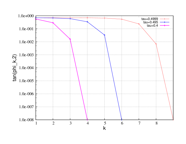
Figure 2: The tangents $\tan\varphi_{k,2}$ from Eq. (29) is plotted for $\tau\in\{0.4,\,0.495,\,0.4999\}$.

5.2 Example 2

Most algorithms in ab initio electronic structure theory compute quantities in terms of one- and two-electron integrals. In [1] we considered the low-rank approximation of the two-electron integrals. In order to illustrate the convergence of the ALS method on an example of practical interest, we use the two-electron integrals of the so called AO basis for the CH₄ molecule. We refer the reader to [1] for a detailed description of our example. The ALS method converges here Q-linearly, see Figure 3.

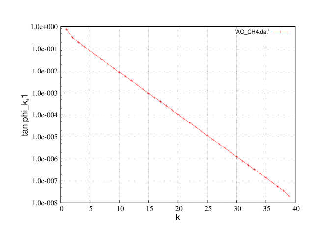
Figure 3: The approximation of two-electron integrals for methane is considered. The tangents of the angle between the current iteration point and the limit point with respect to the iteration number is shown.

5.3 Example 3

We consider the tensor

$$b_{\lambda}=\bigotimes_{\mu=1}^{3}p+\lambda\left(p\otimes q\otimes q+q\otimes p\otimes q+q\otimes q\otimes p\right)$$

from Remark 4.23. The vectors $p$ and $q$ are arbitrarily generated orthogonal vectors with norm $1$. The values of $\tan(\varphi_{1,k})$ are plotted, where $\varphi_{1,k}$ is the angle between $p_{1}^{k}$ and the limit point $p$. For the case $\lambda=0.5$ the convergence is sublinearly, whereas for $\lambda<0.5$ it is Q-linearly. According to Theorem 4.21 and [13], the rate of convergence for an ALS micro-step is given by

$$q_{\lambda}=\limsup_{k\rightarrow\infty}\left|\frac{q_{k,1}^{(s,\lambda)}}{q_{k,1}^{(c,\lambda)}}\right|=\frac{\lambda}{2}\left(3\lambda+\lambda^{2}+\sqrt{(3\lambda+\lambda^{2})^{2}+4\lambda}\right).$$

For $\lambda=0.46$, we have for the convergence rate $q_{0.46}=0.847$. In Figure 6 the ratio $\frac{\tan(\varphi_{1,k+1})}{\tan(\varphi_{1,k})}$ is plotted. The ratio $\frac{\tan(\varphi_{1,k+1})}{\tan(\varphi_{1,k})}$ perfectly matches to $q_{0.46}=0.847$. This plot shows on an example the precise analytical description of the convergence rate.

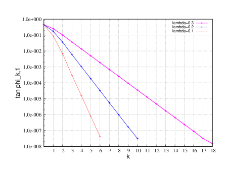
(a) The tangents $\tan\varphi_{k,1}$ for $\lambda\in\{0.1,\,0.2,\,0.3\}$.

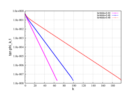
(b) The tangents $\tan\varphi_{k,1}$ for $\lambda\in\{0.44,\,0.46,\,0.48\}$.

Figure 4: The approximation of $b_{\lambda}$ from Remark 4.23 is considered. The tangents of the angle between the current iteration point and the limit point with respect to the iteration number is plotted. For $\lambda<0.5$ the sequence converges Q-linearly with a convergence rate $q_{\lambda}=\frac{\lambda}{2}\left(3\lambda+\lambda^{2}+\sqrt{(3\lambda+\lambda^{2})^{2}+4\lambda}\right)<1$.

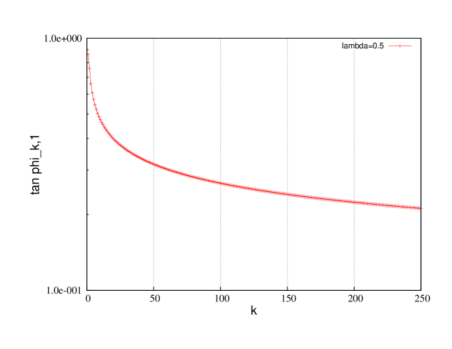
Figure 5: The approximation of $b_{\lambda}$ from Remark 4.23 is considered. The tangents of the angle between the current iteration point and the limit point with respect to the iteration number is plotted. For $\lambda=0.5$, we have sublinear convergence since $q_{0.5}=1$.

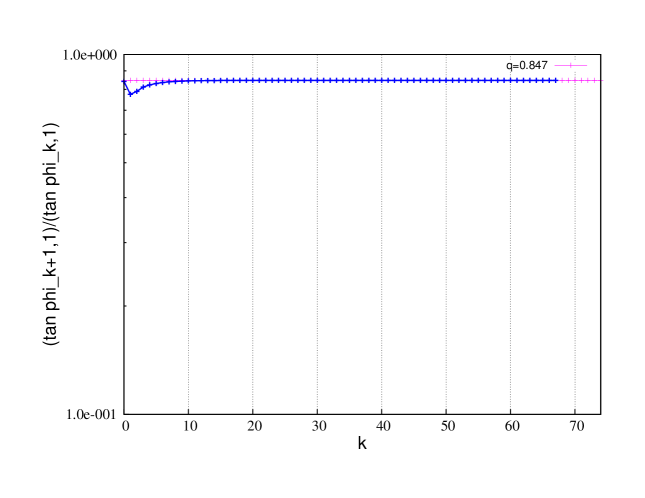
Figure 6: The ratio $\frac{\tan(\varphi_{1,k+1})}{\tan(\varphi_{1,k})}$ is plotted for $\lambda=0.46$. The rate of convergence from Theorem 4.21 is for this example equal to $0.847$. The plot illustrates that the description of the convergence rate is accurate and sharp.

References

- [1] U. Benedikt, A. Auer, M. Espig, and W. Hackbusch. Tensor decomposition in post-hartree–fock methods. i. two-electron integrals and mp2. The Journal of Chemical Physics, 134(5):–, 2011.
- [2] G. Beylkin and M. J. Mohlenkamp. Numerical operator calculus in higher dimensions. Proceedings of the National Academy of Sciences, 99(16):10246–10251, 2002.
- [3] G. Beylkin and M. J. Mohlenkamp. Algorithms for numerical analysis in high dimensions. SIAM Journal on Scientific Computing, 26(6):2133–2159, 2005.
- [4] C. Brezinski. Projection methods for systems of equations. Studies in computational mathematics. Elsevier Science, 1997.
- [5] V. de Silva and L.-H. Lim. Tensor rank and the ill-posedness of the best low-rank approximation problem. SIAM. J. Matrix Anal. and Appl., 30:1084–1127, 2008.
- [6] Alireza Doostan, AbdoulAhad Validi, and Gianluca Iaccarino. Non-intrusive low-rank separated approximation of high-dimensional stochastic models. Comput. Methods Appl. Mech. Engrg., 263:42–55, 2013.
- [7] M. Espig. Effiziente Bestapproximation mittels Summen von Elementartensoren in hohen Dimensionen. PhD thesis, Universität Leipzig, 2008.
- [8] M. Espig, L. Grasedyck, and W. Hackbusch. Black box low tensor rank approximation using fibre-crosses. Constructive approximation, 2009.
- [9] M. Espig and W. Hackbusch. A regularized newton method for the efficient approximation of tensors represented in the canonical tensor format. Num. Math., 2012.
- [10] M. Espig, W. Hackbusch, S. Handschuh, and R. Schneider. Optimization problems in contracted tensor networks. Computing and Visualization in Science, 14(6):271–285, 2011.
- [11] M. Espig, W. Hackbusch, A. Litvinenko, H. G. Matthies, and E. Zander. Efficient analysis of high dimensional data in tensor formats. accepted for Springer Lecture Note series for Computational Science and Engineering, 2011.
- [12] M. Espig, W. Hackbusch, T. Rohwedder, and R. Schneider. Variational calculus with sums of elementary tensors of fixed rank. Numerische Mathematik, 2012.
- [13] M. Espig and A. Khachatryan. Convergence of alternating least squares optimisation for rank-one approximation to high order tensors. Preprint: https://www.igpm.rwth-aachen.de/forschung/preprints/412, 2014.
- [14] Mike Espig, Wolfgang Hackbusch, Alexander Litvinenko, Hermann G. Matthies, and Philipp Wähnert. Efficient low-rank approximation of the stochastic Galerkin matrix in tensor formats. Computers & Mathematics with Applications, 2012.
- [15] L. Grasedyck. Hierarchical singular value decomposition of tensors. SIAM J. Matrix Analysis Applications, 31(4):2029–2054, 2010.
- [16] W. Hackbusch. Tensor Spaces and Numerical Tensor Calculus. Springer, 2012.
- [17] W. Hackbusch and S. Kühn. A new scheme for the tensor representation. The journal of Fourier analysis and applications, 5(15):706–722, 2009.
- [18] S. Holtz, T. Rohwedder, and R. Schneider. The alternating linear scheme for tensor optimization in the tensor train format. SIAM J. Sci. Comput., 34(2):683–713, March 2012.
- [19] H. Keller. On the solution of singular and semidefinite linear systems by iteration. Journal of the Society for Industrial and Applied Mathematics Series B Numerical Analysis, 2(2):281–290, 1965.
- [20] B. N. Khoromskij and C. Schwab. Tensor-structured galerkin approximation of parametric and stochastic elliptic pdes. SIAM J. Sci. Comput., 33(1):364–385, February 2011.
- [21] T. G. Kolda and B. W. Bader. Tensor decompositions and applications. SIAM REVIEW, 51(3):455–500, 2009.
- [22] Joseph M. Landsburg, Yang Qi, and Ke Ye. On the geometry of tensor network states. Quantum Information and Computation, 12(3-4):346–354, 2012.
- [23] Young-Ju Lee, Jinbiao Wu, Jinchao Xu, and Ludmil Zikatanov. On the convergence of iterative methods for semidefinite linear systems. SIAM J. Matrix Anal. Appl., 28(3):634–641, August 2006.
- [24] H. G. Matthies and E. Zander. Solving stochastic systems with low-rank tensor compression. 436(10):3819–3838, May 2012.
- [25] M. J. Mohlenkamp. Musings on multilinear fitting. Linear Algebra Appl., 438(2):834–852, 2013.
- [26] Anthony Nouy. A generalized spectral decomposition technique to solve a class of linear stochastic partial differential equations. Comput. Methods Appl. Mech. Engrg., 196(45-48):4521–4537, 2007.
- [27] Anthony Nouy. Proper generalized decompositions and separated representations for the numerical solution of high dimensional stochastic problems. Arch. Comput. Methods Eng., 17(4):403–434, 2010.
- [28] J. M. Ortega and W. C. Rheinboldt. Iterative Solution of Nonlinear Equations in Several Variables. Society for Industrial Mathematics, 1970.
- [29] I. V. Oseledets. Dmrg approach to fast linear algebra in the tt-format. Comput. Meth. in Appl. Math., 11(3):382–393, 2011.
- [30] I. V. Oseledets. Tensor-train decomposition. SIAM J. Scientific Computing, 33(5):2295–2317, 2011.
- [31] I. V. Oseledets and S. V. Dolgov. Solution of linear systems and matrix inversion in the tt-format. SIAM J. Scientific Computing, 34(5), 2012.
- [32] I. V. Oseledets and E. Tyrtyshnikov. Breaking the curse of dimensionality, or how to use svd in many dimensions. SIAM J. Scientific Computing, 31(5):3744–3759, 2009.
- [33] T. Rohwedder and A. Uschmajew. On local convergence of alternating schemes for optimization of convex problems in the tensor train format. SIAM Journal on Numerical Analysis, 51(2):1134–1162, 2013.
- [34] Y. Saad. Iterative Methods for Sparse Linear Systems. Society for Industrial and Applied Mathematics, 2000.
- [35] A. Szabó and N.S. Ostlund. Modern Quantum Chemistry: Introduction to Advanced Electronic Structure Theory. Dover Books on Chemistry Series. Dover Publications, 1996.
- [36] A. Uschmajew. Local convergence of the alternating least squares algorithm for canonical tensor approximation. SIAM Journal on Matrix Analysis and Applications, 33(2):639–652, 2012.