Domains of analyticity of Lindstedt expansions of KAM tori in dissipative perturbations of Hamiltonian systems

Abstract.

Many problems in Physics are described by dynamical systems that are conformally symplectic (e.g., mechanical systems with a friction proportional to the velocity, variational problems with a small discount or thermostated systems). Conformally symplectic systems are characterized by the property that they transform a symplectic form into a multiple of itself. The limit of small dissipation, which is the object of the present study, is particularly interesting.

We provide all details for maps, but we present also the (somewhat minor) modifications needed to obtain a direct proof for the case of differential equations. We consider a family of conformally symplectic maps $f_{\mu,\varepsilon}$ defined on a $2d$-dimensional symplectic manifold ${\mathcal{M}}$ with exact symplectic form $\Omega$; we assume that $f_{\mu,\varepsilon}$ satisfies $f_{\mu,\varepsilon}^{*}\Omega=\lambda(\varepsilon)\Omega$. We assume that the family depends on a $d$-dimensional parameter $\mu$ (called drift) and also on a small scalar parameter $\varepsilon$. Furthermore, we assume that the conformal factor $\lambda$ depends on $\varepsilon$, in such a way that for $\varepsilon=0$ we have $\lambda(0)=1$ (the symplectic case). We also assume that $\lambda(\varepsilon)=1+\alpha\varepsilon^{a}+O(|\varepsilon|^{a+1})$, where $a\in{\mathbb{Z}}_{+}$, $\alpha\in{\mathbb{C}}\backslash\{0\}$.

We study the domains of analyticity in $\varepsilon$ near $\varepsilon=0$ of perturbative expansions (Lindstedt series) of the parameterization of the quasi–periodic orbits of frequency $\omega$ (assumed to be Diophantine) and of the parameter $\mu$. Notice that this is a singular perturbation, since any friction (no matter how small) reduces the set of quasi-periodic solutions in the system. We prove that the Lindstedt series are analytic in a domain in the complex $\varepsilon$ plane, which is obtained by taking from a ball centered at zero a sequence of smaller balls with center along smooth lines going through the origin. The radii of the excluded balls decrease faster than any power of the distance of the center to the origin. We state also a conjecture on the optimality of our results.

The proof is based on the following procedure. To find a quasi-periodic solution, one solves an invariance equation for the embedding of the torus, depending on the parameters of the family. Assuming that the frequency of the torus satisfies a Diophantine condition, under mild non–degeneracy assumptions, using a Lindstedt procedure we construct an approximate solution to all orders of the invariance equation describing the KAM torus; the zeroth order Lindstedt series is provided by the solution of the invariance equation of the symplectic case. Starting from such approximate solution, we implement an a-posteriori KAM theorem to get the true solution of the invariance equation, and we show that the procedure converges. This allows also the study of monogenic and Withney extensions.

1. Introduction

Many problems of physical interest are described by models given by Hamiltonian systems with a small dissipation.

Some important particular cases of systems with dissipation are the following:

• Hamiltonian systems with a dissipation proportional to the velocity describing, e.g., problems of Celestial Mechanics – see [Cel10];

• Euler-Lagrange equations of exponentially discounted systems – very natural in finance, when inflation is present and one wants to minimize the cost in present money – see [Ben88, ISM11, DFIZ14];

• Gaussian thermostats - see [DM06, WL98].

In the examples above, it was discovered that there is a nice geometric structure, namely that the natural symplectic form is transformed into a multiple of itself by the dynamics. Systems that have this geometric property are referred to as conformally symplectic. Besides their applications to physical problems, conformally symplectic systems were considered on their own in differential geometry ([Ban02, Agr10]).

This geometric structure has important consequences for the dynamics (see Section 1.1). Notably for our purposes, there is a KAM theory with an a-posteriori format and a systematic way of obtaining perturbative expansions, see [CCdlL13c].

In this paper, we study the analyticity properties of the parameterization of the quasi-periodic solutions and of the drift parameter of conformally symplectic systems. Perturbative expansions to all orders are easy to obtain and have been considered for a long time (as a matter of fact, we will develop also very efficient methods of computation of perturbative expansions).

Notice that adding a dissipation to a Hamiltonian system is a very singular perturbation. We expect that a Hamiltonian system admits quasi-periodic solutions with many frequencies. On the other hand, a system with a positive dissipation – even if extremely small – leads to the creation of attractors which have few – or even none ! – quasi-periodic solutions. This is why one has to consider external parameters such as the drift.

Hence, we do not expect that the asymptotic expansions converge and therefore the parameterization functions will not be analytic in $\varepsilon$ in any ball centered at the origin. A common strategy in the literature of singularly perturbed problems has been to device asymptotic expansions and show that, even if they do not converge, they can be resummed. See [Bal94, Har49, BGM96] for general mathematical treatments and [LGZJ90, AFC90, KSF01] for surveys of applications of resummation techniques to concrete problems in Physics. For singular perturbation expansions in dynamical problems similar to the ones in this paper, there have been quite a number of studies (see, e.g., [GM96, GG02, GBD06, Gen10, GG05, CFG13, CFG14]). In this work, we follow a different approach from resummation. By using an a-posteriori theorem, we show (see Theorem 12) that the parameterization and the drift are analytic in $\varepsilon$ in a domain (called ${\mathcal{G}}$ and defined precisely in (2.5)) obtained by removing from a ball centered at the origin a sequence of (much smaller) balls with centers in smooth curves going through the origin. The radii of these balls decrease very fast (faster than any power of the size of the distance to the center of the excluded ball) as the centers of the excluded balls go to zero. Hence, even if the domain does not contain a ball centered at the origin, it is hard to distinguish it from a full ball (see Figure 1).

We emphasize that we only prove rigorously that ${\mathcal{G}}$ is a lower bound for the analyticity domain. The results can be improved in many ways (see Section 10.4). On the other hand, in Section 9 we conjecture that the domain ${\mathcal{G}}$ is essentially optimal in the sense that for a generic system none of the excluded balls can be filled completely (we present heuristic arguments for the conjecture and a proof of a weaker result (Proposition 23) that shows that, given any ball, one can find systems where the analyticity domain does not cover the ball). We note that the domains we find have only sectors centered at the origin with very small apertures, say $\pi/a$, where $a$ is the leading exponent in the change of the conformal factor.

The conjecture that there are no sectors of analyticity with aperture bigger than $\pi/a$ has consequences for resummability methods and asymptotic expansions, since uniqueness of the function given by the expansion and Borel summation often requires that there are sectors of angular aperture of about $\pi$, see [Sok80] (the well known Cauchy functions $\exp(-1/\varepsilon^{2})$ provide examples of non-trivial functions with trivial asymptotic expansions in domains of angular aperture less than $\pi$).

We also recall that, since the parameterization is a function, the notion of analytic functions taking values on parameterizations requires that we specify a Banach space in which the parameterization lies. This is done in Section  2. We anticipate that these spaces for the parameterization are spaces of analytic functions from a complex extension of the torus to the phase space.

The method of proof of this paper is to formulate a functional equation for the parameterization of the torus and the drift expressing that the torus is invariant for the map with the adjusted parameters. First, we show (part A of Theorem 14) that it is possible to find a solution of the invariance equation in the sense of formal power series (this is a very standard order by order perturbation expansion, but in Section 10 we also construct fast algorithms that double the order in each step). By truncating appropriately this formal power series, we obtain functions that solve the invariance equation very approximately. These approximate solutions are taken as the initial points of an iterative procedure which is shown to converge by an a-posteriori theorem (see Theorem 14), which is very similar to Theorem 20 in [CCdlL13c]. The domain ${\mathcal{G}}$ is obtained by examining carefully the process, and the quantitative and explicit conditions of Theorem 14. Notice that for the applications in this paper, it is essential that Theorem 14 is formulated in an a-posteriori format (we can start the iteration of an approximate solution even if the problem is not close to integrable and also we can obtain estimates on the distance from the initial data to the solution by the error of the initial approximation).

Methods similar to those described above (using a formal power series as a jumping off point of an a-posteriori method) were used in [JdlLZ99]. One can also mention [CCdlL13b, CCCdlL15] which deal with dissipative systems, although in the two latter papers the iterative method is not a Newton’s method, but rather a contraction argument (taking advantage of the fact that the dissipation is very strong). The method is very well suited for the study of monogenic properties and Whitney extensions, which we study in Section 10.

We expect that the phenomena uncovered here also hold in several other problems.

1.1. Conformally symplectic systems

As mentioned above, there are many physical problems that lead to the study of conformally symplectic systems and, in particular, to the study of singular series.

One simple but very useful remark for conformally symplectic systems is that quasi-periodic solutions with enough frequencies satisfy the so-called automatic reducibility: in a neighborhood of an (approximately) invariant torus, one can find a system of coordinates in which the linearization becomes (approximately) constant coefficients. Automatic reducibility happens irrespective of whether the system is close to integrable or not (see [CCdlL13c]). Automatic reducibility allows one to develop a KAM theory ([CCdlL13c]), leading also to efficient and accurate algorithms.

In [CCdlL13c] one can find a numerically accessible method to compute the breakdown threshold extending the arguments of [CdlL10b]. This criterion for breakdown, based on the study of the growth of Sobolev norms, is shown to converge to the right value of the threshold; indeed, the accuracy of the computed breakdown in actual computers is only limited by the available memory, precision and computational time.

A numerical implementation in actual computers was done in [CC10], which includes comparisons with other methods. Another property of KAM tori in conformally symplectic systems is that the breakdown of the invariant circles happens due to a bundle collapse scenario in which hyperbolicity is lost because the stable bundle becomes close to the tangent bundle, even if the exponents remain bounded away (see [CF12] for a numerical implementation and a presentation of empirical results, including scaling relations for the breakdown).

We also mention that the Greene’s criterion for the breakdown of invariant circles has been extended to conformally symplectic systems and given a partial justification (see [CCFdlL14]).

It is known that KAM theory for conformally symplectic systems requires adjusting parameters ([CCdlL13c]) and moreover (see [CCdlL13a]) that Birkhoff invariants near a Lagrangian invariant torus with a dynamics conjugated to a rotation disappear (i.e., given a Lagrangian invariant torus with a dynamics conjugated to a rotation, there is an analytic and symplectic change of variables defined in a neighborhood of the torus, that conjugates the dynamics to a rotation in the angles and a multiplication by a constant in the actions).

The papers [SL12, SL15] develop a Kolmogorov theory based on transformation theory for quasi-periodic solutions in quasi-integrable conformally symplectic systems and implement it numerically. The paper [CC09] develops an a-posteriori KAM theory for the spin-orbit problem (a two degrees of freedom conformally symplectic system).

1.2. Description of the set up

We will consider analytic families of mappings or flows with a small parameter $\varepsilon$ and having also internal parameters $\mu$. That is, given an analytic symplectic manifold ${\mathcal{M}}$ of dimension $2d$ with exact symplectic form $\Omega$, we will consider families of mappings $f_{\mu,\varepsilon}:{\mathcal{M}}\rightarrow{\mathcal{M}}$ satisfying:

$$f_{\mu,\varepsilon}^{*}\Omega=\lambda(\varepsilon)\Omega\ ,\qquad\lambda(0)=1\,$$ (1.1)

or families of flows ${\mathcal{F}}_{\mu,\varepsilon}$ such that:

$$L_{{\mathcal{F}}_{\mu,\varepsilon}}\Omega=\chi(\varepsilon)\Omega\ ,\qquad\chi(0)=0\ ,$$ (1.2)

where $\lambda=\lambda(\varepsilon)$, $\chi=\chi(\varepsilon)$ are the conformal factors for maps and flows, respectively, the star in (1.1) denotes the pull-back, $L_{{\mathcal{F}}_{\mu,\varepsilon}}$ in (1.2) is the Lie derivative. We will refer to $\lambda(\varepsilon)$, $\chi(\varepsilon)$ as the dissipation.

Since we will discuss analyticity, all the parameters will be taken to be complex. In applications the parameters are often real and then the values of the functions are real. It will happen that all the calculations we perform respect the properties that real arguments of the function lead to real results.

In formula (1.1), $\varepsilon$ is a small parameter that controls the dissipation. The parameters $\mu\in{\mathbb{C}}^{d}$ are some intrinsic parameters of the model that are called the drift in some papers. Of course, the case when $\lambda=1$ (respectively, $\chi=0$) corresponds to the mapping $f_{\mu,\varepsilon}$ (respectively, the flow ${\mathcal{F}}_{\mu,\varepsilon}$) being symplectic.

Note that the interpretation of (1.1) or (1.2) is that the mapping or the flow transforms the symplectic form into a multiple (could be a complex multiple for complex $\varepsilon$) of itself. We assume that the conformal factor is of the form

$$\lambda(\varepsilon)=1+\alpha\varepsilon^{a}+O(|\varepsilon|^{a+1})\ ,$$

where $a\in{\mathbb{Z}}_{+}$, $\alpha\in{\mathbb{C}}\backslash\{0\}$ (in many applications $\alpha\in{\mathbb{R}}\backslash\{0\}$, so as to preserve the property that real arguments lead to real variables).

We will fix $\omega$ within the set of Diophantine vectors (see Definition 3 for the standard definition for maps and Appendix A for the standard definition for flows). We will be interested in studying the domain of complex values of $\varepsilon$ for which we can continue a KAM torus invariant for the symplectic system.

Of course, we will assume several non-degeneracy conditions (similar to the twist condition) to prove the existence of KAM tori. These non-degeneracy conditions can be verified by performing some calculations on the approximate solution.

Note, that we will not assume that the Hamiltonian system is integrable or nearly-integrable, but only that it has a KAM torus of frequency $\omega$. In particular, the results apply to perturbations of islands generated by resonances at higher values of the perturbation ([Dua94], [Dua99]).

For simplicity we will describe in detail the case of maps, while flows are discussed in Appendix A.

The way we seek invariant tori of mappings is to try to find an embedding $K_{\varepsilon}:{\mathbb{T}}^{d}\rightarrow{\mathcal{M}}$ and a parameter vector $\mu_{\varepsilon}\in{\mathbb{C}}^{d}$ in such a way that

$$f_{\mu_{\varepsilon},\varepsilon}\circ K_{\varepsilon}=K_{\varepsilon}\circ T_{\omega}\ ,$$ (1.3)

where $T_{\omega}$ is the shift map defined by $\omega$, $T_{\omega}(\theta)=\theta+\omega$. We will fix $\omega$ to be Diophantine (see Section 2.1). Of course, the equation (1.3) will have to be supplemented by some normalization conditions, which ensure that the solutions are locally unique. We refer to [CdlL09, CdlL10a, dlLR91, CF12] for a method to find invariant curves that solve the invariance equation (1.3) numerically.

Our main result, Theorem 12, shows that, if there is a solution of (1.3) for $\varepsilon=0$ (the symplectic case), which satisfies some mild non-degeneracy conditions, we can find $K_{\varepsilon}$ and $\mu_{\varepsilon}$ defined for a set ${\mathcal{G}}$ of $\varepsilon$. The functions $K_{\varepsilon}$ and the vectors $\mu_{\varepsilon}$ are analytic in $\varepsilon$ when $\varepsilon$ ranges in the interior of the sets which are described in Section 2.2.1. They also extend continuously to the boundary of ${\mathcal{G}}$. We anticipate that the sets ${\mathcal{G}}$ do not include any ball centered at the origin in the complex plane, even if they contain the origin in their closure. On the other hand, the sets ${\mathcal{G}}$ fail to include a ball centered at the origin by very little. As we will see, the domains are obtained by taking from the ball centered at the origin a sequence of smaller balls centered along smooth lines going through the origin and with radii decreasing faster than any power of the distance of the center to the origin (see Section 2.2.1 and Figure 1).

Similar analyticity domains appeared in [JdlLZ99], where the authors used a strategy close to ours in considering the domains of analyticity of resonant tori in near-integrable systems (see also [GG05, GGG06, CGGG07] for results based on resummation of series for the same problem as [JdlLZ99]). The paper [JdlLZ99] also obtained other geometric results such as the monodromy of the stable and unstable bundles, which are not present in other treatments.

We note that the domains we obtain here have several cuts and that the analyticity domains do not contain sectors centered at the origin with aperture bigger than $\pi/a$. Hence, one cannot use only general complex analysis methods ([Har49, Bal94, Sok80]) to deal with the asymptotic series, as these methods do not guarantee that there is only a function with the same asymptotic expansion ([PL08, SZ65]). On the other hand, it is a byproduct of our analysis that the expansions of solutions of the equations using the Lindstedt procedure are indeed unique. In Section 10.5 we also discuss $C^{\infty}$-Whitney properties of the solution.

The argument we present to prove our results has two ingredients:

• An a-posteriori KAM theorem (Theorem 14) for conformally symplectic systems with complex parameters, which shows that if there is an approximate solution of the invariance equation (1.3), then there is a true solution nearby.

  Theorem 14 is a very quantitative statement on when a solution is approximate enough to be the starting point of an iterative algorithm which converges. The main condition of Theorem 14 is that the initial error is small enough. The precise smallness condition depends mainly on the number theoretic properties of the complex number $\lambda$ – the conformal factor – with respect to the frequency $\omega$. The smallness condition depends also on the Diophantine properties of $\omega$ and on some non-degeneracy conditions of the map. The Theorem 14 is a small modification of Theorem 20 in [CCdlL13c].

• An algorithm to produce a perturbative series expansion that provides approximate solutions to all orders in $\varepsilon$, see part A of Theorem 12.

  This algorithm is quite a standard procedure, which goes back at least to [Poi87] and is based on earlier literature.

  In our case, taking advantage of the fact that the maps are conformally symplectic (and, hence, automatically reducible) we can improve the classical results in several directions: In Section 10.2 we present a quadratic algorithm to compute the Lindstedt series, which is much faster and which could replace part A of Theorem 12. Indeed, the quadratic procedure in Section 10.2 gives an alternative proof of all of Theorem 12. We also note that using the automatic reducibility we can develop these series starting at any invariant torus. This leads to improvements on the domain of analyticity that are discussed in Section 10.4 as well as to Whitney regularity in the boundary.

Theorem 12 is proved by showing that an iterative procedure (which is explicitly described in Algorithm 16 and which is a very practical numerical algorithm implemented in [CC10, CF12]) converges if the initial error is small. We point out that, if we start the iterative procedure not on one parameterization and a drift, but on an analytic family of parameterizations and drifts indexed by a variable $\varepsilon$, then the result will also be an analytic family in $\varepsilon$ (the iterative procedure – see Algorithm 16 – consists in applying algebraic operations, taking derivatives and solving cohomology equations with constant coefficients; all these elementary steps preserve the analytic dependence on parameters). We also point out that the convergence will be uniform in a domain of $\varepsilon$, if all the non-degeneracy conditions and the initial error are uniform.

Hence, if we start the iterative procedure with a function analytic in an open set (respectively, continuous in a closed set) of $\varepsilon$ (such as that produced by part A in Theorem 12), then we obtain that the limit is analytic (respectively, continuous) in $\varepsilon$ in the domain where the convergence is uniform.

Since, furthermore, we have local uniqueness of the normalized solutions of the invariance equation that satisfy a normalization condition, we are sure that the solutions obtained in two open sets agree on the overlap, and hence we can use arguments based on analytic continuation.

For simplicity, we will present the proof for maps and we provide the changes needed to obtain the result for flows in Appendix A.

This paper is organized as follows. In Section 2, we collect some of the standard definitions; in Section 2.1 we provide some definitions on Diophantine properties, while in Section 2.2 we present the geometry of several sets where the conformal factors satisfy Diophantine conditions. In Section 3 we present the invariance equation and the normalization conditions we impose to obtain local uniqueness.

In Section 4 we state Theorem 12, the main result of this paper.

In Section 5 we present Theorem 14, which is the a-posteriori theorem alluded in $(i)$ above. Such a theorem is the first ingredient of the main result. The proof of Theorem 14 is very similar to the proof of Theorem 20 in [CCdlL13c] and we just outline the (rather minor) differences. The existence of the Lindstedt series is discussed in Section 6. In contrast to the procedure using Lindstedt series ([CCdlL13c]), the present treatment allows one that the conformal factor depends on $\varepsilon$. This provides the proof of the first part of Theorem 12, while the second part is proved in Section 7. In Section 8 we study some geometric properties of the set. In Section 9 we include a conjecture on the optimality of the results described in this work. In Section 10 we present several results: we show that the Lindstedt series expansions can be obtained around any point; we present a relation with the theory of monogenic functions and establish that the embedding function and the drift are Whitney differentiable in the domain; we provide a quadratic method for the computation of the Lindstedt series, leading also to Part B of Theorem 12; we present a discussion on the improvement of the domain of analyticity. The extension to the case of flows is provided in Appendix A.

Remark 1.

In many estimates in this paper, we can obtain that the domains satisfy upper bounds less or equal than $C_{N}|\varepsilon|^{N}$ for all $N$ and for some constant $C_{N}$. Clearly, since the bounds are true for all $N$, one can get an upper bound less or equal than $\inf_{N}C_{N}|\varepsilon|^{N}\equiv\Gamma(\varepsilon)$. The function $\Gamma$ will, of course, go to zero faster than any power.

If one had explicit forms for $C_{N}$, it would be possible to obtain explicit forms for $\Gamma$. In many problems similar to the ones we are considering, one obtains factorial bounds like $C_{N}=AN^{aN}$ for some constants $a$ and $A$. In such a case, one obtains that $\Gamma(\varepsilon)=\exp(-C^{\prime}|\varepsilon|^{-1/a})$ for some constant $C^{\prime}$. We conjecture that the sizes of the balls to be excluded in the present paper satisfy the factorial bounds.

2. Some definitions

In this Section, we collect some definitions on spaces, Diophantine properties and we set the notation. Most of the definitions in this section are standard. One non-standard definition that will play an important role is the Diophantine property of complex numbers with respect to a Diophantine frequency (see Definition 4).

Given $\rho>0$ we define the complex extension of the $d$–dimensional torus as

$${\mathbb{T}}^{d}_{\rho}=\{z\in{\mathbb{C}}^{d}/{\mathbb{Z}}^{d}\,:\ {\rm Re}(z_{j})\in{\mathbb{T}}\ ,\quad|\operatorname{Im}(z_{j})|\leq\rho\ ,\quad j=1,...,d\}\ .$$

We define ${\mathcal{A}}_{\rho}$ to be the vector space of functions analytic in Int(${\mathbb{T}}^{d}_{\rho}$) and which extend continuously to the boundary of ${\mathbb{T}}^{d}_{\rho}$.

We endow ${\mathcal{A}}_{\rho}$ with the supremum norm

$$||f||_{\rho}=\sup_{\theta\in{\mathbb{T}}^{d}_{\rho}}|f(\theta)|\ .$$ (2.1)

The norm (2.1) makes the space ${\mathcal{A}}_{\rho}$ into a Banach space, indeed a Banach algebra under multiplication. An important closed subspace of ${\mathcal{A}}_{\rho}$ is the set of functions which take real values for real arguments.

Analogous definitions are made for analytic functions on ${\mathbb{T}}^{d}_{\rho}$ taking values in vectors or in matrices and, of course, the multiplicative properties of norms of vectors and matrices lift to supremum norms of functions taking values in vectors or matrices.

We also note that we can define analytic functions of $\varepsilon\in{\mathbb{C}}$ taking values in ${\mathcal{A}}_{\rho}$. Following standard definitions, we say that an ${\mathcal{A}}_{\rho}$-valued function $K$ is analytic in an open domain ${\mathcal{D}}\subset{\mathbb{C}}$ when, for any $\varepsilon_{0}\in{\mathcal{D}}$, we can represent for all $|\varepsilon-\varepsilon_{0}|$ sufficiently small, $K_{\varepsilon}=\sum_{n=0}^{\infty}K_{n}(\varepsilon-\varepsilon_{0})^{n}$, where the convergence of the infinite sum happens in ${\mathcal{A}}_{\rho}$. Note that, with this definition, it is clear that an ${\mathcal{A}}_{\rho}$-valued analytic function is also an ${\mathcal{A}}_{\rho^{\prime}}$-valued analytic function for $\rho^{\prime}\leq\rho$.

It is remarkable that there are many other definitions that are apparently weaker than the definition above, but which turn out to be equivalent (see [Hil48, Chapter III]). In our case, the $K$ will be analytic functions from ${\mathcal{G}}$ to some ${\mathcal{A}}_{\rho}$. In principle, the domain ${\mathcal{G}}$ could depend on $\rho$, but we will not include it in the notation.

We note that we are only obtaining lower bounds of the domain of analyticity. The method of proof leads to estimates for different $\rho$’s, which are proved by selecting a different constant. Hence, the statements that are valid for all Diophantine constants in a range are also valid for all the values of $\rho$ in a range.

We recall the classical Cauchy inequalities for derivatives and for Fourier coefficients (see, e.g., [SZ65, Rüs75]).

Proposition 2.

For any $0<\delta<\rho$ and for any function $K\in{\mathcal{A}}_{\rho}$, denoting by $D^{j}$ the $j$–th derivative, we have:

$$||D^{j}K||_{\rho-\delta} \leq C_{j}\delta^{-j}||K||_{\rho}\ ,$$

$$|\widehat{K}_{k}| \leq ||K||_{\rho}\ e^{-2\pi|k|\rho}\ ,$$

for some constants $C_{j}$, where $\widehat{K}_{k}$ denotes the $k$–th Fourier coefficient of $K$ and $|k|=|k_{1}|+...+|k_{d}|$.

2.1. Diophantine properties

In this Section we collect some definitions concerning Diophantine properties, which will be needed to bound the small divisors appearing in the solution of the invariance equation. The only non standard definition is Definition 4.

Definition 3.

Let $\omega\in{\mathbb{R}}^{d}$, $\tau\in{\mathbb{R}}_{+}$. We define the quantity $\nu(\omega;\tau)$ as

$$\nu(\omega;\tau)\equiv\sup_{k\in{\mathbb{Z}}^{d}\setminus\{0\}}|e^{2\pi ik\cdot\omega}-1|^{-1}|k|^{-\tau}\ .$$ (2.2)

In the sup above we allow $\infty$. Also, if $|e^{2\pi ik\cdot\omega}-1|=0$, we set $\nu(\omega;\tau)=\infty.$

We say that $\omega\in{\mathbb{R}}^{d}$ is Diophantine of class $\tau$ and constant $\nu(\omega;\tau)$, whenever

$$\nu(\omega;\tau)<\infty\ .$$ (2.3)

We denote by ${\mathcal{D}}_{d}(\nu,\tau)$ the set of Diophantine vectors in ${\mathbb{R}}^{d}$ of class $\tau$ and constant $\nu$.

Of course, if $\omega$ is Diophantine of class $\tau$, it will be Diophantine of class $\psi$ for all $\psi\geq\tau$. For the purposes of this paper, the value of the constant $\nu$ is more important than the exponent $\tau$, so we will consider one fixed exponent in the main theorems.

Definition 4.

Let $\lambda\in{\mathbb{C}}$, $\omega\in{\mathbb{R}}^{d}$, $\tau\in{\mathbb{R}}_{+}$. We define the quantity $\nu(\lambda;\omega,\tau)$ as

$$\nu(\lambda;\omega,\tau)\equiv\sup_{k\in{\mathbb{Z}}^{d}\setminus\{0\}}|e^{2\pi ik\cdot\omega}-\lambda|^{-1}|k|^{-\tau}\ .$$ (2.4)

Again, we allow $\infty$ in the supremum above and set $\nu(\lambda;\omega,\tau)=\infty$, if $e^{2\pi ik\cdot\omega}=\lambda$ for some $k\in{\mathbb{Z}}^{d}\backslash\{0\}$.

Remark 5.

We note that, for a fixed $\omega$, the function $\nu=\nu(\lambda;\omega,\tau)$ is a lower semi-continuous function of $\lambda$, since it is the supremum of continuous functions.

Remark 6.

If $\nu(\lambda;\omega,\tau)<\infty$, then for all $\psi\geq\tau$, we have $\nu(\lambda;\omega,\psi)<\infty$.

Note that the definition of $\nu(\lambda;\omega,\tau)$ does not require that $\omega$ is Diophantine of exponent $\tau$.

Remark 7.

No matter what $\omega$ is, if $|\lambda|\neq 1$, then from the inequality

$$|e^{2\pi ik\cdot\omega}-\lambda||k|^{\tau}\geq|e^{2\pi ik\cdot\omega}-\lambda|\geq\Big{|}|e^{2\pi ik\cdot\omega}|-|\lambda|\Big{|}=\Big{|}1-|\lambda|\Big{|}\ ,$$

one obtains that

$$\nu(\lambda;\omega,\tau)\leq|1-|\lambda||^{-1}<\infty$$

for any $\tau$.

As a consequence of the above remark, the only case that needs to be studied in detail is when $|\lambda|=1$, in which case it could be that $\nu(\lambda;\omega,\tau)=\infty$ (e.g., if $\lambda=e^{2\pi ik\cdot\omega}$ for some $k\in{\mathbb{Z}}^{d}\setminus\{0\}$ or if $\omega$ is a Liouville number).

For $\tau>d-1$ the set of real vectors which are not Diophantine of class $\tau$ has zero Lebesgue measure in ${\mathbb{R}}^{d}$. That is, the union over all $\nu>0$ of the sets of Diophantine vectors of class $\tau$ satisfying (2.3) with constant $\nu$, has full Lebesgue measure in ${\mathbb{R}}^{d}$. For any $\omega\in{\mathbb{R}}^{d}$, if $\tau>d-1$, the set of $\lambda$ for which $\nu(\lambda;\omega,\tau)<\infty$ is of full Lebesgue measure on the unit circle (see [Sch80]). When we consider complex $\omega\in{\mathbb{C}}^{d}$, the set of vectors that are not Diophantine of class $\tau$ has zero measure when $2\tau>d-1$. This shows that complex Diophantine is easier than Diophantine over the reals.

We will consider fixed the analytic function $\lambda(\varepsilon)$, which gives the conformal factor as a function of the perturbing parameter $\varepsilon$. In particular, we will assume that $\lambda(\varepsilon)$ is analytic in a neighborhood of zero and that $\lambda(0)=1$. Hence, we assume that $\lambda=\lambda(\varepsilon)$ satisfies:

H$\bf{\lambda}\qquad\qquad\qquad\qquad\qquad$ $\lambda(\varepsilon)-1=\alpha\varepsilon^{a}+O(|\varepsilon|^{a+1})$

for some $a>0$ integer, $\alpha\in{\mathbb{C}}\backslash\{0\}$.

This will be one of the assumptions of our main result stated in Theorem 12. Note that, since we are considering analytic functions, the alternative to the existence of $\alpha$ and $a$ in H$\bf{\lambda}$ is that $\lambda(\varepsilon)\equiv 1$, that is that the maps $f_{\mu,\varepsilon}$ are symplectic. Hence, given the analyticity assumption, the only content of H$\lambda$ is that the perturbations indeed change the symplectic character (as well as setting the notation for $a,\alpha$, which will play a role in the the quantitative statements).

We consider the function $\lambda(\varepsilon)$ as given in H$\lambda$.

We define the set ${\mathcal{G}}={\mathcal{G}}(A;\omega,\tau,N)$ for some $A>0$, $N\in{\mathbb{Z}}_{+}$, $\omega\in{\mathbb{R}}^{d}$ as

$${\mathcal{G}}(A;\omega,\tau,N)=\{\varepsilon\in{\mathbb{C}}:\quad\nu(\lambda(\varepsilon);\omega,\tau)|\lambda(\varepsilon)-1|^{N+1}\leq A\}\ .$$ (2.5)

We also introduce the notation

$${\mathcal{G}}_{r_{0}}(A;\omega,\tau,N)={\mathcal{G}}\cap\{\varepsilon\in{\mathbb{C}}:\ |\varepsilon|\leq r_{0}\}\ ;$$ (2.6)

the set ${\mathcal{G}}_{r_{0}}$ will typically be used for sufficiently small $r_{0}$.

Notice that ${\mathcal{G}}(A;\omega,\tau,N)$ is the preimage under the function $\lambda$ of the set

$$\Lambda(A;\omega,\tau,N)=\{\lambda\in{\mathbb{C}}:\quad\nu(\lambda;\omega,\tau)|\lambda-1|^{N+1}\leq A\}\ .$$ (2.7)

The motivation for introducing these sets will be discussed in Section 2.2. We anticipate that the set ${\mathcal{G}}$ is the set where the Diophantine constants of $\lambda(\varepsilon)$ are not too bad, so that a good approximation (up to a high power of $\varepsilon$) can be taken as the initial condition for an iterative procedure that converges. More detailed motivations will be presented in Section 2.2; some depiction of the sets ${\mathcal{G}}_{r_{0}}$, ${\mathcal{A}}$ is presented in Figure 1.

Since, for a fixed $\omega$, the function $\nu$ is lower semi-continuous, we note that ${\mathcal{G}}$ is a closed set. The interior of this set is non-empty and indeed, the set ${\mathcal{G}}$ is the closure of its interior. We will be studying functions defined in ${\mathcal{G}}$ taking values either in the complex or in some Banach space of functions. We will consider functions on ${\mathcal{G}}$ which are continuous in ${\mathcal{G}}$ and analytic in the interior of ${\mathcal{G}}$. We will sometimes refer to these functions as analytic in ${\mathcal{G}}$.

For obvious typographical reasons, since many of the arguments of ${\mathcal{G}},\Lambda$ will be fixed in the discussion, we will omit them: if $\omega$, $\tau$, $N$, $\lambda$ are fixed in an argument, we will just write ${\mathcal{G}}(A)$ or ${\mathcal{G}}_{r_{0}}(A)$. Of course, one could also add $\rho$ to the dependence of ${\mathcal{G}}$, but as remarked above, this is not needed.

2.2. Motivation for the role of the Diophantine constants.

In this paper, we will fix $\omega$ Diophantine and search for solutions of the functional equation (1.3), capturing the geometric idea that we have a parameterization of an invariant torus.

The solutions of the invariance equation (1.3) are obtained by an iterative method, whose step involves solving two cohomology equations of the type considered in Section 2.2.2 below (as well as algebraic and calculus operations).

One of the cohomology equations in the iterative step will involve small divisors of the form $|e^{2\pi ik\cdot\omega}-1|^{-1}$ appearing in (2.2) and the other will involve small divisors of the form $|e^{2\pi ik\cdot\omega}-\lambda|^{-1}$ appearing in (2.4). Hence, the quantitative figure of merit of the step will be the constant $\nu(\omega;\tau)\nu(\lambda;\omega,\tilde{\tau})$ for some $\tau,\tilde{\tau}\in{\mathbb{R}}_{+}$ (as well as other factors, that we will consider fixed).

Since the two cohomological equations that we are going to solve in Section 5 are different, there is no reason to impose that the exponents are equal, but, for the sake of simplicity, we will not optimize these choices and, from now on, we will just consider the case $\tilde{\tau}=\tau$.

Based on the results presented in [CCdlL13a], we will show that, if we start with an approximate solution of (1.3) and if the initial error is small enough compared with the figure of merit (the precise relation given in assumption H5 of Theorem 14), then the iterative procedure can be repeated infinitely many times and it converges to a true solution. Taking as initial condition the Lindstedt series, we will obtain convergence in the sets claimed in Theorem 12.

If we fix the frequency $\omega$ and the exponent $\tau$, the quality factor for the step, namely $\nu(\omega;\tau)\nu(\lambda;\omega,\tau)$, is a function of $\lambda$ alone. It will be important to study the places where this function is not too big and identify complex domains in the $\varepsilon$-plane where it is bounded uniformly. The values of $\lambda$ which lead to a quality factor in the iterative step, which is small enough with respect to the initial error, are those for which the procedure converges.

As indicated in hypothesis H$\lambda$, when we consider problems depending on the complex parameter $\varepsilon$, the quantity $\lambda(\varepsilon)-1$ will be approximately $\alpha\varepsilon^{a}$. The perturbation expansion to order $N$ will produce approximate solutions that satisfy the equation to order $\varepsilon^{N+1}$ (see (4.3) in Theorem 12). Hence, the sets ${\mathcal{G}}$ in (2.5) are the sets where we can start the iterative procedure with an approximate solution given by a perturbation expansion, and obtain that the iteration process converges. The sets ${\mathcal{G}}$ in (2.5) will thus be the sets where we can establish that there is a solution starting the iterative procedure from the approximate solution given by the expansion. Of course, it is possible that the set of $\varepsilon$ for which $K_{\varepsilon}$, $\mu_{\varepsilon}$ are analytic is larger than ${\mathcal{G}}$. The set ${\mathcal{G}}$ is the place where one particular method works, but we could use other methods. Indeed in Section 10.4, we will find some way to extend the domain ${\mathcal{G}}$.

We will undertake the study of the geometry of the sets ${\mathcal{G}}$ and $\Lambda$ in Section 2.2.1 and in Section 8. We anticipate that, of course, one can obtain uniform bounds for $\nu(\lambda;\omega,\tau)$ in any domain which is away from the unit circle. The function $\nu(\lambda;\omega,\tau)$ is infinite in a dense set on the unit circle, but can be bounded in domains that include the unit circle in the boundary, indeed in a full measure set in the unit disk. The geometry of these domains is rather interesting and will be discussed in the next Section.

2.2.1. Geometry of the level sets of $\nu(\lambda;\omega,\tau)$

In this Section we try to understand the sets of points described in Section 2.1. More properties will be described in Section 8.

The complement of the set $\Lambda$, say $\Lambda^{c}$, is the bad set where the bounds we use do not allow us to claim the existence of tori, but we claim that if we take as initial condition of the iterative procedure the Lindstedt polynomial of order $N$, then the measure of $\Lambda^{c}$ is small for $N$ large enough.

The set $\Lambda^{c}$ is the union of the open sets

$$\begin{split}{\mathcal{R}}_{k}&=\{\lambda\in{\mathbb{C}}\,:\ |e^{2\pi ik\cdot\omega}-\lambda|^{-1}>A|k|^{\tau}|\lambda-1|^{-(N+1)}\}\\ &=\{\lambda\in{\mathbb{C}}\,:\ |e^{2\pi ik\cdot\omega}-\lambda|<A^{-1}|k|^{-\tau}|\lambda-1|^{N+1}\}\ .\end{split}$$

Since $\lambda$ appears on both sides of the inequality defining ${\mathcal{R}}_{k}$, this is not easy to handle. On the other hand, we note that if we consider the annulus $\rho<|\lambda-1|<2\rho$, we see that the intersection of the set ${\mathcal{R}}_{k}$ with the annulus is contained in the ball ${\mathcal{B}}_{k}$ with center at $e^{2\pi ik\cdot\omega}$ and radius $CA^{-1}\rho^{N+1}|k|^{-\tau}$, for some constant $C>0$.

For each $k\in{\mathbb{Z}}^{d}\setminus\{0\}$, the area ${\mathcal{S}}_{k}$ of the ball is equal to

$${\mathcal{S}}_{k}=\pi\ C^{2}\ A^{-2}\ \rho^{2(N+1)}\ |k|^{-2\tau}\ .$$

Notice that the area of the union of the balls ${\mathcal{B}}_{k}$ is finite, provided

$$\sum_{k\in{\mathbb{Z}}^{d}\backslash\{0\}}|k|^{-2\tau}<\infty\ .$$

Indeed, we see that as we consider $\rho$ small, the excluded area decreases faster than $\rho^{2(N+1)}$, which is much smaller than the area of the annulus, which is proportional to $\rho^{2}$. Hence, we can say that $\Lambda$ has a point of density at $1$ and that the excluded balls in the $\lambda$-space decrease very fast as we approach $1$. More detailed estimates will appear later.

The above remarks can be translated to the $\varepsilon$ plane under the assumption H$\lambda$.

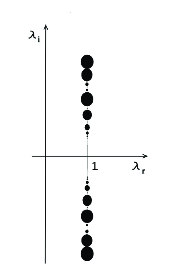
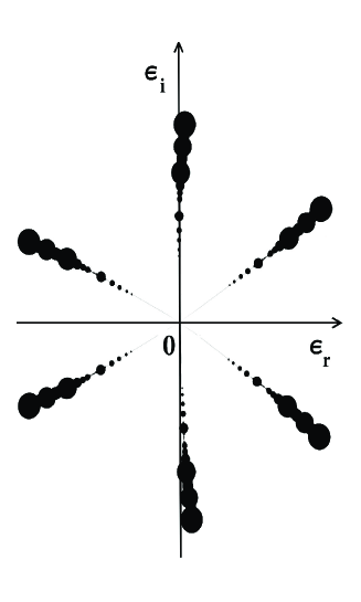
Figure 1. A representation of the sets $\Lambda$, ${\mathcal{G}}$ introduced in (2.7), (2.5); they are given by the region not covered by the black circles. The domains are obtained for $d=1$, $\tau=1$, $a=3$. The radii of the balls have been rescaled for graphical reasons. Left: in black the complement in the complex plane of the set $\Lambda$ as in (2.7); the centers of the balls lie approximately on the unit circle, which at high magnification resembles a vertical line. Right: in black the complement of the set ${\mathcal{G}}$ as in (2.5): the centers of the balls are at $|e^{2\pi ik\cdot\omega}-1|^{1\over a}$.

Figure 1 provides a representation of the circles which must be excluded from the definition of the sets introduced in (2.5) and (2.7). We remark that taking a higher exponent $N$ in (2.5), (2.7) does not alter significantly the geometry of the domains, it just makes the radius of the circles decrease faster. This fast convergence to zero of the radii makes it impossible to represent the excluded regions in a quantitatively correct way. All the circles except for a few of them will be smaller than a pixel! Nevertheless, we conjecture that these excluded circles are there, see Section 9.

2.2.2. Estimates of cohomology equations

In this Section, we will present (rather elementary) estimates on the solutions $\varphi:{\mathbb{T}}^{d}\rightarrow{\mathbb{C}}$ of twisted cohomology equations of the form:

$$\lambda\varphi(\theta)-\varphi(\theta+\omega)=\eta(\theta)\ ,$$ (2.8)

where the function $\eta:{\mathbb{T}}^{d}\rightarrow{\mathbb{C}}$, the parameter $\lambda\in{\mathbb{C}}$ and the frequency vector $\omega\in{\mathbb{R}}^{d}$ are given.

We will assume that $\omega$ is Diophantine (see Definition 3) and that $\lambda$ satisfies Definition 4 with $\nu(\lambda;\omega,\tau)<\infty$. We want to show that there exist solutions of (2.8) and that we obtain quantitative estimates on the size of these solutions in terms of the quantitative estimates of the Diophantine properties of $\lambda$. The estimates that we will obtain will be tame estimates in the sense of Nash-Moser implicit function theorems.

For subsequent applications in this paper, it will be quite important that the estimates that we obtain about $\varphi$ are rather explicit on $\nu(\lambda;\omega,\tau)$. Hence, they will hold uniformly in sets of $\lambda$ for which $\nu(\lambda;\omega,\tau)$ is uniformly bounded. The geometry of these sets was described explicitly in Section 2.2.1.

Since we will be interested in the limit $\lambda\approx 1$, it will be important that we can consider $\lambda$ ranging on domains which include $1$ as a limit point. Hence, we will insert in our hypotheses that $\omega$ is Diophantine to avoid empty statements. The following Lemma is a standard result in KAM theory; the dependence of the estimates on the exponents is not optimized as it is done for $\lambda$ real according to [Rüs75, Rüs76a]. This will lead to slightly different estimates in H5 of Theorem 14 when compared to those appearing in Theorem 20 of [CCdlL13c]; a more detailed comparison will be given later in Section 5.

Lemma 8.

Let $\omega\in{\mathcal{D}}_{d}(\nu,\tau)$, $\lambda\in{\mathbb{C}}$. Assume that $\eta\in{\mathcal{A}}_{\rho}$, $\rho>0$, is such that $\int_{{\mathbb{T}}^{d}}\eta(\theta)d\theta=0$. Then, we can find a unique $\varphi\in L^{2}({\mathbb{T}}^{d})$ solving (2.8), that also satisfies

$$\int_{{\mathbb{T}}^{d}}\varphi(\theta)d\theta=0\ .$$

Moreover, for any $0<\delta<\rho$, we have $\varphi\in{\mathcal{A}}_{\rho-\delta}$, and

$$||\varphi||_{\rho-\delta}\leq C(\tau,d)\ \nu(\lambda;\omega,\tau)\ \delta^{-\tau-d}\ ||\eta||_{\rho}$$ (2.9)

for a suitable constant $C=C(\tau,d)$.

Note that a particular case of Lemma 8 is when $\lambda=1$, which reduces to the most standard cohomology equations of KAM theory.

Proof.

The proof we present here is based on the most elementary (but possibly not optimal in the exponent for $\delta$) argument (see Remark 9 below).

We expand $\eta$ in Fourier series as $\eta(\theta)=\sum_{k\in{\mathbb{Z}}^{d}\setminus\{0\}}\hat{\eta}_{k}e^{2\pi ik\cdot\theta}$. We obtain that (2.8) is equivalent to having that for all $k\in{\mathbb{Z}}^{d}\setminus\{0\}$:

$$\lambda\hat{\varphi}_{k}-e^{2\pi ik\cdot\omega}\hat{\varphi}_{k}=\hat{\eta}_{k}\ ,$$

whose solution is

$$\hat{\varphi}_{k}=(\lambda-e^{2\pi ik\cdot\omega})^{-1}\hat{\eta}_{k}\ .$$

We then have the following estimate:

$$\begin{split}||\varphi||_{\rho-\delta}&\leq\sum_{k\in{\mathbb{Z}}^{d}\setminus\{0\}}|\hat{\varphi}_{k}|e^{2\pi(\rho-\delta)|k|}\leq\sum_{k\in{\mathbb{Z}}^{d}\setminus\{0\}}|\lambda-e^{2\pi ik\cdot\omega}|^{-1}\,|\hat{\eta}_{k}|e^{2\pi(\rho-\delta)|k|}\\ &\leq\sum_{k\in{\mathbb{Z}}^{d}\setminus\{0\}}\nu(\lambda;\omega,\tau)|k|^{\tau}||\eta||_{\rho}\ e^{-2\pi\rho|k|}e^{2\pi(\rho-\delta)|k|}\\ &=\sum_{k\in{\mathbb{Z}}^{d}\setminus\{0\}}\nu(\lambda;\omega,\tau)|k|^{\tau}||\eta||_{\rho}\ e^{-2\pi\delta|k|}\\ &\leq C\nu(\lambda;\omega,\tau)||\eta||_{\rho}\sum_{j\in{\mathbb{N}}}\ j^{\tau+d-1}e^{-2\pi\delta j}\ ,\end{split}$$

where we have just used the Cauchy estimates for the Fourier coefficients in terms of the supremum in a band and the definition of the constant $\nu(\lambda;\omega,\tau)$ in (2.4). The desired result (2.9) just follows from estimating the last sum, which is easily shown to be asymptotically bounded by $\delta^{-\tau-d}$. ∎

Remark 9.

When $\lambda\in{\mathbb{R}}$, the papers [Rüs75, Rüs76b] contain more sophisticated estimates that lead to conclusions in Lemma 8 with a better exponent on $\delta$. Namely, with the same notation of Lemma 8, when $\lambda\in{\mathbb{R}}$, [Rüs75, Rüs76b] lead to the conclusion that $\|\varphi\|_{\rho-\delta}\leq C\nu\delta^{-\tau}\|\eta\|_{\rho}$. Note that not only the exponent in [Rüs75] is better than the exponent in Lemma 8, but also that the constant appearing in the bounds above is proportional to the Diophantine constant of $\omega$.

Unfortunately, when $\lambda\in{\mathbb{C}}\setminus{\mathbb{R}}$, it seems that it would be necessary to reexamine carefully the proof of [Rüs75, Rüs76a]. This would indeed be quite interesting on its own merit, but will not be pursued here since, for the purposes of this paper, the geometry of the level sets of the constants in the estimates in Lemma 8 is more important than the exponents. The straightforward argument above leads to constants $\nu$, whose geometry is easy to analyze.

Note that the Diophantine properties of $\omega$ enter into the proof of Theorem 20 in [CCdlL13c] only through the estimates of the linearized equations. Hence, using the elementary estimates in Lemma 8 is equivalent – for the proof of Theorem 20 in [CCdlL13c] – to considering $\omega$ with a different Diophantine exponent.

Remark 10.

We recall that, due to Remark 7, when $|\lambda|\not=1$, there are no small divisors in the solution of the cohomology equation (2.8). Hence, when $|\lambda|\not=1$, we have that $\|\varphi\|_{\rho-\delta}\leq C(||\lambda|-1|)^{-1}\ \delta^{-\tau-d}\ \|\eta\|_{\rho}$. Indeed, $\|\varphi\|_{\rho-\delta}\leq C(||\lambda|-1|)^{-1}\ \delta^{-\tau}\ \|\eta\|_{\rho}$.

3. The invariance equation and some normalizations

3.1. The invariance equation

The centerpiece of our treatment will be the invariance equation

$$f_{\mu_{\varepsilon},\varepsilon}\circ K_{\varepsilon}=K_{\varepsilon}\circ T_{\omega}\ .$$ (3.1)

We think of (3.1) as an equation for the parameters $\mu_{\varepsilon}$ and for the embedding $K_{\varepsilon}$ once $\varepsilon$ is fixed. Of course, when $\varepsilon$ varies, we can think of $K,\mu$ as functions of $\varepsilon$.

We will develop a Newton’s method that can start from any approximate solution. Using the geometric properties of the system, the equations can be reduced to constant coefficients. This has been the idea of the KAM theory based on parameterization, started in [dlL01, dlLGJV05] for symplectic systems; the extension of the formalism for conformally symplectic systems is developed in [CCdlL13c].

3.2. Some normalizations and uniqueness

We note that the equation (3.1) never has unique solutions. If $(K,\mu)$ is a solution so is, for any $\sigma\in{\mathbb{T}}^{d}$, $(K^{(\sigma)},\mu)$ where $K^{(\sigma)}(\theta)=K(\theta+\sigma)$. Of course, $K^{(\sigma)}$ describes the same torus as $K$, the only difference is the origin of the parameterization. So, we can hope to get uniqueness only if we impose a normalization that fixes the origin in the $\theta$ variables. Later we will see that, indeed, this change of the origin is the only source of non-uniqueness and that, once we fix it in any reasonable way, we obtain that the solutions of (3.1) and the normalization are locally unique. For us the normalization is important because it allows for analytic continuation of solutions produced by different methods.

The following normalization has been found to be geometrically natural and easy to implement numerically.

Given a reference embedding $K_{0}$, which we choose once and for all, we can form the matrix $M$ obtained juxtaposing the matrices $DK_{0}$ and $J^{-1}\circ K_{0}DK_{0}N$, say

$$M=[DK_{0}\,|\,J^{-1}\circ K_{0}DK_{0}N]\ ,$$ (3.2)

where

$$N=(DK_{0}^{\top}\ DK_{0})^{-1}$$ (3.3)

is a normalizing matrix. As we will see below (see [CCdlL13c] for more details), the matrix $M$ provides a frame of reference near the image of $K_{0}$. Notice that $DK_{0}$ transforms vectors that are in the tangent space to the image of $K_{0}$ and that, since $K_{0}({\mathbb{T}}^{d})$ will be almost Lagrangian, we have that $J^{-1}\circ K_{0}DK_{0}$ – the symplectic conjugate – will be almost perpendicular.

We will say that a torus with embedding $K_{0}$ is normalized, when

$$\int_{{\mathbb{T}}^{d}}\Big{[}M^{-1}(\theta)(K(\theta)-K_{0}(\theta))\Big{]}_{1}\,d\theta=0\ ,$$ (3.4)

where the subscript $1$ denotes that we take the first $d$ rows.

The geometric interpretation is that $M$ defines a particularly interesting system of coordinates near the torus $K_{0}$. The quantity $M^{-1}(\theta)(K(\theta)-K_{0}(\theta))$ expresses the displacement from $K_{0}(\theta)$ to $K(\theta)$ in this system of coordinates and our condition is that, in this system of coordinates, the $\theta$ component of the displacement has zero average.

With reference to the normalization (3.4), we recall also the following result (Proposition 26 from [CCdlL13c]), which shows that it can be imposed without any loss of generality for solutions that are close.

Proposition 11.

Let $K_{1},K_{2}$ be solutions of (3.1), $\|K_{1}-K_{2}\|_{C^{1}}$ be sufficiently small (with respect to quantities depending only on $M$ – computed out of $K_{1}$ – and $f$). Then, there exists $\sigma\in{\mathbb{R}}^{n}$, such that $K_{2}^{(\sigma)}=K_{2}\circ T_{\sigma}$ satisfies (3.4). Furthermore:

$$|\sigma|\leq C\,\|K_{1}-K_{2}\|_{C^{0}}\ ,$$

where the constant $C$ can be chosen to be as close to $1$ as desired by assuming that $f_{\mu}$, $K_{1}$, $K_{2}$ are twice differentiable, $DK_{1}^{T}DK_{1}$ is invertible and $\|K_{1}-K_{2}\|_{C^{0}}$ is sufficiently small.

The $\sigma$ thus chosen is locally unique.

Note that Proposition 11 shows that if we have a family of solutions close to $K_{0}$, we can modify this family of solutions by composing them with a small displacement, so that they are normalized solutions.

4. Statement of the main result, Theorem 12

In this Section, we state the main result, Theorem 12, which - under suitable assumptions on the mapping, the frequency and some non–degeneracy conditions - allows us to prove the existence of an exact solution of the invariance equation, analytic in the set ${\mathcal{G}}_{r_{0}}$ introduced in (2.5).

Theorem 12.

Let ${\mathcal{M}}\equiv{\mathbb{T}}^{d}\times{\mathcal{B}}$ with ${\mathcal{B}}\subseteq{\mathbb{R}}^{d}$ an open, simply connected domain with smooth boundary; ${\mathcal{M}}$ is endowed with an analytic symplectic form $\Omega$. Let us denote by $J=J(x)$ the matrix representing $\Omega$ at $x$, so that for any vectors $u$, $v$, one has

$$\Omega_{x}(u,v)=(u,J(x)v)\ .$$

Let $\omega\in{\mathbb{R}}^{d}$ satisfy Definition 3 for Diophantine vectors.

Let $f_{\mu,\varepsilon}$ with $\mu\in\Gamma$, $\Gamma\subseteq{\mathbb{C}}^{d}$ open, $\varepsilon\in{\mathbb{C}}$, be a family of conformally symplectic mappings, that satisfy (1.1) with conformal factor as in H$\lambda$.

Assume that for $\varepsilon=0$ the family of maps $f_{\mu,0}$ is symplectic.

Assume that for some value $\mu_{0}$ the map $f_{\mu_{0},0}$ admits a Lagrangian invariant torus, namely we can find an analytic embedding from ${\mathbb{T}}^{d}\rightarrow{\mathcal{M}}$, say $K_{0}\in{\mathcal{A}}_{\rho}({\mathbb{T}}^{d},{\mathcal{M}})$, such that

$$f_{\mu_{0},0}\circ K_{0}=K_{0}\circ T_{\omega}\ ,$$ (4.1)

where $K_{0}\in{\mathcal{A}}_{\rho}$ for some $\rho>0$. Moreover, assume that $K_{0}$ is Lagrangian, namely that

$$DK_{0}^{\top}\ J\circ K_{0}\ DK_{0}=0\ .$$

Assume furthermore that the torus $K_{0}$ satisfies the following hypothesis.

HND Let the following non–degeneracy condition be satisfied:

$$\det\left(\begin{array}[]{cc}{\overline{S}_{0}}&{\overline{S_{0}(B_{b0})^{0}}}+\overline{\widetilde{A}_{10}}\\ 0&\overline{\widetilde{A}_{20}}\\ \end{array}\right)\neq 0\ ,$$

where the $d\times d$ matrix $S_{0}$ is defined as

$$S_{0}(\theta) \equiv N(\theta+\omega)^{\top}\ DK_{0}(\theta+\omega)\ Df_{\mu_{0},0}\circ K_{0}(\theta)\ J^{-1}\circ K_{0}(\theta)\ DK_{0}(\theta)N(\theta)$$

$$- N(\theta+\omega)^{\top}DK_{0}(\theta+\omega)^{\top}J^{-1}\circ K_{0}(\theta+\omega)\ DK_{0}(\theta+\omega)N(\theta+\omega)$$

with $N$ as in (3.3), the $d\times d$ matrices $\widetilde{A}_{10}$, $\widetilde{A}_{20}$ denote the first $d$ and the last $d$ rows of the $2d\times d$ matrix $\tilde{A}_{0}=(M\circ T_{\omega})^{-1}\ (D_{\mu}f_{\mu_{0},0}\circ K_{0})$, where $M$ is as in (3.2), $(B_{b0})^{0}$ is the solution (with zero average) of the cohomology equation $(B_{b0})^{0}-(B_{b0})^{0}\circ T_{\omega}=-(\widetilde{A}_{20})^{0}$, where $(B_{b0})^{0}\equiv B_{b0}-\overline{B_{b0}}$ and the overline denotes the average.

Then, we have the following results.

A) We can find a formal power series expansion $K_{\varepsilon}^{[\infty]}=\sum_{j=0}^{\infty}\varepsilon^{j}K_{j}$ satisfying (3.1) in the sense of formal power series.

More precisely, defining $K_{\varepsilon}^{[\leq N]}=\sum_{j=0}^{N}\varepsilon^{j}K_{j}$, $\mu_{\varepsilon}^{[\leq N]}=\sum_{j=0}^{N}\varepsilon^{j}\mu_{j}$ for any $N\in{\mathbb{N}}$ and $\rho>0$, we have

$$||f_{\mu_{\varepsilon}^{[\leq N]},\varepsilon}\circ K^{[\leq N]}_{\varepsilon}-K^{[\leq N]}_{\varepsilon}\circ T_{\omega}||_{\rho^{\prime}}\leq C_{N}|\varepsilon|^{N+1}$$ (4.3)

for some $0<\rho^{\prime}<\rho$ and $C_{N}>0$.

B) We can find a set ${\mathcal{G}}_{r_{0}}$ of the form introduced in (2.6) with $r_{0}$ sufficiently small and for any $0<\rho^{\prime}<\rho$, we can find the functions

$$\begin{split}&K:{\mathcal{G}}_{r_{0}}\rightarrow{\mathcal{A}}_{\rho^{\prime}}\ ,\\ &\mu:{\mathcal{G}}_{r_{0}}\rightarrow{\mathbb{C}}^{d}\ ,\end{split}$$

which are analytic in the interior of ${\mathcal{G}}_{r_{0}}$ and extend continuously to the boundary of ${\mathcal{G}}_{r_{0}}$, such that for $\varepsilon\in{\mathcal{G}}_{r_{0}}$ they satisfy exactly the invariance equation

$$f_{\mu_{\varepsilon},\varepsilon}\circ K_{\varepsilon}-K_{\varepsilon}\circ T_{\omega}=0\ .$$ (4.4)

Furthermore, we have that the solutions thus found have the formal series provided in part A) as an asymptotic expansion. That is, for any $N\in{\mathbb{N}}$ and for any $0<\rho^{\prime}<\rho$:

$$||K^{[\leq N]}_{\varepsilon}-K_{\varepsilon}||_{\rho^{\prime}} \leq C_{N}|\varepsilon|^{N+1}\ ,$$

$$|\mu^{[\leq N]}_{\varepsilon}-\mu_{\varepsilon}| \leq C_{N}|\varepsilon|^{N+1}\ .$$ (4.5)

Remark 13.

The condition HND has a very transparent geometric interpretation, which we will present in the proof given in Section 6. See also [CCdlL13c] for more details.

We also remark that the formal power series can be chosen to be normalized with respect to $K_{0}$. The $K_{\varepsilon}$ can also be chosen to be normalized.

5. Quantitative a-posteriori KAM theorem for conformally symplectic systems

The goal of this Section is to state a quantitative KAM theorem, namely Theorem 14, which is very similar to Theorem 20 in [CCdlL13c]. We will also detail the (rather minimal) changes to the proof of Theorem 20 in [CCdlL13c], needed to obtain a proof of Theorem 14.

Theorem 20 in [CCdlL13c] shows that, given a fixed family of conformally symplectic mappings and an approximate invariant torus for a value of the parameter, we can find an exact invariant torus for a nearby value of the parameter. The result presented in [CCdlL13c] is based on an a-posteriori format, which is very natural, because we do not need to start from an integrable system.

The main novelty here with respect to Theorem 20 in [CCdlL13c] is that we highlight the dependence of the results on $\lambda$ – the conformal factor – and that we allow this conformal factor to be complex.

In [CCdlL13c] the conformal factor $\lambda$ was considered essentially fixed. In some results of [CCdlL13c], $\lambda$ was allowed to range over a real interval $[1-A,1+A]$ for some $A>0$. In this paper, however, $\lambda$ changes and the main goal of this Section is to consider the dependence on $\lambda$.

The proof of Theorem 14 will be just walking through the proof in [CCdlL13c], but keeping track of the dependence of the constants on $\lambda$. We remark, however, that the dependence in $\lambda$ comes only through the Diophantine constant $\nu(\lambda;\omega,\tau)$ as in Definition 4.

The present treatment requires only minor differences with that of [CCdlL13c]. More precisely,

• In [CCdlL13c] there is a treatment both of the analytic and the finitely differentiable case. In this paper, we will only present the analytic case, since it is the one used in the applications of this paper.

• In [CCdlL13c] there is a treatment both of the case uniform in $\lambda$ and the case for fixed $\lambda$. Moreover, in [CCdlL13c] the parameter $\lambda$ was supposed to be real. In our case, we will allow $\lambda$ to be complex. We will obtain estimates that, in the language of [CCdlL13c], are uniform in $\lambda$, but we will pay attention to the Diophantine constants and the geometry of the sets in the complex where these constants take values.

• In this paper we are using only crude bounds for cohomology equations, whereas in [CCdlL13c] we used the Rüssmann estimates [Rüs75]. We do not know how to adapt the Rüssmann estimates to the case that $\lambda$ is complex (see Remark 9).

Theorem 14.

Let ${\mathcal{M}}\equiv{\mathbb{T}}^{d}\times{\mathcal{B}}$ with ${\mathcal{B}}\subseteq{\mathbb{R}}^{d}$ an open, simply connected domain with smooth boundary, endowed with a scalar product and a symplectic form $\Omega$.

Assume that the following hypotheses H1-H2-H3-H4-H5 are satisfied.

H1 Let $\omega\in{\mathbb{R}}^{d}$ be Diophantine of class $\tau\in{\mathbb{R}}_{+}$ and constant $\nu(\omega;\tau)$. For $\lambda\in{\mathbb{C}}$ assume $\nu(\lambda;\omega,\tau)<\infty$, where $\nu(\lambda;\omega,\tau)$ is defined in (2.4).

H2 Let $f_{\mu,\varepsilon}$ with $\mu\in\Gamma$, $\Gamma\subseteq{\mathbb{C}}^{d}$ open, $\varepsilon\in{\mathbb{C}}$, be a family of (complex) conformally symplectic mappings with respect to a symplectic form $\Omega$, that is $f_{\mu,\varepsilon}^{*}\Omega=\lambda(\varepsilon)\Omega\$ (see (1.1)) with $\lambda(\varepsilon)$ complex.

Let $K_{a}:{\mathbb{T}}^{d}\to{\mathcal{M}}$, $\mu_{a}\in{\mathbb{C}}^{d}$, be an approximate solution of (1.3), such that

$$f_{\mu_{a},\varepsilon}\circ K_{a}-K_{a}\circ T_{\omega}=E$$ (5.1)

with error term $E$.

H3 Assume that the following non–degeneracy condition holds:

$$\det\left(\begin{array}[]{cc}{\overline{S}}&{\overline{S(B_{b})^{0}}}+\overline{\widetilde{A}_{1}}\\ (\lambda-1)\operatorname{Id}&\overline{\widetilde{A}_{2}}\\ \end{array}\right)\neq 0\ ,$$ (5.2)

where the $d\times d$ matrix $S$ is defined as

$$S(\theta) \equiv N(\theta+\omega)^{\top}DK_{a}(\theta+\omega)\ Df_{\mu_{a},\varepsilon}\circ K_{a}(\theta)\ J^{-1}\circ K_{a}(\theta)\ DK_{a}(\theta)N(\theta)$$ (5.3)

$$- \lambda\ N(\theta+\omega)^{\top}DK_{a}(\theta+\omega)^{\top}J^{-1}\circ K_{a}(\theta+\omega)\ DK_{a}(\theta+\omega)N(\theta+\omega)$$

with $N$ as in (3.3) with $K_{a}$ replacing $K_{0}$, the $d\times d$ matrices $\widetilde{A}_{1}$, $\widetilde{A}_{2}$ denote the first $d$ and the last $d$ rows of the $2d\times d$ matrix $\tilde{A}=(M\circ T_{\omega})^{-1}\ (D_{\mu}f_{\mu_{a},\varepsilon}\circ K_{a})$, where $M$ is as in (3.2) with $K_{a}$ replacing $K_{0}$, $(B_{b})^{0}$ is the solution (with zero average) of the cohomology equation $\lambda(B_{b})^{0}-(B_{b})^{0}\circ T_{\omega}=-(\widetilde{A}_{2})^{0}$, where $(B_{b})^{0}\equiv B_{b}-\overline{B_{b}}$ and the overline denotes the average.

We denote by ${\mathcal{T}}$ the quantity

$${\mathcal{T}}\equiv\left\|\left(\begin{array}[]{cc}{\overline{S}}&{\overline{S(B_{b})^{0}}}+\overline{\widetilde{A}_{1}}\\ (\lambda-1)\operatorname{Id}&\overline{\widetilde{A}_{2}}\\ \end{array}\right)^{-1}\right\|$$

and we refer to ${\mathcal{T}}$ as the twist constant.

Assume that $K_{a}\in{\mathcal{A}}_{\rho}$ for some $\rho>0$. Assume furthermore that for $\mu\in\Gamma$ we have that $f_{\mu,\varepsilon}$ is a $C^{1}$–family of analytic functions on a domain – open connected set – $\mathcal{C}\subset{\mathbb{C}}^{d}/{\mathbb{Z}}^{d}\times{\mathbb{C}}^{d}$ with the following assumption on the domain.

H4 There exists $\zeta>0$, so that

$${\rm dist}(\mu_{a},\partial\Gamma)\geq\zeta\ ,$$

$${\rm dist}(K_{a}({\mathbb{T}}^{d}),\partial\mathcal{C})\geq\zeta\ .$$

Finally, let the solution be sufficiently approximate according to the following assumption.

H5 For some $0<\delta<\rho$, the error term $E$ in (5.1) satisfies the inequality

$$||E||_{\rho}\leq C\,\Big{[}\nu(\omega;\tau)\nu(\lambda;\omega,\tau)\Big{]}^{2}\,\delta^{4(\tau+d)}\ ,$$

where $C$ denotes a constant that can depend on $\tau$, $d$, ${\mathcal{T}}$, $\|DK_{a}\|_{\rho}$, $\|N\|_{\rho}$, $\|M\|_{\rho}$ $\|M^{-1}\|_{\rho}$ as well as on $\zeta$ entering in H4.

Then, there exists $\mu_{\varepsilon},K_{\varepsilon}$ such that

$$f_{\mu_{\varepsilon},\varepsilon}\circ K_{\varepsilon}-K_{\varepsilon}\circ T_{\omega}=0\ .$$

The quantities $K_{\varepsilon}$, $\mu_{\varepsilon}$ satisfy the inequalities

$$||K_{\varepsilon}-K_{a}||_{\rho-\delta} \leq C_{K}\,\nu(\omega;\tau)^{-1}\,\nu(\lambda;\omega,\tau)^{-1}\,\delta^{-2(\tau+d)}\,||E||_{\rho}\ ,$$

$$|\mu_{\varepsilon}-\mu_{a}| \leq C_{\mu}\,||E||_{\rho}\ ,$$

for positive constants $C_{K}$, $C_{\mu}$.

For a fixed value of $\varepsilon$, say $\varepsilon=\varepsilon^{*}$, the solutions of (1.3) are locally unique, provided the normalization condition (3.4) is satisfied. Following [CCdlL13c], we have the following result.

Lemma 15.

Let $(K^{(1)},\mu^{(1)})$, $(K^{(2)},\mu^{(2)})$ be solutions of (1.3) with $\|K^{(1)}-K^{(2)}\|$ sufficiently small, $\mu^{(1)}$, $\mu^{(2)}$ close enough. Assume that $K^{(2)}$ satisfies (3.4), that the non–degeneracy condition H3 is satisfied at $(K^{(1)},\mu^{(1)})$ and that the assumption H4 on the domain is satisfied.

Then, there exists $\sigma\in{\mathbb{R}}^{d}$, such that $K^{(2)}=K^{(1)}\circ T_{\sigma}$, $\mu^{(1)}=\mu^{(2)}$.

5.1. Some notes on the proof of Theorem 14 and Lemma 15

Theorem 14 is proved in [CCdlL13c], but without keeping track of the difference between $\nu(\omega;\tau)$ and $\nu(\lambda;\omega,\tau)$, since only a fixed $\lambda$ was considered in [CCdlL13c].

For the sake of completeness, we will just repeat the main steps, so that we can trace the constants and verify that the constants are those we claimed in Theorem 14. We omit details that can be found in [CCdlL13c].

The procedure of [CCdlL13c] is just to device and estimate a Newton-like method based on some identities obtained from the geometric properties of the map. Using these geometric identities, the equations appearing in Newton’s method are reduced to constant coefficient equations of the form appearing in Lemma 8. This procedure is sometimes called automatic reducibility. Beside leading to a proof of the reducibility, it leads to an efficient numerical algorithm that was implemented in [CC10, CF12]. An important feature of the method, crucial for our purposes, is that it can start from an approximate solution, even if the map $f$ is far from integrable.

The Newton’s method for equation (3.1) is based on the following steps. Given an approximate solution $(K_{a},\mu_{a})$ of the invariance equation (1.3) as in (5.1) with error term $E$, then find corrections $\Delta$ and $\sigma$ to $K_{a}$, $\mu_{a}$, respectively, in such a way that:

$$\Big{(}Df_{\mu_{a},\varepsilon}\circ K_{a}\Big{)}\Delta-\Delta\circ T_{\omega}+\Big{(}D_{\mu}f_{\mu_{a},\varepsilon}\circ K_{a}\Big{)}\sigma=-E\ .$$ (5.4)

Then, it can be proved that $K_{a}+\Delta,\mu_{a}+\sigma$ will satisfy the invariance equation with a much better accuracy (in a slightly smaller domain), precisely one expects that the new error will be controlled by the square of the old one.

Unfortunately, the equation (5.4) is not so easy to deal with because it has non-constant coefficients. The idea of the automatic reducibility method is to find an adapted frame of coordinates that takes advantage of the geometry of the system. Let us introduce $M$ like in (3.2) with $K_{0}$ replaced by $K_{a}$:

$$M=[DK_{a}\,|\,J^{-1}\circ K_{a}DK_{a}N]$$

with $J$ the symplectic matrix and $N$ the normalization factor defined like in (3.3):

$$N=\left(DK_{a}^{\top}DK_{a}\right)^{-1}.$$

The geometry of $M$ is that it is a change of basis in the tangent space of the approximately invariant torus. The remarkable thing is that, in this basis, $Df_{\mu_{a},\varepsilon}\circ K_{a}$ has a very simple expression, namely

$$Df_{\mu_{a},\varepsilon}\circ K_{a}\ M=M\circ T_{\omega}\begin{pmatrix}&\operatorname{Id}&S\\ &0&\lambda\operatorname{Id}\\ \end{pmatrix}+R\ ,$$ (5.5)

where $R$, measuring the error of the automatic reducibility for an approximately invariant torus, is a quantity that can be estimated by $E$ (in the sense of Nash-Moser, we allow that the estimates are tame estimates in a smaller domain of analyticity).

The geometric reason for the identity (5.5) is that, if we take derivatives of (5.1), we obtain the first $d$ columns of (5.5). Geometrically, we have found a vector field $DK_{a}$ that gets mapped into itself by the transformation $Df_{\mu_{a},\varepsilon}\circ K_{a}$. The directions $J^{-1}\circ K_{a}DK_{a}N$ are the symplectic conjugates to $DK_{a}$ (here one uses the fact that the torus is approximately Lagrangian, which is established as a consequence that $K_{a},\mu_{a}$ satisfy (5.1)).

Using (5.5) and writing the correction $\Delta$ for $K_{a}$ as $\Delta=MW$ for some function $W$, we see that, ignoring a term containing the factor $R\,W$, equation (5.4) becomes

$$\begin{pmatrix}&\operatorname{Id}&S\\ &0&\lambda\operatorname{Id}\\ \end{pmatrix}W-W\circ T_{\omega}+\left(M\circ T_{\omega}\right)^{-1}D_{\mu}f_{\mu_{a},\varepsilon}\circ K_{a}\sigma=-\left(M\circ T_{\omega}\right)^{-1}E\ .$$ (5.6)

Note that (5.6) is an equation for both $W$ and $\sigma$. Similar equations appear in KAM theory all the time. Note that (5.6) becomes a cohomology equation of the form (2.8) for the second component $W_{2}$ of $W$ and, once this is solved, we substitute $W_{2}$ in the equation for the first component $W_{1}$, which is an equation of the form (2.8) with $\lambda=1$.

Writing (5.6) in components (i.e. taking the first $d$ rows and the last $d$ rows) we obtain

$$W_{1}-W_{1}\circ T_{\omega} = -S\,W_{2}-\widetilde{E}_{1}-\widetilde{A}_{1}\sigma$$

$$\lambda W_{2}-W_{2}\circ T_{\omega} = -\widetilde{E}_{2}-\widetilde{A}_{2}\sigma\ ,$$ (5.7)

where $\widetilde{E}\equiv(M\circ T_{\omega})^{-1}E$, $\widetilde{A}\equiv(M\circ T_{\omega})^{-1}(D_{\mu}f_{\mu_{a},\varepsilon}\circ K_{a})$. We write $\widetilde{A}$ as $\widetilde{A}=[\widetilde{A}_{1}|\widetilde{A}_{2}]$, where $\widetilde{A}_{1}$, $\widetilde{A}_{2}$ denote the first $d$ and the last $d$ rows of the $2d\times d$ matrix $\widetilde{A}$.

The solution of equations (5.1) requires that the average of the right hand side is zero, but this can be accomplished by properly choosing the quantity $\sigma$, provided that the non–degeneracy condition (5.2) is satisfied.

This procedure is very standard in KAM theory, but in this case it has a complication. If we change $\sigma$, since it is multiplied by a non-constant function, we change the solutions of the equations which we have to seek for the average ${\overline{W}}_{2}$ and hence (compare with Step 9 in Algorithm 16 below) we change the solution for the average in the equation for ${\overline{W}}_{1}$. Therefore, the equations for ${\overline{W}}_{2}$ and $\sigma$ are not completely decoupled. The observation in [CCdlL13c] is that we know that the dependence of $W_{2}$ on $\sigma$ is affine and that we can compute the coefficients by solving cohomology equations for the zero average part. If we do so and substitute in the equation for ${\overline{W}}_{2}$, we are led to a linear equation for $\sigma$ when we impose that the averages of both sides in (5.1) match.

To do this computation explicitly, let us take the average of (5.1), which leads to solving the following equations for $\overline{W}_{2}$ and $\sigma$:

$$0 = -{\overline{S}}\ {\overline{W}}_{2}-{\overline{S(B_{a})^{0}}}-{\overline{S(B_{b})^{0}}}\,\sigma-\overline{\widetilde{E}_{1}}-\overline{\widetilde{A}_{1}}\sigma$$

$$(\lambda-1)\ {\overline{W}}_{2} = -\overline{\widetilde{E}_{2}}-\overline{\widetilde{A}_{2}}\sigma\ ,$$ (5.8)

where $B_{a}$ and $B_{b}$ are such that $(B_{a})^{0}$ solves the equation $\lambda(B_{a})^{0}-(B_{a})^{0}\circ T_{\omega}=-(\widetilde{E}_{2})^{0}$, while $(B_{b})^{0}$ solves the equation $\lambda(B_{b})^{0}-(B_{b})^{0}\circ T_{\omega}=-(\widetilde{A}_{2})^{0}$. Let us write ${\overline{W}}_{2}=A+B\sigma$ for some unknowns $A$, $B$. Then, from the second of (5.1) we obtain

$$A=-{{\overline{\widetilde{E}_{2}}}\over{\lambda-1}}\ ,\qquad B=-{{\overline{\widetilde{A}_{2}}}\over{\lambda-1}}\ ,$$

which, substituted in the first of (5.1), gives $\sigma$.

In summary, we are led to the following algorithm (which is identical to Algorithm 33 of [CCdlL13c]).

Algorithm 16.

Given $K_{a}:{\mathbb{T}}^{d}\to{\mathcal{M}}$, $\mu_{a}\in{\mathbb{R}}^{d}$, let $\lambda\in{\mathbb{C}}$ be the conformal factor for the mapping $f_{\mu,\varepsilon}$. Perform the following computations:

• $E\leftarrow f_{\mu_{a},\varepsilon}\circ K_{a}-K_{a}\circ T_{\omega}$

• $\alpha\leftarrow DK_{a}$

• $N\leftarrow[\alpha^{\top}\alpha]^{-1}$

• $M\leftarrow[\alpha\,|\,J^{-1}\circ K_{a}\alpha N]$

• $\beta\leftarrow(M\circ T_{\omega})^{-1}$

• $\widetilde{E}\leftarrow\beta E$

• $P\leftarrow\alpha N$

• $\gamma\leftarrow\alpha^{\top}J^{-1}\circ K_{a}\alpha$

• $S\leftarrow(P\circ T_{\omega})^{\top}Df_{\mu_{a},\varepsilon}\circ K_{a}\ J^{-1}\circ K_{a}P-\lambda(N\circ T_{\omega})^{\top}(\gamma\circ T_{\omega})(N\circ T_{\omega})$

• $\widetilde{A}\leftarrow(M\circ T_{\omega})^{-1}\ D_{\mu}f_{\mu_{a},\varepsilon}\circ K_{a}$

• $(B_{a})^{0}$ solves  $\lambda(B_{a})^{0}-(B_{a})^{0}\circ T_{\omega}=-(\widetilde{E}_{2})^{0}$,

• $(B_{b})^{0}$ solves  $\lambda(B_{b})^{0}-(B_{b})^{0}\circ T_{\omega}=-(\widetilde{A}_{2})^{0}$

• Find ${\overline{W}}_{2}$, $\sigma$ solving

  $$0 = -\overline{S}\,\overline{W_{2}}-\overline{S(B_{a})^{0}}-\overline{S(B_{b})^{0}}\sigma-\overline{\widetilde{E}_{1}}-\overline{\widetilde{A}_{1}}\sigma$$

  $$(\lambda-1)\overline{W_{2}} = -\overline{\widetilde{E}_{2}}-\overline{\widetilde{A}_{2}}\sigma$$

• $(W_{2})^{0}=(B_{a})^{0}+\sigma(B_{b})^{0}$

• $W_{2}=(W_{2})^{0}+{\overline{W}}_{2}$

• $(W_{1})^{0}$ solves $({W_{1}})^{0}-({W_{1}})^{0}\circ T_{\omega}=-({SW_{2}})^{0}-({\widetilde{E}_{1}})^{0}-({\widetilde{A}_{1}})^{0}\sigma$

• $K_{a}\leftarrow K_{a}+MW$

• $\mu_{a}\leftarrow\mu_{a}+\sigma$ .

Remark 17.

• It is important to note that Algorithm 16 involves only algebraic operations, compositions of derivatives and solving cohomology equations which work just as well when some of the objects involved are complex. Indeed, in [CCdlL13c] – and in good part of KAM theory – many functions are defined in complex extensions of the tori.

• We note that, besides being the basis of the theoretical treatment in [CCdlL13c], this is also a very practical algorithm, since each of the steps are obtained applying standard algebraic manipulations, common in Celestial Mechanics. Notice that one step achieves quadratic convergence, but it is required a low storage and low number of operations.

A consequence of Remark 17 is the following result.

Corollary 18.

Consider that we give as input to the Algorithm 16 the members $K_{\varepsilon},\mu_{\varepsilon}$ of a family indexed by $\varepsilon$, with $\varepsilon$ ranging in a domain. Assume that the non-degeneracy assumption holds in the domain.

If $K_{\varepsilon},\mu_{\varepsilon}$ is an analytic (respectively continuous) family, then the result of the algorithm is also an analytic (respectively continuous) family.

To obtain estimates for the iterative step described in Algorithm 16, we observe that the bounds for the correction $(W,\sigma)$ remain very similar to the estimates in [CCdlL13c]. The main difference with the procedure in [CCdlL13c] is that in Step 8, we use the estimates of Lemma 8.

The estimates for the error in the step do not need any change from the treatment in [CCdlL13c], since they just involve adding, subtracting, using the second order Taylor estimates and estimating the neglected term involving $RW$.

After the estimates for the step are performed, we only need to check that the iteration can proceed and yields the desired results. This is nowadays quite standard and does not require any changes from the presentation in [CCdlL13c] to which we refer the reader for full details.

We conclude by mentioning that the proof of Lemma 15 about the uniqueness of the solution does not require any change from Theorem 29 in [CCdlL13c].

6. Proof of A) in Theorem 12

In this Section, we prove part A of Theorem 12, which amounts to showing the existence of Lindstedt series to all orders. Let us start from the exact solution $(K_{0},\mu_{0})$ as in (4.1); since we assumed that $f_{\mu_{0},0}$ is symplectic, we have that

$$f_{\mu_{0},0}^{*}\Omega=\Omega\ .$$

Let $M_{0}=[DK_{0}\,|\,J^{-1}\circ K_{0}\,DK_{0}\,N]$, $N=(DK_{0}^{\top}DK_{0})^{-1}$ and let $S_{0}=S$ with $S$ as in (5.3); then, one obtains

$$Df_{\mu_{0},0}\circ K_{0}(\theta)\ M_{0}(\theta)=M_{0}(\theta+\omega)\ \left(\begin{array}[]{cc}\operatorname{Id}&S_{0}(\theta)\\ 0&\operatorname{Id}\\ \end{array}\right)\ .$$ (6.1)

Let $K_{\varepsilon}^{[\leq N]}=\sum_{j=0}^{N}\varepsilon^{j}K_{j}$, $\mu_{\varepsilon}^{[\leq N]}=\sum_{j=0}^{N}\varepsilon^{j}\mu_{j}$; inserting these power series expansions in the invariance equation (3.1), expanding the series in $\varepsilon$ and equating the coefficients of the same power of $\varepsilon$, we obtain recursive relations defining $K_{j}$ and $\mu_{j}$, as described below.

At the first order in $\varepsilon$ we obtain the equations:

$$(Df_{\mu_{0},0}\circ K_{0})K_{1}-K_{1}\circ T_{\omega}+(D_{\mu}f_{\mu_{0},0}\circ K_{0})\mu_{1}+D_{\varepsilon}f_{\mu_{0},0}\circ K_{0}=0\ ,$$ (6.2)

while at the $j$–th order in $\varepsilon$, $2\leq j\leq N$, we get:

$$(Df_{\mu_{0},0}\circ K_{0})K_{j}-K_{j}\circ T_{\omega}+(D_{\mu}f_{\mu_{0},0}\circ K_{0})\mu_{j}=F_{j}(K_{0},...,K_{j-1},\mu_{0},...,\mu_{j-1})\ ,$$ (6.3)

where $F_{j}$ is an explicit polynomial in its arguments with coefficients depending on the derivatives of $f_{\mu_{\varepsilon},\varepsilon}$ computed at $\mu_{\varepsilon}=0$, $\varepsilon=0$ and composed with $K_{0}$. We note for future reference that

$$F_{j}(K_{0},...,K_{j-1},\mu_{0},...,\mu_{j-1})=-{1\over{j!}}{{d^{j}}\over{d\varepsilon^{j}}}f_{\mu_{0},0}\circ K_{0}+\tilde{F}_{j}(K_{0},...,K_{j-1},\mu_{0},...,\mu_{j-1})\ ,$$

where $\tilde{F}_{j}$ does not depend on derivatives of order $j$ of $f_{\mu_{\varepsilon},\varepsilon}$. Equation (6.2) is of the same kind of (6.3), since it suffices to define $F_{1}(K_{0},\mu_{0})\equiv-{d\over d\varepsilon}f_{\mu_{0},0}\circ K_{0}$.

To solve (6.3) (equivalently (6.2)), we write $K_{j}(\theta)\equiv M_{0}(\theta)W_{j}(\theta)$ for a suitable function $W_{j}=W_{j}(\theta)$, so that (6.3) becomes

$$(Df_{\mu_{0},0}\circ K_{0})\ M_{0}W_{j}-(M_{0}W_{j})\circ T_{\omega}+(D_{\mu}f_{\mu_{0},0}\circ K_{0})\mu_{j}=F_{j}(K_{0},...,K_{j-1},\mu_{0},...,\mu_{j-1})\ .$$

Using (6.1) we obtain:

$$\left(\begin{array}[]{cc}\operatorname{Id}&S_{0}(\theta)\\ 0&\operatorname{Id}\\ \end{array}\right)W_{j}-W_{j}\circ T_{\omega} + (M_{0}\circ T_{\omega})^{-1}\ (D_{\mu}f_{\mu_{0},0}\circ K_{0})\mu_{j}$$ (6.6)

$$= (M_{0}\circ T_{\omega})^{-1}\ F_{j}(K_{0},...,K_{j-1},\mu_{0},...,\mu_{j-1})\ .$$ (6.7)

Writing (6.6) in components, again we recall that this means taking the first $d$ rows and the last $d$ rows, say $W_{j}=(W_{j1}|W_{j2})$, we get the following equations:

$$W_{j2}-W_{j2}\circ T_{\omega}+[(M_{0}\circ T_{\omega})^{-1}(D_{\mu}f_{\mu_{0},0}\circ K_{0})]_{2}\ \mu_{j} = [(M_{0}\circ T_{\omega})^{-1}F_{j}]_{2}$$

$$W_{j1}-W_{j1}\circ T_{\omega}+S_{0}W_{j2}+[(M_{0}\circ T_{\omega})^{-1}(D_{\mu}f_{\mu_{0},0}\circ K_{0})]_{1}\ \mu_{j} = [(M_{0}\circ T_{\omega})^{-1}F_{j}]_{1}\ ,$$ (6.8)

where $[\cdot]_{1}$, $[\cdot]_{2}$ denote the first and second component. Under the non–degeneracy assumption HND and provided $\omega\in{\mathcal{D}}_{d}(\nu,\tau)$, equations (6) can be solved to determine $W_{j1}$, $W_{j2}$, $\mu_{j}$, according to the following procedure. Let

$$\widetilde{E}_{j}\equiv(M_{0}\circ T_{\omega})^{-1}F_{j}\ ,\qquad\widetilde{A}_{0}\equiv(M_{0}\circ T_{\omega})^{-1}(D_{\mu}f_{\mu_{0},0}\circ K_{0})\ ;$$

then, (6) becomes:

$$W_{j2}-W_{j2}\circ T_{\omega}+\widetilde{A}_{20}\mu_{j} = \widetilde{E}_{j2}$$

$$W_{j1}-W_{j1}\circ T_{\omega}+\widetilde{A}_{10}\mu_{j} = \widetilde{E}_{j1}-S_{0}W_{j2}\ .$$ (6.9)

Taking the average of the first equation in (6), we obtain

$$\overline{\widetilde{A}_{20}}\ \mu_{j}=\overline{\widetilde{E}_{j2}}\ ,$$ (6.10)

which determines $\mu_{j}$. Taking the average of the second equation, we obtain

$$\overline{\widetilde{A}_{10}}\mu_{j}=\overline{\widetilde{E}_{j1}}-\overline{(S_{0}W_{j2})}\ .$$ (6.11)

Let $W_{j2}=\overline{W_{j2}}+(W_{j2})^{0}$; then, we have

$$\overline{(S_{0}W_{j2})}=\overline{S_{0}}\ \overline{W_{j2}}+\overline{S_{0}(W_{j2})^{0}}\ .$$ (6.12)

Using that $W_{j2}$ is an affine function of $\mu_{j}$, we write $(W_{j2})^{0}\equiv(B_{a0})^{0}+(B_{b0})^{0}\mu_{j}$, where $(B_{a0})^{0}$, $(B_{b0})^{0}$ are the solutions of the equations:

$$(B_{a0})^{0}-(B_{a0})^{0}\circ T_{\omega} = (\widetilde{E}_{j2})^{0}$$

$$(B_{b0})^{0}-(B_{b0})^{0}\circ T_{\omega} = -(\widetilde{A}_{20})^{0}\ .$$ (6.13)

From (6.11), (6.12) and (6) we obtain:

$$\overline{\widetilde{A}_{10}}\mu_{j}+\overline{S_{0}}\ \overline{W_{j2}}+\overline{S_{0}(B_{b0})^{0}}\ \mu_{j}=-\overline{S_{0}(B_{a0})^{0}}+\overline{\widetilde{E}_{j1}}\ .$$ (6.14)

The equations (6.10) and (6.14) in the unknowns $\overline{W_{j2}}$ and $\mu_{j}$ can be written as

$$\left(\begin{array}[]{cc}\overline{S_{0}}&\overline{\widetilde{A}_{10}}+\overline{S_{0}(B_{b0})^{0}}\\ 0&\overline{\widetilde{A}_{20}}\\ \end{array}\right)\ \left(\begin{array}[]{c}\overline{W_{j2}}\\ \mu_{j}\\ \end{array}\right)=\left(\begin{array}[]{c}-\overline{S_{0}(B_{a0})^{0}}+\overline{\widetilde{E}_{j1}}\\ \overline{\widetilde{E}_{j2}}\\ \end{array}\right)\ ,$$

which can be solved to obtain $\overline{W_{j2}}$, $\mu_{j}$, provided HND is satisfied. The proof is completed, once we solve the equations (6) for the non–average parts of $W_{1}$ and $W_{2}$. The equations (6) are cohomological equations of the form (2.8) with $\lambda=1$.

Assuming that we have determined the functions $K_{j}$ and the terms $\mu_{j}$ for $1\leq j\leq N$, we obtain the finite sums $K_{\varepsilon}^{[\leq N]}$, $\mu_{\varepsilon}^{[\leq N]}$, which solve the invariance equation within an error given in (4.3).

7. Proof of B) in Theorem 12

We start by considering an approximate solution, as provided by part A of Theorem 12, namely a solution $(K_{\varepsilon}^{[\leq N]},\mu_{\varepsilon}^{[\leq N]})$, which can be expanded in formal power series in $\varepsilon$ as

$$K_{\varepsilon}^{[\leq N]}=\sum_{j=0}^{N}\varepsilon^{j}K_{j}\ ,\qquad\mu_{\varepsilon}^{[\leq N]}=\sum_{j=0}^{N}\varepsilon^{j}\mu_{j}\ ,$$

and which satisfies the bound (4.3).

Let $A>0$ and let $\varepsilon_{0}\in{\mathcal{G}}_{r_{0}}(A)$ with the set ${\mathcal{G}}_{r_{0}}$ as in (2.6), where the cohomological equations can be solved. Assume that $\varepsilon$ belongs to a sufficiently small ball ${\mathcal{B}}$ centered in $\varepsilon_{0}$, for example

$$|\varepsilon-\varepsilon_{0}|\leq 10^{-6}\ dist(\varepsilon_{0},\partial{\mathcal{G}}_{r_{0}}(A))\ .$$ (7.1)

By the choice of $\varepsilon$ in this subset of ${\mathcal{G}}_{r_{0}}(A)$, all the assumptions stated in Theorem 14 are satisfied. In particular, the Diophantine condition H1 is required also in Theorem 12. The approximate solution in H2 is provided by the choice $(K_{a},\mu_{a})=(K_{\varepsilon}^{[\leq N]},\mu_{\varepsilon}^{[\leq N]})$; the associated error term can be assumed to be sufficiently small as in H5 thanks to the inequality (4.3) and the assumption (7.1), provided $r_{0}$ is sufficiently small. We recall that due to H$\lambda$ we have $\lambda(\varepsilon)-1=\alpha\varepsilon^{a}+O(|\varepsilon|^{a+1})$ for some $a\in{\mathbb{Z}}_{+}$, $\alpha\in{\mathbb{C}}$, so that the right hand side of (4.3) can be estimated by a power of $|\lambda(\varepsilon)-1|$ as

$$||f_{\mu_{\varepsilon}^{[\leq N]},\varepsilon}\circ K^{[\leq N]}_{\varepsilon}-K^{[\leq N]}_{\varepsilon}\circ T_{\omega}||_{\rho^{\prime}}\leq C_{N}^{\prime}|\lambda-1|^{{N+1}\over a}$$

for some constant $C_{N}^{\prime}>0$. By taking $\lambda$ close to 1, we obtain the bound in H5 on the error term.

Using the fact that the determinant is a continuous function, the non-degeneracy assumption H3 is implied by HND, provided H$\lambda$ is satisfied and $r_{0}$ is sufficiently small.

In conclusion, all assumptions required in Theorem 14 are satisfied and Theorem 14 allows one to state that there exists an exact solution of the invariance equation (4.4).

The conditions of Theorem 14 are verified uniformly and therefore the sequence of approximate solutions constructed in the proof of Theorem 14 converges uniformly to the true solution $(K_{\varepsilon},\mu_{\varepsilon})$ satisfying (4.4). Such families of functions will be analytic in $\varepsilon$ in the interior of ${\mathcal{G}}_{r_{0}}$ and continuous in all of ${\mathcal{G}}_{r_{0}}$ as a consequence of Corollary 18.

Due to the construction of the exact solution, the inequalities (12) are satisfied.

We conclude by mentioning that the error is as small as we want for $\varepsilon$ small and $N$ large enough, and that the bounds on the constants depend on the definition of the set (7.1). As remarked before, we can ensure that the solution satisfies the normalization (3.4); such normalized solutions are locally unique.

8. Further geometric properties of the sets ${\mathcal{G}}$, $\Lambda$

In this Section we formulate two geometric properties of the set $\Lambda$ defined in (2.7). From this, one can obtain properties of the set ${\mathcal{G}}$ defined in (2.5), since it is obtained from $\Lambda$ by a conformal transformation.

As a matter of fact, we will also consider the set

$$\Upsilon(A;\omega,\tau)=\{\lambda\in{\mathbb{C}}:\quad\nu(\lambda;\omega,\tau)\leq A\}\ ,$$

which is easier to study. Clearly we have that in a neighborhood of the unit circle

$$\Lambda(A;\omega,\tau,N)\supset\Upsilon(2.1^{-(N+1)}A,\omega,\tau)\ .$$

This inclusion is a not very accurate estimate near $\varepsilon=1$, since we are ignoring the factor $|\lambda-1|^{N+1}$. On the other hand, for properties over the whole unit circle, this is a good estimate.

We observe that, since the number $\nu$ is the supremum of several quantities, the sublevel sets are obtained by removing the sets where one of the inequalities required in the definition of $\Upsilon$ fails. We observe that the places where one of the inequalities fails can be bounded from above by a ball and we can obtain a lower bound for the set $\Upsilon$ by removing from the plane balls which enclose the region where one of the inequalities fails. These inequalities, and hence the excluded balls, are indexed by $k\in{\mathbb{Z}}^{d}\backslash\{0\}$. The radii of the excluded balls decrease as $|k|$ grows.

Of course, the set $\Upsilon$ contains open balls outside the unit circle. Hence the interesting question consists in studying the properties of density of $\Upsilon$ on the unit circle.

In this Section we will establish two geometric properties of the set $\Lambda$: the first one states that one is a point of density for the set $\Lambda$, both as subset of the complex and also restricted to the unit circle (see Proposition 21); this result is independent of $A$. The second property (see Proposition 20) shows that the set of points that are tangentially accessible (see Definition 19 and compare with [Car54b], [Car54a], [Car52]) is also of large measure near one. Both results are proved by the standard argument in Diophantine approximation theory by estimating the measure of the excluded balls.

Later on, in Section 10.4, we will show that the set ${\mathcal{G}}$ can be improved to another set $\widetilde{\mathcal{G}}$, which is tangentially accessible in more points (compare with Proposition 28).

Definition 19.

Let ${\mathcal{C}}$ be a complex domain. We say that a point $\lambda_{0}\in{\mathcal{C}}$ is tangentially accessible in ${\mathcal{C}}$, when there exists a unit complex number $u$ (denote by $\bar{u}$ its complex conjugate) and there exist $\delta>0$, $\gamma>0$, $m\geq 2$, such that

$$\Gamma(\lambda_{0},m;\gamma,\delta)\equiv\{\lambda_{0}+tu+s\bar{u}\,:\ |t|,|s|<\delta,\quad s\geq\gamma|t|^{m}\}\subset{\mathcal{C}}\ .$$

We say that a point is tangentially accessible from both sides in ${\mathcal{C}}$, when

$$\Gamma^{+}(\lambda_{0},m;\gamma,\delta)\equiv\{\lambda_{0}+tu+s\bar{u}\,:\ |t|,|s|<\delta,\quad|s|\geq\gamma|t|^{m}\}\subset{\mathcal{C}}\ .$$

When we need to me more precise, we can talk about an $m$-tangentially accessible point.

Note that, clearly if a point $\lambda\in{\mathbb{C}}$ is tangentially accessible for a set $\Upsilon$ and $\Upsilon\subset\Lambda$, then $\lambda$ is tangentially accessible for $\Lambda$.

The property of being tangentially accessible is, of course, only relevant for the points in the boundary. It means that we can get regions bounded by parabolas tangent to the point inside the domain. If the boundary is given by a differentiable curve, all the points are tangentially accessible. Also, when we transform a domain by a differentiable mapping, all the tangentially accessible points for the original domain get mapped into tangentially accessible points for the image.

The fact that a point is tangentially accessible has important consequences. For example, in [Sok80, Har49] it is shown that the asymptotic expansions based at that point can be Borel summed and determine uniquely the function in the sector; the book [Car54a] contains several other properties, which are a consequence of accessibility.

In our case, the points in the boundary of $\Lambda$ are tangentially accessible from both sides. We also note that the asymptotic expansions constructed in Section 6 are defined on both sides of the domain. It then follows that we can continue the functions in a unique way across these points.

Proposition 20.

Consider $\omega\in{\mathcal{D}}_{d}(\nu,\sigma)$ and assume that for some $m\geq 2$ the following inequality holds:

$$\sigma>md\ .$$ (8.1)

Then, almost all points in the unit circle are $m$-tangentially accessible for $\cup_{A}\Upsilon(A;\omega,\sigma)$.

In particular, by taking $A$ sufficiently small, we can get a set of $m$-tangentially accessible points, whose complement has measure as small as desired.

Proof.

Remember that an upper bound for the set $\Upsilon$ is obtained by removing balls centered at $e^{2\pi i\omega\cdot k}$ of radius approximately equal to $A^{-1}|k|^{-\sigma}$.

We observe that for all the points in the unit circle that are at a distance bigger than $C(\gamma^{-1}A^{-1}|k|^{-\sigma})^{1/m}$ from $e^{2\pi i\omega\cdot k}$ for some positive constant $C$, we can find a domain of the form $\Gamma(\alpha,m)$, which does not touch the excluded ball centered at $e^{2\pi i\omega\cdot k}$.

Therefore, for all points in a subset of the unit circle whose complement has measure less than $C(\gamma^{-1}A^{-1}|k|^{-\sigma})^{1/m}$, the condition imposed by the ball corresponding to $k$ is not an impediment for being $m$-tangentially accessible from both sides.

It then follows that the set of points that satisfy the conditions imposed for all $k$ to be $m$-tangentially accessible from both sides has a complement whose measure is less than

$$\sum_{k\in{\mathbb{Z}}^{d}\setminus\{0\}}2C(\gamma^{-1}A^{-1}|k|^{-\sigma})^{1/m}\leq C^{\prime}\gamma^{-1/m}A^{-1/m}\sum_{\ell\in{\mathbb{N}}}\ell^{d-1-\sigma/m}$$

for some constant $C^{\prime}$; the factor 2 at the l.h.s. takes into account that we consider both sides of tangential accessibility. We see that under the condition (8.1), the sum above is finite and, by choosing the constant $\gamma$ large enough, we can obtain that the complement of the $m$-tangentially accessible points in $\Lambda(A;\omega)$ has measure as small as desired. ∎

Proposition 21.

Assume that $\omega\in{\mathcal{D}}_{d}(\nu,\tau)$ with $2\tau>d$ and that $N\geq 1$. The point $\lambda=1$ is a point of density for the set $\Lambda\subset{\mathbb{C}}$ (with the two-dimensional Lebesgue measure). If $\tau>d$, then $1$ is a point of density for $\Lambda\cap\mathbb{S}^{1}$ (with the one-dimensional Lebesgue measure).

Proof.

This is a standard excluded measure argument. Fix $\rho>0$ sufficiently small. In the following, we will not specify the constants that we generically denote as $C$. Let ${\mathcal{C}}_{\rho}=\{\lambda\in{\mathbb{C}}\,:\ \rho<|\lambda-1|<2\rho\}$.

The set $\Lambda^{c}\cup{\mathcal{C}}_{\rho}$ is the union of the sets

$${\mathcal{R}}_{k,\rho}=\{\lambda\in{\mathbb{C}}\,:\ |e^{2\pi ik\cdot\omega}-\lambda|<A^{-1}|k|^{-\tau}|\lambda-1|^{N+1},\ \rho<|\lambda-1|<2\rho\}\ .$$

Note that, in particular, if there is a point $\lambda$ satisfying the two conditions defining ${\mathcal{R}}_{k,\rho}$, we have

$$|e^{2\pi ik\cdot\omega}-1|\leq A^{-1}|k|^{-\tau}\ 2^{N+1}\ \rho^{N+1}+2\rho\leq 3\rho\ ,$$

where the last inequality holds for $\rho$ small enough. Since $\omega$ is Diophantine, this implies that $|k|\geq C\rho^{-{1\over\tau}}$.

Now, for a fixed $k$ we see that the set of points $\lambda$ for which $|e^{2\pi ik\cdot\omega}-\lambda|\leq 2^{N+1}\ A^{-1}\rho^{N+1}|k|^{-\tau}$ is a circle with area smaller than $CA^{-2}\rho^{2(N+1)}|k|^{-2\tau}$.

Hence the total area excluded is less than:

$$\begin{split}\sum_{k\in{\mathbb{Z}}^{d}\backslash\{0\},|k|\geq C\rho^{-{1\over\tau}}}CA^{-2}\rho^{2(N+1)}|k|^{-2\tau}&\leq\sum_{j\in{\mathbb{Z}},|j|\geq C\rho^{-{1\over\tau}}}CA^{-2}\rho^{2(N+1)}|j|^{-2\tau+d-1}\\ &\leq CA^{-2}\rho^{2(N+1)}\rho^{\frac{1}{\tau}(2\tau-d)}\ .\end{split}$$

We observe that, under the hypothesis $2\tau>d$ the measure of the regions excluded in an annulus of inner radius $\rho$ and outer radius $2\rho$ is less than

$$CA^{-2}\rho^{2(N+1)+{1\over\tau}(2\tau-d)}\ .$$

Hence, the excluded measure in the ball of radius $\rho$ around the origin is bounded by a power greater than $2$. Indeed the power is arbitrarily large if $N$ is large enough.

The argument for the measure excluded in the unit circle is extremely similar. The only thing we have to change is to estimate the length of the excluded intervals rather than the area of the balls. We obtain an estimate for the excluded length less than

$$CA^{-2}\rho^{(N+1)+{1\over\tau}(\tau-d)}\ .$$

∎

9. A conjecture on the optimality of the results

The domain of analyticity of the embedding $K_{\varepsilon}$ and the parameter $\mu_{\varepsilon}$ can be optimized in a variety of different ways; for example, the constants in the cohomology equations can be sharpened, the order of the expansion can be taken to optimize the results, by exercising more care in the method presented here or, perhaps, developing a new method, etc. Indeed in Section 10.4 we will present an improved domain of analyticity. Nevertheless, in this Section we want to argue that the shape of the domains established in Section 2.2.1 is essentially optimal in the following sense.

Conjecture 22.

Consider a generic family of mappings $f_{\mu,\varepsilon}$, satisfying the hypotheses of Theorem 12. Consider the solution $(K_{\varepsilon},\mu_{\varepsilon})$ produced in Theorem 12 and the maximal domain where such solution is defined. Then, there exists a sequence of balls ${\mathcal{B}}_{k}$ in the complex plane, which are not included in the maximal domain of analyticity.

The balls ${\mathcal{B}}_{k}$ with centers in $\varepsilon_{k}$, such that $\lambda(\varepsilon_{k})=e^{2\pi ik\cdot\omega}$, correspond to the balls excluded in the definition of ${\mathcal{G}}$ (see (2.5)).

We note that if Conjecture 22 were true, it would have important consequences for the analytic properties of the asymptotic expansions.

The conjectured analyticity domains do not contain sectors centered at the origin with aperture bigger than $\pi/a$. When $a>1$, we cannot use the Phragmén-Lindelöf principle ([PL08], [SZ65], [Har49]) to obtain that the Taylor asymptotic expansion determines the function. Indeed, one could get non-trivial analytic functions with zero asymptotic expansion. It is not clear whether any method of summation based only on the expansion produces the correct result solving the functional equation.

The main reason for stating Conjecture 22 is an argument which goes by contradiction, already used in [CCCdlL15] to which we refer for more details. We recall that the drift $\mu$, together with the embedding, is an unknown of the problem. Then, we extend the one-parameter family $f_{\mu,\varepsilon}$, depending on the parameter $\varepsilon$, to a family $f_{\mu,\varepsilon,\gamma}$ depending also on a parameter $\gamma$, such that $f_{\mu,\varepsilon,0}=f_{\mu,\varepsilon}$.

Then, we proceed as follows:

1. we assume that $f_{\mu,\varepsilon,\gamma}$ is analytic in the parameters $\varepsilon$, $\gamma$; then, under suitable resonance conditions on the conformally symplectic factor (see Proposition 23 below), that ensure that $\lambda(\varepsilon_{k})=e^{2\pi ik\cdot\omega}$ for an infinite sequence $\varepsilon_{k}$, $k\in{\mathbb{Z}}^{d}\backslash\{0\}$, we claim that there is no family of functions analytic in $\gamma$ for $\gamma$ small near $\varepsilon_{k}$;

2. by recalling a result stated in [CCCdlL15], we show that if we have solutions $f_{\mu,\varepsilon}$ in the space of analytic functions for all $f_{\mu,\varepsilon}$ in a neighborhood, there has to be a family $f_{\mu,\varepsilon,\gamma}$ analytic in $\gamma$ for $\gamma$ small;

3. the consequence of the above two statements is that in every neighborhood, there has to be a family $f_{\mu,\varepsilon}$, which is analytic in the neighborhood of the resonant points where $\lambda(\varepsilon_{k})=e^{2\pi ik\cdot\omega}$.

The result in $(i)$ is given by the following Proposition.

Proposition 23.

Let the family of mappings $f_{\mu,\varepsilon}$ satisfy the hypotheses of Theorem 12. Assume that there exists an analytic solution $(K_{\varepsilon},\mu_{\varepsilon})$, solving the invariance equation (3.1). Let $f_{\mu,\varepsilon,\gamma}$ be a generic family, which is analytic in $\varepsilon$, $\gamma$, with conformally symplectic factor $\lambda=\lambda(\varepsilon,\gamma)$ and such that

$$f_{\mu,\varepsilon,0}=f_{\mu,\varepsilon}\ .$$

Then, we can find an infinite sequence $\varepsilon_{k}$, $k\in{\mathbb{Z}}^{d}\backslash\{0\}$, with $\lambda(\varepsilon_{k})=e^{2\pi ik\cdot\omega}$, such that there is no formal expansion in $\gamma$ for the solution $(K_{\varepsilon_{k},\gamma},\mu_{\varepsilon_{k},\gamma})$ of (3.1) associated to $f_{\mu,\varepsilon,\gamma}$.

The proof of Proposition 23 is given in Section 9.1.

Notice that the proof of Proposition 23 shows that near $\varepsilon=\varepsilon_{k}$, the effects of a change on $(K_{\varepsilon},\mu_{\varepsilon})$ are much larger than the change on $f_{\mu_{\varepsilon},\varepsilon}$. Hence, it seems likely that one can destroy the solution $(K_{\varepsilon},\mu_{\varepsilon})$ without altering too much the family $f_{\mu_{\varepsilon},\varepsilon}$.

We interpret Proposition 23 as meaning that the solutions for families which have large domains of analyticity are unstable and can be easily destroyed. Of course, the sense in which we prove instability is somewhat weaker than what is needed to reach the conclusions of Conjecture 22 rigorously, but it goes in the right direction and this motivates the formulation of the results as a conjecture.

We note that the above argument suggests that the set of functions $f_{\mu,\varepsilon,\gamma}$, such that $f_{\mu,\varepsilon,\gamma}$ has a torus that is analytic in a neighborhood of $\varepsilon_{k}$, is a set of infinite co-dimension (in particular nowhere dense). Once this result were established, the set on which infinitely many resonances are destroyed is residual, in the sense of Baire category.

Note that our argument in Proposition 23 is somewhat similar to the arguments in [Poi87] about the lack of uniform integrability; indeed, what we conjectured is an analogue of the lack of integrability for generic systems, based on the lack of uniform integrability.

9.1. Proof of Proposition 23

The proof of Proposition 23 is very similar to the results we obtained on Lindstedt series in Section 6. If there existed an approximate solution $(K_{\varepsilon},\mu_{\varepsilon})$ satisfying

$$f_{\mu_{\varepsilon},\varepsilon,\gamma}\circ K_{\varepsilon}-K_{\varepsilon}\circ T_{\omega}=E$$

with an error $E$, then we can find a matrix $M$ such that

$$Df_{\mu_{\varepsilon},\varepsilon,\gamma}\circ K(\theta)M(\theta)=M(\theta+\omega)\ \left(\begin{array}[]{cc}\operatorname{Id}&S(\theta)\\ 0&\lambda\operatorname{Id}\\ \end{array}\right)+R\ ,$$

where $M$ and $S$ have been defined, respectively, in (3.2) and (5.3) with $f_{\mu_{a},\varepsilon}$ replaced by $f_{\mu_{\varepsilon},\varepsilon,\gamma}$, and $R$ is the error in the automatic reducibility as in (5.5). By the procedure of automatic reducibility, we see that after making expansions in $\gamma$, we have to solve the following two equations:

$$W_{1}-W_{1}\circ T_{\omega} = -S\,W_{2}-\widetilde{E}_{1}-\widetilde{A}_{1}\sigma$$

$$\lambda W_{2}-W_{2}\circ T_{\omega} = -\widetilde{E}_{2}-\widetilde{A}_{2}\sigma\ ,$$ (9.1)

where $W=(W_{1},W_{2})$ and $\sigma$ are the corrections to the step, $\widetilde{E}\equiv(M\circ T_{\omega})^{-1}E$, $\widetilde{A}=[\widetilde{A}_{1}|\widetilde{A}_{2}]\equiv(M\circ T_{\omega})^{-1}D_{\mu}f_{\mu_{\varepsilon},\varepsilon,\gamma}\circ K_{\varepsilon}$. We must require that the right hand sides of (9.1) have zero average. This can be obtained by properly choosing $\sigma$, provided that the non-degeneracy condition (5.2) is satisfied.

We note that precisely at the points $\varepsilon_{k}$ where $\lambda(\varepsilon_{k})=e^{2\pi ik\cdot\omega}$, $k\in{\mathbb{Z}}^{d}\backslash\{0\}$, then the second equation in (9.1) has obstructions to solutions. We also note that, because of the form pointed out in (9.1), the solution of the order $j$ equations of a formal expansion in $\gamma$ exists only if ${d\over{d\gamma}}f_{\mu_{\varepsilon},\varepsilon,\gamma}|_{\gamma=0}$ satisfies a condition. Of course the conditions for different $j$ are independent, since they affect different coefficients. Therefore, the existence of expansions to order $j$ requires that the mapping belongs to a co-dimension $j$ submanifold of maps. ∎

As indicated in the preliminaries, we note that for the values $\varepsilon\simeq\varepsilon_{k}$, we have that the changes on $K_{\varepsilon}$, $\mu_{\varepsilon}$ induced by perturbations of $f_{\mu_{\varepsilon},\varepsilon,\gamma}$ are much larger than the perturbations of $f_{\mu_{\varepsilon},\varepsilon,\gamma}$ itself, this makes it plausible that one can introduce changes in $f_{\mu_{\varepsilon},\varepsilon}$ which destroy the analytic $K_{\varepsilon}$ without destroying $f_{\mu_{\varepsilon},\varepsilon}$ (see [Sie54] for similar arguments).

10. Automatic reducibility and Lindstedt series

In this Section we present several results about Lindstedt series. First, we show that we can obtain Lindstedt series expansions around any point $\varepsilon_{0}$ (see Section 10.1). Some relations with the theory of monogenic functions are presented in Section 10.3. Then, by lifting the automatic reducibility to families, we show how to get quadratically convergent algorithms for the Lindstedt series; as a byproduct of this result, we will obtain an alternative proof of Part B of Theorem 12 (see Section 10.2). Finally, we will show how the results of Section 10.1 lead to define an improved domain of analyticity (see Section 10.4) and we conclude by establishing the Whitney differentiability of $K_{\varepsilon}$, $\mu_{\varepsilon}$ on ${\mathcal{G}}$ (see Section 10.5).

10.1. Lindstedt series from any analytic torus

In this Section we show that if for some $\varepsilon_{0}$ there are $K_{\varepsilon_{0}},\mu_{\varepsilon_{0}}$ solving the invariance equation at $\varepsilon_{0}$, and which satisfy some mild non-degeneracy assumptions (which are implied by $|\varepsilon_{0}|\ll 1$), we can find a formal power series in $\varepsilon-\varepsilon_{0}$ that solves the invariance equation in the sense of formal power series expansions.

Of course, for points in the interior of the analyticity domain, the existence of expansions is obvious. The interesting case is that the same result holds for some points in the boundary of the analyticity domain. As we will see, this matches very well with the theory of monogenic functions (see Section 10.3). It is also important to notice that even in the interior of the domain of analyticity the present method gives very good estimates of the formal power series, much better than what can be obtained from just Cauchy estimates, see Remark 27.

Proposition 24.

Let $\omega$ be a Diophantine vector in the sense of Definition 3, let $f_{\mu,\varepsilon}$ be a family of conformally symplectic systems as before. Assume that for some $\varepsilon_{0}$ we can find $K_{\varepsilon_{0}}\in{\mathcal{A}}_{\rho}$, $\mu_{\varepsilon_{0}}\in{\mathbb{C}}^{d}$ such that $f_{\mu_{\varepsilon_{0}},\varepsilon_{0}}^{*}\Omega=\lambda(\varepsilon_{0})\Omega$ and

$$f_{\mu_{\varepsilon_{0}},\varepsilon_{0}}\circ K_{\varepsilon_{0}}=K_{\varepsilon_{0}}\circ T_{\omega}\ .$$ (10.1)

Assume furthermore that $\lambda(\varepsilon_{0})$ is Diophantine with respect to $\omega$ in the sense of Definition 4, that $K_{\varepsilon_{0}}({\mathbb{T}}^{d}_{\rho})$ is well inside the domain of definition of $f_{\mu_{\varepsilon_{0}},\varepsilon_{0}}$ and that $K_{\varepsilon_{0}}$ satisfies the non-degeneracy condition H3 of Theorem 14.

Then, for any $0<\rho^{\prime}<\rho$, there is a formal Lindstedt power series solution $K_{\varepsilon}^{[\infty]}$, $\mu_{\varepsilon}^{[\infty]}$:

$$\begin{split}\mu_{\varepsilon}^{[\infty]}&=\sum_{n=0}^{\infty}\mu_{n}(\varepsilon-\varepsilon_{0})^{n}\ ,\\ K_{\varepsilon}^{[\infty]}&=\sum_{n=0}^{\infty}K_{n}(\varepsilon-\varepsilon_{0})^{n}\\ \end{split}$$ (10.2)

with coefficients $K_{n}\in{\mathcal{A}}_{\rho^{\prime}}$, $\mu_{n}\in{\mathbb{C}}^{d}$, that satisfy the invariance equation in the sense of formal power series, namely

$$\left\|f_{\mu_{\varepsilon}^{[\leq N]},\varepsilon_{0}}\circ K^{[\leq N]}_{\varepsilon}-K^{[\leq N]}_{\varepsilon}\circ T_{\omega}\right\|_{\rho^{\prime}}\leq C_{N}|\varepsilon-\varepsilon_{0}|^{N+1}\ ,$$ (10.3)

where $K_{\varepsilon}^{[\leq N]}=\sum_{n=0}^{N}K_{n}(\varepsilon-\varepsilon_{0})^{n}$, $\mu_{\varepsilon}^{[\leq N]}=\sum_{n=0}^{N}\mu_{n}(\varepsilon-\varepsilon_{0})^{n}$.

The coefficients may be chosen so that the normalization (3.4), with $M$ the corresponding for $K_{\varepsilon_{0}}$, is satisfied in the sense of formal power series. The series that satisfy (10.1) and (3.4) in the sense of power series are unique.

Proof.

Introduce the matrix $M$ corresponding to $K_{\varepsilon_{0}}$ as in (3.2), for which we have

$$Df_{\mu_{\varepsilon_{0}},\varepsilon_{0}}\circ K_{\varepsilon_{0}}M(\theta)=M(\theta+\omega)\ \left({\begin{array}[]{cc}\operatorname{Id}&S(\theta)\\ 0&\lambda(\varepsilon_{0})\operatorname{Id}\\ \end{array}}\right).$$ (10.4)

Since the invariance equation has zero error, so does the reducibility equation (10.4).

If we substitute (10.2) in the invariance equation and equate the coefficients of order $(\varepsilon-\varepsilon_{0})^{n}$ on both sides, we obtain for $n\geq 1$:

$$Df_{\mu_{\varepsilon_{0}},\varepsilon_{0}}\circ K_{\varepsilon_{0}}K_{n}+(\partial_{\mu}f)_{\mu_{\varepsilon_{0}},\varepsilon_{0}}\circ K_{\varepsilon_{0}}\mu_{n}+R_{n}=K_{n}\circ T_{\omega}\ ,$$ (10.5)

where $R_{n}$ is a polynomial expression in $K_{1}$, $\ldots$ $K_{n-1}$, $\mu_{1}$, $\ldots$ $\mu_{n-1}$ with coefficients which are derivatives of $f$ evaluated at $K_{\varepsilon_{0}},\mu_{\varepsilon_{0}}$.

We think of (10.5) as a recursion that allows one to compute $K_{n}$, $\mu_{n}$, once $K_{1},\ldots K_{n-1}$, $\mu_{1},\ldots\mu_{n-1}$ have been computed.

We also substitute (10.2) in the normalization condition (3.4) so that we can obtain expansions of functions that satisfy the normalization condition with respect to $K_{\varepsilon_{0}}$. We obtain that the coefficient of order $(\varepsilon-\varepsilon_{0})^{n}$ of the normalization is just

$$\int_{{\mathbb{T}}^{d}}\Big{[}M^{-1}(\theta)K_{n}(\theta)\Big{]}_{1}\,d\theta=0\ .$$ (10.6)

Of course, the equation (10.5) is a particular case of the equations appearing when we studied the Newton’s equation for approximately invariant solutions in Section 5.1 (it suffices to take $E=R_{n}$). Many more details can be read in [CCdlL13c]. We note that using the change of variables $K_{n}=MW$ reduces the equation (10.5) to constant coefficients cohomology equations. We emphasize that the series whose coefficients satisfy (10.6) are unique. ∎

Two important corollaries of Proposition 24 are given below. Corollary 25 shows that one can construct asymptotic series of the form (10.2), which in principle do not converge, such that the truncated series to order $N$ satisfies the invariance equation up to a small error. This result allows to start an iterative process from the approximate solution, leading to an exact solution which is locally unique.

Corollary 26 shows that the derivatives of $K_{\varepsilon}$, $\mu_{\varepsilon}$ are obtained by finding the expansions; their estimates involve only the loss of domain in the coordinates, while they are uniform in $\varepsilon$.

Corollary 25.

Within the assumptions of Proposition 24, let $\varepsilon_{0}$ be such that we can find $K_{\varepsilon_{0}}\in{\mathcal{A}}_{\rho}$, $\mu_{\varepsilon_{0}}\in{\mathbb{C}}^{d}$ satisfying (10.1). For any $0<\rho^{\prime}<\rho$, let $K_{\varepsilon}^{[\infty]}$, $\mu_{\varepsilon}^{[\infty]}$be such that (10.2) holds with coefficients $K_{n}\in{\mathcal{A}}_{\rho^{\prime}}$, $\mu_{n}\in{\mathbb{C}}^{d}$ and that the truncated series $K_{\varepsilon}^{[\leq N]}$, $\mu_{\varepsilon}^{[\leq N]}$ satisfy (10.3) and the normalization condition.

Then, for all $\varepsilon$ sufficiently close to $\varepsilon_{0}$, one has

$$\left\|\sum^{N}_{n=0}K_{n}(\varepsilon-\varepsilon_{0})^{n}-K_{\varepsilon}\right\|_{\rho^{\prime}} \leq C_{N}|\varepsilon-\varepsilon_{0}|^{N+1}$$

$$\left|\sum^{N}_{n=0}\mu_{n}(\varepsilon-\varepsilon_{0})^{n}-\mu_{\varepsilon}\right| \leq C_{N}|\varepsilon-\varepsilon_{0}|^{N+1}$$ (10.7)

for some positive constant $C_{N}$ depending on $\rho^{\prime}$.

Proof.

From the construction of the series we obtain that the polynomials $K_{\varepsilon}^{[\leq N]}$, $\mu_{\varepsilon}^{[\leq N]}$ satisfy the invariance equation up to a small error as in (10.3). Hence, all assumptions H1-H5 of Theorem 14 are satisfied. Applying Theorem 14 with $K_{a}=K_{\varepsilon}^{[\leq N]}$, $\mu_{a}=\mu_{\varepsilon}^{[\leq N]}$, we obtain an exact solution $K_{\varepsilon}$, $\mu_{\varepsilon}$, which satisfies the bounds (25). Using the local uniqueness of the normalized solutions in Lemma 15, we obtain that the solution produced is $K_{\varepsilon}$, $\mu_{\varepsilon}$. ∎

Corollary 26.

Assume that for $\varepsilon\in{\mathcal{G}}$ we have

$$\|K_{\varepsilon}\|_{\rho} \leq B,$$

$$|\mu_{\varepsilon}| \leq B$$

for some $B>0$. Then, we have for $0<\rho^{\prime}<\rho$:

$$\left\|\left(\frac{d}{d\varepsilon}\right)^{j}K_{\varepsilon}\right\|_{\rho^{\prime}} \leq C_{j}(\rho-\rho^{\prime})^{-(2\tau+2d)j}B$$

$$\left|\left(\frac{d}{d\varepsilon}\right)^{j}\mu_{\varepsilon}\right| \leq C_{j}(\rho-\rho^{\prime})^{-(2\tau+2d)j}B\ ,$$ (10.8)

where the derivative is understood in the regular sense for $\varepsilon$ in the interior of ${\mathcal{G}}_{r_{0}}$ and as the (unique!) term determined from the Lindstedt expansion; the constant $C_{j}$ depends also on the Diophantine constant.

Proof.

At each step, the derivatives in (26) are obtained by solving two cohomology equations: one of them is a regular cohomology equation not involving the conformal factor, while the other depends on $\lambda$ (see Proposition 24 and compare, e.g., with (9.1)). At each step one has a constant loss of domain $(\rho-\rho^{\prime})$. The solution of each equation gives a factor which contains a power of the loss of domain $(\rho-\rho^{\prime})^{-(\tau+d)}$ as stated in Lemma 8. The constant $C_{j}$ depends also on the quantities appearing in the definition of the set ${\mathcal{G}}$ in (2.5) and precisely on the product $\nu(\omega;\tau)\ \nu(\lambda;\omega,\tau)$. ∎

Notice that we have stated that the bounds of $|\left(\frac{d}{d\varepsilon}\right)^{j}\mu_{\varepsilon}|$ depend on $\rho-\rho^{\prime}$, because this is what comes directly from the proof. Of course, $\mu_{\varepsilon}$ does not depend on $\rho$, so that we could simply get

$$\left|\left(\frac{d}{d\varepsilon}\right)^{j}\mu_{\varepsilon}\right|\leq C_{j}\rho^{-(2\tau+2d)j}B\ .$$

Remark 27.

It is interesting to compare Corollary 26 with the results obtained by applying the Cauchy bounds by drawing just a small circle. Of course, Cauchy bounds produce bounds on the derivatives in the same space ${\mathcal{A}}_{\rho}$ and the bound involves the distance to the boundary. The bounds in Corollary 26 are uniform in the distance to the boundary, but are only true in a slightly weaker space.

The main reason for the difference in the results is that we use not only function theoretic properties, but we use that the functions we are studying satisfy a functional equation. The use of the functional equation to obtain the derivatives provides much better estimates than those available just using the function theoretic properties, albeit in a different space.

Of course, there are many functions that are defined in the same domains, but which, not satisfying any functional equation, have much worse properties. The systematic use of the functional equation and the fact that this functional equation leads to automatic reducibility is one of the big advantages of the present method with respect to using only function theoretic methods.

10.2. A quadratically convergent algorithm for Lindstedt series and an alternative proof of Part B of Theorem 12

An alternative way to compute the step by step series as in part A of Theorem 12 is to lift Algorithm 16 to the family of maps depending also on the parameter $\varepsilon$. Furthermore, the lift of the algorithm leads to a proof of Part B of Theorem 12 based on an implementation of Newton’s method after introducing a lift to functions of $\varepsilon$ and performing a Newton’s step as a function of $\theta$ and $\varepsilon$.

In the following, we show that lifting the algorithm to compute families of functions depending on the parameter $\varepsilon$ is a very natural procedure. We consider the family $f_{\mu,\varepsilon}$ of conformally symplectic maps. Assume that for some $\varepsilon$ such that $|\varepsilon-\varepsilon_{0}|$ is sufficiently small, we start with an approximate solution

$$K_{\varepsilon}^{[\leq N]}=\sum_{n=0}^{N}K_{n}(\varepsilon-\varepsilon_{0})^{n}\ ,\qquad\mu_{\varepsilon}^{[\leq N]}=\sum_{n=0}^{N}\mu_{n}(\varepsilon-\varepsilon_{0})^{n}\ ,$$ (10.9)

which satisfies the invariance equation up to order $N+1$, i.e.

$$f_{\mu^{[\leq N]}_{\varepsilon},\varepsilon}\circ K_{\varepsilon}^{[\leq N]}-K_{\varepsilon}^{[\leq N]}\circ T_{\omega}\,=\,E_{\varepsilon}^{[\leq N]},$$ (10.10)

with the following bound on the error for some $0<\rho^{\prime}<\rho$:

$$\|E^{[\leq N]}_{\varepsilon}\|_{\rho^{\prime}}\leq C|\varepsilon-\varepsilon_{0}|^{N+1}\ .$$

Let us also define:

$$\lambda_{\varepsilon}^{[\leq N]}=\sum_{n=0}^{N}\lambda_{n}(\varepsilon-\varepsilon_{0})^{n}\ .$$

Algebraic manipulations similar to those performed in the proof of Theorem 14 lead to the expression:

$$Df_{\mu^{[\leq N]}_{\varepsilon},\varepsilon}\circ K_{\varepsilon}^{[\leq N]}\ M^{[\leq N]}_{\varepsilon}(\theta)=M_{\varepsilon}^{[\leq N]}(\theta+\omega)\ \left({\begin{array}[]{cc}\operatorname{Id}&S_{\varepsilon}^{[\leq N]}(\theta)\\ 0&\lambda_{\varepsilon}^{[\leq N]}\operatorname{Id}\\ \end{array}}\right)+R(\theta)$$ (10.11)

for a suitable error function $R=R(\theta)$, where (again) we define the functions $M_{\varepsilon}^{[\leq N]}$, $N_{\varepsilon}^{[\leq N]}$ as

$$M_{\varepsilon}(\theta)\equiv[DK_{\varepsilon}^{[\leq N]}(\theta)\,|\,J^{-1}\circ K_{\varepsilon}^{[\leq N]}(\theta)DK_{\varepsilon}^{[\leq N]}(\theta)N_{\varepsilon}^{[\leq N]}(\theta)]$$

with

$$N_{\varepsilon}^{[\leq N]}(\theta)\equiv(DK_{\varepsilon}^{[\leq N]\,\top}(\theta)\,\,DK_{\varepsilon}^{[\leq N]}(\theta))^{-1}$$

and $S_{\varepsilon}^{[\leq N]}$ as in (5.3). We look for a new approximate solution, given by the updating of the approximate values $K_{\varepsilon}^{[\leq N]}$ and $\mu_{\varepsilon}^{[\leq N]}$ with corrections $\Delta_{\varepsilon}$ (equivalently $W_{\varepsilon}$) and $\sigma_{\varepsilon}$, i.e., $K^{\prime}_{\varepsilon}=K_{\varepsilon}^{[\leq N]}+\Delta_{\varepsilon}=K_{\varepsilon}^{[\leq N]}+M_{\varepsilon}^{[\leq N]}W_{\varepsilon}$, $\mu_{\varepsilon}^{\prime}=\mu_{\varepsilon}^{[\leq N]}+\sigma_{\varepsilon}$. Proceeding in the same way as in Section 5, we look for the corrections $(W_{\varepsilon},\sigma_{\varepsilon})$, that satisfy,

$$\left({\begin{array}[]{cc}\operatorname{Id}&S_{\varepsilon}^{[\leq N]}(\theta)\\ 0&\lambda_{\varepsilon}^{[\leq N]}\operatorname{Id}\\ \end{array}}\right)W_{\varepsilon}-W_{\varepsilon}\circ T_{\omega}= - (M_{\varepsilon}^{[\leq N]}\circ T_{\omega})^{-1}E_{\varepsilon}^{[\leq N]}$$

$$- (M_{\varepsilon}^{[\leq N]}\circ T_{\omega})^{-1}(D_{\mu}f_{\mu_{\varepsilon}^{[\leq N]},{\varepsilon}}\circ K_{\varepsilon}^{[\leq N]})\sigma_{\varepsilon}\ ,$$

which in components provides the following cohomological equations similar to (5.1):

$$W_{1}-W_{1}\circ T_{\omega} = -S_{\varepsilon}^{[\leq N]}\,W_{2}-\widetilde{E}_{1}-\widetilde{A}_{1}\sigma$$

$$\lambda_{\varepsilon}^{[\leq N]}W_{2}-W_{2}\circ T_{\omega} = -\widetilde{E}_{2}-\widetilde{A}_{2}\sigma\ ,$$ (10.13)

where $\widetilde{E}\equiv(\widetilde{E}_{1},\widetilde{E}_{2})=(M_{\varepsilon}^{[\leq N]}\circ T_{\omega})^{-1}E_{\varepsilon}^{[\leq N]}$, $\widetilde{A}\equiv[\widetilde{A}_{1}|\widetilde{A}_{2}]=(M_{\varepsilon}^{[\leq N]}\circ T_{\omega})^{-1}(D_{\mu}f_{\mu_{\varepsilon}^{[\leq N]},{\varepsilon}}\circ K_{\varepsilon}^{[\leq N]})$. The functions $\widetilde{E}$, $\widetilde{A}$, $W_{1}$, and $W_{2}$ depend on the parameter $\varepsilon$, but we omit it in the notation to avoid cluttering.

We notice that the cohomological equations in (10.2) can be solved under the analogous of the non–degeneracy condition (5.2). Then, the solution of (10.2) provides the desired corrections $(W_{\varepsilon},\sigma_{\varepsilon})$. We emphasize that the objects involved in the solution of the cohomological equations in (10.2) are functions of $\varepsilon$ and that the estimates used for the iterative step in Algorithm 16 are uniform in $\varepsilon$. Furthermore, if we use the supremum norm the same estimates for the iterative step hold for the convergence in the families (see [dlLO00]). Of course, with this sup–norm the convergence is uniform for the whole $\varepsilon$ dependent family. Since the uniform limit of analytic functions is analytic, the solution must depend analytically on $\varepsilon$.

The iterative method also suggests a practical algorithm for the computation of the perturbative expansion in $\varepsilon$. If we start the iterative procedure from an approximate solution having terms up to $(\varepsilon-\varepsilon_{0})$ to the $N$-th power, the quadratic convergence of the Newton’s method implies that after every step the number of terms in the expansion doubles. One can use methods in automatic differentiation (see [Har11, BK78, Bis09]) to implement the operators involved in the iterative step, so at every iteration the new step produces $N$ new terms and it also has the advantage that it corrects the previously computed lower order terms. Furthermore, on top of being quadratically convergent the Newton’s method is numerically stable.

Moreover, if $\lambda$ satisfies the Diophantine assumptions, within the regions in $\varepsilon$ where we have good estimates one can find a sequence of analytic functions converging uniformly in the domain ${\mathcal{G}}_{r_{0}}$. In the set ${\mathcal{G}}_{r_{0}}$ we obtain the convergence of the sequence of approximate solutions, obtained applying the iterative steps, to the exact solution with bounds analogous to those in (12). Hence, the fast algorithm described before provides also a different proof of Theorem 12.

10.3. Relations of the previous results with the theory of monogenic functions

We recall that a function $k$ defined on a set ${\mathcal{H}}\subset{\mathbb{C}}$ is monogenic, when for all $\varepsilon_{0}$ in ${\mathcal{H}}$, the limit

$$\lim_{\varepsilon\to\varepsilon_{0}}\frac{k(\varepsilon)-k(\varepsilon_{0})}{\varepsilon-\varepsilon_{0}}$$ (10.14)

exists.

When ${\mathcal{H}}$ is an open set, this is the nowadays current definition of differentiable functions, but for more complicated sets, since the limit in (10.14) is taken only when $\varepsilon\in{\mathcal{H}}$, the notion may be very different. The book [Bor17] contains an account of the history of monogenic functions and their relation with the nowadays standard notion of differentiability. A problem of great interest is to study the relation between monogenic functions in some sets and quasi-analytic classes (that is, classes of functions such that the function is determined by its values in a set). The modern standard result establishing that analytic functions in an open set are determined by their values on a set with an accumulation point is a predecessor of those results in which the structure of the set determines the function. It is also known that the monogenic properties in domains with enough aperture lead to consequences for the properties of asymptotic expansions ([Win93]).

The result stated in Proposition 24 implies in the classical language that the functions $K_{\varepsilon},\mu_{\varepsilon}$ are monogenic at many points (namely, the points for which $\lambda(\varepsilon)$ is Diophantine with respect to $\omega$) in the set ${\mathcal{G}}$.

The relations of KAM theory with the theory of monogenic functions has been studied in [Kol57, Arn61, Her85, MS03, MS11, CMS14]. These papers investigate the monogenic properties of the solutions, when the frequency $\omega$ goes into the complex. When $\omega$ has complex coefficients, then $e^{2\pi ik\cdot\omega}$ may be bounded away from $1$. Hence, the cohomology equation does not present any small divisors and, indeed, it may be a compact operator.

The approach of the above papers to study the monogenic properties is very different from ours. They study in great detail the monogenic properties of the solutions of linearized equation and use this as the basis of an iterative method. In our case, we just use the formal power series and the a-posteriori format of Theorem 14. We take advantage of the non-perturbative properties of Theorem 14 and the fact that the solutions are characterized by solving a functional equation.

10.4. An improved domain of analyticity

In this Section we will show that the domain ${\mathcal{G}}$ can be slightly improved. This does not contradict Conjecture 22, since the extensions constructed here are precisely in the places away from the resonances which Conjecture 22 claims are essential.

The following Proposition 28 is the main result of this Section. We show that one can find a larger analyticity domain for $K$, $\mu$ in such a way that the new domain is $m$-tangentially accessible at any Diophantine point (the analyticity of $K$ should be understood in a slightly smaller domain).

The proof of Proposition 28 is based on Proposition 24 that established that we can make a Lindstedt expansion around any $\varepsilon_{0}$ sufficiently small provided that $\lambda(\varepsilon_{0})$ is $\omega$-Diophantine.

Proposition 28.

Under the assumptions of Theorem 12 and Proposition 24, let the functions $K:{\mathcal{G}}_{r_{0}}\rightarrow{\mathcal{A}}_{\rho}$, $\mu:{\mathcal{G}}_{r_{0}}\rightarrow{\mathbb{C}}^{d}$ solve (3.1).

For any $0<\rho^{\prime}<\rho$, we can find an analyticity domain $\widetilde{\mathcal{G}}$, such that any point $\varepsilon_{0}$ sufficiently small is $m$-tangentially accessible, $m\in{\mathbb{N}}$, from both sides in $\widetilde{\mathcal{G}}$, provided $\varepsilon_{0}$ is such that $|\lambda(\varepsilon_{0})|=1$ and $\lambda(\varepsilon_{0})$ is Diophantine with respect to $\omega$.

The functions $K,\mu$ are analytic from ${\mathcal{G}}$ to ${\mathcal{A}}_{\rho^{\prime}},{\mathbb{C}}^{d}$, respectively.

Proof.

To prove Proposition 28, we observe that, given any point $\varepsilon_{0}$ as in the assumptions, using Proposition 24 on the existence of Lindstedt power series in $\varepsilon-\varepsilon_{0}$, for any $N$ we obtain a polynomial that solves the invariance equation up to an error measured in the $\rho$-norm which is smaller than $C_{N}|\varepsilon-\varepsilon_{0}|^{N+1}$. Precisely, we construct the polynomials $K_{\varepsilon}^{[\leq N]}=\sum_{n=0}^{N}K_{n}(\varepsilon-\varepsilon_{0})^{n}$, $\mu_{\varepsilon}^{[\leq N]}=\sum_{n=0}^{N}\mu_{n}(\varepsilon-\varepsilon_{0})^{n}$, such that

$$\|f_{\mu_{\varepsilon}^{[\leq N]},\varepsilon}\circ K_{\varepsilon}^{[\leq N]}-K_{\varepsilon}^{[\leq N]}\circ T_{\omega}\|_{\rho^{\prime}}\leq C_{N}|\varepsilon-\varepsilon_{0}|^{N+1}$$

for some positive constant $C_{N}$.

We also observe that, according to Remark 7, when we move out of the unit circle, the number $\lambda$ becomes $\omega$-Diophantine with a Diophantine constant which is bounded from below by the distance to the circle. Precisely, if $|\lambda(\varepsilon)|\not=1$, then we obtain

$$\nu(\lambda(\varepsilon);\omega,\tau)\leq\big{|}1-|\lambda(\varepsilon)|\big{|}^{-1}\ .$$

If we fix $0<\rho^{\prime}<\rho$ and we denote $\delta=\rho-\rho^{\prime}$, we can apply Theorem 14 provided that the error in H5 is sufficiently small, namely

$$C_{N}|\varepsilon-\varepsilon_{0}|^{N+1}\,\big{|}1-|\lambda(\varepsilon)|\big{|}^{2}\leq C\nu(\omega;\tau)^{2}\ \delta^{4(\tau+d)}\ .$$ (10.15)

We now observe that, because $\lambda(\varepsilon)$ is a conformal mapping which is at most tangent to $1$ of order $a$ due to H$\lambda$, and $N$ is arbitrarily large, we can find a domain of $\varepsilon$ $m$-tangentially accessible ($m$ arbitrarily large) where (10.15) is satisfied; then, we can find an exact solution of the invariance equation (3.1) for any $\varepsilon\in\widetilde{\mathcal{G}}$. Again we note that this solution can be obtained to be normalized with respect to (3.4) corresponding to $K_{\varepsilon}$. Then, the local uniqueness of normalized solutions tells that this should agree with the original solution. ∎

It is interesting to compare Proposition 28 to Proposition 20. Of course, they refer to (possibly) different sets: Proposition 20 is based just on a measure theoretic argument and only asserts the existence of points occupying a set of large measure, whereas Proposition 28 gives a concrete criterion for the points for which it applies. Of course, given the easy measure estimates of Diophantine numbers, there must be points for which both propositions apply.

We note that the assumption that $\varepsilon_{0}$ is sufficiently small can be substituted with the requirement that there is a solution satisfying the invariance equation. We also note that the assumption $|\lambda(\varepsilon_{0})|=1$ is, of course, not needed. When $|\lambda(\varepsilon_{0})|\neq 1$, it is easy to show that we can get a solution defined in a ball around $\varepsilon_{0}$.

Remark 29.

Even if Proposition 28 involves a loss of domain in the $\theta$ variable, this is not a problem, because the regularity in the parameterization variable can be bootstrapped. Indeed, in [CCdlL13c], there is a result establishing that all finitely differentiable solutions of the invariance equations are analytic.

10.5. Whitney differentiability of the parameterization $K_{\varepsilon}$ and the drift $\mu_{\varepsilon}$ on ${\mathcal{G}}_{r_{0}}$

In this Section, we establish that the functions $K_{\varepsilon},\mu_{\varepsilon}$ are Whitney differentiable in ${\mathcal{G}}_{r_{0}}$. The argument we present here takes advantage of the fact that $K_{\varepsilon},\mu_{\varepsilon}$ solve a functional equation. This allows us to obtain expressions of the formal derivatives with respect to parameters, since these formal derivatives satisfy functional equations which we can solve using the automatic reducibility. Using the a-posteriori format of Theorem 14, we obtain that the formal expansions lead to a small remainder. The rest of the argument uses that the domain ${\mathcal{G}}_{r_{0}}$ is a compensated domain, that means that the points can be joined by a path in the interior whose length is comparable to the distance between the points. There are many other similar problems in KAM theory and it is possible that similar strategies may work in them.

Let us start by recalling the classical definition of Whitney differentiability ([Whi36, Ste70, Fef09, Gra14]). We note that this is a very real variable definition. In our case, when we are considering functions of a complex variable, we have, of course that ${\mathbb{C}}={\mathbb{R}}^{2}$.

Definition 30.

Let ${\mathcal{D}}\subset{\mathbb{R}}^{n}$, $n\geq 1$, be a closed set. For $\ell\in{\mathbb{Z}}_{+}$, $\ell<p\leq\ell+1$, let $H$ be a Banach space. We say that the function $h:{\mathcal{D}}\rightarrow H$ is $C^{p}$-Whitney differentiable (which we denote by $h\in C_{Wh}^{p}({\mathcal{D}})$), when for every $x\in{\mathcal{D}}$ we can find a collection of continuous functions indexed by $k\in{\mathbb{N}}^{n}$, say $\{h^{(k)}_{x}\}_{0\leq|k|\leq\ell}$, taking values in $X$, such that

$$\|h^{(k)}_{x}\|\leq M\ ,\qquad 0\leq k\leq\ell,\ \ x\in{\mathcal{D}}$$ (10.16)

and for all $x,x+\Delta\in{\mathcal{D}}$

$$\left\|h^{(k)}_{x+\Delta}-\sum_{|j+k|\leq\ell}{1\over{j!}}h^{(j+k)}_{x}\ \Delta^{j}\right\|\leq M\ \|\Delta\|^{p-|k|}\ .$$ (10.17)

Then, the function $h$ is called $C^{p}$-Whitney differentiable in ${\mathcal{D}}$ with Whitney derivatives $\{h_{x}^{(k)}\}_{|k|\leq\ell}$.

If ${\mathcal{D}}={\mathbb{R}}^{n}$, one can see that the case $k=0$ of (10.17) is just the Taylor expansion of $h$, if $h$ was differentiable. The cases $k\geq 1$ of (10.17) are the Taylor expansions for the derivatives. It is known that when ${\mathcal{D}}={\mathbb{R}}^{n}$, one needs to verify only the $k=0$ case of (10.17). Then, the celebrated converse Taylor theorem ([AR67, Nel69]) shows that the function $h$ is indeed $p$-differentiable and that therefore, the $j$-th derivative is $(p-j)$-differentiable.

When ${\mathcal{D}}$ is a small subset of ${\mathbb{R}}^{n}$, the Whitney derivatives do not need to be unique (think for example of the case when ${\mathcal{D}}$ is a hyperplane; since (10.17) only involves what happens in the plane, we see that we can put anything we want in the transverse directions). Hence, in general, the Whitney derivatives are not unique and one can see that the case $k=0$ in (10.17) does not imply the cases for higher $k$.

The remarkable result of [Whi36] is that given a function $h$ which is $C^{p}$-Whitney differentiable in a closed set ${\mathcal{D}}$, there exists a $C^{p}$-function (in the standard sense) in ${\mathbb{R}}^{n}$ which agrees with $h$ on ${\mathcal{D}}$. The original result is presented only for real valued functions, but it is easy to check the proof when the functions take values in a Banach space, since the proof follows from the proof in ${\mathbb{R}}^{n}$ line by line (in contrast, the case when ${\mathcal{D}}$ is contained in a Banach space seems to be an open problem).

Remark 31.

There are some well known extensions, which we will not discuss here, but which we mention. In [Ste70], one can find results showing that the extension can be obtained to be linear in $h$. Actually, one can construct a linear extension operator $E_{l}$ which works for all $p\in(l,l+1]$. It turns out that each different $l$ requires a different construction. We note that there are more sophisticated constructions, when the bounds (10.17) are uniform on compact sets, but may be not uniform in ${\mathcal{D}}$. The construction of [Whi36] allows the case of infinite derivatives. It also shows that the extended function is real analytic in the complement of ${\mathcal{D}}$. A survey of recent developments in the problem appears in [Fef09].

Proposition 32.

For given $\varepsilon$ and under the hypotheses of Theorem 12, we have that the functions that produce the expansions of the normalized solution of (1.3) given by Proposition 24, say $K_{n}^{(\varepsilon)}$ and $\mu_{n}^{(\varepsilon)}$, are continuous on ${\mathcal{G}}_{r_{0}}$ and analytic in the interior of ${\mathcal{G}}_{r_{0}}$, when we give the topology of ${\mathcal{A}}_{\rho}\times{\mathbb{C}}$ to $K_{n}^{(\varepsilon)}$ and $\mu_{n}^{(\varepsilon)}$.

We also have that $K_{n}^{(\varepsilon)}$ and $\mu_{n}^{(\varepsilon)}$ are $C^{\infty}$ in the sense of Whitney in ${\mathcal{G}}_{r_{0}}$, when we give to the ranges the topology of ${\mathcal{A}}_{\rho^{\prime}}\times{\mathbb{C}}^{d}$ for any $0<\rho^{\prime}<\rho$.

10.5.1. Proof of Proposition 32

Given one normalized solution, we have proved in Proposition 24 that we can find series expansions of the normalized solutions around any point in ${\mathcal{G}}_{r_{0}}$. These will be the Whitney derivatives.

We note that we have produced the derivatives as polynomials in the complex variable $\varepsilon$. Of course, $\varepsilon^{j}$ is a multilinear function of degree $j$ of the real variables which are the components of the complex number $\varepsilon$. We will use the notation of complex powers to keep the notation we have used in the previous sections.

We will now verify that the components of the expansions $K_{n}^{(\varepsilon)},\mu_{n}^{(\varepsilon)}$ verify all the properties in the Definition 30.

To verify that the functions $K_{n}^{(\varepsilon)}$ , $\mu_{n}^{(\varepsilon)}$ are continuous, we just observe that the $K_{n}^{(\varepsilon)}$ are bounded in ${\mathcal{A}}_{\rho^{\prime}}$. Hence, by Montel’s theorem [SZ65] they lie in a precompact set in $A_{\rho^{\prime\prime}}$ for any $0<\rho^{\prime\prime}<\rho^{\prime}$. When we have a function from a compact set to a compact set, continuity is equivalent to having a closed graph. We can check that if we have a sequence $\varepsilon_{j}\to\varepsilon$ and $K_{n}^{(\varepsilon_{j})}\to K_{n}^{(\varepsilon)}$, $\mu_{n}^{(\varepsilon_{j})}\to\mu_{n}^{(\varepsilon)}$, we can see that the limiting functions $K_{n}^{(\varepsilon)}$ , $\mu_{n}^{(\varepsilon)}$ satisfy (10.2) and it is also normalized. Using that the solution of (1.3) is unique whenever it satisfies the normalization condition, we obtain that the solution is indeed the $K_{n}^{(\varepsilon)}$.

An alternative proof of the continuity of the expansions is obtained by induction. We have shown that $K$ is continuous in $\varepsilon$ and that the reducibility matrix is continuous in $\varepsilon$ in a slightly smaller domain in $\theta$. The expansion is computed by recursion. It just requires to evaluate a polynomial in the previous terms, multiplying by the automatic reducibility matrix, solving the cohomology equation, and applying other operations. Hence, by recursion, it is easy to see that we obtain that the terms of the expansions are continuous, provided that at every step we decrease (by an arbitrarily small amount) the domain of analyticity in $\theta$.

We also note that Corollary 25 shows that the derivatives satisfy the Taylor estimates. This is the condition (10.17) for $k=0$. Of course, in the interior points, we obtain that this is indeed the derivative and, since it is a complex derivative, the function is analytic in a neighborhood (this gives an independent proof of the analyticity of the functions in the interior of ${\mathcal{G}}_{r_{0}}$).

The only thing that remains to verify in the Definition 30 of Whitney derivatives is the condition (10.17) for $k>0$. By the previous remark, we could restrict ourselves to the case that one of the points is close to the boundary; nevertheless, we will not need that.

As we mentioned before, the condition for $k>1$ in Definition 30, unfortunately, is not automatic. In [dlLO99, LdlL10] one can find examples where this fails.

The set we are considering, however, is much simpler than many other closed sets. It is a connected set and indeed it has a big interior. The key property is that the sets we consider have the compensation property, namely for any pair of points in the domain, one can find a path joining them, whose length is less or equal than a constant times the distance between the points. The set ${\mathcal{G}}_{r_{0}}$ satisfies a very strong form of the compensation property as shown in Proposition 33 below.

Proposition 33.

Given two points $\varepsilon_{1},\varepsilon_{2}\in{\mathcal{G}}_{r_{0}}$, there is a differentiable path $\gamma$ starting in $\varepsilon_{1}$, finishing in $\varepsilon_{2}$ and contained in ${\mathcal{G}}_{r_{0}}$, indeed, contained in the interior of ${\mathcal{G}}_{r_{0}}$ except for the endpoints. Moreover $|\gamma|$, the length of $\gamma$, satisfies the inequality

$$|\gamma|\leq\pi|\varepsilon_{1}-\varepsilon_{2}|\ .$$ (10.18)

Proof.

Of course, if the domain ${\mathcal{G}}_{r_{0}}$ was a disk – or any convex set – the result would be trivial, since we could join two points $\varepsilon_{1},\varepsilon_{2}$ by a straight line which stays in the disk.

The only thing that we have to consider is the case that some of the excluded circles from the boundary interrupts the straight line.

We consider the ball ${\mathcal{B}}$ centered at the boundary of $\{\varepsilon\in{\mathbb{C}}:|\lambda(\varepsilon)|\leq 1\}$ that passes through $\varepsilon_{1},\varepsilon_{2}$. This ball can be easily constructed, since the center is the mediatrix between the points $\varepsilon_{1},\varepsilon_{2}$ and the boundary of the disk. This point is unique if we are considering $A$ sufficiently small, because of the implicit function theorem.

Now we observe that any ball centered in the boundary which intersects the segment $\varepsilon_{1}-\varepsilon_{2}$ and which does not include any of the points $\varepsilon_{1}$, $\varepsilon_{2}$ has to be contained in ${\mathcal{B}}$.

Then, to connect the two points we can move along the boundary of the disk ${\mathcal{B}}$. Of course, being an arc of disk the path is bounded by $\pi$ times the distance of the points (the bound is saturated when the points are in opposite sides of a diameter). ∎

Using Proposition 33, the result of Proposition 32 follows by a standard argument (see [LdlL10]). Given $\varepsilon_{1},\varepsilon_{2}\in{\mathcal{G}}_{r_{0}}$, let $\gamma$ be a differentiable path contained in ${\mathcal{G}}_{r_{0}}$, starting in $\varepsilon_{1}$ and ending in $\varepsilon_{2}$. Using the fundamental theorem of calculus, we write, as in the Lagrange version of Taylor’s theorem:

$$\begin{split}K^{(\varepsilon_{2})}_{n}-K^{(\varepsilon_{1})}_{n}&=\sum_{j=1}^{N}\frac{1}{j!}\frac{d^{j}}{d\varepsilon^{j}}K_{n}^{(\varepsilon_{1})}(\varepsilon_{2}-\varepsilon_{1})^{j}\\ &+\int_{0}^{1}ds_{1}\int_{0}^{s_{1}}ds_{2}\,\cdots\int_{0}^{s_{N-1}}ds_{N}\ \frac{d^{N+1}}{d\varepsilon^{N+1}}K_{n}^{(\gamma(s_{1}s_{2}\cdots s_{N}))}s_{1}(s_{1}s_{2})\cdots(s_{1}s_{2}\cdots s_{N-1})\\ &\qquad\gamma^{\prime}(s_{1})\gamma^{\prime}(s_{1}s_{2})\cdots\gamma^{\prime}(s_{1}s_{2}\cdots s_{N})\ .\end{split}$$

Since the path $\gamma$ is contained in the interior of the domain, we have already shown that the terms of the Lindstedt expansions are the complex derivatives of the function $K_{\varepsilon}$ and therefore that $K_{\varepsilon}$ is analytic in the interior. Hence, it follows that the higher order derivatives are the derivatives of the lower order derivatives and the functions $K_{n}^{(\varepsilon)}$ are analytic in $\varepsilon$.

Hence, we obtain

$$\left\|K_{n}^{(\varepsilon_{2})}-K_{n}^{(\varepsilon_{1})}-\sum_{j=1}^{N}\frac{1}{j!}\frac{d^{j}}{d\varepsilon^{j}}K_{n}^{(\varepsilon_{1})}(\varepsilon_{2}-\varepsilon_{1})^{j}\right\|_{\rho^{\prime}}\leq C|\varepsilon_{2}-\varepsilon_{1}|^{N}\ ,$$

which is the condition (10.17) for Whitney differentiability.

The proof for $\mu$ goes along the same lines and is even more elementary. ∎

Appendix A The case of flows

In this Section, we extend the results of the paper to the case of flows. We recall that a family of vector fields ${\mathcal{F}}_{\mu,\varepsilon}$ is conformally symplectic, if there exists a function $\chi=\chi(\varepsilon)$ with $\chi(0)=0$, such that

$$L_{{\mathcal{F}}_{\mu,\varepsilon}}\Omega=\chi(\varepsilon)\Omega\ ,$$

(see (1.2)). The invariance equation for $(K_{\varepsilon},\mu_{\varepsilon})$ is the differential equation:

$$\partial_{\omega}K_{\varepsilon}(\theta)={\mathcal{F}}_{\mu_{\varepsilon},\varepsilon}\circ K_{\varepsilon}(\theta)\ ,$$ (A.1)

where, for short, we denote the partial derivative as $\partial_{\omega}=\omega\cdot\partial_{\theta}$, the unknowns are $K_{\varepsilon}$, $\mu_{\varepsilon}$.

We look for Lagrangian tori satisfying the relation

$$DK_{\varepsilon}(\theta)^{\top}\ J\circ K_{\varepsilon}(\theta)\ DK_{\varepsilon}(\theta)=0\ .$$

The definitions 3 and 4 on the Diophantine property of the frequency need to be modified as follows.

Definition 34.

Let $\omega\in{\mathbb{R}}^{d}$, $\tau\in{\mathbb{R}}_{+}$. We define the quantity $\nu(\omega;\tau)$ as

$$\nu(\omega;\tau)\equiv\sup_{k\in{\mathbb{Z}}^{d}\setminus\{0\}}|\omega\cdot k|^{-1}|k|^{-\tau}\ .$$

In the supremum above we allow infinity and we set $\nu(\omega;\tau)=\infty$, whenever $|\omega\cdot k|=0$.

We say that $\omega\in{\mathbb{R}}^{d}$ is Diophantine of class $\tau$ and constant $\nu(\omega;\tau)$, if

$$\nu(\omega;\tau)<\infty$$

and we denote by ${\mathcal{D}}_{d}(\nu,\tau)$ the set of Diophantine vectors in ${\mathbb{R}}^{d}$ of class $\tau$ and constant $\nu$.

We also have the following definition.

Definition 35.

Let $\chi\in{\mathbb{C}}$, $\omega\in{\mathbb{R}}^{d}$, $\tau\in{\mathbb{R}}_{+}$. We define the quantity $\nu(\chi;\omega,\tau)$ as

$$\nu(\chi;\omega,\tau)\equiv\sup_{k\in{\mathbb{Z}}^{d}\setminus\{0\}}|i\omega\cdot k+\chi|^{-1}|k|^{-\tau}\ .$$

We remark that, setting $\chi\equiv\chi_{r}+i\chi_{i}$, then we have the following inequality:

$$\Big{(}|i\omega\cdot k+\chi|\ |k|^{\tau}\Big{)}^{2}\geq|i\omega\cdot k+\chi|^{2}\geq\chi_{r}^{2}+(\omega\cdot k+\chi_{i})^{2}\geq\chi_{r}^{2}\ ,$$

from which we conclude that for $\chi_{r}\not=0$:

$$\nu(\chi;\omega,\tau)\leq|\chi_{r}|^{-1}<\infty$$

for any $\tau$. Therefore, the critical case becomes $\chi_{r}=0$, for which it could happen that $\nu(\chi;\omega,\tau)=\infty$ (for example when $\chi_{i}=-\omega\cdot k$).

We assume that the function $\chi=\chi(\varepsilon)$ is analytic in a neighborhood of $\varepsilon=0$ and that $\chi(0)=0$; this leads us to require that $\chi$ satisfies (compare with assumption H$\lambda$ for the mapping case):

H$\bf{\chi}\qquad\qquad\qquad\qquad\qquad$ $\chi(\varepsilon)=\alpha\varepsilon^{a}+O(|\varepsilon|^{a+1})$

for some $a\in{\mathbb{Z}}_{+}$, $\alpha\in{\mathbb{C}}$.

In analogy to (2.5) and (2.7), we define the set ${\mathcal{G}}={\mathcal{G}}(A;\omega,\tau,N,\chi)$ and its preimage under $\chi$, say $\Lambda=\Lambda(A;\omega,\tau,N)$, as follows:

$${\mathcal{G}}(A;\omega,\tau,N,\chi) = \{\varepsilon\in{\mathbb{C}}:\quad\nu(\chi(\varepsilon);\omega,\tau)|\chi(\varepsilon)|^{N+1}\leq A\}$$

$$\Lambda(A;\omega,\tau,N) = \{\chi\in{\mathbb{C}}:\quad\nu(\chi;\omega,\tau)|\chi(\varepsilon)|^{N+1}\leq A\}\ ,$$ (A.2)

where $A>0$, $N\in{\mathbb{Z}}_{+}$. Moreover, let

$${\mathcal{G}}_{r_{0}}(A;\omega,\tau,N,\chi)={\mathcal{G}}\cap\{\varepsilon\in{\mathbb{C}}:\ |\varepsilon|\leq r_{0}\}\ .$$ (A.3)

The equivalent of the cohomological equation (2.8) is given by

$$\partial_{\omega}\varphi(\theta)+\chi\ \varphi(\theta)=\chi(\theta)\ ,$$ (A.4)

where $\chi=\chi(\theta)$ is a known function with zero average. The solution of (A.4) can be found through a result extending Lemma 8, under the assumption that $\omega$ is a Diophantine vector.

The automatic reducibility is ensured by the following result, which has been proven in [CCdlL13c].

Proposition 36.

(see [CCdlL13c]) Let $N(\theta)\equiv(DK(\theta)^{\top}DK(\theta))^{-1}$ and let

$$M(\theta)\equiv[DK(\theta)\,|\,JDK(\theta)N(\theta)]\ .$$

Setting $A\equiv\nabla{\mathcal{F}}_{\mu_{\varepsilon},\varepsilon}\circ K$, one has:

$$\partial_{\omega}M(\theta)-A(\theta)M(\theta)=M(\theta)\begin{pmatrix}0&S(\theta)\\ 0&\chi\,{\rm Id}\end{pmatrix}$$

with

$$S(\theta)\equiv N(\theta)DK(\theta)^{\top}J\Big{(}A(\theta)+A(\theta)^{\top}\Big{)}DK(\theta)N(\theta)\ .$$ (A.5)

We now assume to start with an approximate solution $(K_{a},\mu_{a})$, satisfying the invariance equation (A.1):

$$\partial_{\omega}K_{a}(\theta)-{\mathcal{F}}_{\mu_{a},\varepsilon}\circ K_{a}(\theta)=E(\theta)$$

with an error term $E=E(\theta)$. Then, we can prove the equivalent of Theorem 14, provided that the non–degeneracy condition is replaced by

$$\det\left(\begin{array}[]{cc}{\overline{S}}&{\overline{S(B_{b})^{0}}}+\overline{\widetilde{A}_{1}}\\ \chi\operatorname{Id}&\overline{\widetilde{A}_{2}}\\ \end{array}\right)\neq 0\ ,$$

where $S$ is defined in (A.5), $\widetilde{A}$ is given by

$$\widetilde{A}=[\widetilde{A}_{1}|\widetilde{A}_{2}]=-M^{-1}\ (\nabla_{\mu}{\mathcal{F}}_{\mu_{\varepsilon},\varepsilon}\circ K)$$

and $(B_{b})^{0}$ solves the differential equation:

$$\partial_{\omega}(B_{b})^{0}+\chi(B_{b})^{0}=-(\widetilde{A}_{2})^{0}\ .$$

For completeness, we conclude by stating the main theorem for the case of vector fields.

Theorem 37.

Let ${\mathcal{M}}\equiv{\mathbb{T}}^{d}\times{\mathcal{B}}$ with ${\mathcal{B}}\subseteq{\mathbb{R}}^{d}$ an open, simply connected domain with smooth boundary as in Theorem 12. Let $\omega\in{\mathbb{R}}^{d}$ satisfy Definition 34 and let ${\mathcal{F}}_{\mu,\varepsilon}$ be a family of conformally symplectic vector fields with conformal factor $\chi=\chi(\varepsilon)$ as in H$\chi$. We assume that for $\varepsilon=0$, the vector field ${\mathcal{F}}_{\mu,0}$ is symplectic.

Assume that for $\mu=\mu_{0}$ the flow ${\mathcal{F}}_{\mu_{0},0}$ admits a Lagrangian invariant torus with embedding $K_{0}\in{\mathcal{A}}_{\rho}$, $\rho>0$, satisfying

$$\partial_{\omega}K_{0}(\theta)-{\mathcal{F}}_{\mu_{0},\varepsilon}\circ K_{0}(\theta)=0\ .$$

Define the following quantities:

$$N_{0}(\theta) = \Big{(}DK_{0}(\theta)^{\top}DK_{0}(\theta)\Big{)}^{-1}$$

$$M_{0}(\theta) = [DK_{0}(\theta)\,|\,J\,DK_{0}(\theta)N_{0}(\theta)]$$

$$\widetilde{A}_{0} = [\widetilde{A}_{10}|\widetilde{A}_{20}]=-M_{0}^{-1}\ (\nabla_{\mu}{\mathcal{F}}_{\mu_{0},\varepsilon}\circ K_{0})$$

$$A_{0}(\theta) = \nabla{\mathcal{F}}_{\mu_{0},\varepsilon}\circ K_{0}$$

$$S_{0}(\theta) = N_{0}(\theta)DK_{0}(\theta)^{\top}J\Big{(}A_{0}(\theta)+A_{0}(\theta)^{\top}\Big{)}DK_{0}(\theta)N_{0}(\theta)\ .$$

Assume that the torus $K_{0}$ satisfies the following assumption.

HND’ Let the following non–degeneracy condition be satisfied:

$$\det\left(\begin{array}[]{cc}{\overline{S}_{0}}&{\overline{S_{0}(B_{b0})^{0}}}+\overline{\widetilde{A}_{10}}\\ 0&\overline{\widetilde{A}_{20}}\\ \end{array}\right)\neq 0\ ,$$

where $(B_{b0})^{0}$ is the solution of the cohomology equation

$$\partial_{\omega}(B_{b0})^{0}+\chi(B_{b0})^{0}=-(\widetilde{A}_{20})^{0}\ .$$

Then, we have the following result.

A) We can find a formal power series expansion $K_{\varepsilon}^{[\infty]}$, $\mu_{\varepsilon}^{[\infty]}$ satisfying (A.1) in the sense that, expanding $K_{\varepsilon}^{[\infty]}$, $\mu_{\varepsilon}^{[\infty]}$ in power series and taking a truncation to order $N\in{\mathbb{N}}$ as $K_{\varepsilon}^{[\leq N]}=\sum_{j=0}^{N}\varepsilon^{j}K_{j}$, $\mu_{\varepsilon}^{[\leq N]}=\sum_{j=0}^{N}\varepsilon^{j}\mu_{j}$, then we have:

$$||\partial_{\omega}K^{[\leq N]}_{\varepsilon}-{\mathcal{F}}_{\mu_{\varepsilon}^{[\leq N]},\varepsilon}\circ K_{\varepsilon}^{[\leq N]}||_{\rho^{\prime}}\leq C_{N}|\varepsilon|^{N+1}$$

for some $0<\rho^{\prime}<\rho$ and for some constant $C_{N}>0$.

B) For any $N\in{\mathbb{N}}$, we can find a set ${\mathcal{G}}_{r_{0}}$ as in (A.3) with $r_{0}$ sufficiently small and for any $0<\rho^{\prime}<\rho$ we can find $K_{\varepsilon}:{\mathcal{G}}_{r_{0}}\rightarrow{\mathcal{A}}_{\rho^{\prime}}$, $\mu_{\varepsilon}:{\mathcal{G}}_{r_{0}}\rightarrow{\mathbb{C}}^{d}$, which are analytic in ${\mathcal{G}}_{r_{0}}$ and extend continuously to the boundary of ${\mathcal{G}}_{r_{0}}$, such that for every $\varepsilon\in{\mathcal{G}}_{r_{0}}$ they satisfy exactly the invariance equation:

$$\partial_{\omega}K_{\varepsilon}-{\mathcal{F}}_{\mu_{\varepsilon},\varepsilon}\circ K_{\varepsilon}=0\ .$$

Moreover, the exact solution has the formal power series of part A) as an asymptotic expansion, in the sense that

$$||K^{[\leq N]}_{\varepsilon}-K_{\varepsilon}||_{\rho^{\prime}} \leq C_{N}|\varepsilon|^{N+1}\ ,$$

$$|\mu^{[\leq N]}_{\varepsilon}-\mu_{\varepsilon}| \leq C_{N}|\varepsilon|^{N+1}\ .$$

The proof of Theorem 37 is similar to that of Theorem 12 and is left to the reader; it relies on Theorem 20 in [CCdlL13c].

References

- [AFC90] G. A. Arteca, F. M. Fernández, and E. A. Castro. Large order perturbation theory and summation methods in quantum mechanics, volume 53 of Lecture Notes in Chemistry. Springer-Verlag, Berlin, 1990.
- [Agr10] A. A. Agrachëv. Invariant Lagrangian submanifolds of dissipative systems. Uspekhi Mat. Nauk, 65(5(395)):185–186, 2010.
- [AR67] Ralph Abraham and Joel Robbin. Transversal mappings and flows. W. A. Benjamin, Inc., New York-Amsterdam, 1967.
- [Arn61] V. I. Arnol′d. Small denominators. I. Mapping the circle onto itself. Izv. Akad. Nauk SSSR Ser. Mat., 25:21–86, 1961.
- [Bal94] Werner Balser. From divergent power series to analytic functions, volume 1582 of Lecture Notes in Mathematics. Springer-Verlag, Berlin, 1994. Theory and application of multisummable power series.
- [Ban02] A. Banyaga. Some properties of locally conformal symplectic structures. Comment. Math. Helv., 77(2):383–398, 2002.
- [Ben88] Alain Bensoussan. Perturbation methods in optimal control. Wiley/Gauthier-Villars Series in Modern Applied Mathematics. John Wiley & Sons Ltd., Chichester, 1988. Translated from the French by C. Tomson.
- [BGM96] George A. Baker, Jr. and Peter Graves-Morris. Padé approximants, volume 59 of Encyclopedia of Mathematics and its Applications. Cambridge University Press, Cambridge, second edition, 1996.
- [Bis09] Francesco Biscani. The Piranha algebraic manipulator. CoRR, abs/0907.2076, 2009.
- [BK78] R. P. Brent and H. T. Kung. Fast algorithms for manipulating formal power series. J. Assoc. Comput. Mach., 25(4):581–595, 1978.
- [Bor17] Émile Borel. Leçons sur les fonctions monogènes uniformes d’une variable complexe. Rédigées par G. Julia. Paris: Gauthier-Villars, XIl u. 165 S , 1917.
- [Car52] C. Carathéodory. Conformal representation. Cambridge Tracts in Mathematics and Mathematical Physics, no. 28. Cambridge, at the University Press, 1952. 2d ed.
- [Car54a] C. Carathéodory. Theory of functions of a complex variable. Vol. 1. Chelsea Publishing Co., New York, N. Y., 1954. Translated by F. Steinhardt.
- [Car54b] C. Caratheodory. Theory of functions of a complex variable. Vol. 2. Chelsea Publishing Company, New York, 1954. Translated by F. Steinhardt.
- [CC09] A. Celletti and L. Chierchia. Quasi-periodic Attractors in Celestial Mechanics. Arch. Rational Mech. Anal., 191(2):311–345, 2009.
- [CC10] R. Calleja and A. Celletti. Breakdown of invariant attractors for the dissipative standard map. CHAOS, 20(1):013121, 2010.
- [CCCdlL15] R. Calleja, A. Celletti, L. Corsi, and R. de la Llave. Response solutions for quasi-periodically forced, dissipative wave equations. Preprint, http://www.ma.utexas.edu/mp_arc/c/15/15-10.pdf, 2015.
- [CCdlL13a] R. Calleja, A. Celletti, and R. de la Llave. Local behavior near quasi-periodic solutions of conformally symplectic systems. Jour. Dyn. Diff. Eq., 55(3):821–841, 2013.
- [CCdlL13b] Renato C. Calleja, Alessandra Celletti, and Rafael de la Llave. Construction of response functions in forced strongly dissipative systems. Discrete Contin. Dyn. Syst., 33(10):4411–4433, 2013.
- [CCdlL13c] Renato C. Calleja, Alessandra Celletti, and Rafael de la Llave. A KAM theory for conformally symplectic systems: Efficient algorithms and their validation. J. Differential Equations, 255(5):978–1049, 2013.
- [CCFdlL14] Renato C. Calleja, Alessandra Celletti, Corrado Falcolini, and Rafael de la Llave. An Extension of Greene’s Criterion for Conformally Symplectic Systems and a Partial Justification. SIAM J. Math. Anal., 46(4):2350–2384, 2014.
- [CdlL09] R. Calleja and R. de la Llave. Fast numerical computation of quasi-periodic equilibrium states in 1D statistical mechanics, including twist maps. Nonlinearity, 22(6):1311–1336, 2009.
- [CdlL10a] R. Calleja and R. de la Llave. Computation of the breakdown of analyticity in statistical mechanics models: numerical results and a renormalization group explanation. Jour. of Stat. Phys, 141(6):940–951, 2010.
- [CdlL10b] R. Calleja and R. de la Llave. A numerically accessible criterion for the breakdown of quasi-periodic solutions and its rigorous justification. Nonlinearity, 23(9):2029–2058, 2010.
- [Cel10] Alessandra Celletti. Stability and chaos in celestial mechanics. Springer-Verlag, Berlin; published in association with Praxis Publishing Ltd., Chichester, 2010.
- [CF12] R. Calleja and J-Ll. Figueras. Collision of invariant bundles of quasi-periodic attractors in the dissipative standard map. Chaos, 23(021203), 2012.
- [CFG13] Livia Corsi, Roberto Feola, and Guido Gentile. Domains of analyticity for response solutions in strongly dissipative forced systems. J. Math. Phys., 54(12):122701, 7, 2013.
- [CFG14] Livia Corsi, Roberto Feola, and Guido Gentile. Convergent series for quasi-periodically forced strongly dissipative systems. Commun. Contemp. Math., 16(3):1350022, 20, 2014.
- [CGGG07] O. Costin, G. Gallavotti, G. Gentile, and A. Giuliani. Borel summability and Lindstedt series. Comm. Math. Phys., 269(1):175–193, 2007.
- [CMS14] Carlo Carminati, Stefano Marmi, and David Sauzin. There is only one KAM curve. Nonlinearity, 27(9):2035–2062, 2014.
- [DFIZ14] A. Davini, A. Fathi, R. Iturriaga, and M. Zavidovique. Convergence of the solutions of the discounted equation. Preprint, http://arxiv.org/pdf/1408.6712.pdf, 2014.
- [dlL01] R. de la Llave. A tutorial on KAM theory. In Smooth ergodic theory and its applications (Seattle, WA, 1999), pages 175–292. Amer. Math. Soc., Providence, RI, 2001.
- [dlLGJV05] R. de la Llave, A. González, À. Jorba, and J. Villanueva. KAM theory without action-angle variables. Nonlinearity, 18(2):855–895, 2005.
- [dlLO99] R. de la Llave and R. Obaya. Regularity of the composition operator in spaces of Hölder functions. Discrete Contin. Dynam. Systems, 5(1):157–184, 1999.
- [dlLO00] R. de la Llave and R. Obaya. Decomposition theorems for groups of diffeomorphisms in the sphere. Trans. Amer. Math. Soc., 352(3):1005–1020, 2000.
- [dlLR91] R. de la Llave and D. Rana. Accurate strategies for K.A.M. bounds and their implementation. In Computer Aided Proofs in Analysis (Cincinnati, OH, 1989), pages 127–146. Springer, New York, 1991.
- [DM06] C. P. Dettmann and G. P. Morris. Proof of Lyapunov exponent pairing for systems at constant kinetic energy. Phys. Rev. E, 53(6):R5545–R5548, 2006.
- [Dua94] Pedro Duarte. Plenty of elliptic islands for the standard family of area preserving maps. Ann. Inst. H. Poincaré Anal. Non Linéaire, 11(4):359–409, 1994.
- [Dua99] Pedro Duarte. Abundance of elliptic isles at conservative bifurcations. Dynam. Stability Systems, 14(4):339–356, 1999.
- [Fef09] Charles Fefferman. Whitney’s extension problems and interpolation of data. Bull. Amer. Math. Soc. (N.S.), 46(2):207–220, 2009.
- [GBD06] Guido Gentile, Michele V. Bartuccelli, and Jonathan H. B. Deane. Quasiperiodic attractors, Borel summability and the Bryuno condition for strongly dissipative systems. J. Math. Phys., 47(7):072702, 10, 2006.
- [Gen10] Guido Gentile. Quasi-periodic motions in strongly dissipative forced systems. Ergodic Theory Dynam. Systems, 30(5):1457–1469, 2010.
- [GG02] G. Gallavotti and G. Gentile. Hyperbolic low-dimensional invariant tori and summations of divergent series. Comm. Math. Phys., 227(3):421–460, 2002.
- [GG05] Guido Gentile and Giovanni Gallavotti. Degenerate elliptic resonances. Comm. Math. Phys., 257(2):319–362, 2005.
- [GGG06] G. Gallavotti, G. Gentile, and A. Giuliani. Fractional Lindstedt series. J. Math. Phys., 47(1):012702, 33, 2006.
- [GM96] G. Gentile and V. Mastropietro. Methods for the analysis of the Lindstedt series for KAM tori and renormalizability in classical mechanics. A review with some applications. Rev. Math. Phys., 8(3):393–444, 1996.
- [Gra14] Loukas Grafakos. Modern Fourier analysis, volume 250 of Graduate Texts in Mathematics. Springer, New York, third edition, 2014.
- [Har49] Godfrey H. Hardy. Divergent Series. Oxford, at the Clarendon Press, 1949.
- [Har11] A. Haro. Automatic differentiation tools in computational dynamical systems. Work in progress, 2011.
- [Her85] Michael-R. Herman. Simple proofs of local conjugacy theorems for diffeomorphisms of the circle with almost every rotation number. Bol. Soc. Brasil. Mat., 16(1):45–83, 1985.
- [Hil48] Einar Hille. Functional Analysis and Semi-Groups. American Mathematical Society Colloquium Publications, vol. 31. American Mathematical Society, New York, 1948.
- [ISM11] Renato Iturriaga and Héctor Sánchez-Morgado. Limit of the infinite horizon discounted Hamilton-Jacobi equation. Discrete Contin. Dyn. Syst. Ser. B, 15(3):623–635, 2011.
- [JdlLZ99] À. Jorba, R. de la Llave, and M. Zou. Lindstedt series for lower-dimensional tori. In Hamiltonian Systems with Three or More Degrees of Freedom (S’Agaró, 1995), pages 151–167. Kluwer Acad. Publ., Dordrecht, 1999.
- [Kol57] A. N. Kolmogorov. Théorie générale des systèmes dynamiques et mécanique classique. In Proceedings of the International Congress of Mathematicians, Amsterdam, 1954, Vol. 1, pages 315–333. Erven P. Noordhoff N.V., Groningen; North-Holland Publishing Co., Amsterdam, 1957.
- [KSF01] Hagen Kleinert and Verena Schulte-Frohlinde. Critical properties of -theories. World Scientific Publishing Co., Inc., River Edge, NJ, 2001.
- [LdlL10] Xuemei Li and Rafael de la Llave. Convergence of differentiable functions on closed sets and remarks on the proofs of the “converse approximation lemmas”. Discrete Contin. Dyn. Syst. Ser. S, 3(4):623–641, 2010.
- [LGZJ90] J.C. Le Guillou and J. Zinn-Justin, editors. Large-order behaviour of perturbation theory. North Holland, 1990.
- [MS03] S. Marmi and D. Sauzin. Quasianalytic monogenic solutions of a cohomological equation. Mem. Amer. Math. Soc., 164(780):vi+83, 2003.
- [MS11] Stefano Marmi and David Sauzin. A quasianalyticity property for monogenic solutions of small divisor problems. Bull. Braz. Math. Soc. (N.S.), 42(1):45–74, 2011.
- [Nel69] E. Nelson. Topics in Dynamics. I: Flows. Princeton University Press, Princeton, N.J., 1969.
- [PL08] Lars Edvard Phragmén and Ernst Lindelöf. Sur une extension d’un principe classique de l’analyse et sur quelques propriétés des fonctions monogènes dans le voisinage d’un point singulier. Acta Math., 31(1), 1908.
- [Poi87] H. Poincaré. Les méthodes nouvelles de la mécanique céleste. Tome II. Les Grands Classiques Gauthier-Villars. [Gauthier-Villars Great Classics]. Librairie Scientifique et Technique Albert Blanchard, Paris, 1987. Méthodes de MM. Newcomb, Gyldén, Lindstedt et Bohlin. [The methods of Newcomb, Gyldén, Lindstedt and Bohlin], Reprint of the 1893 original, Bibliothèque Scientifique Albert Blanchard. [Albert Blanchard Scientific Library].
- [Rüs75] H. Rüssmann. On optimal estimates for the solutions of linear partial differential equations of first order with constant coefficients on the torus. In Dynamical Systems, Theory and Applications (Battelle Rencontres, Seattle, Wash., 1974), pages 598–624. Lecture Notes in Phys., Vol. 38, Berlin, 1975. Springer.
- [Rüs76a] H. Rüssmann. Note on sums containing small divisors. Comm. Pure Appl. Math., 29(6):755–758, 1976.
- [Rüs76b] H. Rüssmann. On optimal estimates for the solutions of linear difference equations on the circle. Celestial Mech., 14(1):33–37, 1976.
- [Sch80] Wolfgang M. Schmidt. Diophantine approximation, volume 785 of Lecture Notes in Mathematics. Springer, Berlin, 1980.
- [Sie54] C. L. Siegel. Über die Existenz einer Normalform analytischer Hamiltonscher Differentialgleichungen in der Nähe einer Gleichgewichtslösung. Math. Ann., 128:144–170, 1954.
- [SL12] Letizia Stefanelli and Ugo Locatelli. Kolmogorov’s normal form for equations of motion with dissipative effects. Discrete Contin. Dynam. Systems, 17(7):2561–2593, 2012.
- [SL15] Letizia Stefanelli and Ugo Locatelli. Quasi-periodic motions in a special class of dynamical equations with dissipative effects: A pair of detection methods. Discrete Contin. Dyn. Syst. Ser. B, 20(4):1155–1187, 2015.
- [Sok80] Alan D. Sokal. An improvement of Watson’s theorem on Borel summability. J. Math. Phys., 21(2):261–263, 1980.
- [Ste70] E. M. Stein. Singular integrals and differentiability properties of functions. Princeton University Press, Princeton, N.J., 1970. Princeton Mathematical Series, No. 30.
- [SZ65] Stanisław Saks and Antoni Zygmund. Analytic functions. Second edition, enlarged. Translated by E. J. Scott. Monografie Matematyczne, Tom 28. Państwowe Wydawnietwo Naukowe, Warsaw, 1965.
- [Whi36] H. Whitney. Differentiable functions defined in arbitrary subsets of Euclidean space. Trans. Amer. Math. Soc., 40(2):309–317, 1936.
- [Win93] Jörg Winkler. A uniqueness theorem for monogenic functions. Ann. Acad. Sci. Fenn. Ser. A I Math., 18(1):105–116, 1993.
- [WL98] M. P. Wojtkowski and C. Liverani. Conformally symplectic dynamics and symmetry of the Lyapunov spectrum. Comm. Math. Phys., 194(1):47–60, 1998.