Efficient Bayesian experimentation using an expected information gain lower bound

Abstract

Experimental design is crucial for inference where limitations in the data collection procedure are present due to cost or other restrictions. Optimal experimental designs determine parameters that in some appropriate sense make the data the most informative possible. In a Bayesian setting this is translated to updating to the best possible posterior. Information theoretic arguments have led to the formation of the expected information gain as a design criterion. This can be evaluated mainly by Monte Carlo sampling and maximized by using stochastic approximation methods, both known for being computationally expensive tasks. We propose a framework where a lower bound of the expected information gain is used as an alternative design criterion. In addition to alleviating the computational burden, this also addresses issues concerning estimation bias. The problem of permeability inference in a large contaminated area is used to demonstrate the validity of our approach where we employ the massively parallel version of the multiphase multicomponent simulator TOUGH2 to simulate contaminant transport and a Polynomial Chaos approximation of the forward model that further accelerates the objective function evaluations. The proposed methodology is demonstrated to a setting where field measurements are available.

1 Introduction

Remediation of a polluted subsurface presents an increasingly common need in most urban areas undergoing accelerated expansions. Risks associated with these pollutants range from health consequences to financial costs of both monitoring, remediation and insurance. The fact that the subsurface can never be completely characterized is a key contributor to these risks, and credible procedures for improving this characterization have far reaching consequences across the spectrum of constituency. What is ultimately needed is a sufficient assessment of the subsurface which depends on the physics of subsurface flow and a knowledge of the initial conditions, and an assessment of the flow functionals that are relevant to risk assessment. As a first step, in the present paper, we address the issue of optimal subsurface characterization under conditions of limited resources.

A vast amount of research works have been dedicated to this challenge and have offered application-specific answers throughout the years with a Bayesian decision analysis framework often being present. Among the earliest ones, the works by [7, 17], discussed the worth of correlated hydraulic conductivity measurements that was evaluated depending on the revenue due to the resulting uncertainty reduction and the cost of obtaining them. In the excellent work by [18], a sequential sampling methodology was developed and the issues of where to obtain the next sample and when to cease sampling were addressed using an analogous worth-of-information framework. More recently [11], a Kullback-Liebler formalism that maximizes the worth of information of an experiment was developed, and the worth of additional observations characterized. While that work ignored the physics of flow in porous media by developing a kriging model for the measured concentrations in the subsurface, it does lay the foundations for the present work. A common characteristic in all the above works and many that followed, is that the data-worth analyses, Bayesian in nature, are divided in three main phases: the prior, the preposterior and the posterior analyses with the first and the last being the well known steps of any Bayesian method and the second being the phase where the decisions about the design parameters are to be made. This typically involves the suggestion of a utility function, expressed often in monetary terms that quantifies the worth of collecting some specific data and then evaluating the average worth by taking the expectation of this function. The above mentioned works and numerous others [24, 26, 3] verified a general conclusion: that the location or any other design parameters characterizing the best samples may depend on the model uncertainty but also on the decision to be made with the latter factor usually adding an economic flavor in the data worth approach. Although in most real-world problems concerning the geosciences community, this might be an efficient way to address such issues, it is of critical importance, from a mathematical perspective, to be able to distinguish the role of model uncertainty in optimal designs and not much attention has been received on this direction.

It is the purpose of this paper to present an approach to the optimal design problems arising in contaminant transport applications that meets each problem’s objectives from an information theoretic perspective, that is to explore the use of other design criteria as candidates in the preposterior phase of any data-worth framework, that provide maximum information about model uncertainty without being concerned about economic costs, but still providing low risk results for decision making. An extensive statistical literature is available on experimental design methodologies for linear regression models summarized in [2, 6] with criteria stated as functionals of the Fisher information matrix. Bayesian counterparts of these criteria as well as additional design criteria for nonlinear models have also been suggested (see [4] for a review). Typically these are taken as the expectation of some appropriately chosen utility functions or approximations of them.

This is the direction followed in this work. We choose a design criterion for data collection procedure according to an objective function that maximizes information gain about the uncertain parameters. As a natural consequence of dealing with realistic, complex and often high-dimensional non-linear models, computationally intensive techniques such as the use of model surrogates and Monte Carlo methods are involved in order to evaluate and optimize the design criterion. The Bayesian parameter inference results that are obtained from such optimal designs can then provide a rational basis for decision making. All the above mentioned steps can be summarized as shown in the flowchart in Fig. 2 . The methodology developed in this paper is demonstrated on an actual site shown in Fig. 1. Soil-type data was collected at this site at various depth at boreholes located along the solid lines that criss-cross the site, as shown in the soil boring map in Fig. 1. Concentration values were collected at the black dots throughout the site.

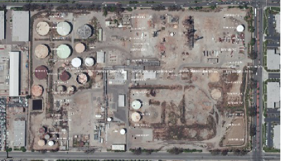
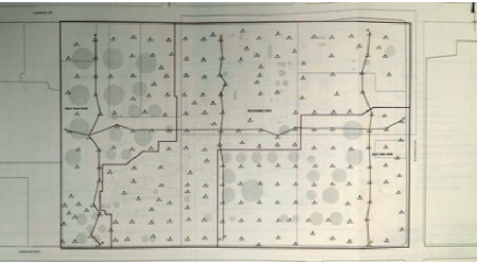
Fig. 1: Aerial photo showing the location of storage tanks (left) and soil boring map (right).

With reference to this specific case study, the sequence of action that we investigate consists of the following steps:

1. Initial spills are assumed to have occurred at the location of the storage tanks shown in Figure 1.

2. Mean and variances of permeability values are associated to soil types throughout the site, resulting in lognormal initial probabilistic models of permeabilities.

3. Physics of flow through porous media yield a corresponding distribution for the concentration of pollutants throughout the site.

4. For a given monitoring design consisting of a set of specific five spatial locations where concentrations are to be observed, a distribution of these observables can be obtained from the previous step.

5. From this distribution of observables, the likelihood for each possible value of observable is calculated, and the Bayesian posterior distribution for that observable is evaluated. Note that at this step, no concentration data is assumed to have been collected yet.

6. The Kullback-Leibler (KL) distance between the prior and the posterior distributions is evaluated as a measure of information gain.

7. The KL distance is integrated over all possible values attained by the observables at the fixed design locations.

8. The optimal monitoring locations are determined by maximizing this averaged KL distance.

9. Measurements of pollutants are taken from the actual field data at the optimal locations.

10. The Bayesian posterior distributions for permeabilities are calculated based on these observations. These posteriors provide an updated description of the permeabilities throughout the site and can be used to improve the prediction of concentration maps over time.

While a stopping criterion for this Bayesian update has been introduced elsewhere [11], it is outside the scope of the present investigation. The paper addresses computational and algorithmic issues required for the implementation of the above steps and provides insight into the computed optimal monitoring strategies.

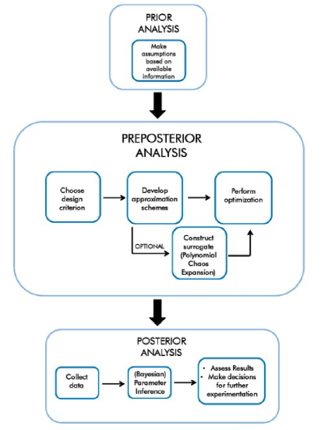
Fig. 2: A flowchart outlining the steps in prior, preposterior and posterior stages of the optimal design methodology.

and is organized as follows. In Section 2 we introduce the design criterion used for experimental design that provides optimal Bayesian inference results and a lower bound that is used as an alternative in the optimization procedure. The stochastic approximation framework required for maximizing the objective function, is described in Section 3. Section 4 provides a toy example in order to justify the use of the lower bound estimate instead of the actual expected information gain as the design criterion. Then our methodology is applied on a real site in Section 5. Precisely, the model is described in subsections 5.1 and 5.2, then a surrogate is constructed in subsection 5.3 in order to accelerate simulations of computationally intensive procedures. The experimental design analysis is performed in subsection 5.4 and the results are validated in subsection 5.5 by estimating the Bayesian update of the uncertain parameters based on data that is generated both for a hypothetical scenario and from field measurements. Our conclusions are summarized in Section 6.

2 Bayesian experimental design

2.1 Design criterion

Our main interest in the present work is to define and evaluate a particular experiment which, constrained by fixed resources, will reduce the prediction uncertainty in some well-defined optimal sense. Let $\mathbf{d}$ denote what we refer to as the set of design parameters. For each choice of these parameters, the experiment design is fixed. Thus $\mathbf{d}$ could, for instance, consist of smoothing kernels that parameterize measurement instruments. Alternatively, as we do in the present work, we construe $\mathbf{d}\in\mathbb{R}^{2m}$ as a vector that defines the spatial coordinates in the horizontal plane of $m$ points at which observations will be obtained. Clearly, $\mathbf{d}$ could also consist of nonlinear functionals. The numerical values of the observations will be denoted by $\mathbf{y}\in\mathbb{R}^{m}$. Prior to conducting the experiments, $\mathbf{y}$ is a random vector. Following the experiment, the numerical values attained by this vector will be used to condition the inference. We make the restrictive assumption that optimal reduction of uncertainty in model-based prediction is attained through an optimal reduction of uncertainty in model parameters which we denote by $\boldsymbol{\theta}$. Relaxing this assumption, while numerically tedious, does not present conceptual difficulties.

2.1.1 Expected information gain

We are thus interested in inferring the unknown parameters $\boldsymbol{\theta}$ that govern the behavior of a physical process. We model these parameters as a vector of random variables. In a Bayesian setting, this inference is carried out by updating the prior distribution $p(\boldsymbol{\theta})$ with a posterior one, namely $p(\boldsymbol{\theta}|\mathbf{y},\mathbf{d})$, given that some specific data $\mathbf{y}$ was observed for particular design parameters $\mathbf{d}$. The posterior distribution is updated according to the rule

(1) $$p(\boldsymbol{\theta}|\mathbf{y},\mathbf{d})=\frac{p(\mathbf{y}|\boldsymbol{\theta},\mathbf{d})p(\boldsymbol{\theta})}{p(\mathbf{y}|\mathbf{d})}$$

where the multi-dimensional integral, $p(\mathbf{y})=\int p(\mathbf{y}|\boldsymbol{\theta},\mathbf{d})p(\boldsymbol{\theta})d\boldsymbol{\theta}$, is referred to as the evidence. Using a Shannon information approach we can define the information gain after updating the distribution of $\boldsymbol{\theta}$ to be the Kullback-Leibler (KL) divergence [20] of the prior and the posterior distributions, that is

(2) $$D_{KL}\left[p(\cdot|\mathbf{y},\mathbf{d})||p(\cdot)\right]=\int_{\Theta}p(\boldsymbol{\theta}|\mathbf{y},\mathbf{d})\log\left[\frac{p(\boldsymbol{\theta}|\mathbf{y},\mathbf{d})}{p(\boldsymbol{\theta})}\right]d\boldsymbol{\theta}.$$

We are interested in quantifying the information gain before the data is actually collected. In the same spirit we define the expected information gain, first proposed by [22] as

(3) $$U(\mathbf{d})=\int_{\mathcal{Y}}D_{KL}\left[p(\cdot|\mathbf{y},\mathbf{d})||p(\cdot)\right]p(\mathbf{y}|\mathbf{d})d\mathbf{y}=\int_{\mathcal{Y}}\int_{\Theta}p(\boldsymbol{\theta}|\mathbf{y},\mathbf{d})\log\left[\frac{p(\boldsymbol{\theta}|\mathbf{y},\mathbf{d})}{p(\boldsymbol{\theta})}\right]d\boldsymbol{\theta}\ p(\mathbf{y}|\mathbf{d})d\mathbf{y}$$

This can be interpreted as follows: The contribution of any possible output that is used as a set of data $\mathbf{y}$ to update to the posterior distribution is given as the KL divergence of the two distributions. Before the data is collected, $U(\mathbf{d})$ provides us with a measure of the average information to be gained. This is a function only of the design parameters $\mathbf{d}$. It is therefore natural to assume that the choice of $\mathbf{d}^{*}$ that offers on average the most informative observations and thus, is the optimal experimental design, is the one that maximizes $U(\mathbf{d})$ and so it satisfies

(4) $$\mathbf{d}^{*}=\arg\max_{\mathbf{d}\in\mathcal{D}}U(\mathbf{d}).$$

Evaluation of the above objective function and therefore its optimization is not a trivial task. At first, one can see that the posterior, being unknown beforehand, needs to be evaluated or approximated. In [23], the posterior was replaced by its Laplace approximation and $U(\mathbf{d})$ was estimated with a sparse quadrature rule. In [31] an alternative form of the objective function was derived by using Bayes’ rule to express the posterior in terms of the evidence, the likelihood and the prior distributions and estimates were proposed via Monte Carlo methods. In both approaches, the maxima were identified by using an exhaustive grid search over the whole design space and limitations due to computational expense were reported. Evaluation of the design criterion on all points of the design space can easily become infeasible in applications where either higher dimensional design parameters are involved or an expensive forward solver is incorporated, hence the need for iterative search strategies is necessary to detect the optimal value. In [15, 16] it was demonstrated that stochastic approximation methods [35] are well adapted to the present situation, when the Monte Carlo estimate of the objective is used and this is the approach we follow in this paper. However, instead of simply adapting the methodology developed in these works, we further derive a lower bound of the expected information gain and its corresponding Monte Carlo estimate to be maximized. The reason for doing so is to overcome computational obstacles that arise from our application: The direct Monte Carlo estimator entails a discretization of the double integral appearing in equation (3) and has been shown to have a bias that is inversely proportional to the number of samples in the inner sum of the estimate, requiring a very large number of inner loop samples for the bias to be negligible [31] (see also Appendix B in [15] for a numerical study). Furthermore, the variance of that estimator is controlled only by the number of the outer loop samples. Expressions for both the bias and variance are given in A. For applications such as the one included in this paper, using tens or hundreds of thousands samples can easily become prohibitive. On the contrary, the lower bound derived below can be easily seen to be unbiased and its variance is controlled by the product of the number of samples used in both loops, something that allows us to achieve the same level of accuracy in our estimate with a much lower number of samples.

2.1.2 Derivation of a lower bound

By substituting $p(\boldsymbol{\theta}|\mathbf{y},\mathbf{d})$ from eq. LABEL:eq:bayes, we write

$$U(\mathbf{d}) = \int_{\mathcal{Y}}\int_{\Theta}\log\left[\frac{p(\boldsymbol{\theta}|\mathbf{y},\mathbf{d})}{p(\boldsymbol{\theta})}\right]p(\boldsymbol{\theta},\mathbf{y}|\mathbf{d})d\boldsymbol{\theta}d\mathbf{y}$$

$$= \int_{\mathcal{Y}}\int_{\Theta}\log\left[p(\mathbf{y}|\boldsymbol{\theta},\mathbf{d})\right]p(\mathbf{y}|\boldsymbol{\theta}|\mathbf{d})p(\boldsymbol{\theta})d\boldsymbol{\theta}d\mathbf{y}-\int_{\mathcal{Y}}\log\left[p(\mathbf{y})\right]p(\mathbf{y}|\mathbf{d})d\mathbf{y}$$

and by denoting with $\mathcal{H}[q(\boldsymbol{\omega})]=-\int\log\left[q(\boldsymbol{\omega})\right]q(\boldsymbol{\omega})d\boldsymbol{\omega}$ the entropy of a distribution $q(\boldsymbol{\omega})$ we take

$$U(\mathbf{d})=-\int_{\Theta}\mathcal{H}[p(\mathbf{y}|\boldsymbol{\theta},\mathbf{d})]p(\boldsymbol{\theta})d\boldsymbol{\theta}+\mathcal{H}[p(\mathbf{y}|\mathbf{d})].$$

In what follows we take the likelihood as a Gaussian distribution with density

$$p(\mathbf{y}|\boldsymbol{\theta},\mathbf{d})=(2\pi)^{-m/2}|\boldsymbol{\Sigma}|^{-1/2}\exp\left\{-\frac{1}{2}\left[\mathbf{y}-\mathcal{G}(\boldsymbol{\theta},\mathbf{d})\right]^{T}\boldsymbol{\Sigma}^{-1}\left[\mathbf{y}-\mathcal{G}(\boldsymbol{\theta},\mathbf{d})\right]\right\}.$$

where the mean is the model output $\mathcal{G}(\boldsymbol{\theta},\mathbf{d})$ and the covariance matrix is $\boldsymbol{\Sigma}$. This is a common choice for models where the observables $\mathbf{y}$ are defined as the model prediction plus some measurement errors

$$\mathbf{y}=\mathcal{G}(\boldsymbol{\theta},\mathbf{d})+\epsilon$$

with the latter being normally distributed with density $\mathcal{N}(0,\boldsymbol{\Sigma})$. In general, the measurement error can be related to the model output through a proportionality factor or even a more complex relation which is typically incorporated in the covariance matrix $\boldsymbol{\Sigma}$. This implies that $\boldsymbol{\Sigma}$ can depend implicitly on both the uncertain and the design parameters. For our purposes we make the rather simple assumption that no such dependence is involved and $\boldsymbol{\Sigma}$ has fixed entries. Further details on the exact values of the covariance matrix including independence among the measurement errors is provided later in our applications.

For the above choice of the likelihood function the entropy can be calculated and is simply

$$\mathcal{H}[p(\mathbf{y}|\boldsymbol{\theta},\mathbf{d})]=\frac{1}{2}\left\{m+\log\left[(2\pi)^{m}|\boldsymbol{\Sigma}|\right]\right\}$$

and we finally get

(5) $$U(\mathbf{d})=-\frac{1}{2}\left\{m+\log\left[(2\pi)^{m}|\boldsymbol{\Sigma}|\right]\right\}+\mathcal{H}[p(\mathbf{y}|\mathbf{d})].$$

At last, using Jensen’s inequality, we derive a lower bound for $U(\mathbf{d})$. Namely we have

$$\mathcal{H}[p(\mathbf{y}|\mathbf{d})]=\int_{\mathcal{Y}}-\log\left[p(\mathbf{y}|\mathbf{d})\right]p(\mathbf{y}|\mathbf{d})d\mathbf{y}\geq-\log\left[\int_{\mathcal{Y}}p^{2}(\mathbf{y}|\mathbf{d})d\mathbf{y}\right]$$

and we define the lower bound of $U(\mathbf{d})$ as

(6) $$U_{L}(\mathbf{d})=-\frac{1}{2}\left\{m+\log\left[(2\pi)^{m}|\boldsymbol{\Sigma}|\right]\right\}-\log\left[\int_{\mathcal{Y}}p^{2}(\mathbf{y}|\mathbf{d})d\mathbf{y}\right]\ .$$

Note that since the common first term of $U(\mathbf{d})$ and $U_{L}(\mathbf{d})$, as they appear in equations (5) and (6), are independent of $\mathbf{d}$, one eventually needs only to maximize the second term, namely the entropy of the marginal distribution of the data or its lower bound. This idea is not new and has been previously used in linear regression models [32] and in geophysical applications [37].

2.1.3 Estimation of the lower bound

As mentioned above, the optimization problem is equivalent to minimizing

$$U^{*}_{L}(\mathbf{d})=\int_{\mathcal{Y}}p^{2}(\mathbf{y}|\mathbf{d})d\mathbf{y}.$$

After expanding the evidence function and writing

$$U^{*}_{L}(\mathbf{d})=\int_{\mathcal{Y}}\int_{\Theta}\int_{\Theta}p(\mathbf{y}|\boldsymbol{\theta}_{1},\mathbf{d})p(\mathbf{y}|\boldsymbol{\theta}_{2},\mathbf{d})p(\boldsymbol{\theta}_{1})p(\boldsymbol{\theta}_{2})d\boldsymbol{\theta}_{1}d\boldsymbol{\theta}_{2}d\mathbf{y}$$

we can see that a Monte Carlo estimate of the above is

(7) $$\hat{U}^{*}_{L}(\mathbf{d})=\frac{1}{NM}\sum_{i,j=1}^{N,M}p(\mathbf{y}^{i}|\boldsymbol{\theta}^{j},\mathbf{d})$$

where $\{\boldsymbol{\theta}^{i}\}$, $\{\boldsymbol{\theta}^{j}\}$, $i=1,...,N$, $j=1,...,M$ are i.i.d. samples from $p(\boldsymbol{\theta})$ and $\{\mathbf{y}^{i}\}$ are i.i.d. samples from $p(\mathbf{y}|\boldsymbol{\theta}^{i},\mathbf{d})$.

3 Stochastic optimization

3.1 Simultaneous perturbation stochastic approximation

Maximization of the objective function derived in the above section can in general be a difficult task. In cases where the design parameters are of high dimension or an expensive forward solver is involved in the evaluation of $U^{*}_{L}(\mathbf{d})$, a direct grid search can easily become prohibitive. Since only a noisy estimate of the actual objective function to be maximized is available, we turn our attention to stochastic approximation methods. These are algorithms that approximate roots of noisy functions and can be used for optimization problems to find the roots of the gradient of the objective function to be optimized. This is done with an iterative procedure of the general form

(8) $$\mathbf{d}_{k+1}=\mathbf{d}_{k}-a_{k}g(\mathbf{d}_{k}),\ \ \ k\geq 0$$

where $\{a_{k}\}_{k\geq 0}$ is a sequence of positive pre-specified deterministic constants, known also as the learning rate of the algorithm and $g(\mathbf{d})=\nabla_{\mathbf{d}}U(\mathbf{d})$ is the gradient of the objective function with respect to $\mathbf{d}$. Algorithms that use an explicit expression for the gradient are called Robbins-Monro algorithms [30] and those where a finite-difference scheme is employed, are called Kiefer-Wolfowitz algorithms [19]. For our purposes we use an algorithm from the Kiefer-Wolfowitz family, namely the Simultaneous Perturbation Stochastic Approximation method (SPSA), proposed by Spall [35, 36]. What makes this methods attractive versus others is the fact that only two forward evaluations are required for the gradient estimation. The updating step of the method is given by

(9) $$\mathbf{d}_{k+1}=\mathbf{d}_{k}-a_{k}\hat{g}_{k}(\mathbf{d}_{k}),$$

where

(10) $$\hat{g}_{k}(\mathbf{d}_{k})=\frac{\hat{U}^{*}_{L}(\mathbf{d}_{k}+c_{k}\boldsymbol{\Delta}_{k})-\hat{U}^{*}_{L}(\mathbf{d}_{k}-c_{k}\boldsymbol{\Delta}_{k})}{2c_{k}}\left[\begin{array}[]{c}\Delta^{-1}_{k,1}\\ \vdots\\ \Delta^{-1}_{k,n_{d}}\end{array}\right],$$

(11) $$a_{k}=\frac{a}{(A+k+1)^{\alpha}},\ \ c_{k}=\frac{c}{(k+1)^{\gamma}}$$

and $a_{k}$, $c_{k}$, $\alpha$, $\gamma$ are positive parameters whose values affect the convergence rate and the gradient estimate. General instructions on how to choose the appropriate values for each problem are given in [36]. The vectors $\boldsymbol{\Delta}_{k}$ are random vectors with coefficients $\Delta_{k,i}$ drawn independently from any zero-mean probability distribution such that the expectation of $|\Delta^{-1}_{k,i}|$ exists [35]. A common choice, which we used in our analysis, corresponds to $\Delta_{k,i}=2(Z-1/2)$ where $Z\sim\mbox{Bernoulli}(p)$ with success probability $p=\frac{1}{2}$.

4 Example: Nonlinear model

4.1 The model and experimental scenarios

The main goal in this example is to explore the accuracy of the lower bound estimate as a substitute for the direct maximization of the expected information gain [15] and provide a numerical comparison of the two approaches. This is achieved by evaluating the two objective functions for a simple algebraic model which is inexpensive to evaluate and is nonlinear with respect to both the uncertain and design parameters. Consider thus the model where the observable quantity $y$ is dependent on $\kappa$ and $d$ as

(12) $$y(\kappa,d) = G(\kappa,d)+\epsilon$$

(13) $$= \kappa^{3}d^{2}+\kappa e^{-|0.2-d|}+\epsilon$$

where $G(\kappa,d)$ is the model output and the noise is taken to be $\epsilon\sim\mathcal{N}(0,10^{-4})$. For prior we choose initially $\kappa\sim\mathcal{U}(0,1)$ and later on we discuss a few more cases. Suppose we have control over $d\in\mathcal{D}$ where $\mathcal{D}=[0,1]$ is the design space and we are interested in inferring $\kappa$. We explore two cases, first the case where inference is carried out using a single observation of $y$ and second the case where two observations of $y$ can be obtained, corresponding to different values of $d$. One can think of the design parameter $d$ as the location where $y$ is observed. Before observing $y$, we would like to know the value of $d$ that would make our observations the most informative ones. Both cases of this example have been studied in [15] using the direct Monte Carlo estimate of $U(d)$. The first case was also studied in [23] using the Laplace approximation of the posterior distribution of $\kappa$ and then performing the integration with sparse quadratures.

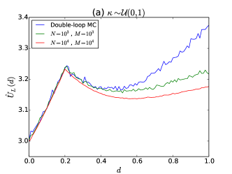
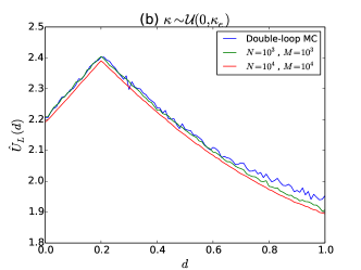
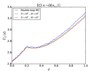
Fig. 3: Expected information gain lower bounds and dlMC with $N=10^{4}$, $M=10^{4}$ estimated over $\mathcal{D}=[0,1]$ for three different priors.

4.2 Results

We are using the expected information gain lower bound estimate as given in (7) as our criterion to determine the optimal design $d$ for inferring $\kappa$. For comparison, we also reproduce the results of [15] using the expected information gain estimate which from now on we call double loop Monte Carlo (dlMC) estimate. The exact expression of the dlMC estimate is given in A. Our computations are performed using an ensemble of samples with $N=M=10^{4}$ for all different priors that we consider below, while keeping the error variance fixed. We demonstrate that the two estimate share the same maxima and their graphs have good quantitative agreement with the lower bound providing slightly less noisy values.

4.2.1 Single observation

Fig. 3 shows the values of estimates of $U_{L}^{*}(d)$ for the design of one experiment after using a $101$-point uniform partition on the design space $\mathcal{D}=[0,1]$ for $N=M=10^{3}$ and for $N=M=10^{4}$ as well as the estimates of dlMC. All cases show the existence of two local maxima at $d=0.2$ and $d=1$. As expected, our estimate always takes values slightly smaller than dlMC, as the former is a lower bound of the latter. Due to the fact that the first term in our estimate (the Gaussian entropy) is a constant, while the first term of the dlMC estimate is a Monte-Carlo approximation of the very same constant, we observe that the lower bound is a smoother curve for the same values of $N$, $M$. Following the slope analysis of [15] we also present the results for two different choices of prior, namely when $\kappa\sim\mathcal{U}(0,\kappa_{e})$ and when $\kappa\sim\mathcal{U}(\kappa_{e},1)$ where $\kappa_{e}=\left[(1-e^{-0.8})/2.88\right]^{1/2}$ which is the point where the slope of $G(\kappa,1)$ becomes greater than the slope of $G(\kappa,0.2)$. For the former case we obtain a global maximum at $d=0.2$ whereas for the latter, the maximum is at $d=1$. At some particular points we can observe that although our estimate is only a lower bound of the dlMC estimate, the value of the dlMC might fall below the value of $U^{*}_{L}(d)$. This, in addition to the fact that we compare noisy estimates of a deterministic quantity, can also emerge as the result of the bias of dlMC which is not negligible for our choice of $M$ (number of inner loop samples). For a more detailed discussion on the bias of dlMC for this example see [15] and for the analytic form of the bias see [31].

4.2.2 Two observations

We calculate the values of $U^{*}_{L}(d_{1},d_{2})$ for $N=M=10^{4}$ over $\mathcal{D}\times\mathcal{D}=[0,1]^{2}$ and we compare them with those of dlMC in Fig. 4. Similar qualitative results as in case 1 can be observed. For $\kappa\sim\mathcal{U}(0,1)$, the points where maximum is attained are $(d_{1},d_{2})=(0.2,1)$ and $(d_{1},d_{2})=(1,0.2)$ which are combinations of the local maxima in the 1-dimensional case. That means that, if two observations can be afforded, they should be taken at the points where local maxima exist for the one observation scenario. The order is insignificant since, as we see, the $U^{*}_{L}(d_{1},d_{2})$ surface is symmetric with respect to the $d_{1}=d_{2}$ line. Similar conclusions are drawn for $\kappa\sim\mathcal{U}(0,\kappa_{e})$ and $\kappa\sim\mathcal{U}(\kappa_{e},1)$ where the maxima are at $(d_{1},d_{2})=(0.2,0.2)$ and $(d_{1},d_{2})=(1,1)$ respectively, as already expected from the results of case 1.

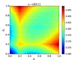
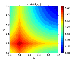
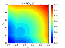
(a) Lower bound estimate $\hat{U}_{L}(\mathbf{d})$

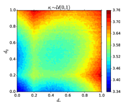
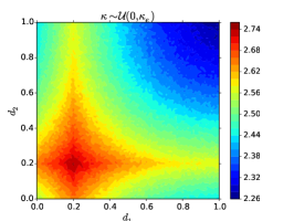
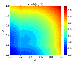
(b) dlMC estimate $\hat{I}(\mathbf{d})$

Fig. 4: Expected information gain lower bound estimate and dlMC estimate with $N=10^{4}$, $M=10^{4}$ for the 2-dimensional design, estimated over $\mathcal{D}=[0,1]^{2}$ for different priors.

5 Example: Case study

This second example demonstrates the application of the formalism to a subsurface pollution characterization problem for an actual site where field data for permeability and concentrations are available.

5.1 Description

We are interested in performing Bayesian inference on the uncertain parameters that affect the transport of pollutants in a contaminated area. Such a procedure will decrease the uncertainty regarding the extent and location of the plume and will further affect the cost and other important aspects of soil remediation. When limited resources are available for experimentation and data collection, it is of great importance to develop experimental design strategies that will enhance the quality of data. Our current study concerns a contaminated site located in Santa Fe Springs, California. Previous data consisting of soil types is available from boreholes located along four cross sections across the site. Each borehole reaches a depth of 20m. Accordingly, soil type is defined as a categorical variable with six possible states. The field and the locations of the boreholes are shown in Figs. 1 and 5 (left). The available soil data is used to construct a domain that can be used in our forward model to simulate the transport of pollutants. The construction of a domain that can be regarded as a good approximation of the real situation, is achieved by the stratigraphic modeling capabilities of the Groundwater Modeling System (GMS) software [1]. More specifically, using a standard inverse-distance weighting based interpolation scheme, we assign soil types for all locations in the area of our interest. The stratigraphy of the resulting domain as well as the extent of each soil are shown in Figs. 5 (right) and 6. Next, the domain was discretized to a $40\times 60\times 10$ grid where each cell has dimensions $15.4$m.$\times 6.7$m.$\times 2$m. and carries the information of the soil type present in that location. The grid is used as our finite volume discretization in the subsequent TOUGH2 simulations and each of the six different soil types present in our domain are assigned different permeability values which, in our study, are considered to be random and are the only source of uncertainty.

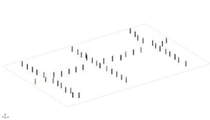
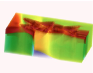
Fig. 5: Boreholes (left) and final domain stratigraphy (right) with the $z$-axis being stretched for the sake of illustration.

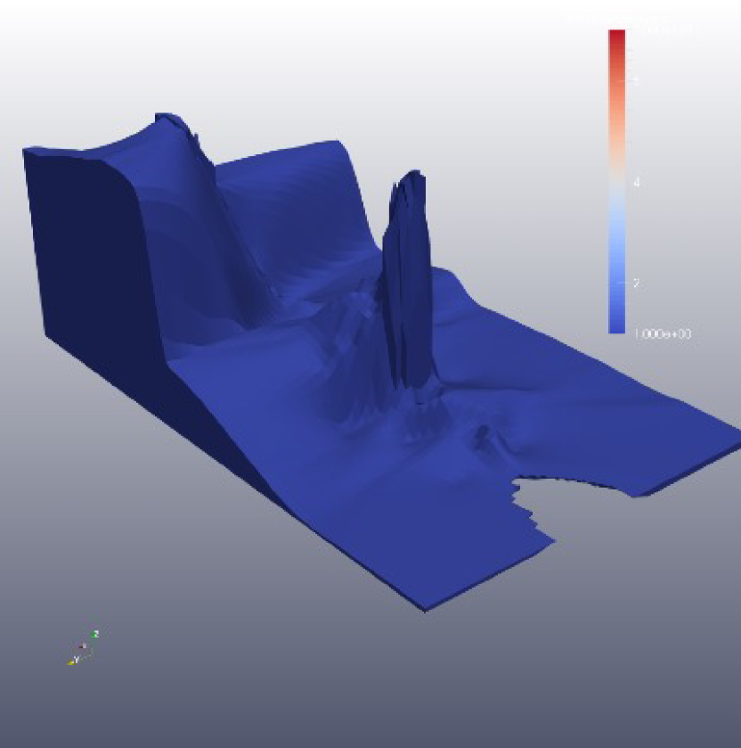
(a) Clay

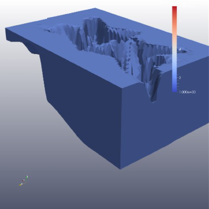
(b) Silt

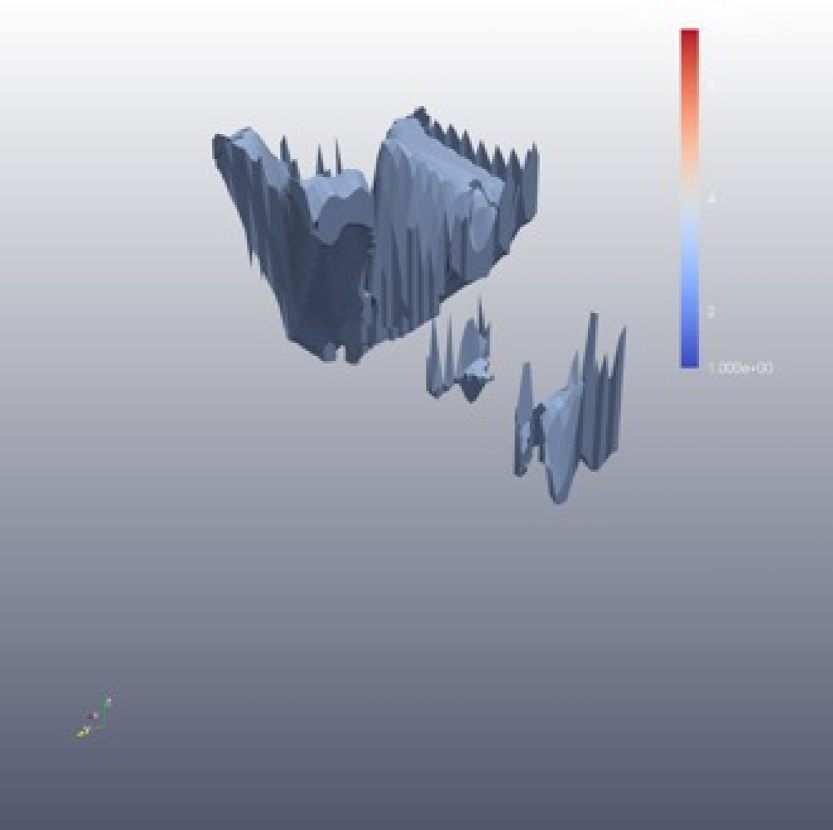
(c) Clayey sand

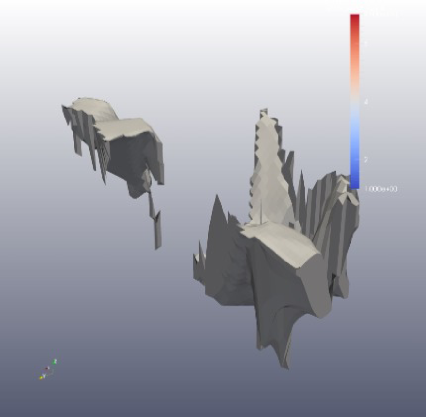
(d) Silty sand

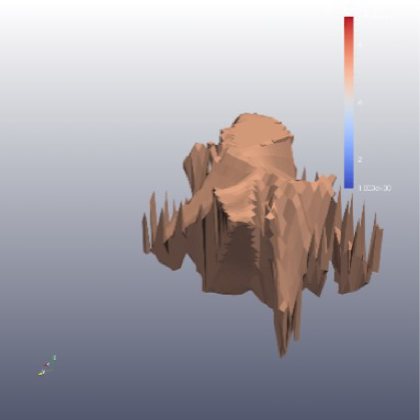
(e) Sand with 10% silt

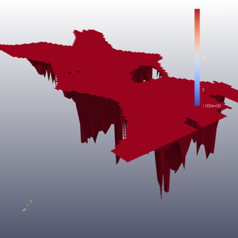
(f) Poorly graded sand

Fig. 6: Soil morphology of the domain. The $z$-axis has been stretched for the sake of illustration.

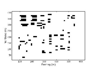
Fig. 7: Locations where initial contaminant injections are placed.

5.2 Simulating flow and transport using TOUGH2

5.2.1 EOS7r module

We employed the multiphase simulator TOUGH2 [28] and its massively parallel version TOUGH2-MP [40] with the EOS7r module to simulate groundwater flow and contaminant transport. TOUGH2 provides us with a finite volume solver which discretizes the mass and energy equations over space and time and updates a set of primary variables that consist the solution of the governing equations by estimating the increments at each time step with a Newton-Raphson method. The common mathematical form of the equations for multiphase fluid flow include several thermophysical parameters such as density, viscosity, enthalpy etc. which are determined by the various ”EOS” (equation-of-state) modules. The EOS7r module [27] used here, is mainly intended to provide radionuclide transport capability but can be as well used for transport of volatile and water soluble organic chemicals (VOCs). Change in concentrations is caused in general for three reasons: transport, decay and adsorption. Volatilization of the VOCs in all phases is modeled by Henry’s law and occurs by advection and diffusion. Decay is modeled by a first-order decay law. In case of radionuclide transport, this is interpreted as radioactive decay but in the case of organic contaminants it can be explained as biodegradation. Adsorption is dependent on the distribution coefficient that characterizes each rocktype. EOS7r in total can simulate transport of five components in a two-phase flow, namely water, air, brine, a parent contaminant and a daughter contaminant in aqueous and gaseous phases.

5.2.2 Santa Fe site

For our problem we are interested in simulating the spreading of organic contaminants in a field located in Santa Fe Springs, CA which is approximately $600m.\times 400m.$ and only $20m.$ deep. This is discretized in TOUGH2 to a grid consisting of $40\times 60\times 10=24000$ active cells where each cell has dimension $15.4m.\times 6.7m.\times 2m.$, as explained in the previous paragraph and is assigned a rocktype according to its soil type. We focus on investigating the propagation of uncertainty emerging from the unknown permeabilities $\boldsymbol{\kappa}=(\kappa_{1},...,\kappa_{6})$ of the six different soil types the are present on our site, through the transport process of the VOCs. The porosity is taken to be uniform $\phi=0.35$ all over the domain. Although we are interested in the transport mainly of petroleum hydrocarbons whose weathering processes are in general known to include adsorption and biodegradation effects, for the purposes of this study we will consider these effects to be of negligible importance by assigning the distribution coefficients for adsorption to be zero and the half-life parameter $\sim 10^{50}$ so that we have no decay effects. Thus our model focuses only on the volatilization properties of the VOCs. We choose the values for the molecular weight and inverse Henry’s constant parameters to correspond to those used for describing transport of petroleum hydrocarbons and specifically those that are mostly detected using gas chromatography techniques, named Gasoline Range Organics (GRO). Typically GRO are the subsets of hydrocarbons in the C5-C12 range and include hydrocarbons such as Benzene, Toluene, Ethylbenzene, m-, o- and p-Xylenes, Naphthalene and Acenaphthene. Their molecular weights are in the $78-154$ grams range. In our case we arbitrarily set the molecular weight to be $112.4$ grams which is a value close to the average GRO hydrocarbon.

Table 1: Material and initial parameters used in our simulations.

Parameter	Symbol	Value
Porosity	$\phi$	$0.35$
Tortuosity factor	$\tau_{0}$	$0.1$
Relative permeability parameters:	$\lambda$	$0.457$
-	$S_{lr}$	$0.15$
-	$S_{ls}$	$1$
-	$S_{gr}$	$0.1$
Capillary pressure parameters:	$\lambda$	$0.457$
-	$S_{lr}$	$0$
-	$1/P_{0}=\alpha/\rho_{w}g$	$5.105e-4$
-	$P_{\max}$	$10^{7}$
-	$S_{ls}$	$1$
Diffusivities (all $k$): gas phase	$d_{g}^{k}$	$10^{-6}$
aqueous phase	$d_{l}^{k}$	$10^{-10}$
Molecular weight	-	$112.4$
Inverse Herny’s constant	-	$2.1\cdot 10^{-8}$
Half-life parameter	-	$10^{50}$
Initial pressure	$P(0)$	$1.013\cdot 10^{5}$
Initial gas saturation	$S_{g}$	$0.75$
Temperature (constant)	$T$	$20^{\circ}$

For our forward evaluations of the model with TOUGH2 we consider that only $3$ components are present by assigning the brine and daughter radionuclide mass fractions to be zero. We assume isothermal conditions with the temperature being constant at $20^{\circ}$C and no-flux boundary conditions. The mathematical formulation of the flow and transport model is described in detail in Appendix B and the values of the model parameters that are assumed known are given in Table 1. Since we want the pressure and gas saturation to be close to steady-state conditions by the time the contaminants are released to the ground, we first run the model for a time period until $T=13.3$ years, where the initial mass fractions for the contaminants is zero. The outputs of pressure and gas saturation are subsequently used as initial conditions for the transport simulation. We rerun the model after assigning initial aqueous phase solubilities for the VOC. We denote these initial conditions with $\mathbf{y}_{0}$. Their locations at time $t=0$ are taken to be approximately in the areas were the storage tanks are located as can be seen in Fig. 7. For our purposes we add $164$ inactive (zero volume) cells to the surface layer of our grid and initial injections are assigned. The exact values were chosen to be $\mathbf{y}_{0}=0.1+U$ ppb (parts per billion) where $U$ are numbers randomly generated from a Uniform distribution with support on $(5\cdot 10^{-5},10^{-2})$ and are considered known. The transport simulation runs for the same time period as the flow simulation.

5.3 Developing a surrogate model

Due to the complexity of our model, only a single simulation of the transport flow with TOUGH2 requires several minutes to finish. Thus, implementing our experimental design framework, including the minimization of the expected information gain lower bound with SPSA which requires thousands of objective function evaluations, becomes impractical. It is therefore necessary to create a surrogate model that would provide us with forward evaluations of the model that are significantly cheaper to obtain than running TOUGH2.

5.3.1 The prior and input transformation

The unknown physical parameters of our problem are the permeabilities $\boldsymbol{\kappa}=(\kappa_{1},...,\kappa_{6})$ of the six materials making-up the subsurface at the site of interest. We choose all $\kappa_{i}$ to be independent with a lognormal prior distribution, that is

(14) $$p(\log\kappa_{i})=\mathcal{N}(-23.5,4)$$

The choice of the mean $\mu=-23.5$ and variance $\sigma^{2}=4$ are made such that our prior covers a range for permeability values in the order of magnitude $10^{-8}$cm² to $10^{-12}$cm² which corresponds to semi-pervious materials. We find this a rather general prior that corresponds solely to our knowledge that the materials present in our domain are silt, clay, silty sand, clayey sand, sand with 10$\%$ silt and poorly graded sand.

Now if we let $F(x)=P(\kappa_{i}\leq x)$ to be the cumulative distribution function of $\kappa_{i}$, then we have that $\xi_{i}:=F(\kappa_{i})\sim U(0,1)$ and for $\boldsymbol{\xi}=(\xi_{1},...,\xi_{6})$ we define $\hat{\mathcal{G}}(\boldsymbol{\xi})=\mathcal{G}(\mathbf{F}^{-1}(\boldsymbol{\xi}),\mathbf{d})$ where $\mathbf{F}(\boldsymbol{\xi})=\prod_{i=1}^{6}F(\xi_{i})$ to be our model output where the input is a set of $6$ independent standard uniform random variables.

5.3.2 Polynomial chaos expansion

We make use of the property that our random output $\hat{\mathcal{G}}(\boldsymbol{\xi})$ is a physical process with finite variance, therefore it is a square-integrable random field $\hat{\mathcal{G}}(\boldsymbol{\xi})\in L^{2}(\mathbb{R}^{m})$, defined on the probability space $([0,1]^{6},\mathcal{F},P)$ and admits a polynomial chaos representation of the form [8, 34, 38]

(15) $$\hat{\mathcal{G}}(\boldsymbol{\xi})=\sum_{\boldsymbol{\alpha},|\boldsymbol{\alpha}|<\infty}\mathbf{p}_{\boldsymbol{\alpha}}\Psi_{\boldsymbol{\alpha}}(\boldsymbol{\xi})$$

where $\boldsymbol{\alpha}=(\alpha_{1},...,\alpha_{d})$ and $\alpha_{i}\in\mathbb{N}^{m}$ for $i=1,...,n$ is a multi-index with modulus $|\boldsymbol{\alpha}|=\alpha_{1}+...+\alpha_{n}$, each $\mathbf{p}_{\boldsymbol{\alpha}}$ is a vector in $\mathbb{R}^{m}$, $\boldsymbol{\xi}$ is a second-order random variable defined on $([0,1]^{6},\mathcal{F},P)$ with values in $\mathbb{R}^{m}$ and the functions $\Psi_{\alpha}$ form a complete set of orthonormal functions that satisfy

(16) $$\mathbb{E}[\Psi_{\boldsymbol{\alpha}}(\boldsymbol{\xi})\Psi_{\boldsymbol{\beta}}(\boldsymbol{\xi})]=\delta_{\boldsymbol{\alpha}\boldsymbol{\beta}}=\delta_{\alpha_{1}\beta_{1}}\times\cdots\times\delta_{\alpha_{d}\beta_{d}}$$

Typically the random variable $\boldsymbol{\xi}$ has independent components that follow a Gaussian, Uniform, Gamma or Beta distribution. The basis function then is chosen to consist of multidimensional polynomials $\Psi_{\boldsymbol{\alpha}}(\boldsymbol{\xi})=\psi_{\alpha_{1}}(\xi_{1})\times\cdots\times\psi_{\alpha_{d}}(\alpha_{n})$, where $\psi_{\alpha_{i}}$ is respectively Hermite, Legendre, Laguerre or Jacobi polynomials of order $\alpha_{i}$. According to the input transformation in the previous paragraph, we take the components of $\boldsymbol{\xi}$ to be $\mathcal{U}(0,1)$ distributed and therefore the polynomials in the expansion will be Legendre. For computational purposes we work with a truncated version of the expression (15) by writing

(17) $$\hat{\mathcal{G}}_{r}(\boldsymbol{\xi})=\sum_{\boldsymbol{\alpha},|\boldsymbol{\alpha}|\leq r}\mathbf{p}_{\boldsymbol{\alpha}}\Psi_{\boldsymbol{\alpha}}(\boldsymbol{\xi}).$$

where the number of terms in the above expansions is

(18) $$N_{\mathbf{p}}=|\{\boldsymbol{\alpha}\in\mathbb{N}^{n},0\leq|\boldsymbol{\alpha}|\leq r\}|=\sum_{j=0}^{r}\frac{(j+n-1)!}{j!(n-1)!}.$$

Eq. (17) provides an accurate approximation of the true model output $\mathbf{y}$ as long as the coefficients $\mathbf{p}_{\boldsymbol{\alpha}}$ are estimated in a fashion that they also incorporate a transformation of $\boldsymbol{\xi}$ to the uncertain parameters of the problem of interest.

5.3.3 Coefficient estimation

In order for the expression (17) to be of use, we need to estimate the coefficients $\mathbf{p}_{\alpha}$. This in general can be done with various methods, mainly categorized as intrusive [39] and nonintrusive methods. We use non-intrusive methods which are easier to implement and more convenient when the forward simulation is seen as a black box. Popular nonintrusive methods include approximating the coefficients by orthogonal projection of the output on the basis functions [9], which involves calculating multidimensional integrals. Other methods calculate the coefficients by solving a linear system of equations constructed after evaluating the model on a set of samples and then either interpolating these points (by choosing collocation points of the polynomial roots [21]) or minimizing the least squares error [41]. The last method is the one adapted here, namely we estimate the coefficients by linear regression taking advantage of the linear dependence of $\hat{\mathcal{G}}_{r}(\boldsymbol{\xi})$ on $\mathbf{p}_{\alpha}$. This requires the evaluation of $\hat{\mathcal{G}}(\boldsymbol{\xi})$ at $N_{\mathcal{G}}$ points $\{\boldsymbol{\xi}^{j}\}_{j=1}^{N_{\mathcal{G}}}$ and then for each component $y_{c}$, $c=1,...,24000$ of the output vector $\hat{\mathcal{G}}=(y_{1},...,y_{24000})^{T}$, we solve the system

(19) $$\mathbf{y}_{c}=\Psi\mathbf{p}_{c},$$

where $\mathbf{y}_{c}=[y_{c}^{1},...,y_{c}^{N_{\mathcal{G}}}]^{T}$, $\Psi$ is the $N_{\mathcal{G}}\times N_{\mathbf{p}}$ matrix formed by evaluating the polynomial basis functions at the $N_{\mathcal{G}}$ selected points and $\mathbf{p}_{c}$ are the vector with the unknown coefficients. The least squares solution of (19) is the one that minimizes $||\Psi\mathbf{p}_{c}-\mathbf{y}_{c}||^{2}$ and is given by

(20) $$\hat{\mathbf{p}}_{c}=(\Psi^{T}\Psi)^{-1}\Psi^{T}\mathbf{y}_{c}$$

provided that $(\Psi^{T}\Psi)^{-1}$ exists. This requires that $N_{\mathcal{G}}\geq N_{\mathbf{p}}$ so that our system will be overdetermined. Again, due to the computationally demanding TOUGH2 forward simulator it is impractical to obtain tens or hundreds of thousand samples so we work with an ensemble of $N_{\mathcal{G}}=1000$ samples which, even on the massively parallel version of TOUGH2 (TOUGH2-MP), with a moderate number of processors used, takes around one week to be generated. This choice of $N_{\mathcal{G}}$ allows us to calculate the coefficients of an expansion of order up to $r=5$. The points $\{\boldsymbol{\xi}^{j}\}_{j=1}^{N_{\mathcal{G}}}$ were randomly selected using Latin Hypercube sampling. In fact, the $5$-order polynomial chaos expansion included $462$ coefficients. This is close to $N_{\mathcal{G}}\approx 2N_{\mathbf{p}}$ which has been suggested as a good choice [14]. New results concerning the stability and $L^{2}$-convergence of Polynomial Chaos approximations obtained via least-squares solutions have been recently reported by [5, 12], however such an analysis falls beyond the scope of this work.

5.3.4 Goodness of fit and truncation error

The next step after obtaining the expansion coefficients is to test how well $\hat{\mathcal{G}}_{r}$ performs as a surrogate. For validation purposes, we estimate the coefficients for $r=1,2,3,4$ and $5$ using all $1000$ samples. We want to test how well the least squares solution fits the samples but also how close $\hat{\mathcal{G}}_{r}$ is to $\hat{\mathcal{G}}$ in the $L^{2}$ sense.

For the first test we employ the common $R^{2}$ statistic known also as coefficient of determination [33] and provides a goodness-of-fit measure for our linear model. The statistic is defined as

(21) $$R^{2}_{c}=1-\frac{RSS_{c}}{\sum_{j=1}^{N_{\mathcal{G}}}(y_{c}^{i}-\bar{y}_{c})^{2}}$$

where the residuals sum of squares is $RSS_{c}=\sum_{j=1}^{N_{\mathcal{G}}}(y_{c}^{j}-y_{c}^{r,j})^{2}$, $c=1,...,24000$.

For the second test, we define the expected relative truncation error as

(22) $$e_{c}=\frac{\mathbb{E}[|\mathcal{G}_{c}(\boldsymbol{\xi})-y_{c}(\boldsymbol{\xi})|^{2}]}{\mathbb{E}[|\mathcal{G}_{c}(\boldsymbol{\xi})|^{2}]}=\frac{\int_{[0,1]^{n}}|\mathcal{G}_{c}(\boldsymbol{\xi})-y_{c}(\boldsymbol{\xi})|^{2}p(\boldsymbol{\xi})d\boldsymbol{\xi}}{\int_{[0,1]^{n}}|\mathcal{G}_{c}(\boldsymbol{\xi})|^{2}p(\boldsymbol{\xi})d\boldsymbol{\xi}},\ \ \ c=1,...,24000$$

where $p(\boldsymbol{\xi})=1$ is the joint distribution of independent $\mathcal{U}(0,1)$’s. The above can be estimated as

(23) $$e_{c}\approx\frac{\sum_{j=1}^{1000}|\mathcal{G}_{c}(\boldsymbol{\xi}^{j})-y_{c}(\boldsymbol{\xi}^{j})|^{2}}{\sum_{j=1}^{1000}|\mathcal{G}_{c}(\boldsymbol{\xi}^{j})|^{2}},\ \ \ c=1,...,24000.$$

Fig. 8 shows the boxplots of the $R^{2}$ statistic, obtained from all components $\mathcal{G}$, of the expansions of order $r=1,...5$ (left) and the boxplots of the relative errors for each order $r=1,...,5$ and for all the components of $\mathcal{G}$ (right). Regarding the $R^{2}$ statistic and particularly for $r=5$ the median is $0.986$ and the lower quartile is above $0.96$ giving us a good fit for the $75\%$ of the expansions along the domain. A thorough look showed that the remaining outputs including outliers for which the fit is not stable correspond to points of the domain that are in the bottom layer and along the east boundary. Regarding the expected truncation error and specifically for the expansions of order $5$ the median is $3.1\cdot 10^{-4}$ and the upper quantile is $10^{-2}$ giving us good approximations in the $L^{2}$ sense. Again the truncation error increases for the points in the bottom layers. To ensure that our experimental design methodology implemented in the next paragraph is unaffected by possible instabilities of the Polynomial Chaos expansions, the model outputs produced for the bottom layer of our domain were not involved in our study.

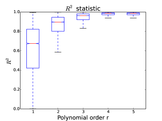
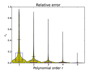
Fig. 8: Boxplots of the $R^{2}$ statistic (left) and relative errors (right) of the polynomial chaoses for all components of the output $\mathcal{G}(\boldsymbol{\xi})$, of order $r=1,...,5$.

5.4 Experimental design

5.4.1 Design settings

As mentioned above, our main goal is to perform Bayesian inference on the permeability parameters that will provide us a tighter posterior that will decrease the uncertainty about the true values of the soil permeability. This will further enhance our current knowledge about the plume location and extent that can potentially result in developing cost-efficient remediation strategies. In order to achieve such a goal, we are seeking the best locations from where data should be collected by employing the expected information gain lower bound as our design criterion.

Unlike the analysis of the nonlinear algebraic model it is clearly understood that in this case, design of a single experiment, that is design for the collection of a single datum would not have important effects in the inference procedure and it is never performed in practice. In our setting we consider that for any location in the $(x,y)$-plane we can observe the concentrations $y$ from the first $5$ layers of our domain, that is up to $10$m. depth, so $5$ data points are available from each location. Without any loss of generality in our method we choose to find the design of experiments consisted of the $5$ best locations in the $(x,y)$-plane from where data will be collected simultaneously to be used for inference. This is a moderate choice which appears to be satisfactory in order to validate our method. Further evaluation of the optimal number of data points is beyond the scope of the present study. The design parameters therefore are $\mathbf{d}=(d_{1,x},d_{1,y},d_{2,x},d_{2,y},...,d_{5,x},d_{5,y})$ where $(d_{i,x},d_{i,y})\in\mathcal{D}_{0}=[0,600]\times[0,400]$, $i=1,...,5$ and the design space for our problem is $\mathcal{D}=\mathcal{D}_{0}^{5}$.

The observations $\mathbf{y}$ are subject to additional measurement noise as indicated from our Gaussian likelihood function $\mathcal{N}(\mathbf{y}|\hat{\mathcal{G}}(\boldsymbol{\xi}),\boldsymbol{\Sigma})$ involved in the expected information gain lower bound derivation. Here we have substituted our forward solver $\mathcal{G}(\boldsymbol{\kappa},\mathbf{d})$ with the polynomial chaos surrogate $\hat{\mathcal{G}}(\boldsymbol{\xi})$. The covariance matrix has been chosen to be $\boldsymbol{\Sigma}=\sigma^{2}\mathbf{I}_{25}$ with $\sigma^{2}=10^{-2}$. This is a rather simple choice that guarantees that measurement errors are independent. A more sophisticated choice would be to take the standard deviation to be proportional to the observable quantity $\sigma=a\hat{\mathcal{G}}_{c}(\boldsymbol{\xi},\mathbf{d})$ where $a$ is some proportionality factor. We avoid this choice as it implies the dependence of the error on the design parameters which contradicts our assumptions for the lower bound derivation.

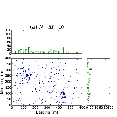
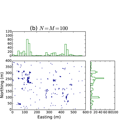
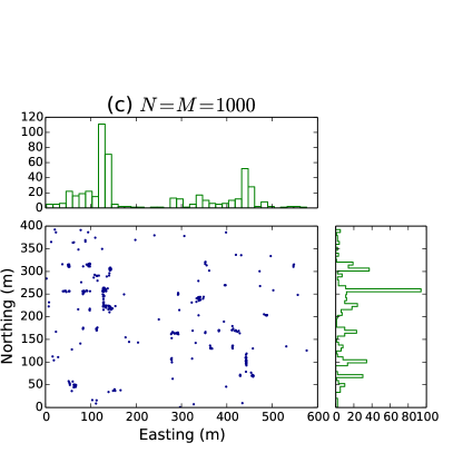
Fig. 9: Scatter plots of the optimal points $d_{i}$ for all optimization solutions $\mathbf{d}^{*}$ of the SPSA algorithm. The red transparent areas denote the locations of the sources, plotted for comparison of the patterns.

5.4.2 Results

We run the SPSA algorithm in order to find $\mathbf{d}$ that minimizes $\hat{U}_{L}^{*}$, therefore maximizes the lower bound estimate. To assess the performance of the algorithm, we run several cases where the choices of $N$ and $M$ in the Monte Carlo loop vary. It is easy to see that the variance of our estimator is

(24) $$var\left[\hat{U}^{*}_{L}(\mathbf{d})\right]=\frac{1}{NM}var\left[p(Y|\boldsymbol{\kappa},\mathbf{d})\right]$$

which shows that $N$ and $M$ have the same contribution in controlling the variance, therefore we take them equal. As stated previously, our estimator is unbiased, unlike the dlMC estimator, so an extremely large value for $M$ is not necessary as it is for dlMC to maintain a low bias. We considered three different cases where $N=M=10,100$ and $1000$. Since the results of SPSA are noisy, in order to better evaluate the performance of the algorithm we obtain the results of $100$ independent runs for each case. For the first two cases we run the algorithm for a total of $10^{4}$ evaluations of the objective function and for the last case we run for $5\cdot 10^{3}$ evaluations. It appears that these choices are rather high since the iterates are stabilized much earlier maintaining a low iteration error.

The resulting $5$-tuples of points in $\mathcal{D}_{0}$ are shown all together in a total of $500$ points in Fig. 9, for all three cases. This gives us a qualitative idea about where the expected information gain is maximized and so data should be collected from. The formation of a certain pattern as $N$, $M$ are increased is obvious and the optimal points appear to be very close to where the contaminant sources were placed. At the same time various points that appear to be outliers are also present, a characteristic behavior of the SPSA algorithm. The case $N=M=10$ particularly shows all points widely spread all over $\mathcal{D}_{0}$ and one can only distinguish the two areas around $(x,y)=(150,250)$ and around $(x,y)=(450,100)$ where more points are accumulated. The cases $N=M=100$ and $N=M=1000$ provide very similar conclusions with the majority of the runs having converged at very specific locations, close to the actual contaminant sources, forming a clear pattern with the main difference that in the third case the points are even more concentrated and less outliers are present.

For a more quantitative argument we also present the exact values of $\hat{U}^{*}_{L}(\mathbf{d})$ as well as those of

(25) $$\hat{U}_{L}(\mathbf{d})=-\frac{1}{2}\left\{m+\log\left[(2\pi)^{m}|\boldsymbol{\Sigma}|\right]\right\}-\log\left[\frac{1}{NM}\sum_{i,j=1}^{N,M}p(\mathbf{y}^{i}|\boldsymbol{\kappa}^{ij},\mathbf{d})\right]$$

calculated at all outcomes $\mathbf{d}^{*}$ of our runs. These values quantify the information gain that each design is expected to offer and at the end, if we had to choose only one design, this should be the design that provides the largest value. This time, for diagnostic reasons and in order to provide a measure of comparison, we want to have a fixed accuracy for the estimates and we use the same number of samples $N=M=1000$ for the evaluation of the two objective functions on all points. Their values are all shown in the histograms presented in Fig. 10. Again there is a significant difference between the quality of the results of the first case with that of the last two cases for both functions. For $\hat{U}^{*}_{L}(\mathbf{d})$, the first case gives us designs that whose values vary in a range from $0.1\cdot 10^{8}$ to $6\cdot 10^{10}$ (observe that the $x$-axis of the histogram is an order of magnitude larger than the rest) with a large number of them being away from the minimum value. The impression one might get for this case is that chances are few that the optimization will yield an optimal design solution and not just an outlier. The other two cases provide similar results with the third being, as expected, better than the second, in the sense that the optimal points are even more concentrated around the minimum value. For completeness we present also $\hat{U}_{L}(\mathbf{d})$ which is technically nothing else but the negative logarithm of $\hat{U}^{*}_{L}(\mathbf{d})$, shifted by a constant. In the first case, the values cover a range from $-3$ to $2.5$ with a mean around $0$. The last two cases give us again similar results with both histograms covering values from around $1$ to $3.5$, a much narrower interval than the first case. Again we can see that the third case is slightly better than the second where we see that the unimodal structure of the histogram is more concentrated on higher values close to $3$ which implies that a few more runs eventually converged to the global maximum.

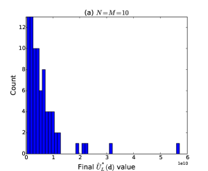
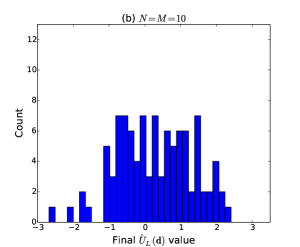
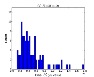
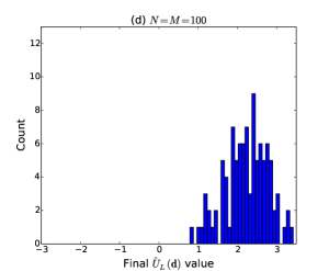
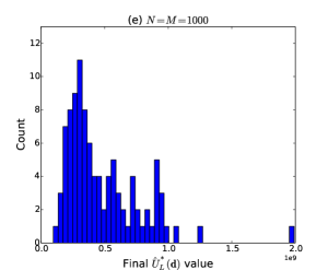
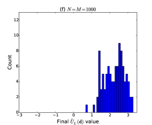
Fig. 10: Histograms of the $\hat{U}^{*}_{L}(\mathbf{d})$ (left) and $\hat{U}_{L}(\mathbf{d})$ (right) values for all optimal points $\mathbf{d}^{*}$.

5.5 Bayesian update of $\log(\kappa)$

In order to validate our methodology and demonstrate the significance of the experimental design analysis developed above, we perform Bayesian inference based on two different designs that are selected according to the results of the previous section. More precisely, data from two different sets of $5$ points, denoted with $\mathbf{d}_{\circ}$ and $\mathbf{d}_{\diamond}$, is collected and used to update the probability distribution of $\boldsymbol{\kappa}$. Specifically, $d_{\circ}$ is selected among the $100$ optimal designs that were approximated by SPSA in the previous section, for $N=M=1000$ and is the one that achieved the maximum $\hat{U}_{L}(\mathbf{d})$ value, so based on the previous analysis it is the design that is expected to yield the best posterior. The second design $\mathbf{d}_{\diamond}$, chosen for comparison only, was arbitrarily selected among the optimal designs that were returned by SPSA using the poor estimate with $N=M=10$ and has a much lower $\hat{U}_{L}(\mathbf{d})$ value, therefore it is expected to update to a wider posterior. The exact location of the points for each set and their $\hat{U}_{L}(\mathbf{d})$ values are shown in Table 2.

Table 2: The $(x,y)$-coordinates of the 5-point designs $\mathbf{d}_{\circ}$ and $\mathbf{d}_{\diamond}$ and their $\hat{U}_{L}(\mathbf{d})$ values.

	$d_{1}$	$d_{2}$	$d_{3}$	$d_{4}$	$d_{5}$	$\hat{U}_{L}(\mathbf{d})$
$\mathbf{d}_{\circ}$	$(127.96,259.65)$	$(442.59,97.05)$	$(143.22,304.41)$	$(337.11,279.02)$	$(412.26,135.86)$	$3.698$
$\mathbf{d}_{\diamond}$	$(22.95,171.37)$	$(75.36,300.00)$	$(318.58,169.27)$	$(425.06,109.96)$	$(441.00,253.70)$	$0.286$

Since the posterior distributions cannot be calculated explicitly, we use Markov Chain Monte Carlo (MCMC) methods to draw samples from them. MCMC methods rely on generating a sequence of random variables based on a Markov Chain that converges to a stationary distribution $\pi(y)$, called the target distribution and therefore the sequence generated after a burn-in period, can be thought of as following the stationary distribution $\pi$. To avoid strong autocorrelation among the samples, appropriate thinning and tuning of the algorithm is required. A powerful MCMC method is the Metropolis-Hastings (MH) algorithm that was first proposed by Metropolis [25] and later generalized by Hastings [13]. The MH algorithm at an arbitrary step generates a new sample $y$ from a proposal distribution $q(x,y)$ given that $x$ is the last accepted sample and accepts it with probability

(26) $$\alpha(x,y)=\min\left\{1,\frac{\pi(y)q(x,y)}{\pi(x)q(y,x)}\right\}.$$

In our case we use the adaptive version of the MH algorithm as developed in [10] with a Gaussian as the proposal distribution where its covariance matrix is updated at each step taking into account all the previous samples that have been drawn. This implies that the chain is non-Markovian, however it has been proved that it has the correct ergodic properties. The adaptive MH (aMH) algorithm provides faster convergence to the target distribution and achieves lower autocorrelation among the samples without very large thinning.

Below we explore two cases where in the first data is observed from a reference field that is associated with one specific realization of the model output while in the second, data is observed from a reference field that is constructed using Gaussian process (GP) regression on measurements taken from the real site.

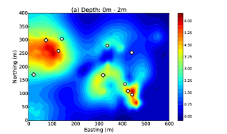
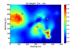
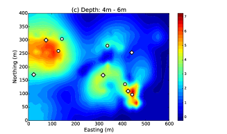
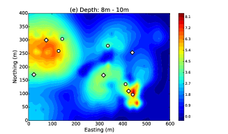
Fig. 11: Concentration map for the $5$ top layers of the domain used as the reference field in example 1. The ’$\circ$’ and ’$\diamond$’ signs indicate the locations of $\mathbf{d}_{\circ}$ and $\mathbf{d}_{\diamond}$ designs respectively, from where measurements were taken.

5.5.1 Case 1: Reference data generated from prior

Here we assume a hypothetical situation where the real permeability values are those displayed on Table 3. Our model’s output for those values can be directly evaluated and the $5$ top layers are displayed in Fig. 11. With this reference field assumed to be our ”reality”, we collect data from the locations indicated at designs $\mathbf{d}_{\circ}$ and $\mathbf{d}_{\diamond}$ and use them for our computations.

Table 3: True values of $\boldsymbol{\kappa}$ and $\log(\boldsymbol{\kappa})$ used for generating the data in case 1.

$i$	$\log\kappa_{i}$	$\kappa_{i}$ (cm2)
$1$	$-22.195$	$2.295\cdot 10^{-10}$
$2$	$-20.791$	$9.346\cdot 10^{-10}$
$3$	$-21.567$	$4.300\cdot 10^{-10}$
$4$	$-25.193$	$1.145\cdot 10^{-11}$
$5$	$-25.272$	$1.058\cdot 10^{-11}$
$6$	$-24.610$	$2.050\cdot 10^{-10}$

We generate $50000$ samples with a $10000$-sample burn-in period and we retain a sample every $5$ steps. After $8000$ samples are obtained, histograms of their values are shown in Fig. 12. Note that the histograms display the marginal distribution of each $\log\kappa_{i}$, $i=1,...,6$ which are no longer independent themselves, however comparison of the histograms for each case together with their priors and the true value gives us an idea about the different results obtained for each design. As expected, we observe that $\mathbf{d}_{\circ}$ provides narrower posteriors that $\mathbf{d}_{\diamond}$. This can be observed particularly on $\log\kappa_{2}$ and $\log\kappa_{5}$ and in a smaller scale on $\log\kappa_{1}$, $\log\kappa_{3}$ and $\log\kappa_{4}$. The posteriors of $\log\kappa_{6}$ for both designs do not display any significant discrepancy from the prior but even in this case the one corresponding to $\mathbf{d}_{\circ}$ appear to be slightly decentralized towards the true value. In addition, for $\mathbf{d}_{\diamond}$ three posteriors, namely $\log\kappa_{2}$, $\log\kappa_{5}$ and $\log\kappa_{6}$ retain their gaussian bell-shaped form and it seems that almost no new information has been gained about their values. This is actually a consequence of the fact that the corresponding soils (silty sand, sand with $10\%$ silt and clay) are not present in the locations where the data was collected from, for this design. Note that clay is present in the lower layers of our domain and not much information is gained about it from $\mathbf{d}_{\circ}$ either. Another general characteristic is that, even for the soils for which both designs provide similar posteriors, the maximum a posteriori values of $\mathbf{d}_{\circ}$ show excellent agreement with the true values while those of $\mathbf{d}_{\diamond}$ show a slight discrepancy which makes them inappropriate for estimation. Overall, we conclude that the design $\mathbf{d}_{\circ}$ provides significantly better inference results that those provided by $\mathbf{d}_{\diamond}$ and this conclusion can be generalized for the comparison of $\mathbf{d}_{\circ}$ with any other design that achieves a lower $\hat{U}_{L}(\mathbf{d})$ value.

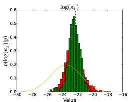
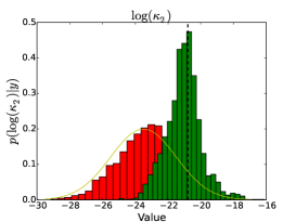
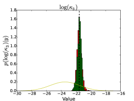
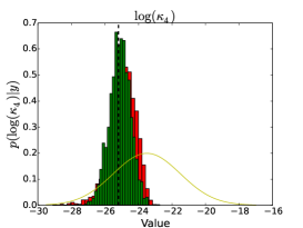
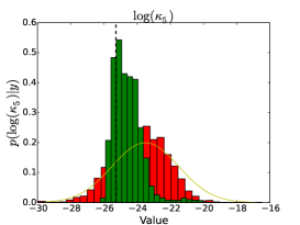
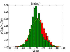
Fig. 12: Comparison of the histograms of the marginal posteriors of all $\log(\kappa_{i})$, $i=1,...,6$ for the designs $\mathbf{d}_{\circ}$ (green) and $\mathbf{d}_{\diamond}$ (red). The red curve indicates their common prior distribution and the dashed black line indicates the true value used to generate the data.

5.5.2 Case 2: Reference data from field measurements

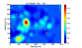
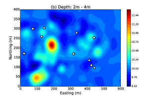
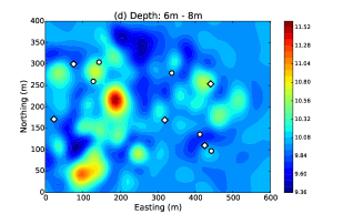
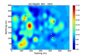
Fig. 13: Concentration map for the $5$ top layers of the domain obtained by GP regression on real data, used as our reference field in example 2. The ’$\circ$’ and ’$\diamond$’ signs indicate the locations of $\mathbf{d}_{\circ}$ and $\mathbf{d}_{\diamond}$ designs respectively, from where measurements were taken.

In this case, the data used in the likelihood function which is incorporated in the acceptance probability through Bayes’ rule, is taken from a reference concentration field, that was generated by GP regression based on measurements taken from the field data at the specified locations as shown in the soil boring map in Fig. 1. These measurements, denoted with $\mathbf{f}$, consist of $1240$ points and their locations form a $1240\times 3$ matrix $X$. Then, if $\mathbf{f}_{*}$ denotes the concentrations over the discretized domain, that is $\mathbf{f}_{*}\in\mathbb{R}^{24000}$, with corresponding locations $X_{*}$, then

(27) $$\mathbf{f}_{*}|X_{*},X,\mathbf{f}\sim\mathcal{N}\left(K(X_{*},X)K(X,X)^{-1}\mathbf{f},K(X_{*},X_{*})-K(X_{*},X)K(X,X)^{-1}K(X,X_{*})\right),$$

where $K(X_{*},X)$ is the covariance matrix with $(K(X_{*},X))_{i,j}=\mathbf{k}(\mathbf{x}_{i},\mathbf{x}_{j})$, $\mathbf{x}_{i}\in X_{*}$, $\mathbf{x}_{j}\in X$ and $\mathbf{k}(\cdot,\cdot)$ denotes some appropriately chosen kernel (for more details on the derivation of this conditional distribution one can see [29]). In our case we chose a squared exponential kernel, given as

(28) $$\mathbf{k}(\mathbf{x},\mathbf{x}^{\prime})=\sigma^{2}\exp\left[-\frac{1}{2}\sum_{n=1}^{3}\frac{(x_{n}-x^{\prime}_{n})^{2}}{\ell^{2}_{n}}\right]$$

which was fit to the data with variance $\sigma^{2}=5$ and correlation lengths $(\ell_{1},\ell_{2},\ell_{3})=(30,30,10)$. Our reference field, consists of the mean $\bar{\mathbf{f}}=K(X_{*},X)K(X,X)^{-1}\mathbf{f}$ and the values of the $5$ top layers are shown in Fig. 13.

Again, we set the posteriors with $p(\boldsymbol{\kappa}|\mathbf{y},\mathbf{d}_{\circ})$ and $p(\boldsymbol{\kappa}|\mathbf{y},\mathbf{d}_{\diamond})$ as our target distributions and this time we generate $100000$ samples with a $10000$-sample burn-in period and we retain a sample every $5$ steps. After $18000$ samples are obtained, histograms of the marginal distributions of each $\log\kappa_{i}$, $i=1,...,6$, are shown in Fig. 14. Again, we observe that $\mathbf{d}_{\circ}$ provides narrower posteriors than $\mathbf{d}_{\diamond}$ for most of the cases. This can be observed particularly on $\log\kappa_{1}$, $\log\kappa_{4}$ and $\log\kappa_{5}$. The posterior of $\log\kappa_{6}$ for the optimal design is almost identical to its prior which implies that nothing new has been learned about its true value. As in the previous example, this is due to the fact that the corresponding soil (clay) is not present in the locations where the data was collected, for this design (recall that clay is present in the lower layers of our domain). In this case, since our data is obtained from a procedure other than evaluating our forward model, it cannot be seen as a direct output of it and generally we do not expect to observe uniqueness of the input parameters that can potentially give rise to our measurements. This is reflected by the fact that different designs give posteriors that seem to concentrate around different values. Bayesian inference however, still provides us with informative results as we observe the posterior distributions to be much further away from the priors, thus learning something about how close our model and our prior assumptions are to the actual reality.

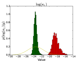
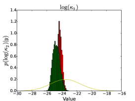
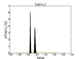
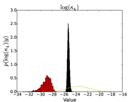
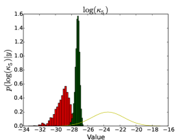
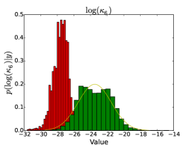
Fig. 14: Comparison of the histograms of the marginal posteriors of all $\log(\kappa_{i})$, $i=1,...,6$ for the designs $\mathbf{d}_{\circ}$ (green) and $\mathbf{d}_{\diamond}$ (red). The red curve indicates their common prior distribution.

6 Conclusions

We presented an experimental design framework that focuses on providing optimal solutions to the design problem in terms of maximizing the information on model parameters from Bayesian inference. This was achieved by employing an information theoretic criterion, namely the expected relative entropy between the prior and the posterior distributions of the unknown parameters. An additional reformulation of the design criterion through the derivation of a lower bound, was of great importance in order to address biasedness issues as well as alleviate the computational burden associated with optimization.

The framework was applied to a real-world problem: The problem of permeability identification in contaminated soils in the presence of experimental field data. The forward model in this case consisted of a system of differential equations that describe contaminant transport in porous media, namely a two-component, two-phase flow-and-transport model that provides as its output the concentrations of the pollutants at the time when data is collected. The design parameters consist of multiple locations where the concentrations will be measured. In the present setting, with the analogous adopted code (TOUGH2) used as a black box simulator, no derivative information was available to the optimization process. The SPSA algorithm, in addition to addressing this issue also seemed to accelerate convergence to the optimal solutions. To further reduce the computational cost, construction of a model surrogate was of crucial importance since the implementation of such a procedure would be impractical otherwise. Finally, our methodology was validated after the inference results showed that the data collected at the optimal design locations were much more informative than the data obtained from other arbitrarily chosen points, in the sense that they resulted in much narrower posteriors, thus gaining more knowledge about the true situation in the subsurface. We observe from our analysis that, under limited resources, the performance of a Bayesian update depends significantly on the location of data acquisition. This highlights the need for optimal monitoring layouts in order to manage environmental risks under economic constraints.

Appendix A Comparison of the expected information gain estimates

A.1 The double-loop Monte-Carlo estimate

The expected information gain can be rearranged in the form

$$I(\mathbf{d})=\int_{\mathcal{Y}}\int_{\mathcal{K}}\left\{\log\left[p(\mathbf{y}|\boldsymbol{\kappa},\mathbf{d})\right]-\log\left[p(\mathbf{y}|\mathbf{d})\right]\right\}p(\mathbf{y}|\boldsymbol{\kappa},\mathbf{d})p(\boldsymbol{\kappa})d\boldsymbol{\kappa}d\mathbf{y}$$

and can be evaluated by using Monte Carlo methods with

$$\hat{I}(\mathbf{d})=\frac{1}{N}\sum_{i=1}^{N}\left\{\log\left[p(\mathbf{y}^{i}|\boldsymbol{\kappa}^{i},\mathbf{d})\right]-\log\left[\frac{1}{M}\sum_{j=1}^{M}p(\mathbf{y}^{i}|\boldsymbol{\kappa}^{i,j},\mathbf{d})\right]\right\},$$

where $\{\boldsymbol{\kappa}^{i}\}$, $\{\boldsymbol{\kappa}^{ij}\}$, $i=1,...,N$, $j=1,...,M$ are i.i.d. samples from $p(\boldsymbol{\kappa})$ and $\{\mathbf{y}^{i}\}$ are i.i.d. samples from $p(\mathbf{y}|\boldsymbol{\kappa}^{i},\mathbf{d})$.

A.2 Properties of the estimates

The properties of $\hat{I}(\mathbf{d})$ are explored in [31]. Precisely it is shown that the variance is proportional to

$$var\left[\hat{I}(\mathbf{d})\right]\propto\frac{A(\mathbf{d})}{N}+\frac{B(\mathbf{d})}{NM}$$

and the bias is proportional to

$$Bias\left[\hat{I}(\mathbf{d})\right]\propto\frac{C(\mathbf{d})}{M},$$

where $A(\mathbf{d})$, $B(\mathbf{d})$ and $C(\mathbf{d})$ are terms that depend on the likelihood and evidence function. Clearly, as mentioned above, $N$ controls the variance and $M$ controls the bias.

For $\hat{U}^{*}_{L}(\mathbf{d})$ we have

$$var\left[\hat{U}^{*}_{L}(\mathbf{d})\right]=\frac{1}{NM}var\left[p(\mathbf{y}|\boldsymbol{\theta},\mathbf{d})\right]$$

and the bias is trivially zero, whereas for $\hat{U}_{L}(\mathbf{d})$ we have

$$var\left[\hat{U}_{L}(\mathbf{d})\right] = var\left[\log\frac{1}{NM}\sum_{i,j=1}^{N,M}p(\mathbf{y}^{i}|\boldsymbol{\theta}^{i,j},\mathbf{d})\right]$$

$$\approx var\left[\log U^{*}_{L}(\mathbf{d})+\frac{\frac{1}{NM}\sum_{i,j=1}^{N,M}p(\mathbf{y}^{i}|\boldsymbol{\theta}^{i,j},\mathbf{d})-U^{*}_{L}(\mathbf{d})}{U^{*}_{L}(\mathbf{d})}\right]$$

$$= var\left[\frac{\frac{1}{NM}\sum_{i,j=1}^{N,M}p(\mathbf{y}^{i}|\boldsymbol{\theta}^{i,j},\mathbf{d})-U^{*}_{L}(\mathbf{d})}{U^{*}_{L}(\mathbf{d})}\right]$$

$$= \frac{1}{NM}\frac{var\left[p(\mathbf{y}|\boldsymbol{\theta},\mathbf{d})\right]}{U^{*}_{L}(\mathbf{d})^{2}},$$

where the second line follows after $1$st-order Taylor expansion about $U^{*}_{L}(\mathbf{d})$ and

$$Bias\left[\hat{U}_{L}(\mathbf{d})\right] = \mathbb{E}\left[\hat{U}_{L}(\mathbf{d})-U_{L}(\mathbf{d})\right]$$

$$= \mathbb{E}\left[-\log\frac{1}{NM}\sum_{i,j=1}^{N,M}p(\mathbf{y}^{i}|\boldsymbol{\theta}^{i,j},\mathbf{d})+\log U^{*}_{L}(\mathbf{d})\right]$$

$$\approx \frac{1}{NM}\frac{var\left[p(\mathbf{y}|\boldsymbol{\theta},\mathbf{d})\right]}{U^{*}_{L}(\mathbf{d})^{2}},$$

where the third line follows after a $2$nd-order Taylor expansion. Here the variance and the bias of the lower bound are controlled by both $N$ and $M$.

Appendix B Governing equations for flow and transport in a porous medium

B.1 Balance equations

The general mass- and energy balance equations in a multicomponent (NK components) multiphase problem are given as

$$\frac{dM^{k}}{dt}=\nabla\cdot\mathbf{F}^{k}+q^{k},\ \ k=1,...,NK,$$

where $k$ is labeling the mass component up to a total of $NK$, $M$ represents mass or energy per volume, $\mathbf{F}$ represents mass or heat flux and $q$ denotes sinks or sources. In some formulations, such as in TOUGH2, an integral expression is used in the form

$$\frac{d}{dt}\int_{V_{n}}M^{k}dV_{n}=\int_{\Gamma_{n}}\mathbf{F}^{k}\cdot\mathbf{n}d\Gamma_{n}+\int_{V_{n}}q^{k}dV_{n},\ \ k=1,...,NK$$

where $V_{n}$ is an arbitrary subdomain of the flow system and $\Gamma_{n}$ its closed boundary surface, $\mathbf{n}$ is a vector normal on the surface element $d\Gamma_{n}$ pointing inward into $V_{n}$. If TOUGH2 is used for the numerical solution of the governing equations, module EOS7r provides consistent characterization of the constitutive equations, allowing a value of NK as high as $5$ (water, air, brine, parent radionuclide, daughter radionuclide). In out problem, a zero source term is assumed resulting in $q=0$ and the contaminant sources in the model are taken to be localized on the surface, at pre-assigned spatial locations shown in Fig. 7. In a TOUGH2 formalism, these sources are modeled as injections in attached zero-volume blocks connected to the gridblocks where the source is assumed to be.

The mass accumulation condition for the $k$th component is

$$M^{k}=\phi\sum_{\beta}S_{\beta}\rho_{\beta}X_{\beta}^{k}$$

where the summation is taken over the fluid phases (liquid, gas, non-aqueous phase liquids). Only liquid and gas phase are considered in our case. The porosity is denoted by $\phi$, $S_{\beta}$ is the saturation of phase $\beta$ (takes values from $0$ to $1$), $\rho_{\beta}$ is the density of phase $\beta$ and $X_{\beta}^{k}$ is the mass fraction of component $k$ present in phase $\beta$.

The advective mass flux is given as

$$\mathbf{F}^{k}_{adv}=\sum_{\beta}X_{\beta}^{k}\mathbf{F}_{\beta}$$

and individual phase fluxed are given by a multiphase version of Darcy’s law:

$$\mathbf{F}_{\beta}=\rho_{\beta}\mathbf{u}_{\beta}=-\kappa\frac{\kappa_{r\beta}\rho_{\beta}}{\mu_{\beta}}(\nabla P_{\beta}-\rho_{\beta}\mathbf{g}).$$

Here $u_{\beta}$ is the Darcy velocity (volume flux) in phase $\beta$, $\kappa$ is the absolute permeability, $\kappa_{r\beta}$ is relative permeability to phase $\beta$, $\mu_{\beta}$ is viscosity and

$$P_{\beta}=P+P_{c\beta}$$

is the fluid pressure in phase $\beta$, which is the sum of the pressure $P$ of a reference phase (usually taken to be the gas phase) and the capillary pressure $P_{c\beta}$ ($\leq 0$), $\mathbf{g}$ is the vector of gravitational acceleration. Vapor pressure lowering due to capillary and phase adsorption effects is modeled by Kelvin’s equation

$$P_{\nu}(T,S_{l})=f_{VPL}(T,S_{l})P_{sat}(T)$$

where

$$f_{VPL}=\exp\left[\frac{M_{w}P_{cl}(S_{l})}{\rho_{l}R(T+273.15)}\right]$$

is the vapor pressure lowering factor. Phase adsorption is neglected. The saturated vapor pressure of bulk aqueous phase is denoted by $P_{sat}$, $P_{cl}$ is the difference between aqueous and gas phase pressures, $M_{w}$ is the molecular weight of water and $R$ is the universal gas constant. Temperature $T$ is assumed constant.

The absolute permeability of the gas phase increases at low pressures according to the relation given by Klinkenberg

$$\kappa=\kappa_{\infty}\left(1+\frac{b}{P}\right)$$

where $\kappa_{\infty}$ is the permeability at ”infinite” pressure and $b$ is the Klinkenberg parameter. In addition to Darcy’s flow, mass flux occurs by molecular diffusion according to

$$\mathbf{f}^{k}_{\beta}=-\phi\tau_{0}\tau_{\beta}\rho_{\beta}d_{\beta}^{k}\nabla X_{\beta}^{k}.$$

Here $d_{\beta}^{k}$ is the molecular diffusion coefficient for component $k$ in phase $\beta$, $\tau_{0}\tau_{\beta}$ is the tortuosity which includes a porous medium dependent factor $\tau_{0}$ and a coefficient that depends on phase saturation $S_{\beta}$, $\tau_{\beta}=\tau_{\beta}(S_{\beta})$. Finally, the total mass flux is finally given by

$$\mathbf{F}^{k}=\mathbf{F}_{abd}+\sum_{\beta}\mathbf{f}_{\beta}^{k}.$$

B.2 Relative permeability model

The relative permeability is assumed to follow the van Genuchten-Mualem model which for liquid is

$$\kappa_{rl}=\left\{\begin{array}[]{lc}\sqrt{S^{*}}\left[1-\left(1-S^{*1/\lambda}\right)^{\lambda}\right]^{2},&S_{l}<S_{ls}\\ 1,&S_{l}\geq S_{ls}\end{array}\right.$$

and for gas is

$$\kappa_{rg}=\left\{\begin{array}[]{lc}1-\kappa_{rl},&if\ S_{gr}=0\\ \left(1-\hat{S}\right)^{2}\left(1-\hat{S}^{2}\right),&if\ S_{gr}>0\end{array}\right.$$

subject to restriction $0\leq\kappa_{rl},\kappa_{rg}\leq 1$. Here $S^{*}=(S_{l}-S_{lr})/(S_{ls}-S_{lr})$ and $\hat{S}=(S_{l}-S_{lr})(1-S_{lr}-S_{gr})$.

B.3 Capillary pressure model

For the capillary pressure we use the van Genuchten function given as

$$P_{cap}=-P_{0}\left(S^{*-1/\lambda}-1\right)^{1-\lambda}$$

subject to restrictions $-P_{\max}\leq P_{cap}\leq 0$. Again $S^{*}$ is defined as for the relative permeability.

B.4 Parameters

Table 1 displays the nominal values assigned to all parameters required according to the above governing equations. It is important also to note the following for our simulation:
1. The mobilities are upstream weighted.
2. The permeabilities are harmonic weighted.
3. Module EOS7r currently neglects brine and daughter radionuclide, resulting in a 3-component flow.
4. Adsorption effects are neglected.
5. Biodegradation effects are neglected.

References

- [1] Aquaveo, L.L.C., 2007. Groundwater Modeling System Version 6.5.6, build date, May 27, 2009, UT, USA.
- [2] A.C. Atkinson and A.N. Donev. Optimum experimental design with SAS. Oxford Statistical Science Series, Oxford University Press, 2007.
- [3] D.A. Baú and A.S. Mayer. Optimal design for pump-and-treat under uncertain hydraulic conductivity and plume distribution. Journal of Contaminant Hydrology, 100:30–46, 2008.
- [4] K. Chaloner and I. Verdinelli. Bayesian experimental design: a review. Statistical Science, 10:273–304, 1995.
- [5] A. Cohen, M.A. Davenport, and D. Leviatan. On the stability and accuracy of leats squares approximations. Foundations of Computational Mathematics, 13:819–834, 2013.
- [6] V.V. Fedorov. Theory of optimal experiments. Academic Press, New York, 1972.
- [7] R.A. Freeze, B. James, J. Massmann, T. Sperling, and L. Smith. Hydrogeological decision analysis, 4: The concept of data worth and its use in the development of site investigation strategies. Ground Water, 30:574–588, 1992.
- [8] R.G. Ghanem and P.D. Spanos. Stochastic finite elements: A spectral approach, revised edition. Dover Publications Inc, 2012.
- [9] D.M. Ghiocel and R.G. Ghanem. Stochastic finite element analysis of seismic soil structure interaction. Journal of Engineering Mechanics, 128:66–77, 2002.
- [10] H. Haario, E. Saksman, and J. Tamminen. An adaptive metropolis algorithm. Bernoulli, 7:223–242, 2001.
- [11] H. Haddad-Zadegan, R. Ghanem, and P. Hajali. Data worth analysis in spatial prediction and soil remediation. In G. Deodatis and B. Ellingwood, editors, ICOSSAR’13: International Conference on Structural Safety and Reliability, Columbia University, June 16-20 2013.
- [12] J. Hampton and A. Doostan. Coherence motivated sampling and convergence analysis of least-squares polynomial chaos regression. arXiv preprint, arXiv:1410.1931, 2014.
- [13] W.K. Hastings. Monte carlo sampling methods using markov chains and their applications. Biometrika, 57:97–109, 1970.
- [14] S. Hosder, R.W. Walters, and M Balch. Efficient sampling for non-intrusive polynomial chaos applications with multiple uncertain input variables. In 9th AIAA Non-Deterministic Approaches Conference, 2007.
- [15] X. Huan and Y. Marzouk. Simulation-based optimal bayesian experimental design for nonlinear systems. Journal of Computational Physics, pages 288–317, 2013.
- [16] X. Huan and Y. Marzouk. Gradient-based stochastic optimization methods in bayesian experimental design. International Journal for Uncertainty Quantification, 4:479–510, 2014.
- [17] B.R. James and R.A. Freeze. The worth of data in predicting aquitard continuity in hydrogeological design. Water Resources Research, 29:2049–2065, 1993.
- [18] B.R. James and S.M. Gorelick. When enough is enough: The worth of monitoring data in aquifer remediation design. Water Resources Research, 30:3499–3513, 1994.
- [19] J. Kiefer and J. Wolfowitz. Stochastic estimation of a regression function. The Annals of Mathematical Statistics, 23:462–466, 1952.
- [20] S. Kullback and R.A. Leibler. On information and sufficiency. The Annals of Mathematical Statistics, 22:79–86, 1951.
- [21] H. Li and D. Zhang. Probabilistic collocation method for flow in porous media: Comparisons with other stochastic methods. Water Resources Research, 43:44–56, 2007.
- [22] D. V. Lindley. On a measure of the information provided by an experiment. The Annals of Mathematical Statistics, 27:986–1005, 1956.
- [23] Q. Long, M. Scavino, R. Tempone, and S. Wang. Fast estimation of expected information gains for bayesian experimental designs based on laplace approximations. Computational Methods in Applied Mechanics and Engineering, 259, 2013.
- [24] J. Massmann and R.A. Freeze. Groundwater contamination from waste management sites: The interaction between risk-based engineering design and regulatory policy:1. methodology. Water Resources Research, 23:351–367, 1987.
- [25] N. Metropolis, A.W. Rosenbluth, M.N. Rosenbluth, A.H. Teller, and E. Teller. Equations of state calculations by fast computing machines. Journal of Chemical Physics, 21:1087–1091, 1953.
- [26] T. Norberg and L. Rosén. Calculating the optimal number of contaminant samples by means of data worth analysis. Environmetrics, 17:705–719, 2006.
- [27] C. Oldenburg and K. Pruess. EOS7R: Radionuclide transport for TOUGH2. Berkeley, California, November 1995. Report LBL-34868.
- [28] K. Pruess, C. Oldenburg, and G. Moridis. TOUGH2 User’s guide, Version 2. Berkeley, California, 1999. Report LBNL-43134.
- [29] C.E. Rasmussen and C.K.I. Williams. Gaussian processes for machine learning. The MIT Press, 2006.
- [30] H. Robbins and S. Monro. A stochastic approximation method. The Annals of Mathematical Statistics, 22:400–407, 1951.
- [31] K.J. Ryan. Estimating expected information gains for experimental designs with application to the random fatigue-limit model. Journal of Computational and Graphical Statistics, 12:585–603, 2003.
- [32] P. Sebastiani and H.P. Wynn. Maximum entropy sampling and optimal bayesian experimental design. Journal of the Royal Statistical Society. Series B: Statistical Methodology, 62:145–157, 2000.
- [33] G.A.F. Seber and A.J. Lee. Linear regression analysis, second edition. John Wiley and Sons, 2003.
- [34] C. Soize and R. Ghanem. Physical systems with random uncertainties: Chaos representations with arbitrary probability measure. SIAM Journal of Scientific Computing, 26(2):395–410, 2004.
- [35] J.C. Spall. Multivariate stochastic approximation using a simultaneous perturbation gradient approximation. IEEE Transactions on Automatic Control, 37, 1992.
- [36] J.C. Spall. Implementation of the simultaneous perturbation algorithm for stochastic optimization. IEEE Transactions on Aerospace and Electronic Systems, 34, 1998.
- [37] J. van den Berg, A. Curtis, and J. Trampert. Optimal nonlinear bayesian experimental design: an application to amplitude versus offset experiments. Geophysical Journal International, 155:411–421, 2003.
- [38] D. Xiu and G.E. Karniadakis. The wiener-askey polynomial chaos for stochastic differential equations. SIAM Journal of Scientific Computing, 24:619–644, 2002.
- [39] D. Xiu and G.E. Karniadakis. Modeling uncertainty in flow simulations via generalized polynomial chaos. Journal of Computational Physics, 187:137–167, 2003.
- [40] K. Zhang, Y.S. Wu, and K. Pruess. User’s guide for TOUGH2-MP - A massively parallel version of the TOUGH2 code. Berkeley, California, 2008. Report LBNL-315E.
- [41] Y. Zhang and N.V. Sahinidis. Uncertainty quantification in co2 sequestration using surrogate models from polynomial chaos expansion. Industrial & Engineering Chemistry Research, 52:3121–3132, 2012.