A coupled-channel formalism for three-body final state interaction

Abstract

From dispersion relation approach, a formalism that describes final state interaction among three particles in a coupled-channel system is presented. Different representations of coupled-channel three-body formalism for spinless particles in both initial and final states are derived.

Introduction.—Hadron spectroscopy is one of important methods for studying non-perturbative QCD and gaining insights of hadron structures and decay mechanism. With high statistic data collected from facilities, such as BESIII, Jefferson Lab and Panda, data analysis becomes even more challenging than ever before, especially, multiparticle dynamics may play the central pole in inelastic region, without proper consideration of constraints from physics principles and multiparticle dynamics, amplitudes extracted from data may be misleading. Therefore, to understand phenomena precisely, theoretical description of decay amplitudes need to take into account all possible dynamics, and follow some basic physics principles, such as unitarity and analyticity. In the past, handling processes with multiple-particle final states has been mainly based on the isobar model Goradia:1975ec ; Ascoli:1975mn , i.e. assuming a multiparticle decay proceeded through a series of quasi-two-body sequential decays. For example, a decay process of one particle (0) into three final states (1,2,3) is usually described by a sum of all possible decay chains: $0\rightarrow(12)3+1(23)+(31)2\rightarrow 123$. For each individual decay chain, the amplitude is a product of kinematic factors, a coupling constant and a two-body amplitude that only depends on two-particle subenergy. Interaction among multiple final state particles has been ignored completely in the isobar model.

Three-body correction to isobar model has been developed since 1960 Khuri:1960zz ; Bronzan:1963kt ; Aitchison:1965kt ; Aitchison:1965dt ; Aitchison:1966kt ; Pasquier:1968zz ; Pasquier:1969dt ; Dodd:1977pj ; Kambor:1995yc ; Schneider:2011dt ; Schneider:2012ez ; Guo:2014vya ; Guo:2014mpp ; Danilkin:2014cra ; Guo:2015zqa , which is based on subenergy dispersion relation approach by considering the unitarity and analyticity properties of amplitudes. In those dispersive approaches Aitchison:1965kt ; Aitchison:1965dt ; Aitchison:1966kt ; Pasquier:1968zz ; Pasquier:1969dt ; Kambor:1995yc ; Schneider:2011dt ; Schneider:2012ez ; Guo:2014vya ; Guo:2014mpp ; Danilkin:2014cra ; Guo:2015zqa , a decay amplitude is written as the sum of all possible decay chains. For each individual decay chain, the amplitude now is the product of kinematic factors, a subenergy dependent complex scalar function. This scalar function satisfies a coupled dispersion relation equations, and the solutions of these equations describe the rescattering effects among three particles. In this approach, interaction among three particles is generated from pair-wise two-body interactions by exchanging a particle between pairs. The unitarity and analyticity are guaranteed naturally. However, all the previous developments have not considered the contribution from inelastic channels yet. In reality, the subenergy in the most of hadron production processes usually is far beyond the elastic region. Once inelastic channels open up, the interference between different channels may be important Guo:2010gx ; Guo:2011aa . In recent years, the demand for studying and including three-body effect has been increased significantly, such as, for excited baryon study at Jefferson Lab. The complication for establishing higher excited baryon states in those studies are not only because most of those baryon states are produced from multiple-particle final states but also from the strongly coupled multiple channels in inelastic region. Similar situation may exist in incoming exotic mesons studies at Hall D, Jefferson Lab and ongoing excited charmonium studies at BES III. Therefore, to disentangle all the coupled-channel effects from the multiple-particle final state interaction, a coupled-channel formalism for multiple-particle states is essential, some efforts based on effective theory formalism have been made along this line Kamano:2011ih ; Nakamura:2012xx ; Nakamura:2015qga . The goal of this work is to generalize dispersive three-body rescattering formalism to include the channels in inelastic region. In this letter, the decay process of a spinless-particle to three spinless-particle is presented to demonstrate the basics of coupled-channel three-body formalism without complication of spin structure of particles.

Basic representation of coupled-channel three-body formalism.—The decay of a spinless particle to three spinless particles is described by,

$$\langle 1(\alpha)2(\beta)3(\gamma),\mbox{out}|0,\mbox{in}\rangle=i(2\pi)^{4}\delta^{4}(\sum_{i=1,2,3}p_{i}-P)T^{\alpha\beta\gamma},$$ (1)

where $(\alpha,\beta,\gamma)$ stand for the species of final state particles $(1,2,3)$ respectively, and the four momenta of i-th final state particle and the parent particle are denoted by $p_{i}$ and $P$ respectively. The decay amplitude $T^{\alpha\beta\gamma}$ are usually expressed as the sum of partial wave series in each two-body subenergy-channel Khuri:1960zz ; Bronzan:1963kt ; Aitchison:1965kt ; Aitchison:1965dt ; Aitchison:1966kt ; Pasquier:1968zz ; Pasquier:1969dt ,

$$T^{\alpha\beta\gamma}=\sum_{L}(2L+1)\left[P_{L}(z_{\alpha\beta})F^{(\alpha\beta)}_{L}(s_{12})\right.$$

$$\quad\quad\quad\left.+P_{L}(z_{\beta\gamma})F^{(\beta\gamma)}_{L}(s_{23})+P_{L}(z_{\gamma\alpha})F^{(\gamma\alpha)}_{L}(s_{31})\right],$$ (2)

where the isospin couplings have been suppressed for simplification purpose only, the invariants are defined by $s_{ij}=(p_{i}+p_{j})^{2}$ and three invariants are constrained by relation: $s_{12}+s_{23}+s_{31}=M^{2}+m_{\alpha}^{2}+m_{\beta}^{2}+m_{\gamma}^{2}$ ($M$ and $m$’s label parent and final state particle masses respectively). The total spin of two-particle subsystem is labeled by $L$. The cosine of polar angle of particle-1 in the rest frame of ($1(\alpha)2(\beta)$) system, $z_{\alpha\beta}=\cos\theta_{\alpha\beta}$, is given by ,

$$z_{\alpha\beta}=-\frac{s_{12}(s_{23}-s_{31})+(m_{\alpha}^{2}-m_{\beta}^{2})(M^{2}-m^{2}_{\gamma})}{2Mp_{\gamma}(s_{12})2\sqrt{s_{12}}q_{\alpha\beta}(s_{12})},$$ (3)

where the momentum factors $q$ and $p$ are defined by

$$q_{\alpha\beta}(s_{12})=\frac{\sqrt{\left[s_{12}-(m_{\alpha}-m_{\beta})^{2}\right]\left[s_{12}-(m_{\alpha}+m_{\beta})^{2}\right]}}{2\sqrt{s_{12}}},$$

$$p_{\gamma}(s_{12})=\frac{\sqrt{\left[s_{12}-(M-m_{\gamma})^{2}\right]\left[s_{12}-(M+m_{\gamma})^{2}\right]}}{2M}.$$ (4)

Similarly, the other $z$’s are given by cyclically permutating sub- and super-indices of Eqs.(3) and (4). The dynamics of decay process are described by scalar functions $F$’s, which only depend on subenergy of isobar pair ($s_{ij}$) by assumption.

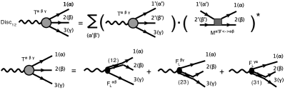
Figure 1: A diagrammatic representation of discontinuity relations in Eq.(A coupled-channel formalism for three-body final state interaction), the partial wave projection of Eq.(A coupled-channel formalism for three-body final state interaction) gives Eq.(7) .

Considering the analytic properties of decay amplitude $T^{\alpha\beta\gamma}$, the discontinuity crossing unitarity cut in subenergy, e.g. $s_{12}$, then reads,

$$\mbox{Disc}_{12}T^{\alpha\beta\gamma} (p_{1},p_{2},p_{3})$$

$$= \frac{1}{2}\sum_{(\alpha^{\prime}\beta^{\prime})}\int\frac{d^{3}\mathbf{p}^{\prime}_{1}}{(2\pi)^{3}2p^{{}^{\prime}0}_{1}}\frac{d^{3}\mathbf{p}^{\prime}_{2}}{(2\pi)^{3}2p^{{}^{\prime}0}_{2}}$$

$$\times(2\pi)^{4}\delta^{4}(p_{1}+p_{2}-p^{\prime}_{1}-p^{\prime}_{2})$$

$$\times\mathcal{M}_{\alpha\beta\leftrightarrow\alpha^{\prime}\beta^{\prime}}^{*}(p_{1}p_{2};p^{\prime}_{1}p^{\prime}_{2})T^{\alpha^{\prime}\beta^{\prime}\gamma}(p^{\prime}_{1},p^{\prime}_{2},p_{3})$$

$$+ \sum_{L}(2L+1)P_{L}(z_{\alpha\beta})\sigma^{(\alpha\beta)}_{L}(s_{12}),$$ (5)

where the summation of $(\alpha^{\prime}\beta^{\prime})$ run over all allowed two-body intermediate states for $(1^{\prime}(\alpha^{\prime})2^{\prime}(\beta^{\prime}))$ pair, last term $\sigma^{(\alpha\beta)}_{L}$ denotes the contribution from the rest of inelastic channels. In current work, our discussion will be only limited to the three-body subspace of inelastic channels by choosing $\sigma^{(\alpha\beta)}_{L}=0$. The partial wave expansion of two-body scattering amplitude $\mathcal{M}$ in a coupled-channel system is given by

$$\mathcal{M}_{\alpha\beta\leftrightarrow\alpha^{\prime}\beta^{\prime}}(p_{1}p_{2};p^{\prime}_{1}p^{\prime}_{2})$$

$$=(16\pi)\sum_{L}(2L+1)P_{L}(\cos\theta)\left[t_{L}(s_{12})\right]_{(\alpha\beta),(\alpha^{\prime}\beta^{\prime})},$$ (6)

where $\theta$ is the angle between incoming and outgoing particles of two-particle system. The matrix $t_{L}$ denotes coupled-channel partial wave scattering amplitudes and it is normalized to $\mbox{Im}t_{L}^{-1}=-\rho$, where the non-vanishing elements of diagonal matrix $\rho$ are given by $\rho_{\alpha\beta}=2q_{\alpha\beta}/\sqrt{s_{12}}$. A diagrammatic representation of discontinuity relations in Eq.(A coupled-channel formalism for three-body final state interaction) is shown in Fig. 1. Commonly, the kinematical singularities are pulled out from decay amplitudes by defining $\widehat{F}^{(\alpha\beta)}_{L}(s_{12})=F^{(\alpha\beta)}_{L}(s_{12})/\left[\sqrt{s_{12}}q_{\alpha\beta}(s_{12})p_{\gamma}(s_{12})\right]^{L}$ Guo:2010gx ; Guo:2011aa , where $\widehat{F}^{(\alpha\beta)}_{L}$ possess only dynamical unitarity cuts by assumption. The discontinuity relations for scalar functions $\widehat{F}^{(\alpha\beta)}_{L}(s_{12})$ are then derived from Eqs.(A coupled-channel formalism for three-body final state interaction) and (A coupled-channel formalism for three-body final state interaction),

$$\mbox{Disc}_{12} \widehat{F}^{(\alpha\beta)}_{L}(s_{12})$$

$$= \sum_{(\alpha^{\prime}\beta^{\prime})}\frac{\left[t^{*}_{L}(s_{12})\theta(s_{12}-s_{R})\rho(s_{12})\right]_{(\alpha\beta),(\alpha^{\prime}\beta^{\prime})}}{\left[\sqrt{s_{12}}q_{\alpha\beta}(s_{12})p_{\gamma}(s_{12})\right]^{L}}$$

$$\times\frac{1}{2}\int_{-1}^{1}dz_{\alpha^{\prime}\beta^{\prime}}P_{L}(z_{\alpha^{\prime}\beta^{\prime}})T^{\alpha^{\prime}\beta^{\prime}\gamma}(s_{12},s_{23},s_{31}),$$ (7)

where the non-vanishing elements of diagonal matrix $s_{R}$ are $s^{(\alpha\beta)}_{R}=(m_{\alpha}+m_{\beta})^{2}$. The self-consistent integral equation for $\widehat{F}^{(\alpha\beta)}_{L}(s_{12})$ is constructed by dispersion relation,

$$\widehat{F}^{(\alpha\beta)}_{L}(s_{12})=\frac{1}{\pi}\int_{s^{(\alpha\beta)}_{R}}^{\infty}ds^{\prime}\frac{\mbox{Disc}_{12}\widehat{F}^{(\alpha\beta)}_{L}(s^{\prime})}{s^{\prime}-s_{12}},$$ (8)

where we have assumed that $\mbox{Disc}_{12}\widehat{F}^{(\alpha\beta)}_{L}(\infty)=0$, so that no subtractions is needed. The angular projection in Eq.(7) has to be analytically continued when discontinuity relation of $\widehat{F}_{L}$’s is plugged into Eq.(8), especially in the situation when the dispersion integral runs out of physical decay region, $z$’s are no longer defined on real axis between $-1$ and $1$. The procedure of analytic continuation has been given in Khuri:1960zz ; Bronzan:1963kt ; Aitchison:1965kt ; Aitchison:1965dt ; Aitchison:1966kt ; Pasquier:1968zz ; Pasquier:1969dt . Similarly, sets of equations for $\widehat{F}^{(\beta\gamma)}_{L}(s_{23})$ and $\widehat{F}^{(\gamma\alpha)}_{L}(s_{31})$ can be constructed in exactly the same approach, and together with Eq.(8), they form a set of close coupled equations. The solutions of coupled-equation for $F$’s describe the three-body rescattering contribution from both elastic and inelastic three-body channels. Eqs.(7) and (8) yield a basic representation of coupled-channel formalism for three-body final state interaction. The rescattering effect is produced by exchanging particle between isobar pairs, and the input of three-body equations are the two-body scattering amplitudes, which may be obtained from experimental measurements.

Other representations of coupled-channel three-body formalism.—Instead of solving Eqs.(7) and (8), we may also consider other representations of three-body equations, which demonstrate a explicit separation between rescattering contribution inside a pair and rescattering between pairs.

As suggested in Guo:2014vya , first of all, we may parametrize amplitudes $\widehat{F}^{(\alpha\beta)}_{L}$ by

$$\widehat{F}^{(\alpha\beta)}_{L}(s_{12})=\left[\widehat{t}_{L}(s_{12})g_{L}(s_{12})\right]_{(\alpha\beta)},$$ (9)

where $\left[\widehat{t}_{L}\right]_{(\alpha\beta),(\alpha^{\prime}\beta^{\prime})}=\left[t_{L}\right]_{(\alpha\beta),(\alpha^{\prime}\beta^{\prime})}/\left[q_{\alpha\beta}q_{\alpha^{\prime}\beta^{\prime}}\right]^{L}$. In general, $\widehat{t}_{L}$ has both left-hand and right-hand singularities, i.e. $\mbox{Disc}\widehat{t}_{L}=\theta(s-s_{L})Im\widehat{t}_{L}+q^{2L}\widehat{t}_{L}^{*}\theta(s-s_{R})\rho\widehat{t}_{L}$, where $s_{L}$ labels branch points of left-hand singularities. Therefore, besides the unitarity cut, the vector $g_{L}$ has also left-hand singularities in order to keep $\widehat{F}$’s free off left-hand singularities, and discontinuity relations for $g_{L}$ thus read,

$$\mbox{Disc}_{12}\left[g_{L}(s_{12})\right]_{(\alpha\beta)}$$

$$=-\left[\widehat{t}_{L}^{*-1}(s_{12})\theta(s_{L}-s_{12})\mbox{Im}\widehat{t}_{L}(s_{12})g_{L}(s_{12})\right]_{(\alpha\beta)}$$

$$+\frac{q^{L}_{\alpha\beta}(s_{12})}{\left[\sqrt{s_{12}}p_{\gamma}(s_{12})\right]^{L}}\theta(s_{12}-s^{(\alpha\beta)}_{R})\rho_{\alpha\beta}(s_{12})$$

$$\quad\times\sum_{L^{\prime}}\frac{2L^{\prime}+1}{2}\int_{-1}^{1}dz_{\alpha\beta}P_{L}(z_{\alpha\beta})$$

$$\quad\times\left[P_{L^{\prime}}(z_{\beta\gamma})F^{(\beta\gamma)}_{L^{\prime}}(s_{23})+P_{L^{\prime}}(z_{\gamma\alpha})F^{(\gamma\alpha)}_{L^{\prime}}(s_{31})\right].$$ (10)

As illustrated in single channel case in Guo:2014vya , when the discontinuity relation for $g$ is inserted into dispersion relation, the integral equations in two variables are obtained: one variable is related to the angular projection; the other is associated to the dispersion integration. Fortunately, the Pasquier inversion technique Pasquier:1968zz ; Aitchison:1978pw ; Guo:2014vya enable one to interchange the order of dispersive and angular integrations, and eventually write a single integral equations for $g_{L}$’s,

$$\left[g_{L}(s_{12})\right]_{(\alpha\beta)}$$

$$=-\frac{1}{\pi}\int_{-\infty}^{s^{(\alpha\beta)}_{L}}\frac{ds^{\prime}_{12}}{s^{\prime}_{12}-s_{12}}\left[\widehat{t}_{L}^{*-1}\mbox{Im}\widehat{t}_{L}g_{L}(s^{\prime}_{12})\right]_{(\alpha\beta)}$$

$$+\sum_{L^{\prime}}\left[\int_{-\infty}^{(M-m_{\alpha})^{2}}\!\!\!\!\!\!\!\!\!\!\!\!\!\!\!\!\!ds_{23}\ \ \mathcal{K}^{(\alpha\beta)\gamma\leftarrow(\beta\gamma)\alpha}_{g;LL^{\prime}}(s_{12},s_{23})\right.$$

$$\quad\quad\quad\quad\quad\quad\quad\quad\quad\quad\times\left[\widehat{t}_{L^{\prime}}(s_{23})g_{L^{\prime}}(s_{23})\right]_{\beta\gamma}$$

$$\quad\quad\ +\int_{-\infty}^{(M-m_{\beta})^{2}}\!\!\!\!\!\!\!\!\!\!\!\!\!\!\!\!\!ds_{31}\ \ \mathcal{K}^{(\alpha\beta)\gamma\leftarrow(\gamma\alpha)\beta}_{g;LL^{\prime}}(s_{12},s_{31})$$

$$\quad\quad\quad\quad\quad\quad\quad\quad\quad\quad\left.\times\left[\widehat{t}_{L^{\prime}}(s_{31})g_{L^{\prime}}(s_{31})\right]_{\gamma\alpha}\right],$$ (11)

where the kernel functions $\mathcal{K}_{g}$’s are defined in Eqs.(15- 16), and $\mathcal{K}_{g}$’s do not depend on any dynamics but only on kinematic factors. Therefore, the ’universality’ properties of $\mathcal{K}_{g}$’s allow one to compute them analytically, which is a great advantage for numerical evaluation of Eq.(11). Similar equations for $g_{L}(s_{23})$ and $g_{L}(s_{31})$ are obtained by cyclic permutation of both sub- and super-indices in Eq.(11).

Next, we consider another representation of three-body equations by parameterization of

$$\widehat{F}^{(\alpha\beta)}_{L}(s_{12})=\left[\widehat{D}_{L}^{-1}(s_{12})G_{L}(s_{12})\right]_{(\alpha\beta)},$$ (12)

where $\widehat{D}_{L}^{-1}=\widehat{t}_{L}\widehat{N}_{L}^{-1}$ is denominator matrix functions of scattering amplitudes and has only right-hand singularities by definition, and the left-hand singularities of $\widehat{t}_{L}$ are given by $\widehat{N}_{L}$ matrix. $\widehat{D}_{L}^{-1}$ and $\widehat{N}_{L}$ are simply a coupled-channel generalization of standard N/D method Chew:1960nd ; Frye:1963nd . In the single channel case, function $\widehat{D}_{L}^{-1}$ may be referred to as the Muskhelishvili-Omnés (MO) function Muskhelishvili ; Omne . Thus, the vector $G$ possess only right-hand singularities and the discontinuity relations for $G_{L}$ read,

$$\mbox{Disc}_{12}\left[G_{L}(s_{12})\right]_{(\alpha\beta)}$$

$$=\sum_{(\alpha^{\prime}\beta^{\prime})}\frac{q^{L}_{\alpha^{\prime}\beta^{\prime}}(s_{12})}{\left[\sqrt{s_{12}}p_{\gamma}(s_{12})\right]^{L}}$$

$$\quad\times\left[\widehat{N}_{L}^{*}(s_{12})\theta(s_{12}-s_{R})\rho(s_{12})\right]_{(\alpha\beta),(\alpha^{\prime}\beta^{\prime})}$$

$$\quad\times\sum_{L^{\prime}}\frac{2L^{\prime}+1}{2}\int_{-1}^{1}dz_{\alpha^{\prime}\beta^{\prime}}P_{L}(z_{\alpha^{\prime}\beta^{\prime}})$$

$$\quad\times\left[P_{L^{\prime}}(z_{\beta^{\prime}\gamma})F^{(\beta^{\prime}\gamma)}_{L^{\prime}}(s_{23})+P_{L^{\prime}}(z_{\gamma\alpha^{\prime}})F^{(\gamma\alpha^{\prime})}_{L^{\prime}}(s_{31})\right].$$ (13)

Again, with the help of Pasquier inversion technique Pasquier:1968zz ; Aitchison:1978pw ; Guo:2014vya , a single integral equations for $G_{L}$ matrix are obtained,

$$\left[G_{L}(s_{12})\right]_{(\alpha\beta)}$$

$$=\sum_{(\alpha^{\prime}\beta^{\prime})}\sum_{L^{\prime}}\left[\int_{-\infty}^{(M-m_{\alpha^{\prime}})^{2}}\!\!\!\!\!\!\!\!\!\!\!\!\!\!\!\!\!ds_{23}\ \ \mathcal{K}^{(\alpha\beta)\gamma\leftarrow\alpha^{\prime}(\beta^{\prime}\gamma)}_{G;LL^{\prime}}(s_{12},s_{23})\right.$$

$$\quad\quad\quad\quad\quad\quad\quad\quad\quad\quad\times\left[\widehat{D}_{L^{\prime}}^{-1}(s_{23})G_{L^{\prime}}(s_{23})\right]_{(\beta^{\prime}\gamma)}$$

$$\quad\quad\quad\quad\ \ +\int_{-\infty}^{(M-m_{\beta^{\prime}})^{2}}\!\!\!\!\!\!\!\!\!\!\!\!\!\!\!\!\!ds_{31}\ \ \mathcal{K}^{(\alpha\beta)\gamma\leftarrow(\gamma\alpha^{\prime})\beta^{\prime}}_{G;LL^{\prime}}(s_{12},s_{31})$$

$$\quad\quad\quad\quad\quad\quad\quad\quad\quad\quad\left.\times\left[\widehat{D}_{L^{\prime}}^{-1}(s_{31})G_{L^{\prime}}(s_{31})\right]_{(\gamma\alpha^{\prime})}\right].$$ (14)

where the kernel functions $\mathcal{K}_{G}$’s, together with kernel function $\mathcal{K}_{g}$’s defined in Eq.(11), are given by

$$\mathcal{K}^{(\alpha\beta)\gamma\leftarrow\alpha^{\prime}(\beta^{\prime}\gamma)}_{g,G;LL^{\prime}}(s_{12},s_{23})$$

$$=\frac{1}{\pi}\left[\theta(s_{23})\int_{s_{\beta^{\prime}\gamma}^{-}(s_{23})}^{s_{\beta^{\prime}\gamma}^{+}(s_{23})}\!\!\!\!\!\!\!\!\!\!\!\!\!\!\!(C^{\prime})\quad-\theta(-s_{23})\int_{s_{\beta^{\prime}\gamma}^{+}(s_{23})}^{\infty}\!\!\!\!\!\!\!\!\!\!\!\!\!\!\!(C^{\prime})\quad\right]\frac{ds^{\prime}_{12}}{s^{\prime}_{12}-s_{12}}$$

$$\times\frac{q^{L}_{\alpha^{\prime}\beta^{\prime}}(s^{\prime}_{12})\left[\sqrt{s_{23}}q_{\beta^{\prime}\gamma}(s_{23})p_{\alpha^{\prime}}(s_{23})\right]^{L^{\prime}}}{Mp_{\gamma}(s^{\prime}_{12})\left[\sqrt{s^{\prime}_{12}}p_{\gamma}(s^{\prime}_{12})\right]^{L}}$$

$$\times\left[K_{L}^{(g,G)}(s^{\prime}_{12})\right]_{(\alpha\beta),(\alpha^{\prime}\beta^{\prime})}\frac{2L^{\prime}+1}{2}P_{L}(z^{\prime}_{\alpha^{\prime}\beta^{\prime}})P_{L^{\prime}}(z^{\prime}_{\beta^{\prime}\gamma}),$$ (15)

$$\mathcal{K}^{(\alpha\beta)\gamma\leftarrow(\gamma\alpha^{\prime})\beta^{\prime}}_{g,G;LL^{\prime}}(s_{12},s_{31})$$

$$=\frac{1}{\pi}\left[\theta(s_{31})\int_{s_{\gamma\alpha^{\prime}}^{-}(s_{31})}^{s_{\gamma\alpha^{\prime}}^{+}(s_{31})}\!\!\!\!\!\!\!\!\!\!\!\!\!\!\!(C^{\prime})\quad-\theta(-s_{31})\int_{s_{\gamma\alpha^{\prime}}^{+}(s_{31})}^{\infty}\!\!\!\!\!\!\!\!\!\!\!\!\!\!\!(C^{\prime})\quad\right]\frac{ds^{\prime}_{12}}{s^{\prime}_{12}-s_{12}}$$

$$\times\frac{q^{L}_{\alpha^{\prime}\beta^{\prime}}(s^{\prime}_{12})\left[\sqrt{s_{31}}q_{\gamma\alpha^{\prime}}(s_{31})p_{\beta^{\prime}}(s_{31})\right]^{L^{\prime}}}{Mp_{\gamma}(s^{\prime}_{12})\left[\sqrt{s^{\prime}_{12}}p_{\gamma}(s^{\prime}_{12})\right]^{L}}$$

$$\times\left[K_{L}^{(g,G)}(s^{\prime}_{12})\right]_{(\alpha\beta),(\alpha^{\prime}\beta^{\prime})}\frac{2L^{\prime}+1}{2}P_{L}(z^{\prime}_{\alpha^{\prime}\beta^{\prime}})P_{L^{\prime}}(z^{\prime}_{\gamma\alpha^{\prime}}),$$ (16)

where the matrix $K^{(g,G)}_{L}$ are given by $K^{(g)}_{L}(s^{\prime}_{12})=\mathbb{I}$ and $K^{(G)}_{L}(s^{\prime}_{12})=\widehat{N}_{L}^{*}(s^{\prime}_{12})$ corresponding to $g_{L}$ and $G_{L}$ respectively. The contour $C^{\prime}$ is defined in Fig. 11 in Guo:2014vya , and the integration limits (the boundary of Dalitz plot), e.g. $s^{\pm}_{\beta\gamma}(s_{23})$, are given by

$$s^{\pm}_{\beta\gamma} (s_{23})=\frac{M^{2}+m_{\alpha}^{2}+m_{\beta}^{2}+m_{\gamma}^{2}-s_{23}}{2}$$

$$+\frac{(m_{\beta}^{2}-m_{\gamma}^{2})(M^{2}-m_{\alpha}^{2})}{2s_{23}}\pm\frac{2Mp_{\alpha}(s_{23})q_{\beta\gamma}(s_{23})}{\sqrt{s_{23}}}.$$ (17)

Similar expression for $s^{\pm}_{\gamma\alpha}(s_{31})$ are obtained by cyclically permutating indices in Eq.(17). As we see in Eqs.(15) and (16), the kernel functions $\mathcal{K}_{G}$’s for $G_{L}$ equations not only depend on dynamical functions $\widehat{N}_{L}$’s, but also has off-diagonal contributions from rescattering between elastic and inelastic channels due to non-diagonal matrix $\widehat{N}_{L}$. As for $g_{L}$ equations, although, the kernel functions $\mathcal{K}_{g}$’s are totally diagonal, the off-diagonal contributions appear in the integral term over left hand cut (first term on the right-hand side of Eq.(11)). Unlike ’universal’ kernel functions $\mathcal{K}_{g}$, because of $\widehat{N}_{L}$ dependence in kernel functions $\mathcal{K}_{G}$, $\mathcal{K}_{G}$’s now can only be computed by numerical intergration in complex plane.

Finally, the integral equations for $\widehat{F}$, $g$ and $G$ provide three equivalent representations of coupled-channel three-body formalism. As discussed in single channel three-body case in Guo:2014vya , three different representations in principle yield the same result if $t_{L}$ matrix is well-defined in complex plane. In practice, the information of $t_{L}$ are usually only available in physical region on real axis, thus, different approximate methods for solving dispersion integral equations are used. Therefore, the difference in solutions from different representation are expected depending on the approximations. In the single channel case Guo:2014vya , different approximate methods by restricting the integration ranges seem only change the overall normalization of solutions in physical region and barely alter the resonance properties, so the approximate solutions may be still justified. However, whether the conclusion still holds in coupled-channel case remains an open question. Nevertheless, single-integral-equation representations for $g$ and $G$ are clearly easier to solve numerically and more suitable for event by event based data analysis.

Summary.—In summary, we derived sets of integral equations for coupled-channel three-body final state interactions based on the dispersion approach, the formalism is presented in three different representations in Eqs.(8), (11) and (14).

Acknowledgement.—We thank A. P. Szczepaniak for many fruitful discussions. This research was supported in part by the U.S. Department of Energy under Grant No. DE-FG0287ER40365, the Indiana University Collaborative Research Grant and U.S. National Science Foundation under grant PHY-1205019. We also acknowledge support from U.S. Department of Energy contract DE-AC05-06OR23177, under which Jefferson Science Associates, LLC, manages and operates Jefferson Laboratory.

References

• (1) Y. Goradia and T. A. Lasinski, Phys. Rev. D 15, 220 (1977).
• (2) G. Ascoli and H. W. Wyld, Phys. Rev. D 12, 43 (1975).
• (3) N. N. Khuri and S. B. Treiman, Phys. Rev. 119, 1115 (1960).
• (4) J. B. Bronzan and C. Kacser, Phys. Rev. 132, 2703 (1963).
• (5) I. J. R. Aitchison, II Nuovo Cimento 35, 434 (1965).
• (6) I. J. R. Aitchison, Phys. Rev. 137, B1070 (1965);  Phys. Rev. 154, 1622 (1967).
• (7) I. J. R. Aitchison and R. Pasquier, Phys. Rev. 152, 1274 (1966).
• (8) R. Pasquier and J. Y. Pasquier, Phys. Rev. 170, 1294 (1968).
• (9) R. Pasquier and J. Y. Pasquier, Phys. Rev. 177, 2482 (1969).
• (10) L. R. Dodd, Top. Curr. Phys. 2, 49 (1977).
• (11) J. Kambor, C. Wiesendanger and D. Wyler, Nucl. Phys.B465, 215 (1996).
• (12) S. P. Schneider, B. Kubis and C. Ditsche, JHEP 1102, 028 (2011).
• (13) S. P. Schneider, B. Kubis and F. Niecknig, Phys. Rev. D 86, 054013 (2012).
• (14) P. Guo, I. V. Danilkin and A. P. Szczepaniak, Eur. Phys. J. A 51, 135 (2015).
• (15) P. Guo, Phys. Rev. D 91, 076012 (2015).
• (16) I. V. Danilkin, C. Fernández-Ramírez, P. Guo, V. Mathieu, D. Schott and A. P. Szczepaniak, Phys. Rev. D 91, 094029 (2015).
• (17) P. Guo, I. V. Danilkin, , D. Schott, C. Fernández-Ramírez, V. Mathieu and A. P. Szczepaniak, Phys. Rev. D 92, 054016 (2015).
• (18) P. Guo, R. Mitchell, and A. P. Szczepaniak, Phys. Rev. D 82, 094002 (2010).
• (19) P. Guo, R. Mitchell, M. Shepherd, and A. P. Szczepaniak, Phys. Rev. D 85, 056003 (2012).
• (20) H. Kamano, S. X. Nakamura, T. S. H. Lee and T. Sato, Phys. Rev. D 84, 114019 (2011).
• (21) S. X. Nakamura, H. Kamano, T. S. H. Lee and T. Sato, Phys. Rev. D 86, 114012 (2012).
• (22) S. X. Nakamura, arXiv:1504.02557[hep-ph].
• (23) I. J. R. Aitchison and J. J. Brehm, Phys. Rev. D 17, 3072 (1978).
• (24) G. F. Chew and S. Mandelstam, Phys. Rev. 119, 467 (1960).
• (25) G. Frye and R. L. Warnock, Phys. Rev. 130, 478 (1963).
• (26) N. I. Muskhelishvili, Tr. Tbilis. Math Instrum. 10, 1 (1958); in Singular Integral Equations, J.Radox, ed. (Noordhoff, Groningen, 1985).
• (27) R. Omnés, Nuovo Cim. 8, 316 (1958).