Contact interaction in an unitary ultracold Fermi gas

Abstract

An ultracold Fermi atomic gas at unitarity presents universal properties that in the dilute limit can be well described by a contact interaction. By employing a guiding function with correct boundary conditions and making simple modifications to the sampling procedure we are able to calculate the properties of a true contact interaction with the diffusion Monte Carlo method. The results are obtained with small variances. Our calculations for the Bertsch and contact parameters are in excellent agreement with published experiments. The possibility of using a more faithful description of ultracold atomic gases can help uncover additional features of ultracold atomic gases. In addition, this work paves the way to perform quantum Monte Carlo calculations for other systems interacting with contact interactions, where the description using potentials with finite effective range might not be accurate.

I Introduction

Systems formed by fermions have many-body properties that are of central importance for understanding observed phenomena in many fields of physics. These fields include ultracold gases, condensed matter, and nuclear physics. The possibility of handling ultracold atomic Fermi gases, in a very precise way, has allowed testing quantum many-body theories in an unprecedented set of experimental conditions.

Ultracold Fermi gases can be tuned from weakly interacting to strongly correlated regime by application of magnetic fields near a Feshbach resonance Chin et al. (2010). When the interaction has diverging scattering length, the unitary limit, the system presents universal properties, i.e., it does not depend on the nature of the interactions. The system universality allows one to study the crossover from the Bardeen-Cooper-Schrieffer (BCS) superfluid state to the Bose-Einstein condensed (BEC) state, in general Giorgini et al. (2008).

Countless efforts were made and continue to be made Weimer et al. (2015); *bar14; *sid13 to uncover the many aspects involved in the observed phenomena presented by the ultracold Fermi gases. In the present work we investigate the unitary limit of this system at the crossover from BCS to the BEC regime with an $s$-wave contact interaction.

Interactions of two neutral atoms are not always easy to describe accurately. However in the dilute regime, interactions can be well represented by two-body collisions using a contact potential. Nevertheless a straightforward consideration of this type of potential makes theoretical investigations problematic because when two particles approach one another the wave function diverges. This difficulty is usually avoided by adopting pseudopotentials of the Pöschl-Teller, hard sphere, square well, or other forms Forbes et al. (2012). In this fashion, valuable insights have come from quantum Monte Carlo methods Carlson et al. (2003); Astrakharchik et al. (2004); Lobo et al. (2006); Gandolfi et al. (2011), despite the fact that finite-range potentials lead to incorrect scattering properties, which are fundamental quantities of these systems. The resulting calculations must therefore include an additional extrapolation to zero range. Since the trial wave functions diverge in this limit, the extrapolations are not well behaved in this limit.

It is not just a matter of principle or of interest in itself to avoid using finite-range pseudopotentials to describe the two-body interaction of ultracold Fermi gases. For instance, it is important to avoid the possible influence of the true ground state of the Pöschl-Teller model system, since it may have tightly-bound states highly dependent on the chosen range. For repulsive interactions, there are still open questions about the ferromagnetic character of the ground state and what kind of ferromagnetic transition the system undergoes in this case Bugnion et al. (2014); Chang et al. (2011); Pilati et al. (2010). The possibility of simulating Fermi atomic gases considering a contact interaction will help solve questions like those previously mentioned. On the other hand, studies of Bose systems, including Bose-Fermi mixtures, have been done only using finite range interactions in quantum Monte Carlo calculations, see for example Refs. Rossi et al. (2014); Bertaina et al. (2013), introducing possible bias in the calculation.

The contact interaction as we have considered allows the quantities of interest to be obtained without the additional burden of performing extrapolations to zero-range interactions. This is useful in a twofold way. It can help understand how previous results might have been affected by the use of finite range potentials, and also because the calculations become simpler. Moreover, the results we present depend on relatively small changes of the standard diffusion Monte Carlo (DMC) algorithm. Additionally, we show how to compute the two-body propagator for particles interacting through a contact potential, which is an interesting result in itself.

II Methodology

The system we study consists of $N$ fermionic particles described through the Hamiltonian

$$H=-\frac{\hbar^{2}}{2m}\left[\sum_{i}^{N/2}\nabla_{i}^{2}+\sum_{i^{\prime}}^{N^{\prime}/2}\nabla_{i^{\prime}}^{2}\right]+\sum_{i,i^{\prime}}v(r_{i,i^{\prime}})$$ (1)

where the first terms are the kinetic energies of the up-spin (unprimed index) and down-spin (primed index) particles and the last term is the zero-range interatomic potential. Here we focus on the unpolarized system, and $N/2$ particles are spin-up, and $N/2$ are spin-down. The simplest way the solve Eq. (1) is to introduce a trial variational wave function $\Psi_{T}(R)$, where $R\equiv\{\mathbf{r}_{1},\mathbf{r}_{1}^{\prime},\cdots,\mathbf{r}_{N/2},\mathbf{r}_{N^{\prime}/2}\}$, and minimizing the expectation value of $H$ Foulkes et al. (2001). Typically, one samples $M$ configurations from the probability density proportional to $\left|\Psi_{T}\right|^{2}$ and average the local energy. The value of the variational Monte Carlo energy $E_{VMC}$ is a ground state upper bound and it normally depends on the quality of the trial wave function. Beyond the VMC calculation using the diffusion Monte Carlo(DMC) one can project out the lowest state of the system from $\Psi_{T}$.

The Schrödinger equation can be written as a diffusion equation in imaginary time $\tau=it/\hbar$,

$$-\frac{\partial\psi(R;\tau)}{\partial\tau}=\left(H-E_{T}\right)\psi(R;\tau)$$ (2)

where $E_{T}$ is introduced to stabilize the norm of $\psi(R;\tau)$ in the limit of $\tau\rightarrow\infty$. It is convenient to expand the trial wave function in the eigenstates $\{\psi_{i}\}$ of $H$ and make $E_{T}\approx E_{0}$. In that case, it is straightforward to show Chang et al. (2004); Pessoa et al. (2015) that we project out the $\psi_{0}$ evolving $\Psi_{T}$ in the imaginary time. In practice, the total Monte Carlo time is divided into $n$ small time steps such that $\tau=\Delta\tau\cdot n$ and, the exact wave function is propagated like

$$\psi(R;\tau)=\lim_{n\rightarrow\infty}\left[e^{-\left(H-E_{0}\right)\Delta\tau}\right]^{n}\Psi_{T}(R)\;\;.$$ (3)

In the DMC method the projected state at large imaginary time is the lowest energy state not orthogonal to the trial function.

The zero-range interaction in $s$-wave is enforced by using an importance function that satisfies the Bethe-Peierls condition $\left({1}/{r_{i,j^{\prime}}}-{1}/{a}\right)$ when $r_{i,j^{\prime}}\rightarrow 0$, where $a$ is the two-body scattering length. At unitarity, ($a\rightarrow\infty$) the Bethe-Peierls condition reduces simply to the wave funtion being proportional to the inverse modulus of the pair relative distance at small separations. This approach allows us to treat the system with the zero-range pseudopotential as formed from pairs of free particles subject to the correct boundary conditions when a pair separation distance goes to zero.

The importance function we use can be written as:

$$\Psi_{T}=\prod_{ij^{\prime}}f(r_{ij^{\prime}})\Phi_{BCS}\;\;;$$ (4)

$$\Phi_{BCS}=\mathcal{A}\left[\phi(\mathbf{r}_{11^{\prime}})\phi(\mathbf{r}_{22^{\prime}})\cdots\phi(\mathbf{r}_{N/2\;N^{\prime}/2})\right]$$ (5)

where the Jastrow pair function $f(r)$ correlates the unlike spin pairs of the system. The pair function is chosen to satisfy the Bethe-Peierls condition, and the antisymmetric BCS function $\Phi_{BCS}$ is well behaved at small pair separations and defines the nodal surface structure Carlson et al. (2003). The operator $\mathcal{A}$ antisymmetrizes like spin pairs. Here we use the general form for the BCS part where the pairing functions are written like a set of plane waves

$$\phi(r)=\sum_{j=1}^{N_{S}}c_{j}e^{i{\bf k}_{j}\cdot{\bf r}}\,,$$ (6)

and $c_{j}$ are variational parameters. The $c_{j}$ coefficients with the same magnitude $\bm{k}_{j}$ are equal.

These orbitals have the same form of previous works Pessoa et al. (2015). The short-range pairing function of Refs. Carlson et al., 2003; Gandolfi et al., 2011 is not included since the boundary condition from the potential is enforced by the Jastrow factor. We have considered $N_{S}=20$ shells in the guiding function and have obtained converged energies for both variational and DMC calculations. The coefficients entering in the pairing orbitals have been optimized as described in Gandolfi et al. (2011) using the stochastic reconfiguration method Sorella (2001). The function $\Phi_{BCS}$ is projected on the subspace with fixed number of particles $N$

$$|BCS\rangle=\prod_{i}(u_{i}+v_{i}a^{\dagger}_{{\bf k}_{i}\alpha}a^{\dagger}_{-{\bf k}_{i}\beta})|0\rangle$$ (7)

If for $k_{i}>k_{F}$ all the $v_{i}$ are equal to zero this function reduces to a product of two Slater determinants of plane wavesPessoa et al. (2015). We call this the Jastrow-Slater wave function; it was used in our previous work Pessoa et al. (2015).

The Jastrow pair function $f(r)$ in Eq. (4) correlates the unlike spin pairs, and we take

$$f(r)=\frac{d\cosh(\lambda r)}{r\cosh(\lambda d)}$$ (8)

with $f(r\geq d)=1$, the parameter $\lambda$ is chosen to make $f$ and its first derivative continuous at the healing distance $r=d$. Its value is of the order of the inverse interparticle distance and is determined with a variational calculation. It is important that the Jastrow pair function has the correct boundary condition at short distances.

Our variational calculations are performed as in Ref. Pessoa et al., 2015. The variance of the energy of this trial function with the usual VMC method is not well behaved. This can be seen by looking at the form of the trial function when a pair separation is small. For example, if up-spin particle $1$ and down-spin particle $1^{\prime}$ are close together, the Jastrow factor $f(r_{11^{\prime}})$ goes like $r_{11^{\prime}}^{-1}$. The term in the Hamiltonian where $-\frac{\hbar^{2}}{2m}(\nabla_{1}^{2}+\nabla_{1^{\prime}}^{2})$ operates on this gives zero except at the origin where it cancels the contact interaction, so that part of the local energy is well behaved. The problem terms are those like $\bm{\nabla}_{1}f(r_{11^{\prime}})\cdot\bm{\nabla}_{1}\frac{\Psi_{T}(R)}{f(r_{11^{\prime}})}$. This term goes like $\frac{\bm{r}_{11^{\prime}}}{r_{11^{\prime}}^{3}}\cdot\bm{\nabla}_{1}\frac{\Psi_{T}(R)}{f(r_{11^{\prime}})}$ at small distances. The $r_{11^{\prime}}^{2}$ term in the volume element as well as the angular integration makes this term give a well behaved contribution to the energy as the pair separation goes to zero, however, this term is squared in the energy variance, and the variance diverges.

The exact ground state wave function must, of course, have zero variance with $\frac{H\Psi_{0}(R)}{\Psi_{0}(R)}=E_{0}$ independent of $R$. This means that the exact wave function must have additional terms which cancel these divergences. These would have the form of three-body correlations which would cancel the divergences from terms like $\bm{\nabla}_{1}f(r_{11^{\prime}})\cdot\bm{\nabla}_{1}f(r_{1j^{\prime}})$, and backflow terms to cancel divergences from terms like $\bm{\nabla}_{1}f(r_{11^{\prime}})\cdot\bm{\nabla}_{1}\phi(r_{1j^{\prime}})$. Such terms would have to be constructed in such a way as to not spoil the necessary boundary conditions. A hierarchy of such terms may be required to obtain a well behaved variance of the local energy.

Since the integrated energy is well behaved, we have chosen to attack the problem by modifying the sampling to control the variance. The key insight is that for $r_{11^{\prime}}\rightarrow 0$, interchanging the positions of particles $1$ and $1^{\prime}$ reverses the sign of the gradient $\bm{\nabla}_{1}f(r_{11^{\prime}})$, but does not change the rest of the trial wave function. We therefore modify the standard Metropolis algorithm to include moves which interchange the positions of the closest pair of unlike spin particles. If the pair remains the closest pair after interchange, we accept this move with the heat bath probability for interchange

$$P_{int}=\frac{\Psi_{T}^{2}(R_{int})}{\Psi_{T}^{2}(R)+\Psi_{T}^{2}(R_{int})}$$ (9)

where $R_{int}$ are the coordinates with the closest pair interchanged. We use the method of expected values to evaluate the energy, after such a trial move, so that the energy contribution is $E_{L}(R_{int})P_{int}+E_{L}(R)(1-P_{int})$. In the limit of small pair separations, $P_{int}\rightarrow\frac{1}{2}$, and the diverging contributions cancel.

The diffusion Monte Carlo calculations have the same diverging terms in the local energy, and we employ a similar technique to control the variance.

The propagation equation in imaginary time including $\Psi_{T}$ as an importance function

$$\Psi_{T}(R)\psi(R;\tau+\Delta\tau)=\int d^{3}R^{\prime}\frac{\Psi_{T}(R)}{\Psi_{T}(R^{\prime})}G(R,R^{\prime};\Delta\tau)\Psi_{T}(R^{\prime})\psi(R^{\prime},\tau).$$ (10)

Since the zero-range interatomic potential is a delta function, the usual Trotter-Suzuki decomposition of the propagator $e^{-H\Delta\tau}$ is not adequate. The walkers are instead sampled from $\frac{\Psi_{T}(R)}{\Psi_{T}(R^{\prime})}G(R,R^{\prime};\Delta\tau)$ Pessoa et al. (2015) and we essentially have only to deal with the kinetic energy term of the Hamiltonian. The short time propagator we use is evaluated using the pair product form from the two-body propagators $g$

$$G(R^{\prime},R)=G_{0}(R^{\prime},R)\prod_{i<j}\frac{g({\bf r}^{\prime}_{i},{\bf r}^{\prime}_{j};{\bf r}_{i},{\bf r}_{j})}{g_{0}({\bf r}^{\prime}_{i},{\bf r}^{\prime}_{j};{\bf r}_{i},{\bf r}_{j})}\,,$$ (11)

where $G_{0}$ and $g_{0}$ are the free particle and the free pair propagators, respectively. Note that for pairs with the same spin $g=g_{0}$. For pairs with opposite spin $g$ can further be written as $g_{\rm rel}\times g_{\rm cm}$, the product of the relative times the center of mass propagators of the pair

$$g({\bf r}^{\prime}_{i},{\bf r}^{\prime}_{j^{\prime}};{\bf r}_{i},{\bf r}_{j^{\prime}})=g_{\rm rel}({\bf r}^{\prime}_{ij^{\prime}};{\bf r}_{ij^{\prime}})g_{\rm cm}({\bf R}^{\prime}_{ij^{\prime}};{\bf R}_{ij^{\prime}}),$$ (12)

where ${\bf R}_{ij^{\prime}}=({\bf r}_{i}+{\bf r}_{j^{\prime}})/2$ is the center of mass of the pair. In our approach it is necessary to write the full propagator as above.

The centers of mass propagate like free particles Pessoa et al. (2015). On the other hand, the two-body propagator is a Green’s function that can be constructed from the normalized solution of the of the scattered s-wave function as employed in other papers Pessoa et al. (2015); Yan and Blume (2015)

$$g_{\rm rel}(\mathbf{r},\mathbf{r}^{\prime};\Delta\tau)=\sum_{n}\varphi_{n}(r)e^{-\frac{\hbar^{2}k_{n}^{2}}{m}\Delta\tau}\varphi_{n}^{*}(r^{\prime})$$ (13)

where $\{\varphi\}$ is the complete set of eigenstates of the two-body Hamiltonian. Since the interaction is only in the s-wave, we can separate into partial waves, and the s-wave contribution for scattering length $a$ becomes

$$g_{s}(r,r^{\prime},a) = \frac{1}{4\pi^{2}rr^{\prime}}{\rm Re}\int_{0}^{\infty}dk\left[-\frac{(1-ika)^{2}}{1+k^{2}a^{2}}e^{ik(r+r^{\prime})}+e^{ik(r-r^{\prime})}\right]e^{-\frac{\hbar^{2}k^{2}\Delta t}{m}}+{\rm\ bound\ state}\,,$$

where for positive $a$, the bound state contribution should be included. The integrals can be done straightforwardly in terms of gaussians and error functions,

$$g_{s}(r,r^{\prime},0) = \frac{1}{8\pi^{2}rr^{\prime}}\sqrt{\frac{m\pi}{\hbar^{2}\Delta t}}\left[-e^{-\frac{m}{4\hbar^{2}\Delta t}(r+r^{\prime})^{2}}+e^{-\frac{m}{4\hbar^{2}\Delta t}(r-r^{\prime})^{2}}\right]$$

$$g_{s}(r,r^{\prime},-\infty) = \frac{1}{8\pi^{2}rr^{\prime}}\sqrt{\frac{m\pi}{\hbar^{2}\Delta t}}\left[e^{-\frac{m}{4\hbar^{2}\Delta t}(r+r^{\prime})^{2}}+e^{-\frac{m}{4\hbar^{2}\Delta t}(r-r^{\prime})^{2}}\right]$$

$$g_{s}(r,r^{\prime},a) = g_{s}(r,r^{\prime},-\infty)-\frac{1}{4\pi rr^{\prime}|a|}e^{\frac{\hbar^{2}\Delta t}{ma^{2}}-\frac{r+r^{\prime}}{a}}{\rm erfc}\left(\sqrt{\frac{\hbar^{2}\Delta t}{ma^{2}}}-\frac{r+r^{\prime}}{2a}\sqrt{\frac{ma^{2}}{\hbar^{2}\Delta t}}\right)$$ (15)

where any bound state contribution needs to be added. Here we are primarily interested in the unitary case $a=-\infty$ where the relative coordinates propagator is particularly simple Carlson et al. (2012)

$$g_{\rm rel}(\mathbf{r},\mathbf{r}^{\prime};\Delta\tau)=g_{\rm rel}^{0}(\mathbf{r},\mathbf{r}^{\prime};\Delta\tau)+\frac{1}{4\pi^{2}rr^{\prime}}\sqrt{\frac{m\pi}{\hbar^{2}\Delta\tau}}e^{-\frac{m}{4\hbar^{2}\Delta\tau}\left(r+r^{\prime}\right)^{2}}$$ (16)

where the first term is a free-particle propagator for the relative distances and the last one is the contribution of the s-wave scattering.

The sampling of the importance sampled propagator $\frac{\Psi_{T}(R^{\prime})G(R^{\prime},R)}{\Psi_{T}(R)}$ is accomplished by approximating it, sampling the approximation, and using the ratio of $\frac{\Psi_{T}(R^{\prime})G(R^{\prime},R)}{\Psi_{T}(R)}$ to the approximation as a weight.

We first construct what we call the independent pair propagator $G_{\rm ip}(R^{\prime},R)$. We sort the unlike spin pair distances, and first select the closest pair. We then eliminate all pairs that contain the closest pair’s particles. We repeat this process on the remaining pairs. The result is a list of independent pairs. The independent pair propagator is the product of the pair propagators Eq. 12 for these independent pairs. From the form of the relative pair propagator, we see that if the initial separation is much larger than $\sqrt{\frac{4\hbar^{2}\Delta\tau}{m}}$, the propagator becomes the free particle propagator. Furthermore for large separations, the divergences in the trial function can be neglected. Therefore we introduce a cutoff parameter, so that if the separation is larger than this parameter, we sample the pair from the free particle propagator. If it is less than this cutoff, we approximate the trial function by the Jastrow factor for that pair, and for these separations, we take its asymptotic value, given by the Bethe-Peierls condition. We sample the center of mass part of the pair propagator from the noninteracting center of mass gaussian, and the relative separation from $\frac{r_{ij^{\prime}}}{r^{\prime}_{ij^{\prime}}}g_{\rm rel}(\bm{r}_{ij^{\prime}}^{\prime},\bm{r}_{ij^{\prime}})$. The details of this sampling are given in the appendix. This general method can be readily extended to scattering lengths away from unitarity.

The value of the cutoff parameter does not affect our results, and for reasonable values has very little effect on the variance. We denote the sampled configuration $R_{1}=R+\Delta R$ obtained as described above by $\mathscr{P}_{\rm ip}(R_{1},R)=G_{\rm ip}(R,R^{\prime})\prod_{i<j}\frac{r_{ij^{\prime}}}{r^{\prime}_{ij^{\prime}}}$, where the product of the Bethe-Peirls condition is only over the pairs that are within the cutoff distance.

To include importance sampling, we use the antithetic “plus-minus” sampling often used in nuclear quantum Monte Carlo calculationsCarlson et al. (2015), for the center of mass variables, and the relative coordinates beyond the cutoff. For these, the gaussians have the same probability of taking the opposite sign. Therefore, it is equally probable for us to have sampled the configuration $R_{2}=R-(R_{1}-R)$.

A divergence in the local energy at the sampled point $R_{1}$ can occur exactly as in the variational calculations. To avoid this, two additional configuration are also considered. These are obtained by interchanging the closest pair from $R_{1}$ and $R_{2}$. Finally, a new configuration is chosen among the $R_{i}$ according to

$$\frac{\frac{\Psi_{T}(R^{\prime})}{\Psi_{T}(R)}G(R^{\prime},R)}{\sum_{j}\frac{\Psi_{T}(R_{j})}{\Psi_{T}(R)}G(R_{j},R)}\sum_{j}\mathscr{P}_{\rm ip}(R_{j},R).$$ (17)

By performing this choice, the importance sampled $\frac{\Psi_{T}(R^{\prime})}{\Psi_{T}(R)}G(R^{\prime},R)$ is recovered by through the weight

$$\mathscr{W}(R^{\prime})=\frac{\sum_{j}\frac{\Psi_{T}(R_{j})}{\Psi_{T}(R)}G(R_{j},R)}{\sum_{j}\mathscr{P_{\rm ip}}(R_{j},R)}.$$ (18)

III Results and discussion

In the unitary limit, the resonant character of the interactions of a Fermi gas makes the system have only two possible energy scales: the chemical potential $\mu$ and the Fermi energy $E_{F}$. Therefore these two quantities must be proportional, $\mu=\xi E_{F}$. As the temperature approaches zero, the reduced chemical potential $\mu/E_{F}$ saturates to the universal value $\xi$. Of course, in this limit, $\mu$ converges to the system ground state energy. The value of $\xi$ has been accurately measured: $\xi=0.376(4)$ Ku et al. (2012). However a more recent work Zürn et al. (2013) suggests corrections to this value, resulting in $\xi=0.370(9)$. If the atomic interaction is described by finite range pseudopotentials, determining accurate values of $\xi$ requires a careful extrapolation to zero effective range Forbes et al. (2012). Our result for this quantity, also known as the Bertsch parameter, is $\xi=0.390(2)$, obtained by simulating a system with 66 particles. It is obtained in a straightforward manner, subject only to the fixed-node approximation and finite size dependence. The determined value is in reasonable agreement with the experimental one. We have observed that there is only a small dependence of this quantity on the number of particles in our simulations, as also reported in Ref. Forbes et al. (2011). The energy we can obtain is in agreement with the best fixed-node diffusion Monte Carlo calculations performed using finite effective range interactions; in Ref. Carlson et al. (2011) using the auxiliary-field quantum Monte Carlo and a exact lattice technique, $\xi$ was determined as 0.372(5).

The strong interacting Fermi gases described by contact interactions obey a number of universal relations characterized by a single parameter dubbed the contact $C$ by Tan Tan (2008a); *tan08b; *tan08c. As shown by Zhang and Leggett Zhang and Leggett (2009) the contact is able to enclose all of the many-body physics. The contact density integrated in the whole space gives the contact, which is proportional to the number of pairs with opposite spins that are close together. Its value can also be computed straightforwardly from our calculations. Before computing its value it is useful to extract a related constant $\zeta$ from the pair distribution function of unlike-spin pairs as a function of the distance presented in Fig. 1. At the unitary limit and for small distances Gandolfi et al. (2011)

$$g_{\uparrow,\downarrow}(k_{F}r)\rightarrow\frac{9\pi}{20}\frac{\zeta}{(k_{f}r)^{2}}.$$ (19)

This is because the pair distribution function of particles with opposite spins separated by small distances satisfies in a first approximation $g(r)\propto f^{2}(r)$. The behavior of $g_{\uparrow,\downarrow}(k_{F}r)$ at small distances confirms with what we expect from Eq. (19) as we can verify from the inset of Fig. 1. If we modify the fit by imposing $b_{0}=0$ we have estimated $\zeta=0.755(1)$. This value is slightly smaller that the one obtained with a fit where $b_{0}$ is a free parameter. With this fit, it also becomes more clear that a perfect agreement between the DMC results and the fitted black line in the inset of Fig. 1 occurs for small values of $k_{F}r$. The BCS result is shifted to the right of the Jastrow-Slater, most probably due to a large delocalization of the particles in the superfluid state.

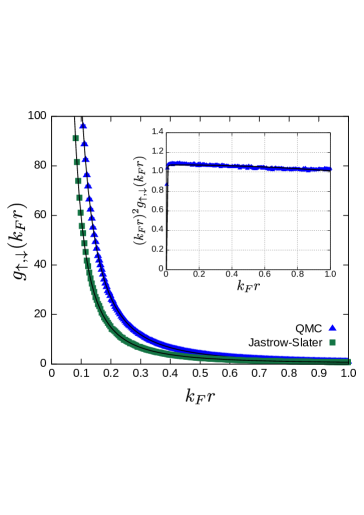
Figure 1: (Color online) Pair distribution function of unlike-spin pairs as a function of the distance. Our quantum Monte Carlo (QMC) results are for a system with 66 particles. The solid line is the best fit of $b_{0}+b/(k_{F}r)^{2}$ to the extrapolated points. For completeness we have included results for the Jastrow-Slater model for a non superfluid system of particles Pessoa et al. (2015). The inset presents the same distributions multiplied by $(k_{F}r)^{2}$ as a function of the distance.

The relation between the constant $\zeta$ and the contact parameter at unitarity is simple, $C/k_{F}^{4}=2\zeta/5\pi$ Gandolfi et al. (2011). However to make the comparison with experimental data easy, we report this quantity in terms of the contact per unit volume given by $\mathcal{C}/Nk_{F}=3\pi^{2}C/k_{F}^{4}$. Our result, $\mathcal{C}$=2.848(1), is slightly below two recent measurements. A Bragg spectroscopy experiment Hoinka et al. (2013) gives the value 3.06 $\pm$ 0.08 at the temperature $T/T_{F}=0.08$. A measurement using radio-frequency spectroscopy gives 2.9 $\pm$ 0.3 at $(k_{F}a)^{-1}=-0.08$ and $T/T_{F}=0.18(2)$, a temperature slightly above the transition temperature $T_{c}$ Sagi et al. (2015). Our computed value is closer to the experimental values than previous results determined with a finite range potential Gandolfi et al. (2011).

The contact $C$ remarkably controls short-distance correlations. On the other hand, the momentum distribution $n_{\sigma}(k)$ in the spin state $\sigma$ for large enough momenta is given by $n_{\sigma}(k)=C/k^{4}$. We have computed the quantity $n(k/k_{F})(k/k_{F})^{4}$ as a function of $k/k_{F}$, and our results are shown in Fig. 2. The contact term is dominant for momentum states larger than approximately $1.6k_{F}$, as we can see from the figure. This dominance is expected since $n(k/k_{F})(k/k_{F})^{4}\rightarrow\frac{2}{3\pi^{2}Nk_{F}}\mathcal{C}$. Although the estimated values of $n(k/k_{F})(k/k_{F})^{4}$ are noisy for large momenta, it is possible to observe a trend towards the value of $\mathcal{C}$, estimated from the pair correlation function, and displayed as a solid line. The less than optimal agreement of our results with the experimental data might come from various sources. It might be due to calculations done at zero temperature while the experiments are, of course, done at finite temperature. Other possibilities might include the asymptotic form we have considered for the guide function; it eventually needs to be improved by including more long-range correlations. However it is worthwhile mentioning that other DMC calculations Carlson et al. (2003) would also overestimate the values of $n(k/k_{F})$ at low values of $k$.

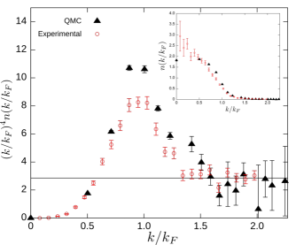
Figure 2: (Color online) Momentum density distribution $n(k/k_{F})$ multiplied by $(k/k_{F})^{4}$ as a function of $k/k_{F}$. In the inset we show $n(k/k_{F})$ as a function of $k/k_{F}$. The solid line shows our estimated value of $\mathcal{C}$. The experimental data is for an inhomogeneous gas Stewart et al. (2010).

IV Summary

In summary, we have performed for the first time diffusion Monte Carlo calculations of a system interacting with a contact interaction. This has allowed us to have a more faithful description of dilute ultracold Fermi gases at unitarity that opens possibilities of more accurate and precise calculations of other important quantities associated with this system. The application of this approach has allowed us to compute such quantities as the reduced chemical potential and Tan’s contact parameter in better agreement with experiment than some previous calculations. We have introduced an alternative way of studying ultracold atoms in the unitary limit which will be of value in the investigation of these systems, and in other situations where a description using a finite effective range interaction might be inaccurate.

Appendix A Sampling the unitary propagator

We will begin by looking at the dominant part of the wave function when an opposite spin pair have a small separation. In this case, we can approximate the trial wave function ratio as

$$\frac{\Psi_{T}(R)}{\Psi_{T}(R^{\prime})}\sim\frac{r^{\prime}}{r}$$ (20)

Since the propagator consists of the free particle gaussian in all channels except the s-wave, we separate it into the usual spherical coordinates $r$, $\cos\theta$, and $\phi$. Starting with the free particle propagator, we take the $z$ axis along the initial value $\bm{r}^{\prime}$ (note we use primed coordinate for the initial value here for convenience; in the main text the initial coordinates are unprimed and the sampled coordinates are primed), and write the importance sampled gaussian as

$$\frac{r^{\prime}}{r}\frac{1}{(2\pi\sigma^{2})^{3/2}}e^{-\frac{|\bm{r}-\bm{r}^{\prime}|^{2}}{2\sigma^{2}}}=\frac{r^{\prime}}{r}\frac{1}{(2\pi\sigma^{2})^{3/2}}e^{-\frac{r^{2}+r^{\prime 2}}{2\sigma^{2}}}e^{\frac{rr^{\prime}}{\sigma^{2}}\cos\theta}\,.$$ (21)

Normalizing the $\cos\theta$ part

$$\int_{-1}^{1}d\cos\theta e^{\frac{rr^{\prime}}{\sigma^{2}}\cos\theta}=\frac{2\sigma^{2}}{rr^{\prime}}\sinh\left(\frac{rr^{\prime}}{\sigma^{2}}\right)$$ (22)

given an $r$ and $r^{\prime}$ value, we can sample the angular part from

$$p_{\phi}(\phi) = \frac{1}{2\pi}$$

$$p_{\theta}(\cos\theta) = \frac{rr^{\prime}}{2\sigma^{2}\sinh\left(\frac{rr^{\prime}}{\sigma^{2}}\right)}e^{\frac{rr^{\prime}}{\sigma^{2}}\cos\theta}\,.$$ (23)

Once we know $r$, we can sample $\cos\theta$ by sampling a uniform random number $0<\xi<1$ and

$$\cos\theta=1+\frac{\sigma^{2}}{rr^{\prime}}\ln\left[\xi\left(1-e^{-\frac{2rr^{\prime}}{\sigma^{2}}}\right)+e^{-\frac{2rr^{\prime}}{\sigma^{2}}}\right]$$ (24)

The importance sampled gaussian is now

$$\frac{r^{\prime}}{r}\frac{1}{(2\pi\sigma^{2})^{3/2}}e^{-\frac{|\bm{r}-\bm{r}^{\prime}|^{2}}{2\sigma^{2}}}=p_{\phi}(\phi)p_{\theta}(\cos\theta)\frac{1}{\sqrt{2\pi}\sigma r^{2}}\left[e^{-\frac{(r-r^{\prime})^{2}}{2\sigma^{2}}}-e^{-\frac{(r+r^{\prime})^{2}}{2\sigma^{2}}}\right]\,.$$ (25)

The integral of the $r$ part over $r^{2}dr$ is

$$\int_{0}^{\infty}dr\frac{1}{\sqrt{2\pi}\sigma}\left[e^{-\frac{(r-r^{\prime})^{2}}{2\sigma^{2}}}-e^{-\frac{(r+r^{\prime})^{2}}{2\sigma^{2}}}\right]={\rm erf}\left(\frac{r^{\prime}}{\sigma\sqrt{2}}\right)\,.$$ (26)

We now look at the “extra” piece from the unitary s-wave interaction. It has the importance sampled form

$$\frac{r^{\prime}}{r}\frac{\sqrt{2\pi}}{4\pi^{2}\sigma rr^{\prime}}e^{-\frac{(r+r^{\prime})^{2}}{2\sigma^{2}}}\,.$$ (27)

Here the angular part is isotropic, so we can sample the angles from

$$p_{\phi}(\phi) = \frac{1}{2\pi}$$

$$p^{(0)}_{\theta}(\cos\theta) = \frac{1}{2}$$ (28)

and the importance sampled function becomes

$$\frac{r^{\prime}}{r}\frac{\sqrt{2\pi}}{4\pi^{2}\sigma rr^{\prime}}e^{-\frac{(r+r^{\prime})^{2}}{2\sigma^{2}}}=p_{\phi}(\phi)p^{(0)}_{\theta}(\cos\theta)\sqrt{\frac{2}{\pi}}\frac{1}{\sigma r^{2}}e^{-\frac{(r+r^{\prime})^{2}}{2\sigma^{2}}}$$ (29)

The integral of the $r$ part over $r^{2}dr$ is

$$\int_{0}^{\infty}dr\sqrt{\frac{2}{\pi}}\frac{1}{\sigma}e^{-\frac{(r+r^{\prime})^{2}}{2\sigma^{2}}}=1-{\rm erf}\left(\frac{r^{\prime}}{\sigma\sqrt{2}}\right)\,.$$ (30)

When we add the normalizations of Eqs. 26 and 30, we get one, since we should get $e^{-E_{0}\tau}$, and with the ground-state energy $E_{0}=0$ since there is no bound state for the unitary gas.

This suggests a way to sample the propagator. We first sample the $r$ value, with probability that the $r$ value was sampled from the gaussian we sample $\cos\theta$ from $p_{\theta}(\cos\theta)$, otherwise, we sample $\cos\theta$ uniformly. In either case, we sample $\phi$ uniformly.

The basic idea below is to sample from a 1-dimensional gaussian centered at $r^{\prime}$. This corresponds to the first term of $g_{s}$. If the resulting $r$ is greater than zero, then it is a legal value. With probability given by the ratio of the radial part of $G_{0}$ divided by the sampled 1-dimensional gaussian, we take this $r$ as being sampled from $G_{0}$, and sample $\cos\theta$ accordingly. If not, the rejected terms have been sampled from the $e^{-\frac{(r+r^{\prime})^{2}}{2\sigma^{2}}}$, so they are half of the s-wave term. If the resulting sampled $r$ is negative, we take its absolute value and it is also sampled from the s-wave term.

Our algorithm is

• Sample a $\phi$ uniformly on $0<\phi<2\pi$ or equivalent.

• Sample a random variate $y$ from a gaussian with mean zero and variance 1.

• The $r$ sample is $r=|r^{\prime}+\sigma y|$.

• If $(r^{\prime}+\sigma y)\leq 0$ sample $\cos\theta$ uniformly. The sampling is complete.

• If $(r^{\prime}+\sigma y)>0$ then sample a random variate $0<\xi<1$ uniformly.

• If $\xi<e^{-\frac{2rr^{\prime}}{\sigma^{2}}}$ sample $\cos\theta$ uniformly, else sample $\cos\theta$ from $p_{\theta}(\cos\theta)$.

A graph of the various terms is shown in fig. 3.

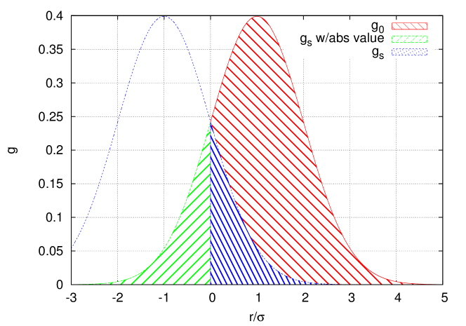
Figure 3: (Color online) The sampling of the radial part of the propagator is illustrated. We sample from the gaussian centered around $r^{\prime}$, in this case taken to be $\sigma$. The probability of this being from the free gaussian is shown as the (red) $g_{0}$ region. It is the difference between the sampled gaussian and the gaussian centered around $-r^{\prime}$, also shown. The (blue) $g_{s}$ region is half the probability of sampling from the s-wave propagator. If we take the absolute value of the sampled value when it is negative, the samples are from the (green) $g_{s}$ w/abs region which gives the other half of the s-wave propagator.

References

- Chin et al. (2010) C. Chin, R. Grimm, P. Julienne, and E. Tiesinga, Reviews of Modern Physics 82, 1225 (2010).
- Giorgini et al. (2008) S. Giorgini, L. P. Pitaevskii, and S. Stringari, Rev. Mod. Phys. 80, 1215 (2008).
- Weimer et al. (2015) W. Weimer, K. Morgener, V. P. Singh, J. Siegl, K. Hueck, N. Luick, L. Mathey, and H. Moritz, Physical Review Letters 114 (2015), 10.1103/physrevlett.114.095301.
- Ferrier-Barbut et al. (2014) I. Ferrier-Barbut, M. Delehaye, S. Laurent, A. T. Grier, M. Pierce, B. S. Rem, F. Chevy, and C. Salomon, Science 345, 1035 (2014), arXiv:1404.2548 [cond-mat.quant-gas] .
- Sidorenkov et al. (2013) L. A. Sidorenkov, M. K. Tey, R. Grimm, Y.-H. Hou, L. Pitaevskii, and S. Stringari, Nature (London) 498, 78 (2013).
- Forbes et al. (2012) M. M. Forbes, S. Gandolfi, and A. Gezerlis, Phys. Rev. A 86, 053603 (2012), arXiv:1205.4815 [cond-mat.quant-gas] .
- Carlson et al. (2003) J. Carlson, S.-Y. Chang, V. R. Pandharipande, and K. E. Schmidt, Phys. Rev. Lett. 91, 050401 (2003).
- Astrakharchik et al. (2004) G. E. Astrakharchik, J. Boronat, J. Casulleras, and S. Giorgini, Phys. Rev. Lett. 93, 200404 (2004).
- Lobo et al. (2006) C. Lobo, A. Recati, S. Giorgini, and S. Stringari, Physical Review Letters 97, 200403 (2006), cond-mat/0607730 .
- Gandolfi et al. (2011) S. Gandolfi, K. E. Schmidt, and J. Carlson, Phys. Rev. A 83, 041601 (2011).
- Bugnion et al. (2014) P. O. Bugnion, P. López Ríos, R. J. Needs, and G. J. Conduit, Phys. Rev. A 90, 033626 (2014), arXiv:1407.0040 [cond-mat.quant-gas] .
- Chang et al. (2011) S.-Y. Chang, M. Randeria, and N. Trivedi, Proceedings of the National Academy of Science 108, 51 (2011).
- Pilati et al. (2010) S. Pilati, G. Bertaina, S. Giorgini, and M. Troyer, Physical Review Letters 105, 030405 (2010), arXiv:1004.1169 [cond-mat.quant-gas] .
- Rossi et al. (2014) M. Rossi, L. Salasnich, F. Ancilotto, and F. Toigo, Phys. Rev. A 89 (2014), 10.1103/physreva.89.041602.
- Bertaina et al. (2013) G. Bertaina, E. Fratini, S. Giorgini, and P. Pieri, Physical Review Letters 110 (2013), 10.1103/physrevlett.110.115303.
- Foulkes et al. (2001) W. M. C. Foulkes, L. Mitas, R. J. Needs, and G. Rajagopal, Rev. Mod. Phys. 73, 33 (2001).
- Chang et al. (2004) S. Y. Chang, V. R. Pandharipande, J. Carlson, and K. E. Schmidt, Physical Review A (Atomic, Molecular, and Optical Physics) 70, 043602 (2004).
- Pessoa et al. (2015) R. Pessoa, S. A. Vitiello, and K. E. Schmidt, J Low Temp Phys 180, 168–179 (2015).
- Sorella (2001) S. Sorella, Phys. Rev. B 64 (2001), 10.1103/physrevb.64.024512.
- Yan and Blume (2015) Y. Yan and D. Blume, Phys. Rev. A 91, 043607 (2015).
- Carlson et al. (2012) J. Carlson, S. Gandolfi, and A. Gezerlis, Progress of Theoretical and Experimental Physics 2012 (2012), 10.1093/ptep/pts031, http://ptep.oxfordjournals.org/content/2012/1/01A209.full.pdf+html .
- Carlson et al. (2015) J. Carlson, S. Gandolfi, F. Pederiva, S. C. Pieper, R. Schiavilla, K. E. Schmidt, and R. B. Wiringa, Rev. Mod. Phys. 87, 1067–1118 (2015).
- Ku et al. (2012) M. J. H. Ku, A. T. Sommer, L. W. Cheuk, and M. W. Zwierlein, Science 335, 563 (2012), arXiv:1110.3309 [cond-mat.quant-gas] .
- Zürn et al. (2013) G. Zürn, T. Lompe, A. N. Wenz, S. Jochim, P. S. Julienne, and J. M. Hutson, Physical Review Letters 110, 135301 (2013), arXiv:1211.1512 [cond-mat.quant-gas] .
- Forbes et al. (2011) M. M. Forbes, S. Gandolfi, and A. Gezerlis, Physical Review Letters 106, 235303 (2011), arXiv:1011.2197 [cond-mat.quant-gas] .
- Carlson et al. (2011) J. Carlson, S. Gandolfi, K. E. Schmidt, and S. Zhang, Phys. Rev. A 84, 061602 (2011).
- Tan (2008a) S. Tan, Annals of Physics 323, 2952 (2008a).
- Tan (2008b) S. Tan, Annals of Physics 323, 2971 (2008b).
- Tan (2008c) S. Tan, Annals of Physics 323, 2987 (2008c).
- Zhang and Leggett (2009) S. Zhang and A. J. Leggett, Phys. Rev. A 79, 023601 (2009), arXiv:0809.1892 [cond-mat.str-el] .
- Hoinka et al. (2013) S. Hoinka, M. Lingham, K. Fenech, H. Hu, C. J. Vale, J. E. Drut, and S. Gandolfi, Physical Review Letters 110, 055305 (2013), arXiv:1209.3830 [cond-mat.quant-gas] .
- Sagi et al. (2015) Y. Sagi, T. E. Drake, R. Paudel, R. Chapurin, and D. S. Jin, Physical Review Letters 114, 075301 (2015), arXiv:1409.4743 [cond-mat.quant-gas] .
- Stewart et al. (2010) J. T. Stewart, J. P. Gaebler, T. E. Drake, and D. S. Jin, Physical Review Letters 104, 235301 (2010), arXiv:1002.1987 [cond-mat.quant-gas] .