Perturbations of the asymptotic region of the Schwarzschild-de Sitter spacetime

Abstract

The conformal structure of the Schwarzschild-de Sitter spacetime is analysed using the extended conformal Einstein field equations. To this end, initial data for an asymptotic initial value problem for the Schwarzschild-de Sitter spacetime is obtained. This initial data allows to understand the singular behaviour of the conformal structure at the asymptotic points where the horizons of the Schwarzschild-de Sitter spacetime meet the conformal boundary. Using the insights gained from the analysis of the Schwarzschild-de Sitter spacetime in a conformal Gaussian gauge, we consider nonlinear perturbations close to the Schwarzschild-de Sitter spacetime in the asymptotic region. We show that small enough perturbations of asymptotic initial data for the Schwarzschild de-Sitter spacetime give rise to a solution to the Einstein field equations which exists to the future and has an asymptotic structure similar to that of the Schwarzschild-de Sitter spacetime.

Keywords: Conformal methods, spinors, black holes, Schwarzschild-de Sitter spacetime, global existence.

PACS: 04.20.Ex, 04.20.Ha, 04.20.Gz

1 Introduction

The stability of black hole spacetimes is, arguably, one of the outstanding problems in mathematical General Relativity. The challenge in analysing the stability of black hole spacetimes lies in both the mathematical problems as well as in the physical concepts to be grasped. By contrast, the nonlinear stability of Minkowski spacetime —see e.g. [8, 18]— and de Sitter spacetimes —see [16, 18]— are well understood.

The results in [16, 18] show that the so-called conformal Einstein field equations are a powerful tool for the analysis of the stability and global properties of vacuum asymptotically simple spacetimes —see [11, 16, 18, 26]. They provide a system of field equations for geometric objects defined on a 4-dimensional Lorentzian manifold $(\mathcal{M},{\bm{g}})$, the so-called unphysical spacetime, which is conformally related to a spacetime $(\tilde{\mathcal{M}},\tilde{{\bm{g}}})$, the so-called physical spacetime, satisfying the Einstein field equations. The conformal framework allows to recast global problems in $(\tilde{\mathcal{M}},\tilde{{\bm{g}}})$ as local problems in $(\mathcal{M},{\bm{g}})$. The metrics ${\bm{g}}$ and $\tilde{{\bm{g}}}$ are related to each other via a rescaling of the form ${\bm{g}}=\Xi^{2}\tilde{{\bm{g}}}$ where $\Xi$ is a so-called conformal factor. Crucially, the conformal Einstein field equations are regular at the points where $\Xi=0$ —the so-called conformal boundary. Moreover, a solution thereof implies, wherever $\Xi\neq 0$, a solution to the Einstein field equations.

At its core, the conformal Einstein field equations constitute a system of differential conditions on the curvature tensors respect to the Levi-Civita connection of ${\bm{g}}$ and the conformal factor $\Xi$. The original formulation of the equations as given in, say [11, 13], requires the introduction of so-called gauge source functions. An alternative approach to gauge fixing is to adapt the analysis to a congruence of curves. In the context of conformal methods, a natural candidate for a congruence is given by conformal geodesics —see [28, 24]. To combine gauges based on the properties of congruences of conformal geodesics with the conformal Einstein field equations, one needs a more general version of the latter —the so-called extended conformal Einstein field equations [20]. The extended conformal field equations have been used to obtain an alternative proof of the semiglobal nonlinear stability of the Minkowski spacetime and of the global nonlinear stability of the de-Sitter spacetime —see [40]. In view of these results, a natural question is whether conformal methods can be used in the global analysis of spacetimes containing black holes. This article gives a first step in this direction by analysing certain aspects of the conformal structure of the Schwarzschild-de Sitter spacetime.

1.1 The Schwarzschild-de Sitter spacetime

The Schwarzschild-de Sitter spacetime is a spherically symmetric solution to the vacuum Einstein field equations with Cosmological constant. It depends on two parameters: the Cosmological constant $\lambda$ and the mass parameter $m$. The assumption of spherical symmetry almost completely singles out the Schwarzschild-de Sitter spacetime among the vacuum solutions to the Einstein field equations with de Sitter-like Cosmological constant. The other admissible solution is the so-called Nariai spacetime. This observation can be regarded as a generalisation of Birkhoff’s theorem —see [50]. For small values of the areal radius $r$, the solution behaves like the Schwarzschild spacetime and for large values its behaviour resembles that of the de Sitter spacetime. In the Schwarzschild-de Sitter spacetime the relation between the mass and Cosmological constant determines the location of the Cosmological and black hole horizons.

The presence of a Cosmological constant makes the Schwarzschild-de Sitter solution a convenient candidate for a global analysis by means of the extended conformal field equations: the solution is an example of a spacetime which admits a smooth conformal extension towards the future (respectively, the past) —see Figures 3, 4 and 5 in the main text. This type of spacetimes are called future (respectively, past) asymptotically de Sitter —see Section 2.1 for definitions and [1, 29] for a more extensive discussion. As the Cosmological constant takes a de Sitter-like value, the conformal boundary of the spacetime is spacelike and, moreover, there exists a conformal representation in which the induced 3-metric on the conformal boundary $\mathscr{I}$ is homogeneous. Thus, it is possible to integrate the extended conformal field equations along single conformal geodesics.

In this article we analyse the Schwarzschild-de Sitter spacetime as a solution to the extended conformal Einstein field equations and use the insights thus obtained to discuss nonlinear perturbations of the spacetime. A natural starting point for this discussion is the analysis of conformal geodesic equations on the spacetime. The results of this analysis can, in turn, be used to rewrite the spacetime in the conformal gauge associated to these curves. However, despite the fact that the conformal geodesic equations for spherically symmetric spacetimes can be written in quadratures [24], in general, the integrals involved cannot be solved analytically. In view of this difficulty, in this article we analyse the conformal properties of the exact Schwarzschild-de Sitter spacetime by means of an asymptotic initial value problem for the conformal field equations. Accordingly, we compute the initial data implied by the Schwarzschild-de Sitter spacetime on the conformal boundary and then use it to analyse the behaviour of the conformal evolution equations. An important property of these evolution equations is that their essential dynamics is governed by a core system. Consequently, an important aspect of our discussion consists of the analysis of the formation of singularities in the core system. This analysis is irrespective of the relation between $\lambda\neq 0$ and $m$. This allows us to formulate a result which is valid for the subextremal, extremal and hyperextremal Schwarzschild-de Sitter spacetime characterised by the conditions $0<9m^{2}|\lambda|<1$, $9m^{2}|\lambda|=1$ and $9m^{2}|\lambda|>1$ respectively.

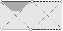
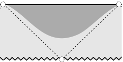
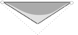
Figure 1: Schematic depiction of the Main Result. Development of asymptotic initial data close to that of the Schwarzschild-de Sitter spacetime in the global representation —the initial metric is $\bm{\hbar}$, the standard metric on $\mathbb{S}^{3}$, and the asymptotic points $\mathcal{Q}$ and $\mathcal{Q^{\prime}}$ are excluded (denoted by empty circles in the diagram). Figures a), b) and c) illustrate the evolution of initial data close to the Schwarzschild-de Sitter spacetime in the subextremal, extremal and hyperextremal cases respectively. See also Figures 3,4 and 5.

Figure 2: Schematic depiction of the Main Result. Development of asymptotic initial data close to that of the Schwarzschild-de Sitter spacetime in the representation in which Theorem 1 was obtained. The initial metric is ${\bm{h}}$, the standard metric on $\mathbb{R}\times\mathbb{S}^{2}$, and the asymptotic points $\mathcal{Q}$ and $\mathcal{Q^{\prime}}$ are at infinity respect to ${\bm{h}}$ —since ${\bm{\hbar}}$ and ${\bm{h}}$ are conformally flat one has ${\bm{h}}=\omega^{2}{\bm{\hbar}}$. The initial data for the subextremal, extremal and hyperextremal cases is formally identical. Small enough perturbations the development has the same asymptotic structure as the reference spacetime

1.2 The main result

The analysis of the conformal properties of the Schwarzschild-de Sitter spacetime allows us to formulate a result concerning the existence of solutions to the asymptotic initial value problem for the Einstein field equations with de Sitter-like Cosmological constant which can be regarded as perturbations of the asymptotic region of the Schwarzschild-de Sitter spacetime —see Figures 1 and 2. Our existence result can be stated as:

Main Result (asymptotically de Sitter spacetimes close to the asymptotic region of the SdS spacetime).

Given asymptotic initial data which is suitably close to data for the Schwarzschild-de Sitter spacetime there exists a solution to the Einstein field equations which exists towards the future (past) and has an asymptotic structure similar to that of the Schwarzschild-de Sitter spacetime —that is, the solution is future (past) asymptotically de Sitter.

Remark 1.

A detailed formulation of the Main Result of this article can be found in Section 4.4 —see Theorem 1.

Our analysis of the conformal evolution equations governing the dynamics of the background solution provides explicit minimal existence intervals for the solutions. These intervals are certainly not optimal. An interesting question related to the class of solutions to the Einstein field equations obtained in this article is to obtain their maximal development. To address this problem one requires different methods of the theory of partial differential equations and it will be discussed elsewhere. A schematic depiction of the Main Result is given in Figure 1.

As part of the analysis of the background solution we require asymptotic initial data for the Schwarzschild-de Sitter spacetime. The construction of this initial data allows to study in detail the singular behaviour of the conformal structure of the family of background spacetimes at the asymptotic points $\mathcal{Q}$ and $\mathcal{Q}^{\prime}$, where the horizons of the spacetime meet the conformal boundary. As a consequence of the singular behaviour of the asymptotic initial data, the discussion of the asymptotic initial value problem has to exclude these points. In view of this, it turns out that a more convenient conformal representation to analyse the conformal evolution equations for both the exact Schwarzschild-de Sitter spacetime and its perturbations is one in which the the conformal boundary is metrically $\mathbb{R}\times\mathbb{S}^{2}$ rather than $\mathbb{S}^{3}\backslash\{\mathcal{Q},\mathcal{Q^{\prime}}\}$ so that the problematic asymptotic points are sent to infinity —see Figure 2. In this representation, the methods of the theory of partial differential equations used to analyse the existence of solutions to the conformal evolution equations implicitly impose some decay conditions at infinity on the perturbed initial data.

1.3 Related results

The properties of the Schwarzschild-de Sitter spacetime have been systematically probed by means of an analysis of the solutions of the scalar wave equation using vector field methods —see [48]. This type of analysis requires special care when discussing the behaviour of the solution close to the horizons. In the asymptotic initial value problem considered in this article, the domain of influence of the initial data is contained in the region corresponding to the asymptotic region of the Schwarzschild-de Sitter spacetime.

The properties of the Nariai spacetime —the other solution appearing in the generalisation of Birkhoff’s theorem to spacetimes with a de Sitter-like Cosmological constant— have been analysed by means of both analytic and numerical methods in [5, 6]. In particular, in the former reference it is shown that the Nariai solution does not admit a smooth conformal extension —see also [26]. Thus, it cannot be obtained from an asymptotic initial value problem.

Finally, it is pointed out that the singularity of the Schwarzschild-de Sitter spacetime is not a conformal gauge singularity since $\tilde{C}_{abcd}\tilde{C}^{abcd}\rightarrow\infty$ as $r\rightarrow 0$. Accordingly, theory of the extendibility of conformal gauge singularities as developed in [39] cannot be applied to our analysis. For any of the possible conformal gauges available, one either has a singularity of the Weyl tensor arising at a finite value of the parameter of a conformal geodesic or one has an inextendible conformal geodesic along which the Weyl tensor is always smooth.

Notations and conventions

The signature convention for (Lorentzian) spacetime metrics is $(+,-,-,-)$. In these conventions the Cosmological constant $\lambda$ of the de Sitter spacetime takes negative values. Cosmological constants with negative values will be said to be de Sitter-like.

In what follows, the Latin indices ${}_{a},\,{}_{b},{}_{c},\,\ldots$ are used as abstract tensor indices while the boldface Latin indices ${}_{\bm{a}},\,{}_{\bm{b}},{}_{\bm{c}},\ldots$ are used as spacetime frame indices taking the values $0,\ldots,3$. In this way, given a basis $\{{\bm{e}}_{{\bm{a}}}\}$ a generic tensor is denoted by $T_{ab}$ while its components in the given basis are denoted by $T_{{\bm{a}}{\bm{b}}}\equiv T_{ab}{\bm{e}}_{{\bm{a}}}{}^{a}{\bm{e}}_{{\bm{b}}}{}^{b}$. We reserve the indices ${}_{\bm{i}},\,{}_{\bm{j}},\,{}_{\bm{k}},\ldots$ to denote frame spatial indices respect to an adapted frame taking the values $1,\,2,\,3$. We make systematic use of spinors and follow the conventions and notation of Penrose & Rindler [45] —in particular, ${}_{A},\,{}_{B},\,{}_{C},\ldots$ are abstract spinorial indices while ${}_{\bm{A}},\,{}_{\bm{B}},\,{}_{\bm{C}},\ldots$ will denote frame spinorial indices with respect to some specified spin dyad $\{\epsilon_{\bm{A}}{}^{A}\}$. Our conventions for the curvature tensors are fixed by the relation:

$$(\nabla_{a}\nabla_{b}-\nabla_{b}\nabla_{a})v^{c}=R^{c}{}_{dab}v^{d}.$$

In addition, $D^{\pm}(\mathcal{A})$, $H(\mathcal{A})$, $J^{\pm}(\mathcal{A})$ and $I^{\pm}(\mathcal{A})$ will denote, respectively, the future (past) domain of dependence, the Cauchy horizon, the causal and the chronological futures (pasts) of $\mathcal{A}$ —see e.g. [36, 55].

2 The asymptotic initial value problem in General Relativity

In this section we briefly revisit the notion of asymptotically de Sitter spacetimes —see [1, 29, 36]. After that, we review the properties of the extended conformal Einstein field equations that will be used in our analysis of the Schwarzschild-de Sitter spacetime. This general conformal representation of the Einstein field equations was originally introduced in [20] —see also [25, 52, 53] for further discussion. For completeness, the conformal constraint equations are presented —see [13, 14, 17, 25]. In addition, we provide a discussion on the notion of conformal geodesics and conformal Gaussian systems of coordinates —see [49, 28, 24, 20]. In this section we also discuss how to use the conformal field equations expressed in terms of a conformal Gaussian system to set up an asymptotic initial value problem for a spacetime with a spacelike conformal boundary. We conclude this section with a discussion of the structural properties of the conformal evolution equations in the framework of the theory of symmetric hyperbolic systems contained in [37].

2.1 Asymptotically de Sitter spacetimes

A spacetime $(\tilde{\mathcal{M}},\tilde{{\bm{g}}})$ satisfying the vacuum Einstein field equations

$$\tilde{R}_{ab}=\lambda\tilde{g}_{ab},$$ (1)

is future asymptotically de Sitter if there exist a spacetime with boundary $(\mathcal{M},{\bm{g}})$, a smooth conformal factor $\Xi$ and a diffeomorphism $\varphi:\tilde{\mathcal{M}}\rightarrow\mathcal{U}\subseteq\mathcal{M}$, such that:

$$\Xi>0\qquad\text{in}\qquad\mathcal{U},$$

$$\Xi=0\quad\text{and}\quad\textbf{\mbox{d}}\Xi\neq 0\quad\text{on}\quad\mathscr{I}^{+}\equiv\partial{\mathcal{U}},$$

$$\mathscr{I}^{+}\quad\text{is spacelike ---i.e. }\quad{\bm{g}}(\textbf{\mbox{d}}\Xi,\textbf{\mbox{d}}\Xi)>0\qquad\text{on}\qquad\mathscr{I}^{+},$$

$$\mathscr{I}^{+}\quad\text{lies to the future of }\tilde{\mathcal{M}}\quad\mbox{---i.e.}\quad\mathscr{I}^{+}\subset I^{+}(\tilde{\mathcal{M}}).$$

Observe that this definition does not restrict the topology of $\mathscr{I}^{+}$. In particular, it does not have to be compact —see [29]. The notion of past asymptotically de Sitter is defined in analogous way. Additionally, $(\tilde{\mathcal{M}},\tilde{{\bm{g}}})$ is asymptotically de Sitter if it is future and past asymptotically de Sitter. Notice that a spacetime which is asymptotically de Sitter is not necessarily asymptotically simple —see [36] for a precise definition of asymptotically simple spacetime. In the following, in a slight abuse of notation, the mapping $\varphi:\tilde{\mathcal{M}}\rightarrow\mathcal{U}\subseteq\mathcal{M}$ will be omitted in the notation and we write

$${\bm{g}}=\Xi^{2}\tilde{{\bm{g}}}.$$ (2)

Furthermore, the term asymptotic region will be used to refer to the set $J^{-}(\mathscr{I}^{+})$ of a future asymptotically de Sitter spacetime or $J^{+}(\mathscr{I}^{-})$ of a past asymptotically de Sitter spacetime.

2.2 The extended conformal Einstein field equations

In this section we provide a succinct discussion of the extended conformal Einstein field equations.

2.2.1 Basic notions

Given any connection ${\bm{\nabla}}$ over a spacetime manifold $\tilde{\mathcal{M}}$, the torsion and Riemann curvature tensors are defined, respectively, by the expressions

$$(\nabla_{a}\nabla_{b}-\nabla_{b}\nabla_{a})\phi=\Sigma_{a}{}^{c}{}_{b}\nabla_{c}\phi,\qquad\qquad(\nabla_{a}\nabla_{b}-\nabla_{b}\nabla_{a})u^{c}=R^{c}{}_{dab}u^{d}+\Sigma_{a}{}^{d}{}_{b}\nabla_{d}u^{c},$$

where $\phi$ and $u^{d}$ are smooth scalar and vector fields respectively, while $\Sigma_{a}{}^{c}{}_{b}$ and $R^{d}{}_{cab}$ denote the torsion and Riemann tensors of ${\bm{\nabla}}$.

2.2.2 Frames and connection coefficients

Let $\{{\bm{e}}_{{\bm{a}}}\}$ denote a set of frame fields on $\tilde{\mathcal{M}}$ and let $\{{\bm{\omega}}^{\bm{a}}\}$ be the associated coframe. One has that $\langle\omega^{\bm{a}},{\bm{e}}_{\bm{b}}\rangle=\delta_{\bm{b}}{}^{\bm{a}}$. We define the frame metric as $g_{{\bm{a}}{\bm{b}}}\equiv{\bm{g}}({\bm{e}}_{{\bm{a}}},{\bm{e}}_{{\bm{b}}})$ —in abstract index notation $g_{{\bm{a}}{\bm{b}}}\equiv{\bm{e}}_{{\bm{a}}}{}^{a}{\bm{e}}_{{\bm{b}}}{}^{b}g_{ab}$. From now on we will restrict our attention to orthonormal frames, so that $g_{{\bm{a}}{\bm{b}}}=\eta_{{\bm{a}}{\bm{b}}}$, where consistent with our signature conventions $\eta_{{\bm{a}}{\bm{b}}}=\text{diag}(1,-1,-1,-1)$. The metric ${\bm{g}}$ is then expressed in terms of the coframe $\{{\bm{\omega}}^{\bm{a}}\}$ as

$${\bm{g}}=\eta_{{\bm{a}}{\bm{b}}}{\bm{\omega}}^{\bm{a}}\otimes{\bm{\omega}}^{\bm{b}}.$$

The connection coefficients $\Gamma_{{\bm{a}}}{}^{{\bm{c}}}{}_{{\bm{b}}}$ of the connection ${\bm{\nabla}}$ with respect to the frame $\{{\bm{e}}_{\bm{a}}\}$ are defined via the relation

$$\nabla_{{\bm{a}}}{\bm{e}}_{{\bm{b}}}=\Gamma_{{\bm{a}}}{}^{{\bm{c}}}{}_{{\bm{b}}}{\bm{e}}_{{\bm{c}}},$$

where $\nabla_{{\bm{a}}}\equiv{\bm{e}}_{{\bm{a}}}{}^{a}\nabla_{a}$ denotes the covariant directional derivative in the direction of ${\bm{e}}_{{\bm{a}}}$. The torsion of ${\bm{\nabla}}$ can be expressed in terms of the frame $\{{\bm{e}}_{{\bm{a}}}\}$ and the connection coefficients $\Gamma_{{\bm{a}}}{}^{{\bm{c}}}{}_{{\bm{b}}}$ via

$$\Sigma_{{\bm{a}}}{}^{{\bm{c}}}{}_{{\bm{b}}}{\bm{e}}_{{\bm{c}}}=[{\bm{e}}_{{\bm{a}}},{\bm{e}}_{{\bm{b}}}]-(\Gamma_{{\bm{a}}}{}^{{\bm{c}}}{}_{{\bm{b}}}-\Gamma_{{\bm{b}}}{}^{{\bm{c}}}{}_{{\bm{a}}}){\bm{e}}_{{\bm{c}}}.$$

2.2.3 Conformal rescalings

Following the notation introduced in Section 2.1, two spacetimes $(\mathcal{M},{\bm{g}})$ are said to be $(\tilde{\mathcal{M}},\tilde{{\bm{g}}})$ conformally related if the metrics ${\bm{g}}$ and $\tilde{{\bm{g}}}$ satisfy equation (2) for some scalar field $\Xi$. In the remainder of this article the symbols ${\bm{\nabla}}$ and $\tilde{{\bm{\nabla}}}$ will be reserved for the Levi-Civita connection of the metrics ${\bm{g}}$ and $\tilde{{\bm{g}}}$. The connection coefficients of ${\bm{\nabla}}$ and $\tilde{{\bm{\nabla}}}$ are related to each other through the expression

$$\Gamma_{{\bm{a}}}{}^{{\bm{c}}}{}_{{\bm{b}}}=\tilde{\Gamma}_{{\bm{a}}}{}^{{\bm{c}}}{}_{{\bm{b}}}+S_{{\bm{a}}{\bm{b}}}{}^{{\bm{c}}{\bm{d}}}\Upsilon_{{\bm{d}}},$$

where

$$S_{{\bm{a}}{\bm{b}}}{}^{{\bm{c}}{\bm{d}}}\equiv\delta_{{\bm{a}}}{}^{{\bm{c}}}\delta_{{\bm{b}}}{}^{{\bm{d}}}+\delta_{{\bm{b}}}{}^{{\bm{c}}}\delta_{{\bm{a}}}{}^{{\bm{d}}}-g_{{\bm{a}}{\bm{b}}}g^{{\bm{c}}{\bm{d}}}\qquad\text{and}\qquad\Upsilon_{{\bm{a}}}\equiv\Xi^{-1}\nabla_{{\bm{a}}}\Xi.$$

In particular, observe that the 1-form ${\bm{\Upsilon}}\equiv\Upsilon_{\bm{a}}{\bm{\omega}}^{\bm{a}}$ is exact.

2.2.4 Weyl connections

A Weyl connection $\hat{{\bm{\nabla}}}$ is a torsion-free connection satisfying the relation

$$\hat{\nabla}_{a}g_{bc}=-2f_{a}g_{bc},$$ (3)

where $f_{a}$ is an arbitrary 1-form —thus, $\hat{{\bm{\nabla}}}$ is not necessarily a metric connection. Property (3) is preserved under the conformal rescaling (2) as it can be verified that $\hat{\nabla}_{a}\tilde{g}_{bc}=-2\tilde{f}_{a}\tilde{g}_{bc}$ where $\tilde{f}_{a}\equiv f_{a}+\Upsilon_{a}$. The connection coefficients of $\hat{{\bm{\nabla}}}$ are related to those of ${\bm{\nabla}}$ through the relation

$$\hat{\Gamma}_{{\bm{a}}}{}^{{\bm{c}}}{}_{{\bm{b}}}=\Gamma_{{\bm{a}}}{}^{{\bm{c}}}{}_{{\bm{b}}}+S_{{\bm{a}}{\bm{b}}}{}^{{\bm{c}}{\bm{d}}}f_{{\bm{d}}}.$$ (4)

A Weyl connection is a Levi-Civita connection of some element of the conformal class $[{\bm{g}}]$ if and only if the 1-form $f_{a}$ is exact. The Schouten tensor $L_{ab}$ of the connection ${\bm{\nabla}}$ is defined as

$$L_{ab}\equiv\frac{1}{2}R_{ab}-\frac{1}{12}Rg_{ab}.$$

The Schouten tensors of the connections $\hat{\nabla}$ and $\nabla$ are related to each other by

$$L_{ab}-\hat{L}_{ab}=\nabla_{a}f_{b}-\frac{1}{2}S_{ab}{}^{cd}f_{c}f_{d}$$ (5)

Notice that, in general, $\hat{L}_{ab}\neq\hat{L}_{(ab)}$.

2.2.5 The extended conformal Einstein field equations

From now on, we will consider Weyl connections $\hat{{\bm{\nabla}}}$ related to a conformal metric ${\bm{g}}$ as in equation (3). Let $\hat{P}^{{\bm{a}}}{}_{{\bm{b}}{\bm{c}}{\bm{d}}}$ denote the geometric curvature of $\hat{{\bm{\nabla}}}$ —that is, the expression of the Riemann tensor of $\hat{{\bm{\nabla}}}$ written in terms of derivatives of the connection coefficients $\hat{\Gamma}_{{\bm{a}}}{}^{{\bm{c}}}{}_{{\bm{b}}}$:

$$\hat{P}^{{\bm{a}}}{}_{{\bm{b}}{\bm{c}}{\bm{d}}}\equiv{\bm{e}}_{{\bm{a}}}(\hat{\Gamma}_{{\bm{b}}}{}^{{\bm{c}}}{}_{{\bm{d}}})-{\bm{e}}_{{\bm{b}}}(\hat{\Gamma}_{{\bm{a}}}{}^{{\bm{c}}}{}_{{\bm{d}}})+\hat{\Gamma}_{{\bm{f}}}{}^{{\bm{c}}}{}_{{\bm{d}}}(\hat{\Gamma}_{{\bm{b}}}{}^{{\bm{f}}}{}_{{\bm{a}}}-\hat{\Gamma}_{{\bm{a}}}{}^{{\bm{f}}}{}_{{\bm{b}}})+\hat{\Gamma}_{{\bm{b}}}{}^{{\bm{f}}}{}_{{\bm{d}}}\hat{\Gamma}_{{\bm{a}}}{}^{{\bm{c}}}{}_{{\bm{f}}}-\hat{\Gamma}_{{\bm{a}}}{}^{{\bm{f}}}{}_{{\bm{d}}}\hat{\Gamma}_{{\bm{b}}}{}^{{\bm{c}}}{}_{{\bm{f}}}.$$

The expression of the irreducible decomposition of Riemann tensor $\hat{R}^{{\bm{a}}}{}_{{\bm{b}}{\bm{c}}{\bm{d}}}$ given by

$$\hat{\rho}^{{\bm{a}}}{}_{{\bm{b}}{\bm{c}}{\bm{d}}}\equiv\Xi d^{{\bm{a}}}{}_{{\bm{b}}{\bm{c}}{\bm{d}}}+2S_{{\bm{b}}[{\bm{c}}}{}^{{\bm{a}}{\bm{f}}}{\hat{L}}_{{\bm{b}}]{\bm{f}}}$$ (6)

will be called the algebraic curvature. In the last expression $d^{{\bm{a}}}{}_{{\bm{b}}{\bm{c}}{\bm{d}}}$ represents the so-called rescaled Weyl tensor, defined as

$$d^{{\bm{a}}}{}_{{\bm{b}}{\bm{c}}{\bm{d}}}\equiv\Xi^{-1}C^{{\bm{a}}}{}_{{\bm{b}}{\bm{c}}{\bm{d}}},$$

where $C^{{\bm{a}}}{}_{{\bm{b}}{\bm{c}}{\bm{d}}}$ is the Weyl tensor of the metric ${\bm{g}}$. Despite the fact that the definition of the rescaled Weyl tensor may look singular at the conformal boundary, it can be shown that under suitable assumptions the tensor $d^{a}{}_{bcd}$ it is regular even when $\Xi=0$. Finally, let us introduce a 1-form ${\bm{d}}$ defined by the relation

$$d_{\bm{a}}\equiv\Xi f_{\bm{a}}+\nabla_{\bm{a}}\Xi.$$

With the above definitions one can write the vacuum extended conformal Einstein field equations as

$$\hat{\Sigma}_{{\bm{a}}}{}^{{\bm{c}}}{}_{{\bm{b}}}=0,\qquad\hat{\Xi}^{{\bm{a}}}{}_{{\bm{b}}{\bm{c}}{\bm{d}}}=0,\qquad\hat{\Delta}_{{\bm{c}}{\bm{d}}{\bm{b}}}=0,\qquad\hat{\Lambda}_{{\bm{b}}{\bm{c}}{\bm{d}}}=0$$ (7)

where

$$\hat{\Sigma}_{{\bm{a}}}{}^{{\bm{c}}}{}_{{\bm{b}}}\equiv[{\bm{e}}_{{\bm{a}}},{\bm{e}}_{{\bm{b}}}]-(\hat{\Gamma}_{{\bm{a}}}{}^{{\bm{c}}}{}_{{\bm{b}}}-\hat{\Gamma}_{{\bm{b}}}{}^{{\bm{c}}}{}_{{\bm{a}}}){\bm{e}}_{{\bm{c}}},$$ (8a)

$$\hat{\Xi}^{{\bm{a}}}{}_{{\bm{b}}{\bm{c}}{\bm{d}}}\equiv\hat{P}^{{\bm{a}}}{}_{{\bm{b}}{\bm{c}}{\bm{d}}}-\hat{R}^{{\bm{a}}}{}_{{\bm{b}}{\bm{c}}{\bm{d}}},$$ (8b)

$$\hat{\Delta}_{{\bm{c}}{\bm{d}}{\bm{b}}}\equiv\hat{\nabla}_{{\bm{c}}}\hat{L}_{{\bm{b}}{\bm{d}}}-\hat{\nabla}_{{\bm{d}}}\hat{L}_{{\bm{c}}{\bm{b}}}-d_{{\bm{a}}}d^{{\bm{a}}}{}_{{\bm{b}}{\bm{c}}{\bm{d}}}=0,$$ (8c)

$$\hat{\Lambda}_{{\bm{b}}{\bm{c}}{\bm{d}}}\equiv\hat{\nabla}_{{\bm{a}}}d^{{\bm{a}}}{}_{{\bm{b}}{\bm{c}}{\bm{d}}}-f_{{\bm{a}}}d^{{\bm{a}}}{}_{{\bm{b}}{\bm{c}}{\bm{d}}}.$$ (8d)

The fields $\hat{\Sigma}_{{\bm{a}}}{}^{{\bm{c}}}{}_{{\bm{b}}}$, $\hat{\Xi}^{{\bm{a}}}{}_{{\bm{b}}{\bm{c}}{\bm{d}}}$, $\hat{\Delta}$ and $\hat{\Lambda}_{{\bm{b}}{\bm{c}}{\bm{d}}}$ will be called zero-quantities.

The geometric meaning of the extended conformal field equations is the following: $\hat{\Sigma}_{{\bm{a}}}{}^{{\bm{c}}}{}_{{\bm{b}}}=0$ describes the fact that the connection $\hat{\nabla}$ is torsion-free. The equation $\hat{\Xi}^{{\bm{a}}}{}_{{\bm{b}}{\bm{c}}{\bm{d}}}=0$ expresses the fact that the algebraic and geometric curvature coincide. The equations $\hat{\Delta}_{{\bm{c}}{\bm{d}}{\bm{b}}}=0$ and $\hat{\Lambda}_{{\bm{b}}{\bm{c}}{\bm{d}}}=0$ encode the contracted second Bianchi identity. Observe that there is no differential condition for neither the 1-form ${\bm{d}}$ nor the conformal factor. In Section 2.2.6 it will be discussed how to fix these fields by gauge conditions.

In order to relate the conformal equations (7) to the vacuum Einstein field equations (41) one introduces the constraints

$$\delta_{{\bm{a}}}=0,\qquad\gamma_{{\bm{a}}{\bm{b}}}=0,\qquad\zeta_{{\bm{a}}{\bm{b}}}=0$$ (9)

encoded in the supplementary zero-quantities

$$\delta_{{\bm{a}}}\equiv d_{{\bm{a}}}-\Xi f_{{\bm{a}}}-\hat{\nabla}\Xi,$$

$$\gamma_{{\bm{a}}{\bm{b}}}\equiv\frac{1}{6}\lambda\Xi^{-2}\eta_{{\bm{a}}{\bm{b}}}-\hat{\nabla}_{{\bm{a}}}(\Xi^{-1}d_{{\bm{b}}})-\Xi^{-2}S_{{\bm{a}}{\bm{b}}}{}^{{\bm{c}}{\bm{d}}}d_{{\bm{c}}}d_{{\bm{d}}},$$

$$\zeta_{{\bm{a}}{\bm{b}}}\equiv\hat{L}_{[{\bm{a}}{\bm{b}}]}-\hat{\nabla}_{{\bm{a}}}f_{{\bm{b}}}.$$

The first equation in (9) encodes the definition of the 1-form $d_{{\bm{a}}}$; the second equation in (9) arises from the transformation law between the Schouten tensor $\hat{L}_{{\bm{a}}{\bm{b}}}$ of $\hat{{\bm{\nabla}}}$ and the physical Schouten tensor $\tilde{L}_{{\bm{a}}{\bm{b}}}=\frac{1}{6}\tilde{\eta}_{{\bm{a}}{\bm{b}}}$ determined by the Einstein field equations (41); the last equation in (9) relates the antisymmetry of the Schouten tensor $\hat{L}_{ab}$ to the derivative of the 1-form $f_{a}$.

The precise relation between the extended conformal Einstein field equations and the Einstein field equations is given by the following lemma:

Lemma 1.

Let $({\bm{e}}_{{\bm{a}}}{}^{a},\hat{\Gamma}_{{\bm{a}}}{}^{{\bm{b}}}{}_{{\bm{c}}},\hat{L}_{{\bm{a}}{\bm{b}}},d^{{\bm{a}}}{}_{{\bm{b}}{\bm{c}}{\bm{d}}})$ denote a solution to the vacuum extended conformal Einstein field equations (7) for some choice of gauge fields $(\Xi,d_{{\bm{a}}})$ satisfying the constraint equations (9). Assume, further, that

$$\Xi\neq 0\qquad\text{and}\qquad det(\eta^{{\bm{a}}{\bm{b}}}{\bm{e}}_{{\bm{a}}}{\bm{e}}_{{\bm{b}}})\neq 0$$

on an open subset $\mathcal{U}\subset\tilde{\mathcal{M}}$. Then

$$\tilde{{\bm{g}}}=\Theta^{-2}\eta_{{\bm{a}}{\bm{b}}}{\bm{\omega}}^{{\bm{a}}}\otimes{\bm{\omega}}^{{\bm{b}}},$$

where $\{{\bm{\omega}}^{{\bm{a}}}\}$ is the coframe dual to $\{{\bm{e}}_{{\bm{a}}}\}$, is a solution to the vacuum Einstein field equations (41) on $\mathcal{U}$.

The proof of this lemma can be found in [24, 53].

2.2.6 Conformal geodesics and conformal Gaussian systems

A conformal geodesic on a spacetime $(\tilde{\mathcal{M}},\tilde{{\bm{g}}})$ consists of a pair $(x(\tau),{\bm{\beta}}(\tau))$ where $x(\tau)$ is a curve with tangent $\dot{{\bm{x}}}(\tau)$ and $\bm{\beta}(\tau)$ is a 1-form defined along $x(\tau)$ satisfying the conformal geodesic equations

$$\dot{x}^{c}\tilde{\nabla}_{c}\dot{x}^{a}=-\dot{x}^{d}\dot{x}^{b}S_{db}{}^{af}\beta_{f},$$ (11a)

$$\dot{x}^{c}\tilde{\nabla}_{c}\beta_{a}=-\tfrac{1}{2}\dot{x}^{c}S_{ca}{}^{bd}\beta_{b}\beta_{d}+\tilde{L}_{ca}\dot{x}^{c},$$ (11b)

where $\tilde{L}_{ca}$ denotes the Schouten tensor of $\tilde{\nabla}$ and

$$S_{ab}{}^{cd}\equiv\delta_{a}{}^{c}\delta_{b}{}^{d}+\delta_{a}{}^{d}\delta_{b}{}^{c}-\tilde{g}_{ab}\tilde{g}^{cd}.$$

In addition, it is convenient to consider a Weyl propagated frame —that is, a frame field $\{{\bm{e}}_{{\bm{a}}}{}^{a}\}$ satisfying

$$\dot{x}^{c}\tilde{\nabla}_{c}{\bm{e}}_{{\bm{a}}}{}^{a}=-S_{cd}{}^{af}{\bm{e}}_{{\bm{a}}}{}^{d}\dot{x}^{c}\beta_{f}.$$

The definition of conformal geodesics is motivated by the transformation laws of equations (11a)-(11b) under conformal rescalings and transitions to Weyl connections. More precisely, given an arbitrary 1-form $\wideparen{{\bm{f}}}$ one can construct a Weyl connection $\wideparen{\nabla}$ as in equation (3). Then, defining $\wideparen{{\bm{\beta}}}\equiv{\bm{\beta}}-\wideparen{{\bm{f}}}$ the pair $(x(\tau),\wideparen{{\bm{\beta}}}(\tau))$ will satisfy the equations

$$\dot{x}^{c}\wideparen{\nabla}_{c}\dot{x}^{a}=-\dot{x}^{d}\dot{x}^{b}S_{db}{}^{af}\wideparen{\beta}_{f},$$

$$\dot{x}^{c}\wideparen{\nabla}_{c}\wideparen{\beta}_{a}=-\tfrac{1}{2}\dot{x}^{c}S_{ca}{}^{bd}\wideparen{\beta}_{b}\wideparen{\beta}_{d}+\wideparen{L}_{ca}\dot{x}^{c},$$

where $\wideparen{L}_{ca}$ is the Schouten tensor of the connection $\wideparen{{\bm{\nabla}}}$ as defined in equation (5). If one chooses a Weyl connection $\hat{{\bm{\nabla}}}$ whose defining 1-form ${\bm{f}}$ coincides with the 1-form ${\bm{\beta}}$ of the $\hat{{\bm{\nabla}}}$-conformal geodesic equations (11a)-(11b), then the conformal geodesic equations reduce to

$$\dot{x}^{c}\hat{\nabla}_{c}\dot{x}^{a}=0,\qquad\hat{L}_{ab}\dot{x}^{b}=0.$$ (12)

Similarly, the Weyl propagation of the frame becomes

$$\dot{x}^{c}\hat{\nabla}_{c}{\bm{e}}_{{\bm{a}}}{}^{a}=0.$$ (13)

The conformal geodesics equations admit more general reparametrisations than the usual affine parametrisation of metric geodesics. This is summarised in the following lemma:

Lemma 2.

The admissible reparametrisations mapping (non-null) conformal geodesics into (non-null) conformal geodesics are given by fractional transformations of the form

$$\tau\mapsto\frac{a\tau+b}{c\tau+d}$$

where $a,b,c,d\in\mathbb{R}$.

The proof of this lemma can be found in [24] —see also [52, 53]. Conformal geodesics allow to single out a canonical representative of the conformal class $[\tilde{{\bm{g}}}]$. This observation is contained in the following key result:

Lemma 3.

Let $(\tilde{\mathcal{M}},\tilde{{\bm{g}}})$ be a spacetime where $\tilde{{\bm{g}}}$ is a solution to the vacuum Einstein field equations (41). Moreover, let $(x(\tau),{\bm{\beta}}(\tau))$ satisfy the conformal geodesic equations (11a)-(11b) and let $\{{\bm{e}}_{{\bm{a}}}\}$ denote a Weyl propagated ${\bm{g}}$-orthonormal frame along $x(\tau)$ with

$${\bm{g}}\equiv\Theta^{2}\tilde{{\bm{g}}},$$

such that

$${\bm{g}}(\dot{{\bm{x}}},\dot{{\bm{x}}})=1.$$

Then the conformal factor $\Theta$ is given, along $x(\tau)$, by

$$\Theta(\tau)=\Theta_{\star}+\dot{\Theta}_{\star}(\tau-\tau_{\star})+\frac{1}{2}\ddot{\Theta}_{\star}(\tau-\tau_{\star})^{2}$$ (14)

where the coefficients $\Theta_{\star}\equiv\Theta(\tau_{\star}),\dot{\Theta}_{\star}\equiv\dot{\Theta}(\tau_{\star})$ and $\ddot{\Theta}_{\star}\equiv\ddot{\Theta}(\tau_{\star})$ are constant along the conformal geodesic and satisfy the constraints

$$\dot{\Theta}_{\star}=\langle{\bm{\beta}}_{\star},\dot{{\bm{x}}}_{\star}\rangle\Theta_{\star},\qquad\Theta_{\star}\ddot{\Theta}_{\star}=\frac{1}{2}\tilde{{\bm{g}}}^{\sharp}({\bm{\beta}}_{\star},{\bm{\beta}}_{\star})+\frac{1}{6}\lambda.$$ (15)

Moreover, along each conformal geodesic

$$\Theta\beta_{\bm{0}}=\dot{\Theta},\qquad\qquad\Theta\beta_{{\bm{i}}}=\Theta_{\star}\beta_{{\bm{i}}\star},$$

where $\beta_{{\bm{a}}}\equiv\langle{\bm{\beta}},{\bm{e}}_{{\bm{a}}}\rangle$.

The proof of this Lemma and a further discussion of the properties of conformal geodesics can be found in [20, 53].

For spacetimes with a spacelike conformal boundary the relation between metric geodesics and conformal geodesics is particularly simple. This observation is the content of the following:

Lemma 4.

Any conformal geodesic leaving $\mathscr{I}^{+}$ ($\mathscr{I}^{-}$) orthogonally into the past (future) is up to reparametrisation a timelike future (past) complete geodesic for the physical metric $\tilde{{\bm{g}}}$. The reparametrisation required is determined by

$$\frac{\mbox{\em d}\tilde{\tau}}{\mbox{\em d}\tau}=\frac{1}{\Theta(\tau)}$$ (16)

where $\tilde{\tau}$ is the $\tilde{{\bm{g}}}$-proper time and $\tau$ is the ${\bm{g}}$-proper time and ${\bm{g}}=\Theta^{2}\tilde{{\bm{g}}}$.

The proof of this Lemma can be found in [28].

2.2.7 Conformal Gaussian systems

In what follows it will be assumed that there is a region of the spacetime $(\tilde{\mathcal{M}},\tilde{{\bm{g}}})$ which can be covered by non-intersecting conformal geodesics emanating orthogonally from some initial hypersurface $\tilde{\mathcal{S}}$. Using Lemma 3, the conformal factor (14) is a priori known and completely determined from the specification of $\Theta_{\star}$, $\dot{\Theta}_{\star}$ and $\ddot{\Theta}_{\star}$ on $\tilde{\mathcal{S}}$. A conformal Gaussian system is then constructed by adapting the time leg of the ${\bm{g}}$-orthonormal tetrad $\{{\bm{e}}_{{\bm{a}}}\}$ to the tangent to the conformal geodesic $(x(\tau),{\bm{\beta}}(\tau))$ —i.e. one sets ${\bm{e}}_{0}=\dot{{\bm{x}}}$. The rest of the tetrad is then assumed to be Weyl propagated along the conformal geodesic. If one writes this condition together with the conformal geodesic equations expressed in terms of the Weyl connection singled out by ${\bm{\beta}}$, as in equations (12) and (13), one obtains the gauge conditions

$$\hat{\Gamma}_{\bm{0}}{}^{{\bm{a}}}{}_{{\bm{b}}}=0,\qquad\hat{L}_{\bm{0}{\bm{a}}}=0,\qquad f_{\bm{0}}=0.$$ (17)

One can further specialise the gauge by using the parameter $\tau$ along the conformal geodesics as a time coordinate so that

$${\bm{e}}_{\bm{0}}=\bm{\partial}_{\tau}.$$ (18)

Now, consider a system of coordinates $(\tau,x^{\bm{\alpha}})$ where $(x^{\bm{\alpha}})$ are some local coordinates on $\tilde{\mathcal{S}}$. The coordinates $(x^{\bm{\alpha}})$ are extended off the initial hypersurface $\tilde{\mathcal{S}}$ by requiring them to remain constant along the conformal geodesic which intersects a point $p\in\tilde{\mathcal{S}}$ with coordinates $(x^{\bm{\alpha}})$. This type of coordinates will be called a conformal Gaussian coordinate system. This construction naturally leads to consider a 1+3 decomposition of the field equations.

2.2.8 Spinorial extended conformal Einstein field equations

A spinorial version of the extended conformal Einstein field equations (8a)-(8d) is readily obtained by suitable contraction with the Infeld-van der Waerden symbols $\sigma^{{\bm{a}}}{}_{{\bm{A}}{\bm{A}}^{\prime}}$. Given the components $T_{{\bm{a}}{\bm{b}}}{}^{\bm{c}}$ of a tensor $T_{ab}{}^{c}$, the components of its spinorial counterpart are given by

$$T_{{\bm{A}}{\bm{A}}^{\prime}{\bm{B}}{\bm{B}}^{\prime}}{}^{{\bm{C}}{\bm{C}}^{\prime}}\equiv T_{{\bm{a}}{\bm{b}}}{}^{{\bm{c}}}\sigma_{{\bm{A}}{\bm{A}}^{\prime}}{}^{{\bm{a}}}\sigma_{{\bm{B}}{\bm{B}}^{\prime}}{}^{{\bm{b}}}\sigma^{{\bm{C}}{\bm{C}}^{\prime}}{}_{{\bm{c}}},$$

where,

$$\sigma_{{\bm{A}}{\bm{A}}^{\prime}}{}^{\bm{0}} \equiv\displaystyle\frac{1}{\sqrt{2}}\begin{pmatrix}1&0\\ 0&1\\ \end{pmatrix},\qquad\sigma_{{\bm{A}}{\bm{A}}^{\prime}}{}^{\bm{1}} \equiv\frac{1}{\sqrt{2}}\begin{pmatrix}0&1\\ 1&0\\ \end{pmatrix},$$

$$\sigma_{{\bm{A}}{\bm{A}}^{\prime}}{}^{\bm{2}} \equiv\displaystyle\frac{1}{\sqrt{2}}\begin{pmatrix}0&-\mbox{i}\\ \mbox{i}&0\\ \end{pmatrix},\qquad\sigma_{{\bm{A}}{\bm{A}}^{\prime}}{}^{\bm{3}} \equiv\frac{1}{\sqrt{2}}\begin{pmatrix}1&0\\ 0&-1\\ \end{pmatrix},$$

$$\sigma^{{\bm{A}}{\bm{A}}^{\prime}}{}_{\bm{0}} \equiv\displaystyle\frac{1}{\sqrt{2}}\begin{pmatrix}1&0\\ 0&1\\ \end{pmatrix},\qquad\sigma^{{\bm{A}}{\bm{A}}^{\prime}}{}_{\bm{1}} \equiv\frac{1}{\sqrt{2}}\begin{pmatrix}0&1\\ 1&0\\ \end{pmatrix},$$

$$\sigma^{{\bm{A}}{\bm{A}}^{\prime}}{}_{\bm{2}} \equiv\displaystyle\frac{1}{\sqrt{2}}\begin{pmatrix}0&\mbox{i}\\ -\mbox{i}&0\\ \end{pmatrix},\qquad\sigma^{{\bm{A}}{\bm{A}}^{\prime}}{}_{\bm{3}} \equiv\frac{1}{\sqrt{2}}\begin{pmatrix}1&0\\ 0&-1\\ \end{pmatrix}.$$

In particular, the spinorial counterpart of the frame metric $g_{{\bm{a}}{\bm{b}}}=\eta_{{\bm{a}}{\bm{b}}}$ is given by $g_{{\bm{A}}{\bm{A}}^{\prime}{\bm{B}}{\bm{B}}^{\prime}}\equiv\epsilon_{{\bm{A}}{\bm{B}}}\epsilon_{{\bm{A}}^{\prime}{\bm{B}}^{\prime}}$ while the frame $\{{\bm{e}}_{\bm{a}}\}$ and coframe $\{{\bm{\omega}}^{\bm{a}}\}$ imply a frame $\{{\bm{e}}_{{\bm{A}}{\bm{A}}^{\prime}}\}$ and a coframe $\{{\bm{\omega}}^{{\bm{A}}{\bm{A}}}\}$ such that

$${\bm{g}}({\bm{e}}_{{\bm{A}}{\bm{A}}^{\prime}},{\bm{e}}_{{\bm{B}}{\bm{B}}^{\prime}})=\epsilon_{{\bm{A}}{\bm{B}}}\epsilon_{{\bm{A}}^{\prime}{\bm{B}}^{\prime}}.$$

If one denotes with the same kernel letter the unknowns of the frame version of the extended conformal Einstein field equations one is lead to consider the following spinorial zero-quantities:

$$\hat{\Sigma}_{{\bm{A}}{\bm{A}}^{\prime}{\bm{B}}{\bm{B}}^{\prime}}\equiv[{\bm{e}}_{{\bm{A}}{\bm{A}}^{\prime}},{\bm{e}}_{{\bm{B}}{\bm{B}}^{\prime}}]-(\hat{\Gamma}_{{\bm{A}}{\bm{A}}^{\prime}}{}^{{\bm{C}}{\bm{C}}^{\prime}}{}_{{\bm{B}}{\bm{B}}^{\prime}}-\hat{\Gamma}_{{\bm{B}}{\bm{B}}^{\prime}}{}^{{\bm{C}}{\bm{C}}^{\prime}}{}_{{\bm{A}}{\bm{A}}^{\prime}}){\bm{e}}_{{\bm{C}}{\bm{C}}^{\prime}},$$ (19a)

$$\hat{\Xi}^{{\bm{C}}{\bm{C}}^{\prime}}{}_{{\bm{D}}{\bm{D}}^{\prime}{\bm{A}}{\bm{A}}^{\prime}{\bm{B}}{\bm{B}}^{\prime}}\equiv\hat{r}^{{\bm{C}}{\bm{C}}^{\prime}}{}_{{\bm{D}}{\bm{D}}^{\prime}{\bm{A}}{\bm{A}}^{\prime}{\bm{B}}{\bm{B}}^{\prime}}-\hat{R}^{{\bm{C}}{\bm{C}}^{\prime}}{}_{{\bm{D}}{\bm{D}}^{\prime}{\bm{A}}{\bm{A}}^{\prime}{\bm{B}}{\bm{B}}^{\prime}},$$ (19b)

$$\hat{\Delta}_{{\bm{C}}{\bm{C}}^{\prime}{\bm{D}}{\bm{D}}^{\prime}{\bm{B}}{\bm{B}}^{\prime}}\equiv\hat{\nabla}_{{\bm{C}}{\bm{C}}^{\prime}}\hat{L}_{{\bm{D}}{\bm{D}}^{\prime}{\bm{B}}{\bm{B}}^{\prime}}-\hat{\nabla}_{{\bm{D}}{\bm{D}}^{\prime}}\hat{L}_{{\bm{C}}{\bm{C}}^{\prime}{\bm{B}}{\bm{B}}^{\prime}}-d_{{\bm{A}}{\bm{A}}^{\prime}}d^{{\bm{A}}{\bm{A}}^{\prime}}{}_{{\bm{B}}{\bm{B}}^{\prime}{\bm{D}}{\bm{D}}^{\prime}},$$ (19c)

$$\hat{\Lambda}_{{\bm{B}}{\bm{B}}^{\prime}{\bm{C}}{\bm{C}}^{\prime}{\bm{D}}{\bm{D}}^{\prime}}\equiv\hat{\nabla}_{{\bm{A}}{\bm{A}}^{\prime}}d^{{\bm{A}}{\bm{A}}^{\prime}}{}_{{\bm{B}}{\bm{B}}^{\prime}{\bm{C}}{\bm{C}}^{\prime}{\bm{D}}{\bm{D}}^{\prime}}-f_{{\bm{A}}{\bm{A}}^{\prime}}d^{{\bm{A}}{\bm{A}}^{\prime}}{}_{{\bm{B}}{\bm{B}}^{\prime}{\bm{C}}{\bm{C}}^{\prime}{\bm{D}}{\bm{D}}^{\prime}}.$$ (19d)

The spinorial version of the extended conformal Einstein field equations are then succinctly written as

$$\hat{\Sigma}_{{\bm{A}}{\bm{A}}^{\prime}{\bm{B}}{\bm{B}}^{\prime}}=0,\qquad\hat{\Xi}^{{\bm{C}}{\bm{C}}^{\prime}}{}_{{\bm{D}}{\bm{D}}^{\prime}{\bm{A}}{\bm{A}}^{\prime}{\bm{B}}{\bm{B}}^{\prime}}=0,\qquad\hat{\Delta}_{{\bm{C}}{\bm{C}}^{\prime}{\bm{D}}{\bm{D}}^{\prime}{\bm{B}}{\bm{B}}^{\prime}}=0,\qquad\hat{\Lambda}_{{\bm{B}}{\bm{B}}^{\prime}{\bm{C}}{\bm{C}}^{\prime}{\bm{D}}{\bm{D}}^{\prime}}=0.$$ (20)

In the spinor description one can exploit the symmetries of the fields and equations to obtain expressions in terms of lower valence spinors. In particular, one has the decompositions

$$d_{{\bm{A}}{\bm{A}}^{\prime}{\bm{B}}{\bm{B}}^{\prime}{\bm{C}}{\bm{C}}^{\prime}{\bm{D}}{\bm{D}}^{\prime}}=-\phi_{{\bm{A}}{\bm{B}}{\bm{C}}{\bm{D}}}\epsilon_{{\bm{A}}^{\prime}{\bm{B}}^{\prime}}\epsilon_{{\bm{C}}^{\prime}{\bm{D}}^{\prime}}-\bar{\phi}_{{\bm{A}}^{\prime}{\bm{B}}^{\prime}{\bm{C}}^{\prime}{\bm{D}}^{\prime}}\epsilon_{{\bm{A}}{\bm{B}}}\epsilon_{{\bm{C}}{\bm{D}}},$$

$$\hat{\Gamma}_{{\bm{A}}{\bm{A}}^{\prime}}{}^{{\bm{B}}{\bm{B}}^{\prime}}{}_{{\bm{C}}{\bm{C}}^{\prime}}=\hat{\Gamma}_{{\bm{A}}{\bm{A}}^{\prime}}{}^{{\bm{B}}}{}_{{\bm{C}}}\epsilon_{{\bm{C}}^{\prime}}{}^{{\bm{B}}^{\prime}}+\bar{\hat{\Gamma}}_{{\bm{A}}{\bm{A}}^{\prime}}{}^{{\bm{B}}^{\prime}}{}_{{\bm{C}}^{\prime}}\epsilon_{{\bm{C}}}{}^{{\bm{B}}},$$

where $\phi_{{\bm{A}}{\bm{B}}{\bm{C}}{\bm{D}}}=\phi_{({\bm{A}}{\bm{B}}{\bm{C}}{\bm{D}})}$ are the components of the rescaled Weyl spinor and $\hat{\Gamma}_{{\bm{A}}{\bm{A}}^{\prime}}{}^{{\bm{B}}}{}_{{\bm{C}}}$ are the reduced connection coefficients of $\hat{{\bm{\nabla}}}$. Using the spinorial version of equation (4) and contracting appropriately one obtains

$$\hat{\Gamma}_{{\bm{C}}{\bm{C}}^{\prime}{\bm{A}}{\bm{B}}}=\Gamma_{{\bm{C}}{\bm{C}}^{\prime}{\bm{A}}{\bm{B}}}-\epsilon_{{\bm{A}}{\bm{C}}}f_{{\bm{B}}{\bm{C}}^{\prime}}.$$ (21)

Likewise, one has the following reduced curvature spinors

$$\hat{R}^{{\bm{C}}}{}_{{\bm{D}}{\bm{A}}{\bm{A}}^{\prime}{\bm{B}}{\bm{B}}^{\prime}}\equiv\frac{1}{2}\hat{R}^{{\bm{C}}{\bm{Q}}^{\prime}}{}_{{\bm{D}}{\bm{Q}}^{\prime}{\bm{A}}{\bm{A}}^{\prime}{\bm{B}}{\bm{B}}^{\prime}}$$

$$\phantom{\hat{R}^{{\bm{C}}}{}_{{\bm{D}}{\bm{A}}{\bm{A}}^{\prime}{\bm{B}}{\bm{B}}^{\prime}}}={\bm{e}}_{{\bm{A}}{\bm{A}}^{\prime}}\left(\hat{\Gamma}_{{\bm{B}}{\bm{B}}^{\prime}}{}^{{\bm{C}}}{}_{{\bm{D}}}\right)-{\bm{e}}_{{\bm{B}}{\bm{B}}^{\prime}}\left(\hat{\Gamma}_{{\bm{A}}{\bm{A}}^{\prime}}{}^{{\bm{C}}}{}_{{\bm{D}}}\right)$$

$$\hskip 85.35826pt-\hat{\Gamma}_{{\bm{F}}{\bm{B}}^{\prime}}{}^{{\bm{C}}}{}_{{\bm{D}}}\hat{\Gamma}_{{\bm{A}}{\bm{A}}^{\prime}}{}^{{\bm{F}}}{}_{{\bm{B}}}-\hat{\Gamma}_{{\bm{B}}{\bm{F}}^{\prime}}{}^{{\bm{C}}}{}_{{\bm{D}}}\bar{\hat{\Gamma}}_{{\bm{A}}{\bm{A}}^{\prime}}{}^{{\bm{F}}^{\prime}}{}_{{\bm{B}}^{\prime}}+\hat{\Gamma}_{{\bm{F}}{\bm{A}}^{\prime}}{}^{{\bm{C}}}{}_{{\bm{D}}}\hat{\Gamma}_{{\bm{B}}{\bm{B}}^{\prime}}{}^{{\bm{F}}}{}_{{\bm{A}}}$$

$$\hskip 85.35826pt+\hat{\Gamma}_{{\bm{A}}{\bm{F}}^{\prime}}{}^{{\bm{C}}}{}_{{\bm{D}}}\bar{\hat{\Gamma}}_{{\bm{B}}{\bm{B}}^{\prime}}{}^{{\bm{F}}^{\prime}}{}_{{\bm{A}}^{\prime}}+\hat{\Gamma}_{{\bm{A}}{\bm{A}}^{\prime}}{}^{{\bm{C}}}{}_{{\bm{E}}}\hat{\Gamma}_{{\bm{B}}{\bm{B}}^{\prime}}{}^{{\bm{E}}}{}_{{\bm{D}}}-\hat{\Gamma}_{{\bm{B}}{\bm{B}}^{\prime}}{}^{{\bm{C}}}{}_{{\bm{E}}}\hat{\Gamma}_{{\bm{A}}{\bm{A}}^{\prime}}{}^{{\bm{E}}}{}_{{\bm{D}}},$$

$$\hat{P}_{{\bm{A}}{\bm{B}}{\bm{C}}{\bm{C}}^{\prime}{\bm{D}}{\bm{D}}^{\prime}}\equiv\frac{1}{2}\hat{P}_{{\bm{A}}}{}^{{\bm{Q}}^{\prime}}{}_{{\bm{B}}{\bm{Q}}^{\prime}{\bm{C}}{\bm{C}}^{\prime}{\bm{D}}{\bm{D}}^{\prime}}$$

$$\phantom{\hat{P}_{{\bm{A}}{\bm{B}}{\bm{C}}{\bm{C}}^{\prime}{\bm{D}}{\bm{D}}^{\prime}}}=-\Theta\phi_{{\bm{A}}{\bm{B}}{\bm{C}}{\bm{D}}}\epsilon_{{\bm{C}}^{\prime}{\bm{D}}^{\prime}}-L_{{\bm{C}}^{\prime}({\bm{A}}{\bm{B}}){\bm{D}}^{\prime}}\epsilon_{{\bm{C}}{\bm{D}}}-\frac{1}{2}\epsilon_{{\bm{A}}{\bm{B}}}\left(\hat{L}_{{\bm{C}}{\bm{C}}^{\prime}{\bm{D}}{\bm{D}}^{\prime}}-\hat{L}_{{\bm{D}}{\bm{D}}^{\prime}{\bm{C}}{\bm{C}}^{\prime}}\right),$$

$$\hat{\Lambda}_{{\bm{A}}{\bm{A}}^{\prime}{\bm{B}}{\bm{C}}}\equiv\frac{1}{2}\hat{\Lambda}_{{\bm{A}}{\bm{A}}^{\prime}{\bm{B}}{\bm{Q}}^{\prime}{\bm{C}}}{}^{{\bm{Q}}^{\prime}}$$

$$\phantom{\hat{\Lambda}_{{\bm{A}}{\bm{A}}^{\prime}{\bm{B}}{\bm{C}}}}=\hat{\nabla}^{{\bm{Q}}}{}_{{\bm{A}}}\phi_{{\bm{A}}{\bm{B}}{\bm{C}}{\bm{Q}}}-f^{{\bm{Q}}}{}_{{\bm{A}}^{\prime}}\phi_{{\bm{A}}{\bm{B}}{\bm{C}}{\bm{Q}}}.$$

With these definitions, the spinorial extended conformal Einstein field equations can be alternatively written as

$$\hat{\Sigma}_{{\bm{A}}{\bm{A}}^{\prime}}{}_{{\bm{B}}{\bm{B}}^{\prime}}=0,\qquad\hat{\Xi}^{{\bm{C}}}{}_{{\bm{D}}{\bm{A}}{\bm{A}}^{\prime}{\bm{B}}{\bm{B}}^{\prime}}=0,\qquad\hat{\Delta}_{{\bm{C}}{\bm{C}}^{\prime}{\bm{D}}{\bm{D}}^{\prime}{\bm{B}}{\bm{B}}^{\prime}}=0,\qquad\hat{\Lambda}_{{\bm{B}}{\bm{B}}^{\prime}{\bm{C}}{\bm{D}}}=0.$$ (22)

The last set of equations is completely equivalent to the equations in (20).

2.2.9 Space spinor formalism

In what follows, let the Hermitian spinor $\tau^{AA^{\prime}}$ denote the spinor counterpart of the vector $\sqrt{2}{\bm{e}}_{\bm{0}}{}^{a}$. In addition, let $\{\epsilon_{{\bm{A}}}{}^{A}\}$ with $\epsilon_{\bm{0}}{}^{A}=o^{A},\epsilon_{\bm{1}}{}^{A}=\iota^{A}$ denote a spinor dyad such that

$$\tau^{AA^{\prime}}=\epsilon_{\bm{0}}{}^{A}\epsilon_{\bm{0}^{\prime}}{}^{A^{\prime}}+\epsilon_{\bm{1}}{}^{A}\epsilon_{\bm{1}^{\prime}}{}^{A^{\prime}}.$$

We have chosen the normalisation $\tau^{AA^{\prime}}\tau_{AA^{\prime}}=2$, in accordance with the conventions of [19]. In what follows let $\tau^{{\bm{A}}{\bm{A}}^{\prime}}$ denote the components of $\tau^{AA^{\prime}}$ respect to $\{\epsilon^{{\bm{A}}}{}_{A}\}$. The Hermitian spinor $\tau^{AA^{\prime}}$ can be used to perform a space spinor split of the frame $\{{\bm{e}}_{{\bm{A}}{\bm{A}}^{\prime}}\}$ and coframe $\{\bm{\omega}^{{\bm{A}}{\bm{A}}^{\prime}}\}$. Namely, one can write

$${\bm{e}}_{{\bm{A}}{\bm{A}}^{\prime}}=\frac{1}{2}\tau^{{\bm{A}}{\bm{A}}^{\prime}}{\bm{e}}-\tau^{{\bm{B}}}{}_{{\bm{A}}^{\prime}}{\bm{e}}_{{\bm{A}}{\bm{B}}},\qquad\bm{\omega}^{{\bm{A}}{\bm{A}}^{\prime}}=\frac{1}{2}\tau^{{\bm{A}}{\bm{A}}^{\prime}}\bm{\omega}+\tau_{{\bm{C}}}{}^{{\bm{A}}^{\prime}}\bm{\omega}^{{\bm{C}}{\bm{A}}},$$ (23)

where

$${\bm{e}}\equiv\tau^{{\bm{P}}{\bm{P}}^{\prime}}{\bm{e}}_{{\bm{P}}{\bm{P}}^{\prime}},\qquad{\bm{e}}_{{\bm{A}}{\bm{B}}}\equiv\tau_{({\bm{A}}}{}^{{\bm{P}}^{\prime}}{\bm{e}}_{{\bm{B}}){\bm{P}}^{\prime}},\qquad\bm{\omega}\equiv\tau_{{\bm{P}}{\bm{P}}^{\prime}}\bm{\omega}^{{\bm{P}}{\bm{P}}^{\prime}},\qquad\bm{\omega}^{{\bm{A}}{\bm{B}}}=-\tau^{({\bm{A}}}{}_{{\bm{P}}^{\prime}}\bm{\omega}^{{\bm{B}}){\bm{P}}^{\prime}}.$$

It follows from the above expressions that the metric ${\bm{g}}$ admits the split

$${\bm{g}}=\frac{1}{2}\bm{\omega}\otimes\bm{\omega}+h_{{\bm{A}}{\bm{B}}{\bm{C}}{\bm{D}}}\bm{\omega}^{{\bm{A}}{\bm{B}}}\otimes\bm{\omega}^{{\bm{C}}{\bm{D}}}$$

where

$$h_{{\bm{A}}{\bm{B}}{\bm{C}}{\bm{D}}}\equiv{\bm{g}}({\bm{e}}_{{\bm{A}}{\bm{B}}},{\bm{e}}_{{\bm{C}}{\bm{D}}})=-\epsilon_{{\bm{A}}({\bm{C}}}\epsilon_{{\bm{D}}){\bm{B}}}.$$

Similarly, any general connection $\breve{{\bm{\nabla}}}$ can be split as

$$\breve{\nabla}_{{\bm{A}}{\bm{A}}^{\prime}}=\frac{1}{2}\tau_{{\bm{A}}{\bm{A}}^{\prime}}\mathcal{P}-\tau_{{\bm{A}}^{\prime}}{}^{{\bm{Q}}}\mathcal{\breve{D}}_{{\bm{A}}{\bm{Q}}},$$

where

$$\mathcal{P}\equiv\tau^{{\bm{A}}{\bm{A}}^{\prime}}\breve{\nabla}_{{\bm{A}}{\bm{A}}^{\prime}}\qquad\text{and}\qquad\mathcal{\breve{D}}_{{\bm{A}}{\bm{B}}}\equiv\tau_{({\bm{B}}}{}^{{\bm{A}}^{\prime}}\breve{\nabla}_{{\bm{A}}){\bm{A}}^{\prime}},$$

denote, respectively, the derivative along the direction given by $\tau^{{\bm{A}}{\bm{A}}^{\prime}}$ and $\mathcal{\breve{D}}_{{\bm{A}}{\bm{B}}}$ is the Sen connection of $\breve{\nabla}$ relative to $\tau^{{\bm{A}}{\bm{A}}^{\prime}}$.

The Hermitian spinor $\tau^{AA^{\prime}}$ induces a notion of Hermitian conjugation: given an arbitrary spinor with components $\mu_{{\bm{A}}{\bm{A}}^{\prime}}$ its Hermitian conjugate has components

$$\mu^{\dagger}_{{\bm{C}}{\bm{D}}}\equiv\tau_{{\bm{C}}}{}^{{\bm{A}}^{\prime}}\tau_{{\bm{D}}}{}^{{\bm{A}}}\overline{\mu_{{\bm{A}}{\bm{A}}^{\prime}}}=\tau_{{\bm{C}}}{}^{{\bm{A}}^{\prime}}\tau_{{\bm{D}}}{}^{{\bm{A}}}\overline{\mu}_{{\bm{A}}^{\prime}{\bm{A}}},$$ (24)

where the bar denotes complex conjugation. In a similar manner, one can extend the definition to contravariant indices and higher valence spinors by requiring that $({\bm{\pi}}{\bm{\mu}})^{\dagger}={\bm{\pi}}^{\dagger}{\bm{\mu}}^{\dagger}$.

2.3 Conformal evolution and constraint equations

In this section the evolution equations implied by the extended conformal field equations and the conformal Gaussian gauge are discussed. In addition, a brief overview of the conformal constraint equations is given.

2.3.1 Conformal Gauss gauge in spinorial form and evolution equations

The space spinor formalism leads to a systematic split of the extended conformal Einstein field equations (22) into evolution and constraint equations. To this end, one performs a space spinor split for the fields ${\bm{e}}_{{\bm{A}}{\bm{A}}^{\prime}}$, $f_{{\bm{A}}{\bm{A}}^{\prime}}$, $\hat{L}_{{\bm{A}}{\bm{A}}^{\prime}}$, $\hat{\Gamma}_{{\bm{A}}{\bm{A}}^{\prime}}{}^{{\bm{B}}}{}_{{\bm{C}}}$ .

The frame coefficients $e_{{\bm{A}}{\bm{A}}^{\prime}}{}^{{\bm{a}}}$ satisfy formally identical splits to those in (23), where ${\bm{e}}_{{\bm{A}}{\bm{A}}^{\prime}}=e_{{\bm{A}}{\bm{A}}^{\prime}}{}^{{\bm{a}}}{\bm{c}}_{{\bm{a}}}$ with ${\bm{c}}_{{\bm{a}}}\in\{{\bm{\partial}}_{\tau},{\bm{c}}_{{\bm{i}}}\}$ representing a fixed frame field —the latter is not necessarily ${\bm{g}}$-orthonormal. Observe that, in terms of tensor frame components, the gauge condition (18) implies that ${\bm{e}}_{\bm{0}}{}^{{\bm{a}}}=\delta_{\bm{0}}{}^{{\bm{a}}}$. The gauge conditions (17) and (18) are rewritten as

$$\tau^{{\bm{A}}{\bm{A}}^{\prime}}{\bm{e}}_{{\bm{A}}{\bm{A}}^{\prime}}=\sqrt{2}\bm{\partial}_{\tau},\qquad\tau^{{\bm{A}}{\bm{A}}^{\prime}}\hat{\Gamma}_{{\bm{A}}{\bm{A}}^{\prime}}{}^{{\bm{B}}}{}_{{\bm{C}}}=0,\qquad\tau^{{\bm{A}}{\bm{A}}^{\prime}}\hat{L}_{{\bm{A}}{\bm{A}}^{\prime}{\bm{B}}{\bm{B}}^{\prime}}=0.$$ (25)

In addition, we define

$$\hat{\Gamma}_{{\bm{A}}{\bm{B}}{\bm{C}}{\bm{D}}}\equiv\tau^{{\bm{B}}{\bm{A}}^{\prime}}\hat{\Gamma}_{{\bm{A}}{\bm{A}}^{\prime}{\bm{C}}{\bm{D}}},\qquad\Gamma_{{\bm{A}}{\bm{B}}{\bm{C}}{\bm{D}}}\equiv\tau_{{\bm{B}}}{}^{{\bm{A}}^{\prime}}\Gamma_{{\bm{A}}{\bm{A}}^{\prime}{\bm{C}}{\bm{D}}},\qquad f_{{\bm{A}}{\bm{B}}}\equiv\tau_{{\bm{B}}}{}^{{\bm{A}}^{\prime}}f_{{\bm{A}}{\bm{A}}^{\prime}},$$ (26a)

$${L}_{{\bm{A}}{\bm{B}}{\bm{C}}{\bm{D}}}\equiv\tau_{{\bm{B}}}{}^{{\bm{A}}^{\prime}}\tau_{{\bm{D}}}{}^{{\bm{C}}^{\prime}}\hat{L}_{{\bm{A}}{\bm{A}}^{\prime}{\bm{C}}{\bm{C}}^{\prime}},\qquad\Theta_{{\bm{A}}{\bm{B}}{\bm{C}}{\bm{D}}}\equiv{L}_{{\bm{A}}{\bm{B}}({\bm{C}}{\bm{D}})}\qquad\Theta_{{\bm{A}}{\bm{B}}}\equiv{L}_{{\bm{A}}{\bm{B}}{\bm{Q}}}{}^{{\bm{Q}}}.$$ (26b)

Recalling equation (21) one obtains

$$\hat{\Gamma}_{{\bm{A}}{\bm{B}}{\bm{C}}{\bm{D}}}=\Gamma_{{\bm{A}}{\bm{B}}{\bm{C}}{\bm{D}}}-\epsilon_{{\bm{C}}{\bm{A}}}f_{{\bm{D}}{\bm{A}}^{\prime}}\tau_{{\bm{B}}}{}^{{\bm{A}}^{\prime}},$$

where $\Gamma_{{\bm{A}}{\bm{B}}{\bm{C}}{\bm{D}}}\equiv\tau_{{\bm{B}}}{}^{{\bm{A}}^{\prime}}\Gamma_{{\bm{A}}{\bm{A}}^{\prime}{\bm{C}}{\bm{D}}}$. This relation allows us to write the equations in terms of the reduced connection coefficients of the Levi-Civita connection of ${\bm{g}}$ instead of the reduced connection coefficients of $\hat{\nabla}$. Only the spinorial counterpart of the Schouten tensor of the connection $\hat{\nabla}$ will not be written in terms of its Levi-Civita counterpart. Exploiting the notion of Hermitian conjugation given in equation (24) one defines

$$\chi_{{\bm{A}}{\bm{B}}{\bm{C}}{\bm{D}}}\equiv-\frac{1}{\sqrt{2}}\left(\Gamma_{{\bm{A}}{\bm{B}}{\bm{C}}{\bm{D}}}+\Gamma_{{\bm{A}}{\bm{B}}{\bm{C}}{\bm{D}}}^{\dagger}\right),\qquad\xi_{{\bm{A}}{\bm{B}}{\bm{C}}{\bm{D}}}\equiv\frac{1}{\sqrt{2}}\left(\Gamma_{{\bm{A}}{\bm{B}}{\bm{C}}{\bm{D}}}-\Gamma_{{\bm{A}}{\bm{B}}{\bm{C}}{\bm{D}}}^{\dagger}\right),$$

where $\chi_{{\bm{A}}{\bm{B}}{\bm{C}}{\bm{D}}}$ and $\xi_{{\bm{A}}{\bm{B}}{\bm{C}}{\bm{D}}}$ correspond, respectively, to the real and imaginary part of the connection coefficients $\Gamma_{{\bm{A}}{\bm{B}}{\bm{C}}{\bm{D}}}$. We define the electric and magnetic parts of the rescaled Weyl spinor as

$$\eta_{{\bm{A}}{\bm{B}}{\bm{C}}{\bm{D}}}\equiv\frac{1}{2}\left(\phi_{{\bm{A}}{\bm{B}}{\bm{C}}{\bm{D}}}+\phi_{{\bm{A}}{\bm{B}}{\bm{C}}{\bm{D}}}^{\dagger}\right),\qquad\mu_{{\bm{A}}{\bm{B}}{\bm{C}}{\bm{D}}}\equiv-\frac{1}{2}\mbox{i}\left(\phi_{{\bm{A}}{\bm{B}}{\bm{C}}{\bm{D}}}-\phi_{{\bm{A}}{\bm{B}}{\bm{C}}{\bm{D}}}^{\dagger}\right).$$

The gauge conditions (25) can be rewritten in terms of the spinors defined in (26a) as

$$f_{{\bm{A}}{\bm{B}}}=f_{({\bm{A}}{\bm{B}})},\qquad\Gamma_{{\bm{Q}}}{}^{{\bm{Q}}}{}_{{\bm{A}}{\bm{B}}}=0,\qquad\hat{L}_{{\bm{Q}}}{}^{{\bm{Q}}}{}_{{\bm{A}}{\bm{B}}}=0.$$ (27)

The last condition implies the decomposition

$$\hat{L}_{{\bm{A}}{\bm{B}}{\bm{C}}{\bm{D}}}=\Theta_{{\bm{A}}{\bm{B}}{\bm{C}}{\bm{D}}}+\frac{1}{2}\epsilon_{{\bm{C}}{\bm{D}}}\Theta_{{\bm{A}}{\bm{B}}}$$

for the components of the spinorial counterpart of the Schouten tensor of the Weyl connection where $\Theta_{{\bm{A}}{\bm{B}}{\bm{C}}{\bm{D}}}\equiv\hat{L}_{({\bm{A}}{\bm{B}})({\bm{C}}{\bm{D}})}$ and $\Theta_{{\bm{A}}{\bm{B}}}\equiv\hat{L}_{{\bm{A}}{\bm{B}}{\bm{Q}}}{}^{\bm{Q}}$.

The fields defined in the previous paragraphs allow us to derive from the expressions

$$\tau^{{\bm{A}}{\bm{A}}^{\prime}}\hat{\Sigma}_{{\bm{A}}{\bm{A}}^{\prime}}{}^{{\bm{P}}{\bm{P}}^{\prime}}{}_{{\bm{B}}{\bm{B}}^{\prime}}{\bm{e}}_{{\bm{P}}{\bm{P}}^{\prime}}{}^{{\bm{a}}}=0,\hskip 14.22636pt\tau^{{\bm{C}}{\bm{C}}^{\prime}}\hat{\Xi}_{{\bm{A}}{\bm{B}}{\bm{C}}{\bm{C}}^{\prime}{\bm{D}}{\bm{D}}^{\prime}}=0,$$ (28a)

$$\tau^{{\bm{A}}{\bm{A}}^{\prime}}\hat{\Delta}_{{\bm{A}}{\bm{A}}^{\prime}{\bm{B}}{\bm{B}}^{\prime}{\bm{C}}{\bm{C}}^{\prime}}=0,\hskip 34.14322pt\tau_{({\bm{A}}}{}^{{\bm{A}}^{\prime}}\hat{\Lambda}_{|{\bm{A}}^{\prime}|{\bm{B}}{\bm{C}}{\bm{D}})}=0,$$ (28b)

a set of evolution equations for the fields

$$\chi_{{\bm{A}}{\bm{B}}{\bm{C}}{\bm{D}}},\hskip 5.69046pt\xi_{{\bm{A}}{\bm{B}}{\bm{C}}{\bm{D}}},\hskip 5.69046pt{\bm{e}}_{{\bm{A}}{\bm{B}}}{}^{\bm{0}},\hskip 5.69046pt{\bm{e}}_{{\bm{A}}{\bm{B}}}{}^{{\bm{i}}},\hskip 5.69046ptf_{{\bm{A}}{\bm{B}}},\hskip 5.69046pt\Theta_{{\bm{A}}{\bm{B}}{\bm{C}}{\bm{D}}},\hskip 5.69046pt\Theta_{{\bm{A}}{\bm{B}}},\hskip 5.69046pt\phi_{{\bm{A}}{\bm{B}}{\bm{C}}{\bm{D}}}.$$

Explicitly, one has that

$$\partial_{\tau}e_{{\bm{A}}{\bm{B}}}{}^{\bm{0}}=-\chi_{({\bm{A}}{\bm{B}})}{}^{{\bm{P}}{\bm{Q}}}e_{{\bm{P}}{\bm{Q}}}{}^{\bm{0}}-f_{{\bm{A}}{\bm{B}}},$$ (29a)

$$\partial_{\tau}e_{{\bm{A}}{\bm{B}}}{}^{{\bm{i}}}=-\chi_{({\bm{A}}{\bm{B}})}{}^{{\bm{P}}{\bm{Q}}}e_{{\bm{P}}{\bm{Q}}}{}^{{\bm{i}}},$$ (29b)

$$\partial_{\tau}\xi_{{\bm{A}}{\bm{B}}{\bm{C}}{\bm{D}}}=-\chi_{({\bm{A}}{\bm{B}})}{}^{{\bm{P}}{\bm{Q}}}\xi_{{\bm{P}}{\bm{Q}}{\bm{C}}{\bm{D}}}+\frac{1}{\sqrt{2}}(\epsilon_{{\bm{A}}{\bm{B}}}\chi_{({\bm{B}}{\bm{D}}){\bm{P}}{\bm{Q}}}+\epsilon_{{\bm{B}}{\bm{D}}}\chi_{({\bm{A}}{\bm{C}}){\bm{P}}{\bm{Q}}})f^{{\bm{P}}{\bm{Q}}},$$ (29c)

$$\hskip 56.9055pt-\sqrt{2}\chi_{{\bm{A}}{\bm{B}}({\bm{C}}}{}^{{\bm{E}}}f_{{\bm{D}}){\bm{E}}}-\frac{1}{2}\left(\epsilon_{{\bm{A}}{\bm{C}}}\Theta_{{\bm{B}}{\bm{D}}}+\epsilon_{{\bm{B}}{\bm{D}}}\Theta_{{\bm{A}}{\bm{C}}}\right)-\mbox{i}\Theta\mu_{{\bm{A}}{\bm{B}}{\bm{C}}{\bm{D}}},$$ (29d)

$$\partial_{\tau}f_{{\bm{A}}{\bm{B}}}=-\chi_{({\bm{A}}{\bm{B}})}{}^{{\bm{P}}{\bm{Q}}}f_{{\bm{P}}{\bm{Q}}}+\frac{1}{\sqrt{2}}\Theta_{{\bm{A}}{\bm{B}}},$$ (29e)

$$\partial_{\tau}\chi_{({\bm{A}}{\bm{B}}){\bm{C}}{\bm{D}}}=-\chi_{{\bm{A}}{\bm{B}}}{}^{{\bm{P}}{\bm{Q}}}\chi_{{\bm{P}}{\bm{Q}}{\bm{C}}{\bm{D}}}-\Theta_{{\bm{A}}{\bm{B}}{\bm{C}}{\bm{D}}}+\Theta\eta_{{\bm{A}}{\bm{B}}{\bm{C}}{\bm{D}}},$$ (29f)

$$\partial_{\tau}\Theta_{{\bm{A}}{\bm{B}}{\bm{C}}{\bm{D}}}=-\chi_{({\bm{A}}{\bm{B}})}{}^{{\bm{P}}{\bm{Q}}}L_{{\bm{P}}{\bm{Q}}({\bm{C}}{\bm{D}})}-\dot{\Theta}\eta_{{\bm{A}}{\bm{B}}{\bm{C}}{\bm{D}}}+\mbox{i}d^{{\bm{P}}}{}_{({\bm{A}}}\mu_{{\bm{B}}){\bm{C}}{\bm{D}}{\bm{P}}},$$ (29g)

$$\partial_{\tau}\Theta_{{\bm{A}}{\bm{B}}}=-\chi_{({\bm{A}}{\bm{B}})}{}^{{\bm{E}}{\bm{F}}}\Theta_{{\bm{E}}{\bm{F}}}+\sqrt{2}d^{{\bm{P}}{\bm{Q}}}\eta_{{\bm{A}}{\bm{B}}{\bm{P}}{\bm{Q}}},$$ (29h)

$$\partial_{\tau}\phi_{{\bm{A}}{\bm{B}}{\bm{C}}{\bm{D}}}-\sqrt{2}\mathcal{D}_{({\bm{A}}}{}^{{\bm{Q}}}\phi_{{\bm{B}}{\bm{C}}{\bm{D}}){\bm{Q}}}=0.$$ (29i)

The following proposition relates the discussion of the conformal evolution equations and the full set of extended conformal field equations given by (7):

Lemma 5 (propagation of the constraints and subsidiary system).

Assume that the evolution equations extracted from equations (28a)-(28b) and the conformal Gauss gauge conditions (27) hold. Then, the independent components of the zero quantities

$$\hat{\Sigma}_{{\bm{A}}{\bm{A}}^{\prime}}{}^{{\bm{B}}{\bm{B}}^{\prime}}{}_{{\bm{C}}{\bm{C}}^{\prime}},\quad\hat{\Xi}_{{\bm{A}}{\bm{B}}{\bm{C}}{\bm{C}}^{\prime}{\bm{D}}{\bm{D}}^{\prime}},\quad\hat{\Delta}_{{\bm{A}}{\bm{A}}^{\prime}{\bm{B}}{\bm{B}}^{\prime}{\bm{C}}{\bm{C}}^{\prime}},\quad\delta_{{\bm{A}}{\bm{A}}^{\prime}},\quad\gamma_{{\bm{A}}{\bm{A}}^{\prime}{\bm{B}}{\bm{B}}^{\prime}},\quad\zeta_{{\bm{A}}{\bm{A}}^{\prime}},$$

which are not determined by the evolution equations or the gauge conditions, satisfy a symmetric hyperbolic system of equations whose lower order terms are homogeneous in the zero-quantities.

The proof of Lemma 5 can be found in [20, 21, 53] —see also [41] for a discussion of these equations in the presence of an electromagnetic field.

The most important consequence of Lemma 5 is that if the zero-quantities vanish at some initial hypersurface and the evolution equations (29a)- (29h) are satisfied, then the full extended conformal Einstein field equations encoded in (20) are satisfied in the development of the initial data. This is a consequence of the standard uniqueness result for homogeneous symmetric hyperbolic systems.

2.3.2 Controlling the gauge

The derivation of the conformal evolution equations (29a)-(29h) is based on the assumption of the existence of a non-intersecting congruence of conformal geodesics. To verify this assumption one has to analyse the deviation vector of the congruence.

Let ${\bm{z}}$ denote the deviation vector of the congruence. One has then that

$$[\dot{{\bm{x}}},{\bm{z}}]=0.$$ (30)

Now, let ${\bm{z}}^{{\bm{A}}{\bm{A}}^{\prime}}$ denote the spinorial counterpart of the components $z^{{\bm{a}}}$ of ${\bm{z}}$ respect to a Weyl propagated frame $\{{\bm{e}}_{{\bm{a}}}\}$. Following the spirit of the space spinor formalism one defines $z_{{\bm{A}}{\bm{B}}}\equiv\tau_{{\bm{B}}}{}^{{\bm{A}}^{\prime}}z_{{\bm{A}}{\bm{A}}^{\prime}}$. This spinor can be decomposed as

$$z_{{\bm{A}}{\bm{B}}}=\frac{1}{2}z\epsilon_{{\bm{A}}{\bm{B}}}+z_{({\bm{A}}{\bm{B}})}$$

The evolution equations for the deviation vector can be readily deduced from the commutator (30). Expressing the latter in terms of the fields appearing in the extended conformal field equations one obtains

$$\partial_{\tau}z=f_{{\bm{A}}{\bm{B}}}z^{({\bm{A}}{\bm{B}})}$$ (31a)

$$\partial_{\tau}z_{({\bm{A}}{\bm{B}})}=\chi_{{\bm{C}}{\bm{D}}({\bm{A}}{\bm{B}})}z^{({\bm{C}}{\bm{D}})}$$ (31b)

The congruence of conformal geodesics is non-intersecting as long as $z_{({\bm{A}}{\bm{B}})}\neq 0$. Once one has solved equations (29a)- (29i) one can substitute $f_{{\bm{A}}{\bm{B}}}$ and $\chi_{{\bm{A}}{\bm{B}}{\bm{C}}{\bm{D}}}$ into equation (31) and analyse the evolution of the deviation vector —for further discussion see [40].

2.3.3 The conformal constraint equations

The conformal constraint equations encode the set of restrictions induced by the zero-quantities on the various fields on hypersurfaces of the unphysical spacetime $(\mathcal{M},{\bm{g}})$. In what follows, we will consider a setting where the 1-form ${\bm{f}}$ vanishes. Accordingly, the initial data for the extended conformal evolution equations (29a)-(29h) and those for the standard conformal Einstein field equations are the same —see Appendix D. Now, let $\mathcal{\tilde{S}}$ denote a 3-dimensional submanifold of $\tilde{\mathcal{M}}$. The metric $\tilde{{\bm{g}}}$ induces a 3-dimensional metric $\tilde{{\bm{h}}}=\tilde{\varphi}^{*}\tilde{{\bm{g}}}$ on $\tilde{\mathcal{S}}$, where $\tilde{\varphi}:\tilde{\mathcal{S}}\rightarrow\tilde{\mathcal{M}}$ is an embedding. Similarly, one can consider a 3-dimensional submanifold $\mathcal{S}$ of $\mathcal{M}$ with induced metric ${\bm{h}}=\varphi^{*}{\bm{g}}$, such that

$${\bm{h}}=\Omega^{2}\tilde{{\bm{h}}},$$

where $\Omega$ denotes the restriction of the conformal factor to the initial hypersurface $\mathcal{S}$ —in Section 2.2.6 this restriction is denoted by $\Theta_{\star}$.

Let $n_{a}$ and $\tilde{n}_{a}$ with $n_{a}=\Theta\tilde{n}_{a}$ be, respectively, the ${\bm{g}}$-unit and $\tilde{{\bm{g}}}$-unit normals, so that $n^{a}n_{a}=\tilde{n}^{a}\tilde{n}_{a}=1$ —in accordance with our signature conventions for an spacelike hypersurface. With these definitions, the second fundamental forms $\chi_{ab}\equiv h_{a}{}^{c}\nabla_{c}n_{b}$ and $\tilde{\chi}_{ab}\equiv\tilde{h}_{a}{}^{c}\tilde{\nabla}_{c}\tilde{n}_{b}$ are related by the formula

$$\chi_{ab}=\Omega(\tilde{\chi}_{ab}+\Sigma\tilde{h}_{ab})$$

where $\Sigma\equiv n^{a}\nabla_{a}\Omega$.

The conformal constraint equations are conveniently expressed in terms of a frame $\{{\bm{e}}_{\bm{i}}\}$ adapted to the hypersurface $\mathcal{S}$ —that is, the vectors ${\bm{e}}_{\bm{i}}$ span $T\mathcal{S}$ and, thus, are orthogonal to its normal. All the fields appearing in the constraint equations are expressed in terms of this frame. The conformal constraint equations are then given by:

$$D_{{\bm{i}}}D_{{\bm{j}}}\Omega=-\Sigma\chi_{{\bm{i}}{\bm{j}}}-\Omega L_{{\bm{i}}{\bm{j}}}+sh_{{\bm{i}}{\bm{j}}},$$ (32a)

$$D_{{\bm{i}}}\Sigma=\chi_{{\bm{i}}}{}^{{\bm{k}}}D_{{\bm{k}}}\Omega-\Omega L_{{\bm{i}}},$$ (32b)

$$D_{{\bm{i}}}s=-L_{{\bm{i}}}\Sigma-\Omega L_{{\bm{i}}},$$ (32c)

$$D_{{\bm{i}}}L_{{\bm{j}}{\bm{k}}}-D_{{\bm{j}}}L_{{\bm{i}}{\bm{k}}}=-\Sigma d_{{\bm{i}}{\bm{j}}{\bm{k}}}+d_{{\bm{l}}{\bm{k}}{\bm{i}}{\bm{j}}}D^{{\bm{l}}}\Omega-(\chi_{{\bm{i}}{\bm{k}}}L_{{\bm{j}}}-\chi_{{\bm{j}}{\bm{k}}}L_{{\bm{i}}}),$$ (32d)

$$D_{{\bm{i}}}L_{{\bm{j}}}-D_{{\bm{j}}}L_{{\bm{i}}}=d_{{\bm{l}}{\bm{i}}{\bm{j}}}D^{{\bm{l}}}\Omega+\chi_{{\bm{i}}}{}^{{\bm{k}}}L_{{\bm{j}}{\bm{k}}}-\chi_{{\bm{j}}}{}^{{\bm{k}}}L_{{\bm{i}}{\bm{k}}},$$ (32e)

$$D^{{\bm{k}}}d_{{\bm{k}}{\bm{i}}{\bm{j}}}=\chi^{{\bm{k}}}{}_{{\bm{i}}}d_{{\bm{j}}{\bm{k}}}-\chi^{{\bm{k}}}{}_{{\bm{j}}}d_{{\bm{i}}{\bm{k}}},$$ (32f)

$$D^{{\bm{i}}}d_{{\bm{i}}{\bm{j}}}=\chi^{{\bm{i}}{\bm{k}}}d_{{\bm{i}}{\bm{j}}{\bm{k}}},$$ (32g)

$$D_{{\bm{j}}}\chi_{{\bm{k}}{\bm{i}}}-D_{{\bm{k}}}\chi_{{\bm{j}}{\bm{i}}}=\Omega d_{{\bm{i}}{\bm{j}}{\bm{k}}}+h_{{\bm{i}}{\bm{j}}}L_{{\bm{k}}}-h_{{\bm{i}}{\bm{k}}}L_{{\bm{j}}},$$ (32h)

$$l_{{\bm{i}}{\bm{j}}}=\Omega d_{{\bm{i}}{\bm{j}}}+L_{{\bm{i}}{\bm{j}}}-\chi_{{\bm{k}}}{}^{{\bm{k}}}(\chi_{{\bm{i}}{\bm{j}}}-\frac{1}{4}\chi h_{{\bm{i}}{\bm{j}}})+\chi_{{\bm{k}}{\bm{i}}}\chi_{{\bm{j}}}{}^{{\bm{k}}}-\frac{1}{4}\chi_{{\bm{k}}{\bm{l}}}\chi^{{\bm{k}}{\bm{l}}},$$ (32i)

$$\lambda=6\Omega s-3\Sigma^{2}-3D_{{\bm{k}}}\Omega D^{{\bm{k}}}\Omega,$$ (32j)

where $D$ is the Levi-Civita connection on $(\mathcal{S},{\bm{h}})$, $l_{{\bm{i}}{\bm{j}}}$ is the associated Schouten tensor, $d_{{\bm{i}}{\bm{j}}{\bm{k}}}\equiv d_{{\bm{i}}\bm{0}{\bm{j}}{\bm{k}}},\,d_{{\bm{i}}{\bm{j}}}\equiv d_{{\bm{i}}\bm{0}{\bm{j}}\bm{0}},\,L_{{\bm{i}}}\equiv L_{\bm{0}{\bm{i}}}$ and $s$ is a scalar field on $\mathcal{S}$ —see Appendix D for the definition of $s$ in context of the conformal Einstein field equations.

2.3.4 Constraints at the conformal boundary

The conformal constraint equations simplify considerably on hypersurfaces for which $\Omega=0$. If this is the case then equations (32a)-(32i) reduce to

$$sh_{{\bm{i}}{\bm{j}}}=\Sigma\chi_{{\bm{i}}{\bm{j}}},$$ (33a)

$$D_{{\bm{i}}}\Sigma=0,$$ (33b)

$$D_{{\bm{i}}}s=-L_{{\bm{i}}}\Sigma,$$ (33c)

$$D_{{\bm{i}}}L_{{\bm{j}}{\bm{k}}}-D_{{\bm{j}}}L_{{\bm{i}}{\bm{k}}}=-\Sigma d_{{\bm{i}}{\bm{j}}{\bm{k}}}-(\chi_{{\bm{i}}{\bm{k}}}L_{{\bm{j}}}-\chi_{{\bm{j}}{\bm{k}}}L_{{\bm{i}}}),$$ (33d)

$$D_{{\bm{i}}}L_{{\bm{j}}}-D_{{\bm{j}}}L_{{\bm{i}}}=\chi_{{\bm{i}}}{}^{{\bm{k}}}L_{{\bm{j}}{\bm{k}}}-\chi_{{\bm{j}}}{}^{{\bm{k}}}L_{{\bm{i}}{\bm{k}}},$$ (33e)

$$D^{{\bm{k}}}d_{{\bm{k}}{\bm{i}}{\bm{j}}}=\chi^{{\bm{k}}}{}_{{\bm{i}}}d_{{\bm{j}}{\bm{k}}}-\chi^{{\bm{k}}}{}_{{\bm{j}}}d_{{\bm{i}}{\bm{k}}},$$ (33f)

$$\lambda=-3\Sigma^{2},$$ (33g)

$$D^{{\bm{i}}}d_{{\bm{i}}{\bm{j}}}=\chi^{{\bm{i}}{\bm{k}}}d_{{\bm{i}}{\bm{j}}{\bm{k}}},$$ (33h)

$$D_{{\bm{j}}}\chi_{{\bm{k}}{\bm{i}}}-D_{{\bm{k}}}\chi_{{\bm{j}}{\bm{i}}}=h_{{\bm{i}}{\bm{j}}}L_{{\bm{k}}}-h_{{\bm{i}}{\bm{k}}}L_{{\bm{j}}},$$ (33i)

$$l_{{\bm{i}}{\bm{j}}}=L_{{\bm{i}}{\bm{j}}}-\chi(\chi_{{\bm{i}}{\bm{j}}}-\frac{1}{4}\chi h_{{\bm{i}}{\bm{j}}})+\chi_{{\bm{k}}{\bm{i}}}\chi_{{\bm{j}}}{}^{{\bm{k}}}-\frac{1}{4}\chi_{{\bm{k}}{\bm{l}}}\chi^{{\bm{k}}{\bm{l}}}h_{{\bm{i}}{\bm{j}}}.$$ (33j)

A procedure for obtaining a solution for these equations has been given in [17, 20]. Direct algebraic manipulations yield

$$\Sigma=\sqrt{\displaystyle\frac{|\lambda|}{3}},\quad\Sigma_{{\bm{i}}}=0,\quad s=\Sigma\kappa,\quad\chi_{{\bm{i}}{\bm{j}}}=\kappa h_{{\bm{i}}{\bm{j}}},\quad L_{{\bm{i}}}=-D_{{\bm{i}}}\kappa,$$ (34a)

$$L_{{\bm{i}}{\bm{j}}}=l_{{\bm{i}}{\bm{j}}}+\displaystyle\frac{1}{2}\kappa^{2}h_{{\bm{i}}{\bm{j}}},\quad d_{{\bm{i}}{\bm{j}}{\bm{k}}}=-\Sigma^{-1}y_{{\bm{i}}{\bm{j}}{\bm{k}}},$$ (34b)

where $\kappa$ is an smooth scalar function on the initial hypersurface and $y_{{\bm{i}}{\bm{j}}{\bm{k}}}$ denotes the components of the Cotton tensor of the metric ${\bm{h}}$. The only differential condition that has to be solved to obtain a full solution to the conformal constraint equations is

$$D^{{\bm{i}}}d_{{\bm{i}}{\bm{j}}}=0,$$ (35)

where $d_{{\bm{i}}{\bm{j}}}$ is a symmetric tracefree tensor encoding the initial data for the electric part of the rescaled Weyl tensor.

2.4 The formulation of an asymptotic initial value problem

In this section we show how the conformal Gaussian gauge can be used to formulate an asymptotic initial value problem for the extended conformal Einstein field equations. Thus, in the sequel we consider an initial hypersurface on which the conformal factor vanishes so that it corresponds to the conformal boundary of an hypothetical spacetime. Accordingly, this initial hypersurface will be denoted by $\mathscr{I}$.

2.4.1 The conformal boundary

Following Lemma 3 we can set, without lost of generality, $\tau_{\star}=0$ on $\mathscr{I}$. Moreover, it will be assumed that $f_{{\bm{a}}}$ vanishes initially. Accordingly, we have the initial condition ${\bm{\beta}}_{\star}=\Theta_{\star}^{-1}\mathbf{d}\Theta_{\star}$. Recalling that ${\bm{d}}=\Theta{\bm{\beta}}$, and $\tilde{{\bm{g}}}^{\sharp}=\Theta^{2}{\bm{g}}^{\sharp}$, and using the constraints in (15) of Lemma 3 it readily follows, for the asymptotically problem (in which ${\Theta}_{\star}=0$), that

$$\dot{\Theta}_{\star}=\sqrt{\frac{|\lambda|}{3}}.$$

Moreover, using again that ${\bm{d}}=\Theta{\bm{\beta}}$ and requiring $\dot{{\bm{x}}}_{\star}$ to be orthogonal to $\mathscr{I}$ (so that $\dot{{\bm{x}}}_{\star}={\bm{e}}_{0}$), we have $d_{0\star}=\dot{\Theta}_{\star}$. It follows that

$$d_{0\star}=\sqrt{\frac{|\lambda|}{3}}.$$

The coefficient $\ddot{\Theta}_{\star}$ is fixed by the requirement $s=\Sigma\kappa$ on $\mathscr{I}$ —see [4]. From the definition of $s$ and $\Sigma_{{\bm{a}}}\equiv\nabla_{{\bm{a}}}\Theta$ it follows that

$$s_{\star} =\left(\frac{1}{4}\nabla_{{\bm{a}}}\nabla^{{\bm{a}}}\Theta+\frac{1}{24}R\Theta\right)_{\star}=\frac{1}{4}({\bm{e}}_{{\bm{a}}}\Sigma^{{\bm{a}}})_{\star}+\frac{1}{4}(\Gamma_{{\bm{a}}}{}^{{\bm{a}}}{}_{{\bm{b}}}\Sigma^{{\bm{b}}})_{\star}$$ (36)

$$=\frac{1}{4}\eta^{{\bm{a}}{\bm{b}}}({\bm{e}}_{{\bm{a}}}{\bm{e}}_{{\bm{b}}}\Theta)_{\star}+\frac{1}{4}\dot{\Theta}_{\star}(\Gamma_{{\bm{a}}}{}^{{\bm{a}}}{}_{\bm{0}})_{\star}.$$

Taking into account that $\Theta$ and $\Sigma_{{\bm{i}}}$ vanish at $\mathscr{I}$ we have that $\eta^{{\bm{a}}{\bm{b}}}({\bm{e}}_{{\bm{a}}}{\bm{e}}_{{\bm{b}}}\Theta)_{\star}=\ddot{\Theta}_{\star}$. Using the solution to the constraints given in (34a)-(34b) and exploiting the properties of the adapted orthonormal frame we have $(\Gamma_{{\bm{a}}}{}^{{\bm{a}}}{}_{\bm{0}})_{\star}=(\Gamma_{{\bm{i}}}{}^{{\bm{i}}}{}_{\bm{0}})_{\star}=(\chi_{{\bm{i}}}{}^{{\bm{i}}})_{\star}=\kappa\delta_{{\bm{i}}}{}^{{\bm{i}}}=3\kappa$. Substituting into (36) and using that $s_{\star}=\dot{\Theta}_{\star}\kappa$ one gets

$$\ddot{\Theta}_{\star}=\dot{\Theta}_{\star}\kappa.$$

Summarising, for an asymptotic initial value problem the conformal factor implied by the conformal Gaussian gauge is given by

$$\Theta(\tau)=\sqrt{\frac{|\lambda|}{3}}\tau\Big{(}1+\frac{1}{2}\kappa\tau\Big{)}.$$ (37)

The conformal factor given by equation (37) is, in a certain sense, Universal. It does not encode any information about the particular details of the spacetime to be evolved from $\mathscr{I}$. As such, it can be used to analyse any spacetime with de Sitter-like Cosmological constant as long as the spacetime has at least one component of the conformal boundary. If $\kappa\neq 0$ the conformal boundary has two components located at

$$\tau=0\hskip 14.22636pt\text{and}\hskip 14.22636pt\tau=-\frac{2}{\kappa}.$$

The first zero corresponds to the initial hypersurface $\mathscr{I}$. The physical spacetime corresponds to the region where $\Theta\neq 0$. Therefore, the roots of $\Theta$ render two different regions of $({\mathcal{M}},{{\bm{g}}})$ corresponding to two different conformal representation of $(\tilde{\mathcal{M}},\tilde{{\bm{g}}})$. One of these representations corresponds to the region covered by the conformal geodesics with $\tau\in[-{2}/{|\kappa|},0]$ or $\tau\in[0,2/|\kappa|]$ and other corresponds to the region covered by the conformal geodesics with $\tau\in[0,\infty)$ or $\tau\in(-\infty,0]$ depending on the sign of $\kappa$.

Remark 2.

The discussion of the previous paragraphs is formal: the component of the conformal boundary given by $\tau=-2/\kappa$ may not be realised in a specific spacetime. This is, in particular, the case of the extremal and hyperextremal Schwarzschild-de Sitter spacetimes in which the singularity precludes reaching the second conformal infinity —see Figure 4.

2.4.2 Exploiting the conformal gauge freedom

The conformal freedom of the setting allows us to further simplify the solution to the conformal constraint equations at $\mathscr{I}$. Given a solution to the conformal Einstein field equations associated to a metric ${\bm{g}}$, it follows from the conformal covariance of the equations and fields that the conformally related metric ${\bm{g}}^{\prime}\equiv\vartheta^{2}{\bm{g}}$ for some $\vartheta$ is also a solution. On an initial hypersurface $\mathcal{S}$ the latter implies implies ${\bm{h}}^{\prime}=\vartheta^{2}_{\star}{\bm{h}}$. From the definition of the field $s$ —see Appendix D— and the conformal transformation rule for the Ricci scalar one has that

$$s^{\prime}_{\star}=\vartheta^{-1}_{\star}s_{\star}+\vartheta^{-2}_{\star}(\nabla_{{\bm{c}}}\vartheta)_{\star}(\nabla^{{\bm{c}}}\Theta)_{\star}.$$

Thus, the condition $s^{\prime}=0$ can be solved locally for $\vartheta_{\star}$. Accordingly, one chooses $\vartheta_{\star}$ so that $\kappa=0$. In this gauge $\chi^{\prime}_{{\bm{i}}{\bm{j}}}$ and $L^{\prime}_{{\bm{i}}}$ vanish and $L^{\prime}_{{\bm{i}}{\bm{j}}}=l^{\prime}_{{\bm{i}}{\bm{j}}}$ at $\mathscr{I}$. In addition, the conformal factor reduces to

$$\Theta(\tau)=\sqrt{\frac{|\lambda|}{3}}\tau.$$

In this representation $\Theta$ has only one zero and the second component of the conformal boundary (if any) is located at an infinite distance with respect to the parameter $\tau$.

2.5 The general structure of the conformal evolution equations

One of the advantages of the hyperbolic reduction of the extended conformal Einstein field equations by means of conformal Gaussian systems is that it provides a priori knowledge of the location of the conformal boundary of the solutions to the conformal field equations. Following the discussion in Section 2.2.7, the conformal geodesics fix the gauge through equations (17) and (18). The last condition corresponds to the requirement on the spacetime to possess a congruence of conformal geodesics and a Weyl propagated frame —i.e. equations (12) and (13) are satisfied. As already mentioned, the system of evolution equations (29a)- (29h) constitutes a symmetric hyperbolic system. This is the key property for analysing the existence and stability of perturbations of suitable spacetimes using the extended conformal Einstein field equations.

To discuss the structure of the conformal evolution system in more detail, let ${\bm{e}}$ denote the components of the frame ${\bm{e}}_{{\bm{A}}{\bm{B}}}$, $\mathbf{\Gamma}$ the independent components of $\chi_{{\bm{A}}{\bm{B}}{\bm{C}}{\bm{D}}}$ and $\xi_{{\bm{A}}{\bm{B}}{\bm{C}}{\bm{D}}}$, and $\bm{\phi}$ the independent components of the rescaled Weyl spinor $\phi_{{\bm{A}}{\bm{B}}{\bm{C}}{\bm{D}}}$. Then the evolution equations (29a)-(29h) can be written as

$$\partial_{\tau}\bm{\upsilon}=\mathbf{K}\bm{\upsilon}+\mathbf{Q}(\bm{\Gamma})\bm{\upsilon}+\mathbf{L}(x)\bm{\phi},$$ (38a)

$$(\mathbf{I}+\mathbf{A}^{0}({\bm{e}}))\partial_{\tau}\bm{\phi}+\mathbf{A}^{{\bm{i}}}\partial_{{\bm{i}}}\bm{\phi}=\mathbf{B}(\bm{\Gamma}),$$ (38b)

where $\bm{\upsilon}$ represents the independent components of the spinors in the conformal evolution equations except for the rescaled Weyl spinor whose components are represented by $\bm{\phi}$. In addition, $\mathbf{I}$ is the $5\times 5$ identity matrix, $\mathbf{K}$ is a constant matrix, $\mathbf{Q}$, $\mathbf{A}^{0}$, $\mathbf{A}^{{\bm{i}}}$, and $\mathbf{B}$ are smooth matrix valued functions of its arguments and $\mathbf{L}(x)$ is a matrix valued function depending on the coordinates. To have an even more compact notation let $\mathbf{u}\equiv(\bm{\upsilon},\bm{\phi})$. Consistent with this notation, let $\mathring{\mathbf{u}}$ denote a solution to the evolution equations (38a)-(38b) arising from data $\mathring{\mathbf{u}}_{\star}$ prescribed on an hypersurface $\mathcal{S}$. The solution $\mathring{\mathbf{u}}$ will be regarded as the reference solution. Consider a general perturbation succinctly written as $\mathbf{u}=\ring{\mathbf{u}}+\breve{\mathbf{u}}$. Equivalently, one considers

$${\bm{e}}=\ring{{\bm{e}}}+\breve{{\bm{e}}},\qquad\mathbf{\Gamma}=\mathbf{\ring{\Gamma}}+\mathbf{\breve{\Gamma}},\qquad\bm{\phi}=\ring{\bm{\phi}}+\breve{\bm{\phi}}.$$ (39)

Recalling that $\ring{\mathbf{u}}$ is a solution to the conformal evolution equations (38a)-(38b) and making use of the split (39) one obtains that

$$\partial_{\tau}\breve{\bm{\upsilon}}=\mathbf{K}\breve{\bm{\upsilon}}+\mathbf{Q}(\ring{\bm{\Gamma}}+\breve{\bm{\Gamma}})\breve{\bm{\upsilon}}+\mathbf{Q}(\breve{\bm{\Gamma}})\ring{\bm{\upsilon}}+\mathbf{L}(x)\breve{\bm{\phi}},$$ (40a)

$$(\mathbf{I}+\mathbf{A}^{0}(\ring{{\bm{e}}}+\breve{{\bm{e}}}))\partial_{\tau}\breve{\bm{\phi}}+(\mathbf{I}+\mathbf{A}^{0}(\ring{{\bm{e}}}+\breve{{\bm{e}}}))\partial_{\tau}\ring{\bm{\phi}}+\mathbf{A}^{{\bm{i}}}(\ring{{\bm{e}}}+\breve{{\bm{e}}})\partial_{{\bm{i}}}\breve{\bm{\phi}}+$$

$$\mathbf{A}^{{\bm{i}}}(\ring{{\bm{e}}}+\breve{{\bm{e}}})\partial_{{\bm{i}}}\ring{\bm{\phi}}=\mathbf{B}(\ring{\bm{\Gamma}}+\breve{\bm{\Gamma}})\breve{\bm{\phi}}+\mathbf{B}(\ring{\bm{\Gamma}}+\breve{\bm{\Gamma}})\ring{\bm{\phi}}.$$ (40b)

Equations (40a) and (40b) are read as equations for the components of the perturbed fields $\breve{\bm{\upsilon}}$ and $\breve{{\bm{\phi}}}$. These equations are in a form where the theory of first order symmetric hyperbolic systems in [37] can be applied to obtain a existence and stability result for small perturbations of the initial data $\mathring{\mathbf{u}}_{\star}$. This requires however, the introduction of the appropriate norms measuring size of the perturbed initial data $\breve{\mathbf{u}}_{\star}$. This general discussion will not be developed further, instead, we particularise this discussion in Section 4.3 introducing the appropriate norms required to analyse the Schwarzschild-de Sitter spacetime as an asymptotic initial value problem.

3 The Schwarzschild-de Sitter spacetime and its conformal structure

In this section we briefly review general properties of the Schwarzschild-de Sitter spacetime that will be relevant for the main analysis of this article.

3.1 The Schwarzschild-de Sitter spacetime

The Schwarzschild-de Sitter spacetime is the spherically symmetric solution to the Einstein field equations

$$\tilde{R}_{ab}=\lambda\tilde{g}_{ab}$$ (41)

with, in the signature conventions of this article, a negative Cosmological constant given in static coordinates $(t,r,\theta,\varphi)$ by

$$\tilde{{\bm{g}}}_{SdS}=F(r)\mathbf{d}t\otimes\mathbf{d}t-F(r)^{-1}\mathbf{d}r\otimes\mathbf{d}r-r^{2}{\bm{\sigma}},$$ (42)

where the function $F(r)$ is given by

$$F(r)\equiv 1-\frac{2m}{r}+\frac{1}{3}\lambda r^{2},$$ (43)

and ${\bm{\sigma}}$ is the standard metric on the 2-sphere $\mathbb{S}^{2}$

$$\bm{\sigma}\equiv\mathbf{d}\theta\otimes\mathbf{d}\theta+\sin^{2}\theta\mathbf{d}\varphi\otimes\mathbf{d}\varphi,$$

with $t\in(-\infty,\infty),\;r\in(0,\infty),\;\theta\in[0,\pi],\;\varphi\in[0,2\pi)$. This solution reduces to the de Sitter spacetime when $m=0$ and to the Schwarzschild solution when $\lambda=0$.

Remark 3.

In the following, we will only consider the case $m>0$ and we will always assume a de Sitter-like value for the cosmological constant $\lambda$.

The location of the roots of the polynomial $r-2m+\tfrac{1}{3}\lambda r^{3}$ are determined by the relation between $m$ and $\lambda$; whenever $0<9m^{2}|\lambda|<1$ this polynomial has two distinct positive roots $r_{b},r_{c}$ and a negative root $r_{-}$ located at

$$r_{b} \equiv \frac{2}{\sqrt{|\lambda|}}\cos\left(\frac{\alpha}{3}+\frac{4\pi}{3}\right),$$

$$r_{c} \equiv \frac{2}{\sqrt{|\lambda|}}\cos\left(\frac{\alpha}{3}\right),$$

$$r_{-} \equiv \frac{2}{\sqrt{|\lambda|}}\cos\left(\frac{\alpha}{3}+\frac{2\pi}{3}\right),$$

where $\cos\alpha=-3m\sqrt{|\lambda|}$. The positive roots $0<r_{b}\leq r_{c}$ correspond, respectively, to a black hole-like horizon and a Cosmological-like horizon. One can classify this 2-parameter family of solutions to the Einstein field equations depending on the relation between the parameters $m$ and $\lambda$ . The subextremal Schwarzschild-de Sitter spacetime arises when the relation between $m$ and $\lambda$ satisfies

$$0<9m^{2}|\lambda|<1.$$ (44)

If condition (44) holds, one can verify that $F(r)>0$ for $r_{b}<r<r_{c}$ while $F(r)<0$ in the regions $0\leq r<r_{b}$ and $r>r_{c}$. Consequently, the solution is static for $r_{b}<r<r_{c}$ —see [7]. The extremal Schwarzschild-de Sitter spacetime is obtained by setting

$$|\lambda|=1/9m^{2}.$$ (45)

If the extremal condition (45) holds, then the black hole and Cosmological horizons degenerate into a single Killing horizon at $r=3m$. Moreover, one has that $F(r)<0$ for $0\leq r<\infty$ so that the hypersurfaces of constant coordinate $r$ are spacelike while those of constant $t$ are timelike and there are no static regions. In the extremal case the function $F(r)$ can be factorised as

$$F(r)=-\frac{(r-3m)^{2}(r+6m)}{27m^{2}r}.$$ (46)

In the hyperextremal Schwarzschild-de Sitter spacetime one considers

$$9m^{2}|\lambda|>1.$$ (47)

In this case one has again $F(r)<0$ for $0\leq r<\infty$ so that similar remarks as those for the extremal case hold. The crucial difference with the extremal case is that in the hyperextremal case there are no horizons. Finally, at $r=0$ it can be verified that the spacetime has a curvature singularity irrespective of the relation between $m$ and $\lambda$ —in particular, the scalar $\tilde{C}_{abcd}\tilde{C}^{abcd}$, with $\tilde{C}^{a}{}_{bcd}$ the Weyl tensor of the metric $\tilde{{\bm{g}}}_{SdS}$, blows up.

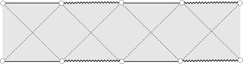
Figure 3: Penrose diagram for the subextremal Schwarzschild-de Sitter spacetime. The excluded points $\mathcal{Q}$, $\mathcal{Q^{\prime}}$ represent asymptotic regions where the Cosmological horizon appear to meet $\mathscr{I}$. As discussed in Section 3.1 this region of the spacetime does not belong to $\mathscr{I}$.

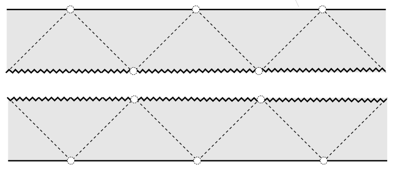
Figure 4: Penrose diagrams for the extremal Schwarzschild-de Sitter spacetime. Case (a) corresponds to a white hole which evolves towards a de Sitter final state while case (b) is a model of a black hole with a future singularity. The continuous black line denotes the conformal boundary; the serrated line denotes the location of the singularity; the dashed line shows the location of the Killing horizons $\mathcal{H}$ at $r=3m$ . The excluded points $\mathcal{Q}$, $\mathcal{Q^{\prime}}$ and $\mathcal{P}$ represent asymptotic regions of the spacetime that do not belong to $\mathscr{I}$ or the singularity $r=0$.

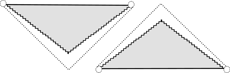
Figure 5: Penrose diagram for the hyperextremal Schwarzschild-de Sitter spacetime. The singularity is of spacelike nature. Dotted lines at 45 ^∘ and 135 ^∘ have been included for visualisation. Case (a) corresponds to a white hole which evolves to a final de-Sitter state. Case (b) corresponds to a black hole with a future spacelike singularity.

3.2 The $\mathbb{S}^{3}\backslash\{\mathcal{Q},\mathcal{Q^{\prime}}\}$-representation

The basic conformal structure of the subextremal and extremal Schwarzschild-de Sitter spacetimes has already been discussed in [2, 7] and [47] respectively. Coordinate and Penrose diagrams have been also provided in [32] for the subextremal, extremal and hyperextremal cases. In this section we present a concise discussion, adapted to our conventions, of the conformal structure of the Schwarzschild-de Sitter spacetime in the subextremal, extremal and hyperextremal cases. We start our discussion showing that irrespective of the relation of $m$ and $\lambda$ the induced metric at the conformal boundary for the Schwarzschild de Sitter spacetime can be identified with the standard metric on $\mathbb{S}^{3}$. As discussed in more detail in Section 3.3.1, this construction depends on the particular conformal representation being considered. In the subextremal case one cannot obtain simultaneously an analytic extension regular near both $r_{b}$ and $r_{c}$—see [2]. Since we are interested only in the asymptotic region, in this section we will consider the region $r>r_{c}$. For the extremal and hyperextremal cases such considerations are not necessary.

In the following we introduce the null coordinates

$$u\equiv\sqrt{|\lambda|}(t-\mathfrak{r}),\qquad v\equiv\sqrt{|\lambda|}(t+\mathfrak{r}),$$

where $\mathfrak{r}$ is a tortoise coordinate given by

$$\mathfrak{r}\equiv\int\frac{1}{F(r)}dr.$$ (48)

This integral can be computed explicitly —see [2, 7]. The particular form of $\mathfrak{r}$ depends on the relation between $\lambda$ and $m$. As discussed in [7, 47] the integration constant can always be chosen so that $\mathfrak{r}\rightarrow 0$ as $r\rightarrow\infty$. Defining $\tan U\equiv u,\tan V\equiv v$, with $U,V\in[-\tfrac{\pi}{2},\tfrac{\pi}{2}]$ one gets the line element

$$\tilde{{\bm{g}}}_{SdS}=\frac{1}{2}\frac{F(r)}{|\lambda|}\sec^{2}{U}\sec^{2}{V}\left(\mathbf{d}U\otimes\mathbf{d}V+\mathbf{d}V\otimes\mathbf{d}U\right)-r^{2}{\bm{\sigma}}.$$ (49)

As discussed in [7, 2], one can construct Kruskal type coordinates covering the black hole horizon by choosing appropriately the integration constant in equation (48). Analogously, choosing a different integration constant, one can construct Kruskal type coordinates covering the cosmological horizon. Nevertheless in the subextremal case, as emphasised in [2], it is not possible to construct Kruskal type coordinates covering simultaneously both horizons. To construct the Penrose diagram for this spacetime, one considers as building blocks the Penrose diagrams for the regions $0\leq r\leq r_{b}$, $r_{b}\leq r\leq r_{c}$ and $r_{c}\leq r<\infty$ which are then glued together using the corresponding Kruskal type coordinates to cross each horizon —see [2, 32] for a detailed discussion on the construction the Penrose diagram and Kruskal type coordinates in the Schwarzschild-de Sitter spacetime. Consistent with the above discussion and given that we are only interested in the asymptotic region, we restrict our attention, in the subextremal case, to $r>r_{c}$. In the extremal case one has, however, that $r_{b}=r_{c}=3m$ and one can verify that

$$\lim_{r\to 3m}\frac{\cos U}{r-3m}=\lim_{r\to 3m}\frac{\cos V}{r-3m}=C,$$

where $C\neq 0$ is a constant depending on $m$ and the integration constant chosen in the definition of $\mathfrak{r}$. Consequently, in the extremal case, the metric (49) is well defined for the whole range of the coordinate $r$: $0<r<\infty$ —see [47]. Introducing the coordinates $(\bar{U},\bar{V})$ defined via

$$\tan U\equiv\ln\tan\bigg{(}\frac{\pi}{4}+\frac{\bar{U}}{2}\bigg{)},\qquad\tan V\equiv\ln\tan\bigg{(}\frac{\pi}{4}+\frac{\bar{V}}{2}\bigg{)}$$

one obtains

$$\tilde{{\bm{g}}}_{SdS}=\frac{1}{2}\frac{F(r)}{|\lambda|}\sec{\bar{U}}\sec{\bar{V}}\left(\mathbf{d}\bar{U}\otimes\mathbf{d}\bar{V}+\mathbf{d}\bar{V}\otimes\mathbf{d}\bar{U}\right)-r^{2}{\bm{\sigma}}.$$

Recalling that in the subextremal case $F(r)\leq 0$ for $r\geq r_{c}$ while for the extremal and hyperextremal cases $F(r)\leq 0$ for $0<r<\infty$, one identifies the conformal factor

$$\Xi^{2}=\frac{|\lambda|}{|F(r)|}\cos\bar{U}\cos\bar{V}.$$

Therefore, we can identify the conformal metric ${\bm{g}}_{SdS}=\Xi^{2}\tilde{{\bm{g}}}_{SdS}$ with

$${\bm{g}}_{SdS}=-\frac{1}{2}\left(\mathbf{d}\bar{U}\otimes\mathbf{d}\bar{V}+\mathbf{d}\bar{V}\otimes\mathbf{d}\bar{U}\right)-\frac{|\lambda|r^{2}}{|F(r)|}\cos\bar{U}\cos\bar{V}\bm{\sigma}.$$ (50)

Introducing the coordinates

$$T\equiv\bar{U}+\bar{V},\qquad\Psi\equiv\bar{V}-\bar{U},$$

one gets

$${\bm{g}}_{SdS}=\frac{1}{4}\left(\mathbf{d}\Psi\otimes\mathbf{d}\Psi-\mathbf{d}T\otimes\mathbf{d}T\right)-\frac{|\lambda|r^{2}}{|F(r)|}\cos\frac{1}{2}\left(T+\Psi\right)\cos\frac{1}{2}\left(T-\Psi\right)\bm{\sigma}.$$

The analysis in [2] shows that the conformal factor $\Xi$ tends to zero as $r\rightarrow\infty$. Hence, to identify the induced metric at $\mathscr{I}$ it is sufficient to analyse such limit. Noticing that

$$\mathfrak{r}=\frac{1}{2\sqrt{|\lambda|}}(v-u)=\frac{1}{2\sqrt{|\lambda|}}\ln\left(\frac{\tan(\pi/4+\bar{V})}{\tan(\pi/4+\bar{U})}\right)$$

and recalling that

$$\lim_{r\rightarrow\infty}\mathfrak{r}=0,$$

one concludes that $r\rightarrow\infty$ implies $\Psi=0$ as long as $\bar{U}\neq\pm\tfrac{1}{2}\pi$ and $\bar{V}\neq\pm\tfrac{1}{2}\pi$. Using equation (43) one can verify that

$$\lim_{r\rightarrow\infty}\frac{|\lambda|r^{2}}{|F(r)|}=1.$$

Consequently, the induced metric on $\mathscr{I}$ is given by

$${\bm{h}}=-\frac{1}{4}\mathbf{d}T\otimes\mathbf{d}T-\cos^{2}\frac{T}{2}\bm{\sigma}$$

which can be written in a more recognisable form introducing $\xi\equiv\tfrac{1}{2}(T+\pi)$ so that

$${\bm{\hbar}}=-\mathbf{d}\xi\otimes\mathbf{d}\xi-\sin^{2}\xi\bm{\sigma}.$$ (51)

The metric ${\bm{\hbar}}$ is the standard metric on $\mathbb{S}^{3}$. Observe that the excluded points in the discussion of this section $(\bar{U},\bar{V})=(\pm\tfrac{1}{2}\pi,\pm\tfrac{1}{2}\pi)$ correspond to $\xi=0$ and $\xi=\pi$ —the North and South pole of $\mathbb{S}^{3}$. The Penrose diagram of the subextremal, extremal and hyperextremal Schwarzschild-de Sitter spacetime is given in Figure 4 (a). The conformal boundary $\mathscr{I}$ of the (subextremal, extremal and hyperextremal) Schwarzschild-de Sitter spacetime, defined by the condition $\Xi=0$, is spacelike consistent with the fact that the Cosmological constant of the spacetime is de Sitter-like —see e.g. [46, 51]. Moreover, the singularity at $r=0$ is of a spacelike nature —see [32, 47]. As pointed out in [2, 33], the Schwarzschild-de Sitter spacetime can be interpreted as the model of a white hole singularity towards a final de Sitter state. Alternatively, making use of a reflection

$$u\mapsto-u,\qquad v\mapsto-v,$$

one obtains a model of a black hole with a future singularity —see Figures 3, 4 and 5.

In what follows, we adopt the white hole point of view for the extremal and hyperextremal cases so that $\mathscr{I}$ corresponds to future conformal infinity and we will consider a backward asymptotic initial value problem. Consistent with this point of view, for the subextremal case we consider asymptotic initial data on $\mathscr{I}^{+}$ and study the development of such data towards the curvature singularity located at $r=0$ —see Figure 1.

3.3 The $\mathbb{R}\times\mathbb{S}^{2}$-representation

In Section 3.2 we have shown that there exist a conformal representation in which the induced metric on the conformal boundary corresponds to the standard metric on $\mathbb{S}^{3}$. A quick inspection shows that the metric (51) is conformally flat. In this section we put this observation in a wider perspective and show that the induced metric on $\mathscr{I}$ of a spherically symmetric spacetime with spacelike $\mathscr{I}$ is necessarily conformally flat. In addition, a conformal representation in which the induced metric at the conformal boundary corresponds to the standard metric on $\mathbb{R}\times\mathbb{S}^{2}$ is discussed. This conformal representation will be of particular importance in the subsequent analysis.

3.3.1 The conformal boundary of spherically symmetric and asymptotically de Sitter spacetimes

Following an argument similar to the one given in [43] we have the following construction for a spherically symmetric spacetime with spacelike conformal boundary: if a spacetime $(\tilde{\mathcal{M}},\tilde{{\bm{g}}})$ is spherically symmetric then the metric $\tilde{{\bm{g}}}$ can be written in a warped product form

$$\tilde{{\bm{g}}}=\tilde{{\bm{\gamma}}}-\tilde{\rho}^{2}{\bm{\sigma}},$$ (52)

where $\tilde{{\bm{\gamma}}}$ is the 2-metric on the quotient manifold $\tilde{\mathcal{Q}}\equiv\mathcal{\tilde{M}}/SO(3)$, ${\bm{\sigma}}$ is the standard metric of $\mathbb{S}^{2}$ and $\tilde{\rho}:\tilde{\mathcal{Q}}\rightarrow\mathbb{R}$. If ${\bm{g}}$ and $\tilde{{\bm{g}}}$ are conformally related, ${\bm{g}}=\Theta^{2}\tilde{{\bm{g}}}$, then the spherical symmetry condition for ${\bm{g}}$ is translated into the requirement that ${\bm{g}}$ can be written in the form

$${\bm{g}}={\bm{\gamma}}-\rho^{2}{\bm{\sigma}},$$

where ${\bm{\gamma}}\equiv\Theta\tilde{{\bm{\gamma}}}$ and $\rho\equiv\Theta\tilde{\rho}$, where $\Theta$ does not depend on the coordinates on $\mathbb{S}^{2}$. Near $\mathscr{I}$ let us introduce local coordinates $(\Theta,\psi)$ on the quotient manifold $\mathcal{Q}\equiv\mathcal{M}/SO(3)$ so that $\Theta=0$ denotes the locus of $\mathscr{I}$. Since the conformal boundary is spacelike we have that ${\bm{g}}(\mathbf{d}\Theta,\mathbf{d}\Theta)>0$. Therefore, the metric induced on $\mathscr{I}$ by ${\bm{g}}$ has the form

$${\bm{h}}=-A(\psi)\mathbf{d}\psi\otimes\mathbf{d}\psi-\rho^{2}(\psi){\bm{\sigma}},$$

where $A(\psi)$ is a positive function. Redefining the coordinate $\psi$ we can rewrite ${\bm{h}}$ as

$${\bm{h}}=-\rho^{2}(\psi)(\mathbf{d}\psi\otimes\mathbf{d}\psi+{\bm{\sigma}}).$$

It can be readily verified —say, by calculating the Cotton tensor of ${\bm{h}}$— that the metric ${\bm{h}}$ is conformally flat. In Section 3.4 it will be shown that, in view of the conformal freedom of the setting, a convenient choice is to consider a conformal representation in which the the 3-metric on $\mathscr{I}$ is given by

$${\bm{h}}=-\mathbf{d}\psi\otimes\mathbf{d}\psi-\bm{\sigma}.$$ (53)

This metric is the standard metric of the cylinder $\mathbb{R}\times\mathbb{S}^{2}$ with $\psi\in(-\infty,\infty)$. It can be verified that this conformal representation is related to the one discussed in Section 3.2 via ${\bm{h}}=\omega^{2}\bm{\hbar}$, where the conformal factor $\omega$ and the relation between the coordinates are given by

$$\psi(\xi)=\psi_{\star}-\ln|\csc\xi+\cot\xi|,\qquad\omega(\xi)=\csc(\xi).$$ (54)

Equivalently, one has that

$$\xi(\psi)=\arccos\left(\frac{e^{2(\psi_{\star}-\psi)}-1}{e^{2(\psi_{\star}-\psi)}+1}\right),\qquad\omega(\psi)=\frac{e^{\psi}}{2e^{\psi_{\star}}}(e^{2\psi_{\star}}+e^{2\psi}),$$

where $\psi_{\star}$ is a constant of integration. We can directly observe that in this representation $\xi=0$ and $\xi=\pi$ correspond to $\psi=-\infty$ and $\psi=\infty$, respectively.

3.3.2 The extrinsic curvature of the conformal boundary in the $\mathbb{R}\times\mathbb{S}^{2}$ representation

A particularly simple conformal representation for the Schwarzschild-de Sitter spacetime can be obtained using the discussion of Section 3.3.1. Accordingly, take the metric of the Schwarzschild-de Sitter spacetime as written in equation (42) with $F(r)$ as given by the relation (43) and consider the conformal factor $\wideparen{\Xi}\equiv 1/r$. Introducing the coordinates $\varrho\equiv{1}/{r}$ and $\zeta\equiv\sqrt{|\lambda|/3}t$, the conformal metric

$$\wideparen{{\bm{g}}}\equiv\wideparen{\Xi}^{2}{}\tilde{{\bm{g}}}_{eSdS}$$

is given by

$$\wideparen{{\bm{g}}}=\frac{3}{|\lambda|}\Big{(}\varrho^{2}-2m\varrho^{3}-\frac{1}{3}|\lambda|\Big{)}\mathbf{d}\zeta\otimes\mathbf{d}\zeta-\Big{(}\varrho^{2}-2m\varrho^{3}-\frac{1}{3}|\lambda|\Big{)}^{-1}\mathbf{d}\varrho\otimes\mathbf{d}\varrho-{\bm{\sigma}}.$$

The induced metric on the hypersurface described by the condition $\wideparen{\Xi}=0$ is given by

$$\wideparen{{\bm{h}}}=-\mathbf{d}\zeta\otimes\mathbf{d}\zeta-{\bm{\sigma}}.$$

It can be verified that $\wideparen{{\bm{g}}}$ satisfies a conformal gauge for which the conformal boundary has vanishing extrinsic curvature. To see this, consider a $\wideparen{{\bm{g}}}$-orthonormal coframe $\{{\bm{\omega}}^{\bm{a}}\}$ with

$$\bm{\omega}^{0}=\sqrt{\frac{3}{|\lambda|}}\left(\varrho^{2}-2m\varrho^{3}-\frac{1}{3}|\lambda|\right)^{1/2}\mathbf{d}\zeta,\qquad\bm{\omega}^{3}=\left(\varrho^{2}-2m\varrho^{3}-\frac{1}{3}|\lambda|\right)^{-1/2}\mathbf{d}\varrho,$$

and $\{{\bm{\omega}}^{1},\,{\bm{\omega}}^{2}\}$ a ${\bm{\sigma}}$-orthonormal coframe. Denote by $\{{\bm{e}}_{\bm{a}}\}$ the corresponding dual frame. Using this frame we can directly compute the Friedrich scalar $\wideparen{s}\equiv\tfrac{1}{4}\wideparen{\nabla}^{{\bm{c}}}\wideparen{\nabla}_{{\bm{c}}}\wideparen{\Xi}+\tfrac{1}{24}\wideparen{R}\hskip 2.84526pt\wideparen{\Xi}$ —see Appendix D. The computation of the Ricci scalar yields

$$\wideparen{R}=-12m\varrho.$$ (55)

A direct calculation using

$$\wideparen{\nabla}_{\mu}\wideparen{\nabla}^{\mu}\Xi=\frac{1}{\sqrt{-\det\wideparen{{\bm{g}}}}}\partial_{\mu}(\sqrt{-\det\wideparen{{\bm{g}}}}\hskip 2.84526pt\wideparen{g}^{\mu\nu}\partial_{\nu}\Xi)$$

shows that $\wideparen{\nabla}_{a}\wideparen{\nabla}^{a}\Xi=6m\varrho^{2}-2\varrho$. Consequently, the scalar $\wideparen{s}$ vanishes at the hypersurface defined by $\wideparen{\Xi}=\varrho=0$. Contrasting this result with the solution to the conformal constraints given in equations (34a)-(34b) we conclude that in this representation the hypersurface described by $\wideparen{\Xi}=0$ has vanishing extrinsic curvature as claimed.

Remark 4.

Notice that, in this representation the curvature singularity, located $r=0$, corresponds to $\varrho=\infty$. Consequently, $\mathscr{I}$ is at an infinite distance from the conformal boundary.

Observe that, the components of the Weyl tensor with respect to the orthonormal frame $\{{\bm{e}}_{\bm{a}}\}$ as described above are given by

$$C_{1212}=-2m\varrho,\hskip 5.69046ptC_{1313}=m\varrho,\hskip 5.69046ptC_{1010}=-m\varrho,\hskip 5.69046ptC_{2323}=m\varrho,\hskip 5.69046ptC_{2020}=-m\varrho,\hskip 5.69046ptC_{3030}=2m\varrho.$$

This information will be required in the discussion of the initial data for the rescaled Weyl tensor —see Section 3.4.2. Using now that $d_{{\bm{a}}{\bm{b}}{\bm{c}}{\bm{d}}}=\Xi^{-1}C_{{\bm{a}}{\bm{b}}{\bm{c}}{\bm{d}}}$ with $\wideparen{\Xi}=\xi$ and exploiting the fact that the computations have been carried out in an orthonormal frame so that $C^{{\bm{a}}}{}_{{\bm{b}}{\bm{c}}{\bm{d}}}=\eta^{{\bm{a}}{\bm{f}}}C_{{\bm{f}}{\bm{b}}{\bm{c}}{\bm{d}}}$, we get

$$d_{1212}=-2m,\hskip 14.22636ptd_{1313}=m,\hskip 14.22636ptd_{1010}=-m,\hskip 14.22636ptd_{2323}=m,\hskip 14.22636ptd_{2020}=-m,\hskip 14.22636ptd_{3030}=2m.$$

Finally, considering $d_{ij}\equiv d_{i0j0}$ we have

$$d_{11}=-m,\hskip 8.5359ptd_{22}=-m,\hskip 8.5359ptd_{33}=2m.$$ (56)

3.4 Identifying asymptotic regular data

As discussed in Section 3.1, there is a conformal representation in which the induced metric on the conformal boundary of the Schwarzschild-de Sitter is the standard metric ${\bm{\hbar}}$ on $\mathbb{S}^{3}$. Nevertheless, the asymptotic points $\mathcal{Q}$ and $\mathcal{Q^{\prime}}$, as depicted in the Penrose diagram of Figure 4, are associated to the behaviour of those timelike geodesics which never cross the horizon —see Appendix A. Despite that, from the point of view of the intrinsic geometry of $\mathscr{I}$ these asymptotic regions —corresponding to the North and South poles of $\mathbb{S}^{3}$— are regular, from a spacetime point of view they are not. This issue will be further discussed Section 3.4.2 where it will be shown that the initial data for the electric part of rescaled Weyl tensor is singular at $\mathcal{Q}$ and $\mathcal{Q^{\prime}}$. Fortunately, as exposed in Section 2.4.2 one can exploit the inherent conformal freedom of the setting to select any representative of the conformal class $[{\bm{\hbar}}]$ to construct a solution to the conformal constraint equations. Taking into account the previous remarks it will be convenient to choose the conformal representation discussed in Section 3.3, ${\bm{h}}=\omega^{2}{\bm{\hbar}}$ with $\omega$ and ${\bm{h}}$ given in equations (53) and (54), in which the points $\mathcal{Q}$ and $\mathcal{Q^{\prime}}$ are at infinity respect to the metric ${\bm{h}}$.

3.4.1 A frame for the induced metric at $\mathscr{I}$

Consistent with the discussion of the last section, on $\mathscr{I}$ one considers an adapted frame $\{{\bm{l}},\,{\bm{m}},\bar{{\bm{m}}}\}$ such that the metric (53) can be written in the form

$${\bm{h}}=-({\bm{l}}\otimes{\bm{l}}+{\bm{\sigma}})$$

where

$${\bm{l}}=\mathbf{d}\psi,\qquad\bm{\sigma}=\frac{1}{2}({\bm{m}}\otimes\bar{{\bm{m}}}+\bar{{\bm{m}}}\otimes{\bm{m}}).$$

In terms of abstract index notation we have

$$h_{ij}=-l_{i}l_{j}-2m_{(i}\bar{m}_{j)}.$$ (57)

The frame $\{{\bm{l}},\,{\bm{m}},\bar{{\bm{m}}}\}$ satisfies the pairings

$$l_{j}l^{j}=-1,\qquad m_{j}\bar{m}^{j}=-1,\qquad l_{j}m^{j}=l_{j}\bar{m}^{j}=m_{j}m^{j}=\bar{m}_{j}\bar{m}^{j}=0.$$ (58)

3.4.2 Initial data for the rescaled Weyl tensor

The procedure for the construction of a solution to the conformal constraints at the conformal boundary requires, in particular, a solution to the divergence equation (35) for the electric part of the rescaled Weyl tensor. The requirement of spherical symmetry of the spacetime can be succinctly incorporated using the results in [44]. If the unphysical spacetime $(\mathcal{M},{\bm{g}})$ possesses a Killing vector ${\bm{X}}$ then the initial data encoded in the symmetric tracefree tensor $d_{ij}$ must satisfy the condition

$$\pounds_{{\bm{X}}}d_{ij}=0,$$ (59)

where $\pounds_{{\bm{X}}}$ denotes the Lie derivative in the direction of ${\bm{X}}$ on the initial hypersurface. The only symmetric tracefree tensor $d_{{\bm{i}}{\bm{j}}}$ compatible with the above requirement is given by

$$d_{ij}=\frac{1}{2}\varsigma(3l_{i}l_{j}+h_{ij}).$$ (60)

where $\varsigma=d_{ij}l^{i}l^{j}$.

TT-tensors on $\mathbb{R}^{3}$. The general form of symmetric, tracefree and divergence-free tensors (i.e. TT-tensors) in a conformally flat setting are well-known —see e.g. [3, 9]. For convenience of the reader, in this short paragraph, we adapt the conventions and discussion given in the latter references to the present setting. The general the solutions to the equation

$$\grave{D}^{{\bm{i}}}\grave{d}_{{\bm{i}}{\bm{j}}}=0,$$ (61)

where $\grave{{\bm{h}}}\equiv-{\bm{\delta}}$ is the flat metric has been given in [9]. One can introduce Cartesian coordinates $(x^{{\bm{\alpha}}})$ with the origin of $\mathbb{R}^{3}$ located at a fiduciary position $\mathcal{O}$. Additionally, we introduce polar coordinates defined via $\rho=\delta_{{\bm{\alpha}}{\bm{\beta}}}x^{{\bm{\alpha}}}x^{{\bm{\beta}}}$. The flat metric in these coordinates reads

$$\grave{{\bm{h}}}=-\mathbf{d}\rho\otimes\mathbf{d}\rho-\rho^{2}{\bm{\sigma}}.$$ (62)

Using this notation and taking into account the requirement of spherical symmetry encoded in equation (59) the flat space counterpart of the required solution is

$$\grave{{\bm{d}}}=\frac{A_{\star}}{\rho^{3}}\left(3\mathbf{d}\rho\otimes\mathbf{d}\rho+\grave{{\bm{h}}}\right),$$

where $A_{\star}$ is a constant. In order to obtain an analogous solution in conformally related 3-manifolds one can exploit the conformal properties of equation (61) using the following:

Lemma 6.

Let $\bar{d}_{ij}$ be a tracefree symmetric solution to $\bar{D}^{i}\bar{d}_{ij}=0$ where $\bar{D}$ is the Levi-Civita connection of $\bar{{\bm{h}}}$. Let ${\bm{h}}=\omega^{2}\bar{{\bm{h}}}$, then $d_{ij}=\omega^{-1}\bar{d}_{ij}$ is a symmetric tracefree solution to $D^{i}d_{ij}=0$ where $D$ is the Levi-Civita connection of ${\bm{h}}$.

This lemma can be found in [9]. Here we have adapted the statement to agree with the conventions of this article.

TT-tensors on $\mathbb{S}^{3}$ and $\mathbb{R}\times\mathbb{S}^{2}$. One can exploit Lemma 6 to derive spherically symmetric solutions of the divergence equation (61) in conformally flat 3-manifolds. In particular, the metrics ${\bm{\hbar}}$ and $\grave{{\bm{h}}}$ as given in equations (51) and (62) are related via

$${\bm{\hbar}}=\omega^{2}\grave{{\bm{h}}},$$

where

$$\rho(\xi)=\cot(\xi/2),\qquad\omega(\xi)=2\sin^{2}(\xi/2),$$ (63)

The coordinate transformation $\rho(\xi)$ corresponds to the stereographic projection in which the origin $\mathcal{O}$ of $\mathbb{R}^{3}$ is mapped to the South pole on $\mathbb{S}^{3}$. Alternatively, one can also derive

$$\rho(\xi)=\tan(\xi/2),\qquad\omega(\xi)=2\cos^{2}(\xi/2),$$ (64)

corresponding to the stereographic projection in which the origin of $\mathbb{R}^{3}$ is mapped to the North pole of $\mathbb{S}^{3}$. Using Lemma 6 with equations (63) or (64) one obtains

$$\bm{\mathchar 22\relax\mkern-13.0mud}=\frac{A_{\star}}{2\sqrt{1-\omega^{2}(\xi)}}\left(3\mathbf{d}\xi\otimes\mathbf{d}\xi+{\bm{\hbar}}\right).$$ (65)

Observe that $\mathchar 22\relax\mkern-13.0mud_{{\bm{i}}{\bm{j}}}$ is singular when $\omega(\xi)=1$ which corresponds to $\xi=0$ and $\xi=\pi$ according to equations (63) and (64), respectively. Therefore, in this conformal representation the electric part of the rescaled Weyl tensor is singular at the North and South poles of $\mathbb{S}^{3}$. Proceeding in a analogous way as in the previous paragraphs one can observe that the metrics ${\bm{h}}$ and $\grave{{\bm{h}}}$ given in equations (53) and (62) are related via

$${\bm{h}}=\omega^{2}\grave{{\bm{h}}}$$

where

$$\rho(\psi)=e^{\psi},\qquad\omega(\psi)=e^{-\psi}.$$

A straightforward computation using Lemma 6 renders

$$\bm{d}=A_{\star}\left(3\mathbf{d}\psi\otimes\mathbf{d}\psi+{\bm{h}}\right).$$ (66)

Moreover, since $D^{i}d_{ij}=3A_{\star}D^{i}(l_{i}l_{j})$, it follows that verifying that $d_{ij}$ satisfies the condition (59) reduces to the computation of $\omega_{i}\equiv\pounds_{{\bm{X}}}l_{i}$ and showing that the components of $\omega_{i}$ along any leg of the frame vanishes —that is

$$l^{i}\omega_{i}=0,\qquad m^{i}\omega_{i}=0,\qquad\bar{m}^{i}\omega_{i}=0.$$

The latter can easily be done using the Killing equation $\pounds_{{\bm{X}}}h_{ij}=2D_{(i}X_{j)}=0$ along with equations (57) and (58). Finally, comparing expression (66) with equation (56) we can recognise that $A_{\star}=m$. Observe that this identification is irrespective of the extrinsic curvature of $\mathscr{I}$.

3.5 Asymptotic initial data for the Schwarzschild-de Sitter spacetime

In the last section it was shown that the $\mathbb{R}\times\mathbb{S}^{2}$-conformal representation leads to regular asymptotic data for the rescaled Weyl tensor. In this section we complete the discussion the asymptotic initial data for the Schwarzschild-de Sitter spacetime in this conformal representation. To do so, we make use of the procedure to solve the conformal constraints at the conformal boundary as discussed in Section 2.3.4 and the specific properties of the Schwarzschild-de Sitter spacetime.

3.5.1 Initial data for the Schouten tensor

Computing the Schouten tensor ${\bm{S}}{{\bm{c}}}{\bm{h}}[{\bm{h}}]$ of ${\bm{h}}$ we get that

$${\bm{S}}{{\bm{c}}}{\bm{h}}[{\bm{h}}]=-\frac{1}{2}\mathbf{d}\psi\otimes\mathbf{d}\psi+\frac{1}{2}{\bm{\sigma}}.$$

Equivalently, in abstract index notation one writes

$$l_{ij}=-l_{i}l_{j}-\frac{1}{2}h_{ij}.$$

Thus, recalling the solution to the conformal constraints given in equation (34b) we get,

$$L_{ij}=-l_{i}l_{j}-\frac{1}{2}(1-\kappa^{2})h_{ij}.$$

3.5.2 Initial data for the connection coefficients

In order to compute the connection coefficients associated with the coframe $\{{\bm{\omega}}_{\bm{i}}\}$ recall that ${\bm{\omega}}^{3}=\mathbf{d}\psi$ and $\{{\bm{\omega}}^{1},{\bm{\omega}}^{2}\}$ are ${\bm{\sigma}}$-orthonormal. Equivalently, one has that $\{{\bm{e}}_{\bm{i}}\}=\{{\bm{\partial}}_{\psi},{\bm{e}}_{\bm{1}},{\bm{e}}_{\bm{2}}\}$ with

$${\bm{e}}_{\bm{1}}=\frac{1}{\sqrt{2}}({\bm{m}}+\bar{{\bm{m}}}),\hskip 28.45274pt{\bm{e}}_{\bm{2}}=\frac{\mbox{i}}{\sqrt{2}}({\bm{m}}-\bar{{\bm{m}}}),$$

where ${\bm{\sigma}}={\bm{m}}\otimes\bar{{\bm{m}}}+\bar{{\bm{m}}}\otimes{\bm{m}}$, so that

$${\bm{h}}=-\bm{\omega}^{1}\otimes\bm{\omega}^{1}-\bm{\omega}^{2}\otimes\bm{\omega}^{2}-\bm{\omega}^{3}\otimes\bm{\omega}^{3}.$$

The connection coefficients can be obtained using the first structure equation (116a) given in Appendix C.1. Proceeding in this manner, by a straightforward computation, one can show that the only non-zero connection coefficient is $\gamma_{2}{}^{2}{}_{1}$. In terms of the Ricci-rotation coefficients, the latter corresponds to $2\sqrt{2}\operatorname{Re}(\alpha_{\star})$ where $\alpha_{\star}=-\frac{1}{2}\bar{m}^{a}\bar{\delta}m_{a}$ in the standard NP notation —see [51]. Therefore, the only no-trivial initial data for the connection coefficients is

$$\gamma_{2}{}^{2}{}_{1}=\sqrt{2}(\alpha_{\star}+\bar{\alpha}_{\star}).$$

Remark 4. The frame over the cylinder $\mathbb{R}\times\mathbb{S}^{2}$ introduced in this section is not a global one. Nevertheless, it is possible to construct an atlas covering $\mathbb{R}\times\mathbb{S}^{2}$ such that one each of the charts one has a well defined frame of the required form.

3.5.3 Spinorial initial data

In this section we discuss the spinorial counterpart of the asymptotic initial data computed in the previous sections.

3.5.4 Spin connection coefficients

The spinorial counterpart of the asymptotic initial data constructed in the previous sections is readily obtained by suitable contraction with the spatial Infeld-van der Waerden symbols —see Appendix C.3. Following the discussion of Section 3.5.2, let ${\bm{\omega}}^{3}=\mathbf{d}\psi$ and let $\{{\bm{\omega}}^{1},{\bm{\omega}}^{2}\}$ denote an ${\bm{\sigma}}$-orthonormal coframe. Using equations (123b) of Appendix C.3 we have that the spinorial coframe is given by

$${\bm{\omega}}^{{\bm{A}}{\bm{B}}}=\sigma_{{\bm{i}}}{}^{{\bm{A}}{\bm{B}}}{\bm{\omega}}^{{\bm{i}}}=(y^{{\bm{A}}{\bm{B}}}+z^{{\bm{A}}{\bm{B}}}){\bm{\omega}}^{1}+\mbox{i}(y^{{\bm{A}}{\bm{B}}}-z^{{\bm{A}}{\bm{B}}}){\bm{\omega}}^{2}-x^{{\bm{A}}{\bm{B}}}{\bm{\omega}}^{3}.$$ (67)

Alternatively, one has that the spinorial frame is given by

$${\bm{e}}_{{\bm{A}}{\bm{B}}}=x_{{\bm{A}}{\bm{B}}}{\bm{e}}_{x}{}^{3}{\bm{\partial}}_{\psi}+\sqrt{2}y_{{\bm{A}}{\bm{B}}}e_{y}{}^{+}\bar{{\bm{m}}}^{\flat}+\sqrt{2}z_{{\bm{A}}{\bm{B}}}e_{z}{}^{-}{\bm{m}}^{\flat}$$

where ${\bm{e}}_{x}{}^{3}$, ${\bm{e}}_{y}{}^{+}$, ${\bm{e}}_{z}{}^{-}$ denote the only non-vanishing frame coefficients. Equation (67) allow us to compute the reduced connection coefficients $\gamma_{{\bm{A}}}{}^{{\bm{B}}}{}_{{\bm{C}}{\bm{D}}}$ using the first Cartan structure equation (122a) in Appendix C.3. Alternatively, one can use the results of Section 3.5.2 and the spatial Infeld-van der Waerden symbols to compute

$$\gamma_{{\bm{A}}{\bm{B}}}{}^{{\bm{C}}{\bm{D}}}{}_{{\bm{E}}{\bm{F}}}\equiv\gamma_{{\bm{i}}}{}^{{\bm{j}}}{}_{{\bm{k}}}\sigma_{{\bm{A}}{\bm{B}}}{}^{{\bm{i}}}\sigma^{{\bm{C}}{\bm{D}}}{}_{{\bm{j}}}\sigma_{{\bm{E}}{\bm{F}}}{}^{{\bm{k}}},$$

where

$$\gamma_{{\bm{i}}}{}^{{\bm{j}}}{}_{{\bm{k}}}=\delta_{{\bm{i}}}{}^{2}\delta_{1}{}^{{\bm{j}}}\delta_{{\bm{k}}}{}^{2}\gamma_{2}{}^{1}{}_{2}+\delta_{{\bm{i}}}{}^{2}\delta_{2}{}^{{\bm{j}}}\delta_{{\bm{k}}}{}^{1}\gamma_{2}{}^{2}{}_{1},$$

with

$$\gamma_{2}{}^{1}{}_{2}=-\sqrt{2}(\alpha_{\star}+\bar{\alpha}_{\star}),\qquad\gamma_{2}{}^{2}{}_{1}=\sqrt{2}(\alpha_{\star}+\bar{\alpha}_{\star}).$$

Using the identities (123a)-(123b) in Appendix C.3 one obtains

$$\gamma_{{\bm{A}}{\bm{B}}}{}^{{\bm{C}}{\bm{D}}}{}_{{\bm{E}}{\bm{F}}}=2\sqrt{2}(\alpha_{\star}+\bar{\alpha}_{\star})(y_{{\bm{A}}{\bm{B}}}-z_{{\bm{A}}{\bm{B}}})(y_{{\bm{E}}{\bm{F}}}z^{{\bm{C}}{\bm{D}}}-y^{{\bm{C}}{\bm{D}}}z_{{\bm{E}}{\bm{F}}}).$$

Thus, the reduced connection coefficients are given by

$$\gamma_{{\bm{A}}{\bm{B}}}{}^{{\bm{D}}}{}_{{\bm{F}}}\equiv\frac{1}{2}\gamma_{{\bm{A}}{\bm{B}}}{}^{{\bm{C}}{\bm{D}}}{}_{{\bm{C}}{\bm{D}}}=(\alpha_{\star}+\bar{\alpha}_{\star})x^{{\bm{D}}}{}_{{\bm{F}}}(y_{{\bm{A}}{\bm{B}}}-z_{{\bm{A}}{\bm{B}}}).$$ (68)

By computing the spinor version of the connection form ${\bm{\gamma}}^{{\bm{D}}}{}_{{\bm{F}}}\equiv\gamma_{{\bm{A}}{\bm{B}}}{}^{{\bm{D}}}{}_{{\bm{F}}}{\bm{\omega}}^{{\bm{A}}{\bm{B}}}$ using equations (68) and (67) one can readily verify that the first structure equation is satisfied. Additionally, using the reality conditions,

$$x_{{\bm{A}}{\bm{B}}}{}^{\dagger}=-x_{{\bm{A}}{\bm{B}}},\qquad y_{{\bm{A}}{\bm{B}}}{}^{\dagger}=z_{{\bm{A}}{\bm{B}}},\qquad z_{{\bm{A}}{\bm{B}}}{}^{\dagger}=y_{{\bm{A}}{\bm{B}}}$$

we can verify that $\gamma_{{\bm{A}}{\bm{B}}{\bm{C}}{\bm{D}}}$ is an imaginary spinor —as is to be expected from the space spinor formalism. The field $\gamma_{{\bm{A}}{\bm{B}}{\bm{C}}{\bm{D}}}$ represents the initial data for the field $\xi_{{\bm{A}}{\bm{B}}{\bm{C}}{\bm{D}}}$ —the imaginary part of the reduced connection coefficient $\Gamma_{{\bm{A}}{\bm{B}}{\bm{C}}{\bm{D}}}$. The real part of $\Gamma_{{\bm{A}}{\bm{B}}{\bm{C}}{\bm{D}}}$ corresponds to the Weingarten spinor $\chi_{{\bm{A}}{\bm{B}}{\bm{C}}{\bm{D}}}$ which, in accordance with equation (34a), is given initially by

$$\chi_{{\bm{A}}{\bm{B}}{\bm{C}}{\bm{D}}}=\kappa h_{{\bm{A}}{\bm{B}}{\bm{C}}{\bm{D}}}.$$

Rewriting the reduced connection coefficients (68) in terms of the basic valence-4 spinors introduced in Section 4.1 we get for $\xi_{{\bm{A}}{\bm{B}}{\bm{C}}{\bm{D}}}=\gamma_{{\bm{A}}{\bm{B}}{\bm{C}}{\bm{D}}}$ the explicit expression

$$\xi_{{\bm{A}}{\bm{B}}{\bm{C}}{\bm{D}}}=-(\alpha_{\star}+\bar{\alpha}_{\star})(\epsilon^{1}{}_{{\bm{A}}{\bm{B}}{\bm{C}}{\bm{D}}}+\epsilon^{3}{}_{{\bm{A}}{\bm{B}}{\bm{C}}{\bm{D}}})$$

$$\hskip 85.35826pt+\frac{1}{2\sqrt{2}}(\alpha_{\star}+\bar{\alpha}_{\star})\epsilon_{{\bm{A}}{\bm{C}}}(y_{{\bm{B}}{\bm{D}}}+z_{{\bm{B}}{\bm{D}}})+\frac{1}{2\sqrt{2}}(\alpha_{\star}+\bar{\alpha}_{\star})\epsilon_{{\bm{B}}{\bm{D}}}(y_{{\bm{A}}{\bm{C}}}+z_{{\bm{A}}{\bm{C}}}).$$

3.5.5 Spinorial counterpart of the Schouten tensor

The spinorial counterpart of the Schouten tensor $l_{ij}$ can be directly read from the expressions in Section 3.5.1. Observe that the elementary spinor $x^{{\bm{A}}{\bm{B}}}$ corresponds to the components of $l_{i}$ with respect to the coframe (67) since

$${\bm{\omega}}^{{\bm{A}}{\bm{B}}}x_{{\bm{A}}{\bm{B}}}=-x^{{\bm{A}}{\bm{B}}}x_{{\bm{A}}{\bm{B}}}{\bm{\omega}}^{3}={\bm{\omega}}^{3}=\mathbf{d}\psi={\bm{l}}.$$

Replacing $h_{{\bm{i}}{\bm{j}}}$ by its space spinor counterpart $h_{{\bm{A}}{\bm{B}}{\bm{C}}{\bm{D}}}$ we obtain

$$l_{{\bm{i}}{\bm{j}}}\mapsto l_{{\bm{A}}{\bm{B}}{\bm{C}}{\bm{D}}}=-x_{{\bm{A}}{\bm{B}}}x_{{\bm{C}}{\bm{D}}}-\frac{1}{2}h_{{\bm{A}}{\bm{B}}{\bm{C}}{\bm{D}}}.$$

Equivalently, recalling that the space spinor counterpart of the tracefree part of a tensor $l_{\{{\bm{i}}{\bm{j}}\}}\equiv l_{{\bm{i}}{\bm{j}}}-\tfrac{1}{3}lh_{{\bm{i}}{\bm{j}}}$ corresponds to the totally symmetric spinor $l_{({\bm{A}}{\bm{B}}{\bm{C}}{\bm{D}})}$ it follows then from

$$l_{{\bm{i}}{\bm{j}}}=l_{\{{\bm{i}}{\bm{j}}\}}+\frac{1}{3}lh_{{\bm{i}}{\bm{j}}},$$

that

$$l_{{\bm{A}}{\bm{B}}{\bm{C}}{\bm{D}}}=l_{({\bm{A}}{\bm{B}}{\bm{C}}{\bm{D}})}+\frac{1}{3}lh_{{\bm{A}}{\bm{B}}{\bm{C}}{\bm{D}}}.$$

Thus, using that for the metric (53) one has $r=-2$ and that $l\equiv h^{{\bm{i}}{\bm{j}}}l_{{\bm{i}}{\bm{j}}}=\frac{1}{4}r$, it follows that $l=-\frac{1}{2}$ and $l_{({\bm{A}}{\bm{B}}{\bm{C}}{\bm{D}})}=-x_{({\bm{A}}{\bm{B}}}x_{{\bm{C}}{\bm{D}})}=-2\epsilon^{2}_{{\bm{A}}{\bm{B}}{\bm{C}}{\bm{D}}}$. Therefore, we get

$$l_{{\bm{A}}{\bm{B}}{\bm{C}}{\bm{D}}}=-2\epsilon^{2}{}_{{\bm{A}}{\bm{B}}{\bm{C}}{\bm{D}}}-\frac{1}{6}h_{{\bm{A}}{\bm{B}}{\bm{C}}{\bm{D}}}.$$ (69)

Finally, recalling the expressions for the components of the spacetime Schouten tensor given in (34b) we conclude

$$L_{{\bm{A}}{\bm{B}}{\bm{C}}{\bm{D}}}=-2\epsilon^{2}{}_{{\bm{A}}{\bm{B}}{\bm{C}}{\bm{D}}}-\frac{1}{6}(1-3\kappa^{2})h_{{\bm{A}}{\bm{B}}{\bm{C}}{\bm{D}}}.$$

3.5.6 Initial data for the rescaled Weyl spinor

Following the approach employed in last section, the spinorial counterpart of (66) is given by

$$d_{{\bm{A}}{\bm{B}}{\bm{C}}{\bm{D}}}=A_{\star}(3l_{{\bm{A}}{\bm{B}}}l_{{\bm{C}}{\bm{D}}}+h_{{\bm{A}}{\bm{B}}{\bm{C}}{\bm{D}}}).$$

However, the trace-freeness condition simplifies the last expression since $d^{{\bm{i}}}{}_{{\bm{i}}}=0$ implies that $d_{{\bm{i}}{\bm{j}}}=d_{\{{\bm{i}}{\bm{j}}\}}$. Therefore $d_{{\bm{A}}{\bm{B}}{\bm{C}}{\bm{D}}}=d_{({\bm{A}}{\bm{B}}{\bm{C}}{\bm{D}})}=3A_{\star}l_{({\bm{A}}{\bm{B}}}l_{{\bm{C}}{\bm{D}})}$. As the elementary spinor $x_{{\bm{A}}{\bm{B}}}$ can be associated to the components of ${\bm{l}}$ respect to the co-frame (67) one gets that

$$d_{{\bm{A}}{\bm{B}}{\bm{C}}{\bm{D}}}=3A_{\star}x_{({\bm{A}}{\bm{B}}}x_{{\bm{C}}{\bm{D}})}.$$

This last expression can be equivalently written in terms of the basic valence-4 space spinors of Section 4.1 as

$$\phi_{{\bm{A}}{\bm{B}}{\bm{C}}{\bm{D}}}=6m\epsilon^{2}{}_{{\bm{A}}{\bm{B}}{\bm{C}}{\bm{D}}}.$$

where, in the absence of a magnetic part, we have identified $\phi_{{\bm{A}}{\bm{B}}{\bm{C}}{\bm{D}}}$ initially with $d_{{\bm{A}}{\bm{B}}{\bm{C}}{\bm{D}}}$. Observe that have set $A_{\star}=m$ consistent with the discussion of Section 3.4.2.

4 The solution to the asymptotic initial value problem for the Schwarzschild-de Sitter spacetime and perturbations

As already discussed in the introductory section, recasting explicitly the Schwarzschild-de Sitter spacetime as a solution to the system of conformal evolution equations (29a)-(29i) requires solving, in an explicit manner, the conformal geodesic equations. This, as discussed in Appendix A.2, is not possible in general. Instead, an alternative approach is to study directly the conformal evolution equations (29a)-(29i) making explicit the spherical symmetry of the solution and the asymptotic initial data corresponding to the Schwarzschild-de Sitter spacetime. This approach does not only extract the required information about the reference solution —in the conformal Gaussian gauge— but, in addition, is a model for the general structure of the conformal evolution equations. The relevant analysis is discussed in Sections 4.1 and 4.2. As a complementary analysis, we study the the formation of singularities in the evolution equations. In order to have a more compact discussion leading to the Main Result, the analysis of the formation of singularities is presented in Appendix B. Finally, in Section 4.3, we use the theory of symmetric hyperbolic systems contained in [37] to obtain a existence and stability result for the development of small perturbations to the asymptotic initial data of the Schwarzschild-de Sitter spacetime.

4.1 The spherically symmetric evolution equations

Hitherto, the discussion of the extended conformal Einstein field equations and the conformal constraint equations has been completely general. Since we are interested in analysing the Schwarzschild-de Sitter spacetime as a solution to the conformal field equations one has to incorporate specific properties of this spacetime. The most important assumption for our analysis is that of the spherical symmetry of the spacetime. Under this assumption, a generalisation of Birkhoff’s theorem for vacuum spacetimes with de Sitter-like Cosmological constant shows that the spacetime must be locally isometric to either the Nariai or the Schwarzschild-de Sitter solutions —see [50]. As the Nariai solution is known to not admit a smooth conformal boundary [5, 26], then the formulation of an asymptotic initial value problem readily selects the Schwarzschild-de Sitter spacetime.

To incorporate the assumption of spherical symmetry into the conformal field equations encoded in the spinorial zero-quantities (19a)-(19d) one has to reexpress the requirement of spherical symmetry in terms of the space spinor formalism. In order to ease the presentation we simply introduce a consistent Ansatz for spherical symmetry —a similar approach has been taken in [43]. More precisely, we set

$$\phi_{{\bm{A}}{\bm{B}}{\bm{C}}{\bm{D}}}=\phi_{2}\,\epsilon^{2}{}_{{\bm{A}}{\bm{B}}{\bm{C}}{\bm{D}}},$$ (70a)

$$\Theta_{{\bm{A}}{\bm{B}}}=\sqrt{2}\Theta_{x}{}^{T}\,x_{{\bm{A}}{\bm{B}}},$$ (70b)

$$\Theta_{{\bm{A}}{\bm{B}}{\bm{C}}{\bm{D}}}=\Theta_{2}{}^{S}\,\epsilon^{2}{}_{{\bm{A}}{\bm{B}}{\bm{C}}{\bm{D}}}+\frac{1}{3}\Theta_{h}{}^{S}\,h_{{\bm{A}}{\bm{B}}{\bm{C}}{\bm{D}}},$$ (70c)

$$\xi_{{\bm{A}}{\bm{B}}{\bm{C}}{\bm{D}}}=\xi_{1}\,\epsilon^{1}{}_{{\bm{A}}{\bm{B}}{\bm{C}}{\bm{D}}}+\xi_{2}\,\epsilon^{2}{}_{{\bm{A}}{\bm{B}}{\bm{C}}{\bm{D}}}+\xi_{3}\,\epsilon^{3}{}_{{\bm{A}}{\bm{B}}{\bm{C}}{\bm{D}}}+\frac{1}{3}\xi_{h}\,h_{{\bm{A}}{\bm{B}}{\bm{C}}{\bm{D}}}$$

$$\hskip 56.9055pt+\frac{\xi_{x}}{\sqrt{2}}(x_{{\bm{B}}{\bm{D}}}\epsilon_{{\bm{A}}{\bm{C}}}+x_{{\bm{A}}{\bm{C}}}\epsilon_{{\bm{B}}{\bm{D}}})+\frac{\xi_{y}}{\sqrt{2}}(y_{{\bm{B}}{\bm{D}}}\epsilon_{{\bm{A}}{\bm{C}}}+y_{{\bm{A}}{\bm{C}}}\epsilon_{{\bm{B}}{\bm{D}}})$$

$$\hskip 56.9055pt+\frac{\xi_{z}}{\sqrt{2}}(z_{{\bm{B}}{\bm{D}}}\epsilon_{{\bm{A}}{\bm{C}}}+z_{{\bm{A}}{\bm{C}}}\epsilon_{{\bm{B}}{\bm{D}}}),$$ (70d)

$$\chi_{{\bm{A}}{\bm{B}}{\bm{C}}{\bm{D}}}=\chi_{2}\,\epsilon^{2}_{{\bm{A}}{\bm{B}}{\bm{C}}{\bm{D}}}+\frac{1}{3}\chi_{h}\,h_{{\bm{A}}{\bm{B}}{\bm{C}}{\bm{D}}},$$ (70e)

$$e^{0}{}_{{\bm{A}}{\bm{B}}}=e^{0}_{x}\,x_{{\bm{A}}{\bm{B}}},\qquad e^{3}_{{\bm{A}}{\bm{B}}}=e^{3}_{x}\,x_{{\bm{A}}{\bm{B}}},\qquad e^{+}_{{\bm{A}}{\bm{B}}}=e^{+}_{y}\,y_{{\bm{A}}{\bm{B}}},\qquad e^{-}_{{\bm{A}}{\bm{B}}}=e^{-}_{z}\,z_{{\bm{A}}{\bm{B}}},$$ (70f)

$$f_{{\bm{A}}{\bm{B}}}=f_{x}\,x_{{\bm{A}}{\bm{B}}},$$ (70g)

$$d_{{\bm{A}}{\bm{B}}}=d_{x}\,x_{{\bm{A}}{\bm{B}}}.$$ (70h)

The elementary spinors $x_{{\bm{A}}{\bm{B}}}$, $y_{{\bm{A}}{\bm{B}}}$, $z_{{\bm{A}}{\bm{B}}}$, $\epsilon^{2}_{{\bm{A}}{\bm{B}}{\bm{C}}{\bm{D}}}$ and $h_{{\bm{A}}{\bm{B}}{\bm{C}}{\bm{D}}}$ used in the above Ansatz are defined in Appendix C.2. For further details on the construction of a general spherically symmetric Ansatz see [21, 54]. Alternatively, one can follow a procedure similar to that of Section 3.5.4 —by writing a consistent spherically symmetric Ansatz for the orthonormal frame one can identify the non-vanishing components of the required tensors. The transition to the spinorial version of such Ansatz can be obtained by contracting appropriately with the Infeld-van der Waerden symbols taking into account equations (123a)-(123b), (119a)-(119d) and (120a)-(120c).

The Ansatz for spherical symmetry encoded in equations (70a)-(70h) combined with the evolution equations (29a)-(29i) leads, after suitable contraction with the elementary spinors introduced in Section 4.1, to a set of evolution equations for the fields

$$\phi_{2},\;\Theta_{x}{}^{T},\;\Theta_{2}{}^{S},\;\Theta_{h}{}^{S},\xi_{1},\;\xi_{3},\;\xi_{x},\;\xi_{y},\;\xi_{z},\;\;e_{x}^{0},\;e_{x}^{3},\;e_{z}^{+},e_{y}^{-},\;f_{x}.$$

This lengthy computation has been carried out using the suite xAct for tensor and spinorial manipulations in Mathematica —see [31]. At the end of the day one obtains the following evolution equations:

$$\partial_{\tau}e_{x}^{0}=\tfrac{1}{3}\chi_{2}e_{x}^{0}-\tfrac{1}{3}\chi_{h}e_{x}^{0}-f_{x},$$ (71a)

$$\partial_{\tau}e_{x}^{3}=\tfrac{1}{3}\chi_{2}e_{x}^{3}-\tfrac{1}{3}\chi_{h}e_{x}^{3},$$ (71b)

$$\partial_{\tau}e_{y}^{+}=-\tfrac{1}{6}\chi_{2}e_{y}^{+}-\tfrac{1}{3}\chi_{h}e_{y}^{+},$$ (71c)

$$\partial_{\tau}e_{z}^{-}=-\tfrac{1}{6}\chi_{2}e_{z}^{-}-\tfrac{1}{3}\chi_{h}e_{z}^{-},$$ (71d)

$$\partial_{\tau}f_{x}=\tfrac{1}{3}\chi_{2}f_{x}-\tfrac{1}{3}\chi_{h}f_{x}+\Theta_{x}^{T},$$ (71e)

$$\partial_{\tau}\chi_{2}=\tfrac{1}{6}\chi_{2}^{2}-\tfrac{2}{3}\chi_{2}\chi_{h}-\Theta_{2}^{S}-\Theta\phi_{2},$$ (71f)

$$\partial_{\tau}\chi_{h}=-\tfrac{1}{6}\chi_{2}^{2}-\tfrac{1}{3}\chi_{h}^{2}-\Theta_{h}^{S},$$ (71g)

$$\partial_{\tau}\xi_{3}=\tfrac{1}{12}\chi_{2}\xi_{3}-\tfrac{1}{3}\chi_{h}\xi_{3}-\tfrac{1}{2}\chi_{2}\xi_{y},$$ (71h)

$$\partial_{\tau}\xi_{1}=\tfrac{1}{12}\chi_{2}\xi_{1}-\tfrac{1}{3}\chi_{h}\xi_{1}-\tfrac{1}{2}\chi_{2}\xi_{z},$$ (71i)

$$\partial_{\tau}\xi_{x}=-\tfrac{1}{2}\chi_{2}f_{x}-\Theta_{x}^{T}-\tfrac{1}{6}\chi_{2}\xi_{x}-\tfrac{1}{3}\chi_{h}\xi_{x},$$ (71j)

$$\partial_{\tau}\xi_{y}=-\tfrac{1}{8}\chi_{2}\xi_{3}+\tfrac{1}{12}\chi_{2}\xi_{y}-\tfrac{1}{3}\chi_{h}\xi_{y},$$ (71k)

$$\partial_{\tau}\xi_{z}=-\tfrac{1}{8}\chi_{2}\xi_{1}+\tfrac{1}{12}\chi_{2}\xi_{z}-\tfrac{1}{3}\chi_{h}\xi_{z},$$ (71l)

$$\partial_{\tau}\Theta_{x}^{T}=\tfrac{1}{3}\chi_{2}\Theta_{x}^{T}-\tfrac{1}{3}\chi_{h}\Theta_{x}^{T}+\tfrac{1}{3}d_{x}\phi_{2},$$ (71m)

$$\partial_{\tau}\Theta_{2}^{S}=\tfrac{1}{6}\chi_{2}\Theta_{2}^{S}-\tfrac{1}{3}\chi_{h}\Theta_{2}^{S}-\tfrac{1}{3}\chi_{2}\Theta_{h}^{S}+\dot{\Theta}\phi_{2},$$ (71n)

$$\partial_{\tau}\Theta_{h}^{S}=-\tfrac{1}{6}\chi_{2}\Theta_{2}^{S}-\tfrac{1}{3}\chi_{h}\Theta_{h}^{S},$$ (71o)

$$\partial_{\tau}\phi_{2}=-\tfrac{1}{2}\chi_{2}\phi_{2}-\chi_{h}\phi_{2}.$$ (71p)

The results of the analysis of Sections 3.5.4, 3.5.5 and 3.5.6 provide the asymptotic initial data for the above spherically symmetric evolution equations. The resulting expressions are collected in the following lemma:

Lemma 7.

There exists a conformal gauge in which asymptotic initial data for the Schwarzschild-de Sitter spacetime can be expressed, in terms of the fields defined by the Ansatz (70a)-(70h), as

$$\phi_{2}= 6m, \Theta_{x}{}^{T}= 0, \Theta_{2}{}^{S}= -2, \Theta_{h}{}^{S}= -\frac{1}{2}(1-3\kappa^{2}),$$

$$\xi_{1}= -(\alpha_{\star}+\bar{\alpha}_{\star}), \xi_{3}= -(\alpha_{\star}+\bar{\alpha}_{\star}), \xi_{x}= \frac{1}{2\sqrt{2}}(\alpha_{\star}+\bar{\alpha}_{\star}), \xi_{y}= \frac{1}{2\sqrt{2}}(\alpha_{\star}+\bar{\alpha}_{\star}),$$

$$\xi_{z}= \frac{1}{2\sqrt{2}}(\alpha_{\star}+\bar{\alpha}_{\star}), \chi_{2}= 0, \chi_{h}= 3\kappa, \chi_{x}= 0,$$

$$e_{x}^{0}= 0, e_{x}^{3}= 1, e_{z}^{+}= 1, e_{y}^{-}= 1,$$

$$f_{x}= 0.$$

4.2 The Schwarzschild-de Sitter spacetime in the conformal Gaussian gauge

In this section we analyse in some detail the spherically symmetric evolution equations derived in the previous section. In particular, we show that there is a subsystem of equations that decouples from the rest —which we call the core system— and controls the essential dynamics of the system (71a)-(71p).

As the Schwarzschild-de Sitter spacetime possess a curvature singularity at $r=0$, one expects, in general, the conformal evolution equations to develop singularities. Moreover, since the two essential parameters appearing in the initial data given in Lemma 7 are $m$ and $\kappa$ —the function $\alpha_{\star}$ only encodes the connection on $\mathbb{S}^{2}$— one expects, in general, that the congruence of conformal geodesics reaches the curvature singularity at $\tau=\tau_{\lightning}(m,\kappa)$. Nevertheless, numerical evaluations suggest that for $\kappa=0$ the core system does not develop any singularity —observe that this is consistent with the remark made in the discussion of Section 3.3.2. Furthermore, an estimation for the time of existence $\tau_{\circledcirc}$ of the solution to the conformal evolution equations (71a)-(71p) with initial data in the case $\kappa=0$ is given. A discussion of the mechanism for the formation of singularities in the core system ($\kappa\neq 0$) and the role of the parameter $\kappa$ is given in Appendix B.

4.2.1 The core system

Inspection of the system (71a)-(71p) reveals that there is a subsystem of equations that decouple from the rest. In the sequel we will refer to these equations as the core system. Defining the fields

$$\chi\equiv\frac{1}{3}\bigg{(}\frac{1}{2}\chi_{2}+\chi_{h}\bigg{)},\hskip 28.45274ptL\equiv-\frac{1}{3}\bigg{(}\frac{1}{2}\Theta_{2}{}^{S}+\Theta_{h}{}^{S}\bigg{)},\hskip 28.45274pt\phi\equiv\frac{1}{3}\phi_{2},$$ (72)

the system (71p)-(71a) can be shown to imply the equations

$$\dot{\phi}=-3\chi\phi,$$ (73a)

$$\dot{\chi}=-\chi^{2}+L-\frac{1}{2}\Theta\phi,$$ (73b)

$$\dot{{L}}=-\chi L-\frac{1}{2}\dot{\Theta}\phi,$$ (73c)

where the overdot denotes differentiation with respect to $\tau$ and

$$\Theta(\tau)=\sqrt{\frac{|\lambda|}{3}}\tau\left(1+\frac{1}{2}\kappa\tau\right),\qquad\text{ }\qquad\dot{\Theta}=\sqrt{\frac{|\lambda|}{3}}(1+\kappa\tau).$$

The initial data for this system is given by

$$\phi(0)=2m,\qquad\qquad\chi(0)=\kappa,\qquad\qquad L(0)=\frac{1}{2}(1-\kappa^{2}).$$ (74)

As it will be seen in the remainder of this article, equations (73a)-(73c) with initial data (74) govern the dynamics of the complete system (71a)-(71p). The evolution of the remaining fields can be understood once the core system has been investigated.

4.2.2 Analysis of the Core System

This section will be concerned with an analysis of the initial value problem for the core system (73a)-(73c) with initial data given by (74). As it will be seen in the following, the essential feature driving the dynamics of the core system (73a)-(73c) is the fact that the function $\chi$ satisfies a Riccati equation coupled to two further fields. One also has the following:

Observation 1. The core equation (73a) can be formally integrated to yield

$$\phi(\tau)=2m\exp\left({-3\int^{\tau}_{0}\chi(\mbox{s})\mbox{d}\mbox{s}}\right).$$ (75)

Hence, $\phi(\tau)>0$ if $m\neq 0$.

In the remaining of this section, we analyse the behaviour of the core system in the case where the extrinsic curvature of $\mathscr{I}$ vanishes.

As discussed in Section 2.4 in the case $\kappa=0$ the conformal factor reduces to $\Theta(\tau)=\sqrt{|\lambda|/3}\tau$ —thus, one has only one root corresponding to the initial hypersurface $\mathscr{I}$. To simplify the notation recall that $\dot{\Theta}_{\star}=\sqrt{|\lambda|/3}$ so that $\Theta(\tau)=\dot{\Theta}_{\star}\tau$. Accordingly, the core system (73a)-(73c) can be rewritten as

$$\dot{\phi}=-3\chi\phi,$$ (76a)

$$\dot{\chi}=-\chi^{2}+L-\frac{1}{2}\dot{\Theta}_{\star}\tau\phi,$$ (76b)

$$\dot{{L}}=-\chi L-\frac{1}{2}\dot{\Theta}_{\star}\phi.$$ (76c)

Moreover, the initial data reduces to

$$\chi(0)=0,\qquad L(0)=\frac{1}{2},\qquad\phi(0)=2m.$$

Observation 2. A direct inspection shows that equations (76a)-(76c) imply that

$$\chi(\tau)=\tau L(\tau).$$

This relation can be easily verified by direct substitution into equations (76b) and (76c). Observe that $L(\tau)=\chi(\tau)/\tau$ is well defined at $\mathscr{I}$ where $\tau=0$ and $\chi(0)=0$ since the initial conditions ensure that

$$\lim_{\tau\rightarrow 0}\frac{\chi(\tau)}{\tau}=\frac{1}{2}.$$

Taking into account the above observation the core system reduces to

$$\dot{L}=-\tau L^{2}-\frac{1}{2}\dot{\Theta}_{\star}\phi$$ (77a)

$$\dot{\phi}=-3\tau L\phi$$ (77b)

with initial data

$$L(0)=\frac{1}{2},\qquad\phi(0)=2m.$$ (78)

Observation 3. One can integrate (77b) to

$$\phi(\tau)=2m\exp\left(-\int_{0}^{\tau}\mbox{s}L(\mbox{s})\mbox{ds}\right)$$ (79)

and conclude that $\phi(\tau)>0$ for $\tau>0$.

To prove the boundedness of the solutions to the core system we begin by proving some basic estimates:

Lemma 8.

If $\kappa=0$, then the solution of (73a)-(73c) with initial data (74) satisfies the bound

$$L(\tau)\geq\phi(\tau)\left(\frac{1}{4m}-\frac{1}{2}\dot{\Theta}_{\star}\tau\right)\qquad\text{ for}\qquad\tau\geq 0.$$

Proof.

Using equations (77a) and (77b) we obtain the expression

$$\phi\dot{L}-L\dot{\phi}=2\tau L^{2}\phi-\frac{1}{2}\dot{\Theta}_{\star}\phi^{2}\geq-\frac{1}{2}\dot{\Theta}_{\star}\phi^{2}\qquad\text{for}\qquad\tau\geq 0.$$ (80)

Since $\phi(\tau)>0$ we can consider the derivative of ${L}/{\phi}$. Notice that

$$\phi^{2}\frac{\mbox{d}}{\mbox{d}\tau}\left(\frac{L}{\phi}\right)=\phi\dot{L}-L\dot{\phi}.$$

This observation and inequality (80) gives

$$\frac{\mbox{d}}{\mbox{d}\tau}\left(\frac{L}{\phi}\right)\geq-\frac{1}{2}\dot{\Theta}_{\star}\qquad\text{for}\qquad\tau\geq 0.$$

Integrating the last differential inequality from $\tau=0$ to $\tau>0$ taking into account the initial conditions leads to

$$L(\tau)\geq\phi(\tau)\left(\frac{1}{4m}-\frac{1}{2}\dot{\Theta}_{\star}\tau\right)\qquad\text{for}\qquad\tau\geq 0.$$

∎

Observe that the last estimate ensures that $L(\tau)$ is non-negative for $\tau\in[0,8m/\dot{\Theta}_{\star}]$. It turns out that finding an upper bound for $L(\tau)$ is relatively simple:

Lemma 9.

If $\kappa=0$ then, for the solution of (73a)-(73c) with initial data (74), one has that

$$L(\tau)\leq\frac{2}{\tau^{2}+4}\qquad\mbox{for}\qquad\tau\geq 0.$$

Proof.

Assume $\tau\geq 0$. Using that $\phi(\tau)>0$ and equation (77a) one obtains the differential inequality

$$\dot{L}(\tau)\leq-\tau L^{2}(\tau).$$

Using that $L(\tau)>0$ for $\tau\geq 0$ one gets

$$\frac{\dot{L}(\tau)}{L^{2}(\tau)}\leq-\tau.$$

The last expression can be integrated giving an upper bound for $L(\tau)$:

$$L(\tau)\leq\frac{2}{\tau^{2}+4}.$$

∎

A simple bound on a finite interval can be found for the field $\phi(\tau)$ as follows:

Lemma 10.

If $\kappa=0$ then, for the solution of (73a)-(73c) with initial data (74) and for $0\leq\tau\leq 1/(2\sqrt[3]{\dot{\Theta}_{\star}m})$, the field $\phi(\tau)$ is bounded by above.

Proof.

Assume $\tau\geq 0$. From the estimate of Proposition 8 one has that

$$L\geq-\frac{1}{2}\dot{\Theta}_{\star}\tau\phi.$$

Therefore

$$-3\tau L\phi\leq\frac{3}{2}\dot{\Theta}_{\star}\tau^{2}\phi^{2}.$$

Using equation (77b) one obtains the differential inequality

$$\dot{\phi}\leq\frac{3}{2}\dot{\Theta}_{\star}\tau^{2}\phi^{2}.$$

Since $\phi(\tau)>0$ the last expression can be integrated to yield,

$$\phi(\tau)\leq\frac{2m}{1-\dot{\Theta}_{\star}m\tau^{3}}.$$

Therefore, for $0<\tau<1/\sqrt[3]{\dot{\Theta}_{\star}m}$, the field, $\phi(\tau)$ is bounded by above. Consequently, one can take $0\leq\tau\leq 1/(2\sqrt[3]{\dot{\Theta}_{\star}m})$. ∎

The results of Lemmas 8, 9 and 10 can be summarised in the following:

Lemma 11.

The solution to the core system (73a)-(73c) with initial data (74), in the case $\kappa=0$, is bounded for $0\leq\tau\leq\tau_{\bullet}$, where

$$\tau_{\bullet}\equiv\textnormal{min}\;\Big{\{}\frac{8m}{\dot{\Theta}_{\star}},\frac{1}{2\sqrt[3]{\dot{\Theta}_{\star}m}}\Big{\}}.$$ (81)

Remark 5.

A plot of the numerical evaluation of the solutions to the core system (73a)-(73c) with initial data (74) in the case $\kappa=0$ is shown in Figure 6.

Figure 6: Numerical solution of the core system in the $\kappa=0$ case with $|\lambda|=3$ and $m=1/3\sqrt{3}$. The solid line corresponds to $\phi$, the dashed line to $\chi$ and the dotted line to $L$. Observe that in contrast to the $\kappa>1$ and $\kappa<-1$ cases, numeric evaluations suggest that in the case $\kappa=0$ the fields of the core system are bounded for all times —see Figures 9 and 10 of Appendix B.

4.2.3 Behaviour of the remaining fields in the conformal evolution equations

In this section we complete the analysis of the conformal evolution equations. In particular, we show that the dynamics of the whole evolution equations is driven by the core system. To this end, we introduce the fields

$$\bar{\chi}\equiv\frac{1}{3}(\chi_{2}-\chi_{h}),\qquad\bar{L}\equiv\frac{1}{3}(\Theta_{2}^{S}-\Theta_{h}^{S}).$$

The evolution equations for these variables are

$$\dot{\bar{\chi}}=\bar{\chi}^{2}-\bar{L}-\Theta\phi,$$ (82a)

$$\dot{\bar{L}}=\bar{\chi}\bar{L}+\dot{\Theta}\phi,$$ (82b)

with initial data

$$\bar{\chi}(0)=-\kappa,\qquad\bar{L}(0)=-\frac{1}{2}(1+\kappa^{2}).$$

Notice that despite these equations resemble those of the core system, the field $\phi$ is not determined by the equations (82a)-(82b) —thus, we call this subsystem the supplementary system. Once the core system has been solved, $\phi$ can be regarded as a source term for the system (82a)-(82b). If $\bar{\chi}$ and $\bar{L}$ are known then one can write the remaining unknowns in quadratures. More precisely, defining

$$\xi_{y3}^{+}\equiv\xi_{y}+\frac{1}{2}\xi_{3},\qquad\xi_{y3}^{-}\equiv\xi_{y}-\frac{1}{2}\xi_{3},$$

$$\xi_{z1}^{+}\equiv\xi_{z}+\frac{1}{2}\xi_{1},\qquad\xi_{z1}^{-}\equiv\xi_{z}-\frac{1}{2}\xi_{1},$$

one finds that the equations for these fields can be formally solved to give

$$\xi_{y3}^{+}(\tau)=\xi_{y3}^{+}(0)\exp\left(-\int_{0}^{\tau}\chi(s)\mbox{ds}\right),\qquad\xi_{y3}^{-}=\xi_{y3}^{-}(0)\exp\left(-\int_{0}^{\tau}\bar{\chi}(s)\mbox{ds}\right),$$

$$\xi_{z1}^{+}(\tau)=\xi_{z1}^{+}(0)\exp\left(-\int_{0}^{\tau}\chi(s)\mbox{ds}\right),\qquad\xi_{z1}^{-}=\xi_{z1}^{-}(0)\exp\left(-\int_{0}^{\tau}\bar{\chi}(s)\mbox{ds}\right).$$

The role of the the subsystem formed by $\Theta_{x}^{T}$, $f_{x}$ and $e_{x}^{3}$ is analysed in the following result.

Lemma 12.

Given asymptotic initial data for the Schwarzschild-de Sitter spacetime, if $\partial_{\psi}\kappa=0$ on $\mathscr{I}$ then

$$f_{x}(\tau)=e_{x}{}^{0}(\tau)=\Theta_{x}{}^{T}(\tau)=0.$$

Proof.

This result follows directly from equations (71b),(71e), (71m) and the initial data given in Lemma 7. To see this, first recall that

$$d_{x}\equiv x^{{\bm{A}}{\bm{B}}}e_{{\bm{A}}{\bm{B}}}{}^{{\bm{i}}}{\bm{e}}_{{\bm{i}}}(\Theta)=e_{x}{}^{0}\partial_{0}\Theta+e_{x}{}^{3}\partial_{3}\Theta.$$

Assuming then that ${\bm{e}}_{\bm{3}}(\kappa)=0$ one has that ${\bm{e}}_{\bm{3}}(\Theta)=0$ and therefore

$$d_{x}=\sqrt{2}e_{x}{}^{0}\dot{\Theta}.$$

Observing that equations (71b),(71e), (71m) form an homogeneous system of equations for the fields ${e_{x}{}^{0},f_{x},\Theta_{x}{}^{T}}$ with vanishing initial data then, using a standard existence and uniqueness argument for ordinary differential equations, it follows that the unique solution to this subsystem is the trivial solution, namely

$$f_{x}(\tau)=e_{x}{}^{0}(\tau)=\Theta_{x}{}^{T}(\tau)=0.$$

∎

Using the result of Lemma 12 one can formally integrate equation (71j) to yield

$$\xi_{x}(\tau)=\xi_{x}(0)\exp\left(-\int_{0}^{\tau}\chi(s)\mbox{ds}\right).$$

The frame coefficients can also be found by quadratures

$$e_{x}^{0}(\tau)=e_{x}^{0}(0)\exp\left(\int_{0}^{\tau}\bar{\chi}(s)\mbox{ds}\right),\qquad e_{y}^{+}(\tau)=e_{y}^{+}(0)\exp\left(-\int_{0}^{\tau}\chi(s)\mbox{ds}\right),$$

$$\qquad e_{z}^{+}(\tau)=e_{z}^{+}(0)\exp\left(-\int_{0}^{\tau}\chi(s)\mbox{ds}\right).$$

Since we can write

$$\chi_{2}= 2(\chi+\bar{\chi}), \chi_{h}= 2\chi-\bar{\chi}, \Theta_{2}^{S}= 2(\bar{L}-L), \Theta_{h}^{S}= -\bar{L}-2L,$$

$$\xi_{y}= \frac{1}{2}(\xi_{y3}^{+}+\xi_{y3}^{-}), \xi_{z}= \frac{1}{2}(\xi_{z1}^{+}+\xi_{z1}^{-}), \xi_{1}= 2(\xi_{z1}^{+}-\xi_{z1}^{-}), \xi_{3}= 2(\xi_{y3}^{+}-\xi_{y3}^{-}).$$

then, it only remains to study the behaviour of $\bar{\chi}$ and $\bar{L}$ to completely characterise the evolution equations (71a)-(71p).

Remark 6.

In the analysis of the core system of Appendix B we identify the mechanism for the formation of singularities at finite time in the case $\kappa\neq 0$. Since $\phi$ acts as a source term for the supplementary system (82a)-(82b) one expects the solution to this system to be singular at finite time if the solutions to the core system develop a singularity. Clearly, the behaviour of the core system is independent from the behaviour of the supplementary system. Consequently, the fact that $\phi$ diverges at finite time or not is irrespective of the behaviour of $\bar{L}$ and $\bar{\chi}$.

4.2.4 Deviation equation for the congruence

As discussed in Section 2.3.2, the evolution equations (29a)-(29h) are derived under the assumption of the existence of a non-intersecting congruence of conformal geodesics. In this section we analyse the solutions to the deviation equations.

As a consequence of Lemma 12 we have $f_{{\bm{A}}{\bm{B}}}=0$. Following the spirit of the space spinor formalism, the deviation spinor $z_{{\bm{A}}{\bm{B}}}$ can be written in terms of elementary valence 2 spinors as

$$z_{({\bm{A}}{\bm{B}})}=z_{x}x_{{\bm{A}}{\bm{B}}}+z_{y}y_{{\bm{A}}{\bm{B}}}+z_{z}z_{{\bm{A}}{\bm{B}}}.$$

Substituting expression (70e) into equation (31b) and using the identities given in equation (120d) one obtains

$$\partial_{\tau}z_{x}=0,\qquad\partial_{\tau}z_{z}=0,\qquad\partial_{\tau}z_{y}=-\frac{1}{12}\chi_{2}z_{y}-\frac{1}{6}\chi_{h}z_{y}.$$

One can formally integrate these equations to obtain

$$z_{x}(\tau)=z_{x\star},\qquad z_{z}(\tau)=z_{z\star},\qquad z_{y}(\tau)=z_{y\star}\exp\left(-\frac{1}{2}\int_{0}^{\tau}\chi(s)\mbox{ds}\right).$$

In the last equation, $z_{x\star},z_{y\star}$ and $z_{z\star}$ denote the initial value of $z_{x}(\tau),z_{y}(\tau)$ and $z_{z}(\tau)$ respectively. It follows that the deviation vector is non-zero and regular as long as the initial data $z_{x\star},z_{y\star}$ and $z_{z\star}$ are non-vanishing and $\chi(\tau)$ is regular. Accordingly, the congruence of conformal geodesics will be non-intersecting.

4.2.5 Analysis of the supplementary system

As in the case of the core system, the supplementary system is simpler in the gauge in which $\kappa=0$. In such case, direct inspection shows that equations (82a)-(82b) imply

$$\bar{\chi}=-\tau\bar{L}.$$

This can be verified by direct substitution into equations (82a) and (82b). Notice that $\bar{L}(\tau)$ is well defined at $\mathscr{I}$ where $\tau=0$ and $\bar{\chi}(0)=0$ since the initial conditions ensure that

$$\lim_{\tau\rightarrow 0}\frac{\bar{\chi}(\tau)}{\tau}=\frac{1}{2}.$$

Taking into account this observation, the system (82a)-(82b) reduces to the equation

$$\dot{\bar{L}}=-\tau\bar{L}^{2}+\dot{\Theta}_{\star}\phi,$$ (83)

with initial data

$$\bar{L}(0)=-\frac{1}{2}.$$ (84)

Using that $\phi$ is only determined by the core system, together with the analysis of Section 4.2.2 one obtains the following result:

Lemma 13.

The solution to equation (83) with initial data (84) is bounded for $0\leq\tau\leq\tau_{\circledcirc}$ with

$$\tau_{\circledcirc}\equiv\text{min}\big{\{}\tau_{\circ},\tau_{\bullet}\big{\}},\qquad where\qquad\tau_{\circ}\equiv\sqrt{\dot{\Theta}_{\star}^{-1/2}\left(\frac{\pi}{2}+2\arctan\left(\frac{1}{2}\dot{\Theta}_{\star}^{-1/2}\right)\right)}$$ (85)

Proof.

To prove that $\bar{L}(\tau)$ is bounded from above we proceed by contradiction. Assume that $\bar{L}\rightarrow\infty$ for some finite $\tau_{\lightning}\in[0,\tau_{\bullet}]$, then $\dot{\bar{L}}\rightarrow\infty$ at $\tau_{\lightning}$. Now, equation (83) can be rewritten as

$$\dot{\bar{L}}+\tau\bar{L}^{2}=\dot{\Theta}_{\star}\phi.$$

Therefore, since $\tau\geq 0$, the last expression implies that $\phi\rightarrow\infty$ at $\tau_{\lightning}$. However, in Section 4.2.2 we showed that $\phi$ is finite for $\tau\in[0,\tau_{\bullet}]$. This is a contradiction, and one cannot have $\bar{L}\rightarrow\infty$ at $\tau_{\lightning}\in[0,\tau_{\bullet}]$. Consequently $L(\tau)$ is bounded from above for $0\leq\tau\leq\tau_{\bullet}$. To show that $\bar{L}(\tau)$ is bounded from below, for $0\leq\tau\leq\tau_{\circ}$ with $\tau_{\circ}$ as given by relation (85), observe that $\phi(\tau)>-\tau$ for $\tau\geq 0$ since $\phi(\tau)>0$. Using this observation, equation (83) implies the differential inequality

$$\dot{\bar{L}}\geq-\tau(\bar{L}^{2}+\dot{\Theta}_{\star}).$$

Since $\dot{\Theta}_{\star}>0$ one has that $(\bar{L}^{2}+\dot{\Theta}_{\star})>0$. Thus, one can rewrite the last inequality as

$$\frac{\dot{\bar{L}}}{(\bar{L}^{2}+\dot{\Theta}_{\star})}\geq-\tau,$$

which can be integrated using the initial data (84) to give

$$L(\tau)\geq-\sqrt{\Theta_{\star}}\tan\left(\frac{1}{2}\sqrt{\dot{\Theta}_{\star}}\tau^{2}+\arctan\left(\frac{1}{2\sqrt{\dot{\Theta}_{\star}}}\right)\right).$$

Since the function $\tan$ is bounded if its argument lies in $[0,\pi/4]$ one concludes that $L(\tau)$ is bounded from below for $0\leq\tau\leq\tau_{\circ}$. Finally, taking the minimum of $\tau_{\bullet}$ and $\tau_{\circ}$ one obtains the result. ∎

Remark 7.

Numerical evaluations of the solutions to the supplementary system show that it should be possible to improve Lemmas 11 and 13 and conclude that the solutions do not blow up in finite time. These results, however, will not be required to formulate the Main Result of this article.

4.3 Perturbations of the Schwarzschild-de Sitter spacetime

In the sequel, we consider perturbations of the Schwarzschild-de Sitter spacetime which can be covered by a congruence of conformal geodesics so that Lemma 3 can be applied. In particular, this means that the functional form of the conformal factor is the same for for both the background and the perturbed spacetime.

The discussion of Section 3.4 brings to the foreground the difficulties in setting up an asymptotic initial value problem for the Schwarzschild-de Sitter spacetime in a representation in which the initial hypersurface contains the asymptotic points $\mathcal{Q}$ and $\mathcal{Q^{\prime}}$: on the one hand, the initial data for the rescaled Weyl tensor is singular at both $\mathcal{Q}$ and $\mathcal{Q^{\prime}}$; and, on the other hand, the curves in a congruence of timelike conformal geodesics become asymptotically null as they approach $\mathcal{Q}$ and $\mathcal{Q^{\prime}}$ —see Appendix A.

Consistent with the above remarks, the analysis of the conformal evolution equations (29a)-(29h) has been obtained in a conformal representation in which the metric on $\mathscr{I}$ is the standard one on $\mathbb{R}\times\mathbb{S}^{2}$. In this particular conformal representation the asymptotic points $\mathcal{Q}$ and $\mathcal{Q^{\prime}}$ are at infinity respect to the 3-metric of $\mathscr{I}$ and the initial data for the Schwarzschild-de Sitter spacetime is homogeneous. In this section we analyse nonlinear perturbations of the Schwarzschild-de Sitter spacetime by means of suitably posed initial value problems. More precisely, we analyse the development of perturbed initial data close to that of the Schwarzschild-de Sitter spacetime in the above described conformal representation. Then, using the conformal evolution equations (29a)-(29h) and the theory of first order symmetry hyperbolic systems contained in [37] we obtain a existence and stability result for a reference solution corresponding to the asymptotic region of the Schwarzschild-de Sitter spacetime —see Figure 1.

4.3.1 Perturbations of asymptotic data for the Schwarzschild-de Sitter spacetime

In what follows, let $\mathcal{S}$ denote a 3-dimensional manifold with $\mathcal{S}\approx\mathbb{R}\times\mathbb{S}{}^{2}$. By assumption, there exists a diffeomorphism $\psi:\mathcal{S}\rightarrow\mathbb{R}\times\mathbb{S}^{2}$ which can used to pull-back a coordinate system $x=(x^{\alpha})$ on $\mathbb{R}\times\mathbb{S}^{2}$ to obtain a coordinate system on $\mathcal{S}$ —i.e. $\wideparen{x}=\psi^{*}x=x\circ\psi$. Exploiting the fact that $\psi$ is a diffeomorphism we can define not only the pull-back $\psi^{*}:T^{*}(\mathbb{R}\times\mathbb{S}^{2})\rightarrow T^{*}\mathcal{S}$ but also the push-forward of its inverse $(\psi^{-1})_{*}:T(\mathbb{R}\times\mathbb{S}^{2})\rightarrow T\mathcal{S}$. Using this mapping, we can push-forward vector fields ${\bm{c}}_{{\bm{i}}}$ on $T(\mathbb{R}\times\mathbb{S}^{2})$ and pull-back their covector fields ${\bm{\alpha}}^{{\bm{i}}}$ on $T^{*}\mathcal{S}$ via

$$\wideparen{{\bm{c}}}_{{\bm{i}}}=(\psi^{-1})_{*}{\bm{c}}_{{\bm{i}}},\qquad\wideparen{{\bm{\alpha}}}^{{\bm{i}}}=\psi^{*}{\bm{\alpha}}^{{\bm{i}}}.$$

In a slight abuse of notation, the fields $\wideparen{{\bm{c}}}_{{\bm{i}}}$ and $\wideparen{{\bm{\alpha}}}^{{\bm{i}}}$ will be simply denoted by ${\bm{c}}_{\bm{i}}$ and ${\bm{\alpha}}^{\bm{i}}$.

In the following, we will refer to all the fields discussed previously for the exact Schwarzschild-de Sitter spacetime as the background solution and distinguish them with a $\mathring{\phantom{X}}$ over the Kernel letter —e.g. $\ring{{\bm{h}}}$ will denote the standard metric on $\mathbb{R}\times\mathbb{S}^{2}$ given in equation (53). Similarly, the perturbation to the corresponding field will be identified with a $\breve{\phantom{X}}$ over the Kernel letter. Notice that although the frame $\{{\bm{c}}_{{\bm{i}}}\}$ is $\ring{{\bm{h}}}$-orthonormal, it is not necessarily orthogonal respect to the intrinsic 3-metric ${\bm{h}}$ on $\mathcal{S}$.

Let $\{{\bm{e}}_{{\bm{i}}}\}$ denote a ${\bm{h}}$-orthonormal frame over $T\mathcal{S}$ and let $\{{\bm{\omega}}^{{\bm{i}}}\}$ be the associate cobasis. Assume that there exist vector fields $\{\breve{{\bm{e}}}_{\bm{i}}\}$ such that an ${\bm{h}}$-orthonormal frame $\{{\bm{e}}_{{\bm{i}}}\}$ is related to an $\ring{{\bm{h}}}$-orthonormal frame $\{{\bm{c}}_{\bm{i}}\}$ through the relation

$${\bm{e}}_{{\bm{i}}}={\bm{c}}_{{\bm{i}}}+\breve{{\bm{e}}}_{{\bm{i}}}.$$

This last requirement is equivalent to introducing coordinates on $\mathcal{S}$ such that

$${\bm{h}}=\ring{{\bm{h}}}+\breve{{\bm{h}}}.$$ (86)

Now, consider a solution

$$(h_{{\bm{i}}{\bm{j}}},\;\chi_{{\bm{i}}{\bm{j}}},\;L_{{\bm{i}}},\;L_{{\bm{i}}{\bm{j}}},\;d_{{\bm{i}}{\bm{j}}{\bm{k}}},\;d_{{\bm{i}}{\bm{j}}})$$

to the asymptotic conformal constraint equations (33a)-(33i) which is, in some sense to be determined, close to initial data for the Schwarzschild-de Sitter spacetime so that one can write

$$h_{{\bm{i}}{\bm{j}}}|_{\mathcal{S}}=\ring{h}_{{\bm{i}}{\bm{j}}}|_{\mathcal{S}}+\breve{h}_{{\bm{i}}{\bm{j}}}|_{\mathcal{S}},\qquad\chi_{{\bm{i}}{\bm{j}}}|_{\mathcal{S}}=\ring{\chi}_{{\bm{i}}{\bm{j}}}|_{\mathcal{S}}+\breve{\chi}_{{\bm{i}}{\bm{j}}}|_{\mathcal{S}},\qquad L_{{\bm{i}}}|_{\mathcal{S}}=\ring{L}_{{\bm{i}}}|_{\mathcal{S}}+\breve{L}_{{\bm{i}}}|_{\mathcal{S}}$$

$$L_{{\bm{i}}{\bm{j}}}|_{\mathcal{S}}=\ring{L}_{{\bm{i}}{\bm{j}}}|_{\mathcal{S}}+\breve{L}_{{\bm{i}}{\bm{j}}}|_{\mathcal{S}},\qquad d_{{\bm{i}}{\bm{j}}{\bm{k}}}|_{\mathcal{S}}=\ring{d}_{{\bm{i}}{\bm{j}}{\bm{k}}}|_{\mathcal{S}}+\breve{d}_{{\bm{i}}{\bm{j}}{\bm{k}}}|_{\mathcal{S}},\qquad d_{{\bm{i}}{\bm{j}}}|_{\mathcal{S}}=\ring{d}_{{\bm{i}}{\bm{j}}}|_{\mathcal{S}}+\breve{d}_{{\bm{i}}{\bm{j}}}|_{\mathcal{S}}.$$

A spinorial version of these data can be obtained using the spatial Infeld-van der Waerden symbols. Accordingly, one writes

$$\eta_{{\bm{A}}{\bm{B}}{\bm{C}}{\bm{D}}}|_{\mathcal{S}}=\ring{\eta}_{{\bm{A}}{\bm{B}}{\bm{C}}{\bm{D}}}|_{\mathcal{S}}+\breve{\eta}_{{\bm{A}}{\bm{B}}{\bm{C}}{\bm{D}}}|_{\mathcal{S}},\qquad\mu_{{\bm{A}}{\bm{B}}{\bm{C}}{\bm{D}}}|_{\mathcal{S}}=\breve{\mu}_{{\bm{A}}{\bm{B}}{\bm{C}}{\bm{D}}}|_{\mathcal{S}},$$ (87a)

$$L_{{\bm{A}}{\bm{B}}{\bm{C}}{\bm{D}}}|_{\mathcal{S}}=\ring{L}_{{\bm{A}}{\bm{B}}{\bm{C}}{\bm{D}}}|_{\mathcal{S}}+\breve{L}_{{\bm{A}}{\bm{B}}{\bm{C}}{\bm{D}}}|_{\mathcal{S}},\qquad\xi_{{\bm{A}}{\bm{B}}{\bm{C}}{\bm{D}}}|_{\mathcal{S}}=\ring{\xi}_{{\bm{A}}{\bm{B}}{\bm{C}}{\bm{D}}}|_{\mathcal{S}}+\breve{\xi}_{{\bm{A}}{\bm{B}}{\bm{C}}{\bm{D}}}|_{\mathcal{S}},$$ (87b)

$$L_{{\bm{A}}{\bm{B}}}|_{\mathcal{S}}=\breve{L}_{{\bm{A}}{\bm{B}}}|_{\mathcal{S}},\qquad\chi_{{\bm{A}}{\bm{B}}{\bm{C}}{\bm{D}}}|_{\mathcal{S}}=\ring{\chi}_{{\bm{A}}{\bm{B}}{\bm{C}}{\bm{D}}}|_{\mathcal{S}}+\breve{\chi}_{{\bm{A}}{\bm{B}}{\bm{C}}{\bm{D}}}|_{\mathcal{S}},$$ (87c)

$${\bm{e}}_{{\bm{A}}{\bm{B}}}|_{\mathcal{S}}=\ring{{\bm{e}}}_{{\bm{A}}{\bm{B}}}|_{\mathcal{S}}+\breve{{\bm{e}}}_{{\bm{A}}{\bm{B}}}|_{\mathcal{S}},\qquad f_{{\bm{A}}{\bm{B}}}|_{\mathcal{S}}=\breve{f}_{{\bm{A}}{\bm{B}}}|_{\mathcal{S}}.$$ (87d)

Observe that all the objects appearing in expressions (87a)-(87d) are scalars.

4.3.2 Controlling the size of the perturbation

In this subsection we introduce the necessary notions and definitions to measure the size of the perturbation of the initial data. Let $\mathcal{A}\equiv\{(\phi_{1},\mathcal{U}_{1}),(\phi_{2},\mathcal{U}_{2})\}$ with $\phi_{1}:\mathcal{U}_{1}\rightarrow\mathbb{R}^{3}$ and $\phi_{2}:\mathcal{U}_{2}\rightarrow\mathbb{R}^{3}$ be an Atlas for $\mathbb{R}\times\mathbb{S}^{2}$. Let $\mathcal{V}_{1}\subset\mathcal{U}_{1}$, $\mathcal{V}_{2}\subset\mathcal{U}_{2}$ be closed sets such that $\mathbb{R}\times\mathbb{S}^{2}\subset\mathcal{V}_{1}\cup\mathcal{V}_{2}$. In addition, define the functions

$$\eta_{1}(x)=\begin{cases}1&\textrm{ $x\in\phi_{1}(\mathcal{V}_{1})$ }\\ 0&\textrm{ $x\in\mathbb{R}^{3}/\phi_{1}(\mathcal{V}_{1})$}\\ \end{cases},\qquad\eta_{2}(x)=\begin{cases}1&\textrm{ $x\in\phi_{2}(\mathcal{V}_{2})$ }\\ 0&\textrm{ $x\in\mathbb{R}^{3}/\phi_{2}(\mathcal{V}_{2})$}\\ \end{cases}.$$ (88)

Observe that any point $p\in\mathcal{S}$ is described in local coordinates by $x_{p}=(\phi_{i}\circ\psi)(p)$ with $x_{p}\in\phi(\mathcal{U})$ where $\psi$ is the diffeomorphism defined in Section 4.3.1 and $(\phi,\mathcal{U})\in\mathcal{A}$. Consequently, any smooth function $Q:\mathcal{S}\rightarrow\mathbb{C}^{N}$ can be regarded in local coordinates as $Q(x):\phi(\mathcal{U})\rightarrow\mathbb{C}^{N}$. Let $Q_{i}(x)$ denote the restriction of $Q(x)$ to one the open sets $\phi_{i}(\mathcal{U}_{i})$ for ${i=1,2}$. Then, we define the norm of $Q$ as

$$\parallel Q\parallel_{\mathcal{S},m}\equiv\parallel\eta_{1}(x)Q_{1}(x)\parallel_{\mathbb{R}^{3},m}+\parallel\eta_{2}(x)Q_{2}(x)\parallel_{\mathbb{R}^{3},m}$$

where

$$\parallel{Q}\parallel_{\mathbb{R}^{3},m}=\left(\sum_{l=0}^{m}\sum_{\alpha_{1},...,\alpha_{l}}^{3}\int_{\mathbb{R}^{3}}(\partial_{\alpha_{1}}...\partial_{\alpha_{l}}Q)^{2}\mbox{d}^{3}x\right)^{1/2}.$$

Now, we use these notions to define Sobolev norms for any quantity $Q_{\mathcal{K}}$ with _K being an arbitrary string of frame spinor indices as

$$\parallel{Q}_{\mathcal{K}}\parallel_{\mathcal{S},m}\equiv\sum_{{\kappa}}\parallel{Q}_{\kappa}\parallel_{\mathcal{S},m}.$$

In the last expression $m$ is a positive integer and the sum is carried over all the independent components of $Q_{\mathcal{K}}$ which have been denoted by $Q_{\kappa}$.

4.3.3 Formulation of the evolution problems

Consistent with the split (87a)-(87d) for the initial data, we look for solutions to the conformal evolution equations (38a)-(38b) of the form

$$\eta_{{\bm{A}}{\bm{B}}{\bm{C}}{\bm{D}}}=\ring{\eta}_{{\bm{A}}{\bm{B}}{\bm{C}}{\bm{D}}}+\breve{\eta}_{{\bm{A}}{\bm{B}}{\bm{C}}{\bm{D}}},\qquad\mu_{{\bm{A}}{\bm{B}}{\bm{C}}{\bm{D}}}=\breve{\mu}_{{\bm{A}}{\bm{B}}{\bm{C}}{\bm{D}}},$$ (89a)

$$L_{{\bm{A}}{\bm{B}}{\bm{C}}{\bm{D}}}=\ring{L}_{{\bm{A}}{\bm{B}}{\bm{C}}{\bm{D}}}+\breve{L}_{{\bm{A}}{\bm{B}}{\bm{C}}{\bm{D}}},\qquad\xi_{{\bm{A}}{\bm{B}}{\bm{C}}{\bm{D}}}=\ring{\xi}_{{\bm{A}}{\bm{B}}{\bm{C}}{\bm{D}}}+\breve{\xi}_{{\bm{A}}{\bm{B}}{\bm{C}}{\bm{D}}},$$ (89b)

$$L_{{\bm{A}}{\bm{B}}}=\breve{L}_{{\bm{A}}{\bm{B}}},\qquad\chi_{{\bm{A}}{\bm{B}}{\bm{C}}{\bm{D}}}=\ring{\chi}_{{\bm{A}}{\bm{B}}{\bm{C}}{\bm{D}}}+\breve{\chi}_{{\bm{A}}{\bm{B}}{\bm{C}}{\bm{D}}},$$ (89c)

$${\bm{e}}_{{\bm{A}}{\bm{B}}}={\bm{c}}_{{\bm{A}}{\bm{B}}}+\breve{{\bm{e}}}_{{\bm{A}}{\bm{B}}},\qquad f_{{\bm{A}}{\bm{B}}}=\breve{f}_{{\bm{A}}{\bm{B}}}.$$ (89d)

Using the notation introduced in Section 2.5, the initial data (87a)-(87d) will be represented as $\mathbf{u}_{\star}$. The perturbed initial data will be assumed to be small in the sense that given some $\varepsilon>0$ one has

$$\parallel\breve{\mathbf{u}}_{\star}\parallel_{\mathcal{S},m}\equiv\parallel\breve{\chi}_{{\bm{A}}{\bm{B}}{\bm{C}}{\bm{D}}}\parallel_{\mathcal{S},m}+\parallel\breve{\xi}_{{\bm{A}}{\bm{B}}{\bm{C}}{\bm{D}}}\parallel_{\mathcal{S},m}+\parallel\breve{L}_{{\bm{A}}{\bm{B}}{\bm{C}}{\bm{D}}}\parallel_{\mathcal{S},m}+\parallel\breve{L}_{{\bm{A}}{\bm{B}}}\parallel_{\mathcal{S},m}$$

$$\hskip 56.9055pt+\parallel\breve{{\bm{e}}}_{{\bm{A}}{\bm{B}}}\parallel_{\mathcal{S},m}+\parallel\breve{f}_{{\bm{A}}{\bm{B}}}\parallel_{\mathcal{S},m}+\parallel\breve{\phi}_{{\bm{A}}{\bm{B}}{\bm{C}}{\bm{D}}}\parallel_{\mathcal{S},m}<\varepsilon.$$

Remark 8.

Notice that, as a consequence of the conformal representation being considered, the above smallness requirement on the perturbed initial data constraints the possible behaviour of the perturbation near the asymptotic points $\mathcal{Q}$ and $\mathcal{Q^{\prime}}$. To see this in more detail let $\breve{\phi}$ denote a perturbation of the initial data for some component the rescaled Weyl spinor. For simplicity, assume that in some local coordinates $(\psi,\theta,\varphi)$ for $\mathbb{R}\times\mathbb{S}^{2}$, the perturbed field $\breve{\phi}$ is independent of $(\theta,\varphi)$. In such case, if $\breve{\phi}\in L^{2}(\mathbb{R})$ one has that

$$\breve{\phi}=\mathcal{O}(\psi^{-\beta})$$ (90)

with $\beta>1/2$. Consequently, in the $\mathbb{R}\times\mathbb{S}^{2}$-conformal representation the perturbations must decay at infinity, i.e. as they approach $\mathcal{Q}$ and $\mathcal{Q^{\prime}}$. Under the conformal transformation ${\bm{g}}=\varpi^{2}\acute{{\bm{g}}}$ the components of the rescaled Weyl spinor transform as ${\phi}_{{\bm{A}}{\bm{B}}{\bm{C}}{\bm{D}}}=\varpi^{-3}\acute{\phi}_{{\bm{A}}{\bm{B}}{\bm{C}}{\bm{D}}}$. This last expression is consistent with the frame version of the conformal transformation rule given in Lemma 6. Taking into account the discussion of Section 3.3.1 and equation (90) one concludes that for the corresponding perturbation in the $\mathbb{S}^{3}$-conformal representation one has

$$\breve{\mathchar 22\relax\mkern-13.0mu\phi}=\mathcal{O}(\xi^{-3}(\ln|\xi|)^{-\beta})$$

near the South pole $\xi=0$. Consequently, initial data on $\mathbb{R}\times\mathbb{S}^{2}$ satisfying $L^{2}$-decay conditions near infinity correspond, in general, to data which is singular in other conformal representations. In other words, the class of perturbation data that we can consider can be, in principle, singular at both the North and South poles in the $\mathbb{S}^{3}$-conformal representation.

Remark 9.

An explicit class of perturbed asymptotic initial data sets can be constructed, keeping the initial metric fixed to be standard one on $\mathbb{R}\times\mathbb{S}^{2}$, using the analysis of [9] as follows: introduce Cartesian coordinates $(x^{{\bm{\alpha}}})$ in $\mathbb{R}^{3}$ with origin located at a fiduciary position $\mathcal{Q}$ and define a polar coordinate via $\rho\equiv\delta_{{\bm{\alpha}}{\bm{\beta}}}x^{{\bm{\alpha}}}x^{{\bm{\beta}}}$. The general solution of the equation

$$\acute{D}^{i}\acute{d}_{ij}=0,$$

where $\acute{D}^{i}$ is the Levi-Civita connection on $\mathbb{R}^{3}$, can be parametrised as

$$\acute{d}_{ab}=\acute{d}_{ab}^{(P)}+\acute{d}_{ab}^{(J)}+\acute{d}_{ab}^{(A)}+\acute{d}_{ab}^{(Q)}+\acute{d}_{ab}^{(\Lambda)}.$$

The terms $\acute{d}_{ab}^{(P)}$, $\acute{d}_{ab}^{(J)}$ $\acute{d}_{ab}^{(A)}$, $\acute{d}_{ab}^{(Q)}$ are divergent at $\mathcal{Q}$ and have been explicitly derived in [9]. Given any smooth function $\Lambda(x^{{\bm{\alpha}}})$ on $\mathbb{R}^{3}$ the term $\acute{d}_{ab}^{(\Lambda)}$ can be obtained using the operators $\eth$ and $\bar{\eth}$ —see [51] for definitions. This term can have, in general, any behaviour near $\mathcal{Q}$ —see [9]. However, setting $\Lambda=\mathcal{O}(\rho^{n})$ with $n\geq 3$ the term $\acute{d}_{ab}^{(\Lambda)}$ is regular near $\mathcal{Q}$. Using the frame version of the conformal transformation rule of Lemma 6 and either equation (63) or (64) one can verify that the corresponding term in the $\mathbb{S}^{3}$-representation is $\hskip 2.84526pt\mathchar 22\relax\mkern-13.0mud_{{\bm{a}}{\bm{b}}}^{(\Lambda)}=\mathcal{O}(\rho^{n+3})$. Similarly, using the conformal transformation formulae, given in Section 3.3.1, relating the $\mathbb{S}^{3}$ and $\mathbb{R}\times\mathbb{S}^{2}$-representations of the initial data, one obtains $d_{{\bm{a}}{\bm{b}}}^{(\Lambda)}=\mathcal{O}(\rho^{n+6})$. We observe that regular behaviour of perturbed initial data in the $\mathbb{R}\times\mathbb{S}^{2}$-representation does not necessarily correspond to regular behaviour in the $\mathbb{S}^{3}$-representation nor in the $\mathbb{R}^{3}$-representation.

4.4 The main result

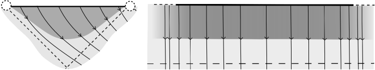
Figure 7: Schematic depiction of the development of perturbed initial data for the Schwarzschild-de Sitter spacetime and the congruence of conformal geodesics. In (a) the evolution of asymptotic initial data is depicted in the conformal representation in which the asymptotic points $\mathcal{Q}$ and $\mathcal{Q^{\prime}}$ are at a finite distance respect to the metric on $\mathscr{I}$. Figure (b) shows a schematic depiction of the evolution of asymptotic initial data in the conformal representation in which Theorem 1 has been formulated. In contrast to the conformal representation leading to Figure (a) , the initial data is homogeneous and formally identical for the subextremal, extremal or hyperextremal cases. In both diagrams, the dashed line corresponds to the location of an hypothetical Cauchy horizon of the development.

The main analysis of the background solution in Section 4.2 was performed in a conformal representation in which the asymptotic initial data is homogeneous and the extrinsic curvature of $\mathscr{I}$ vanishes —i.e. $\kappa=0$. The general evolution equations (38a)-(38b) consist of transport equations for ${\bm{\upsilon}}$ coupled with a system of partial differential equations for ${\bm{\phi}}$. However, as shown in Section 4.2, the assumption of spherical symmetry implies that the only independent component of the spinorial field $\phi_{{\bm{A}}{\bm{B}}{\bm{C}}{\bm{D}}}$ is $\phi_{2}$. Consequently, the system (38a)-(38b) reduces, for the background fields $\mathring{\mathbf{u}}=(\mathring{\bm{\upsilon}},\mathring{\bm{\phi}})$, to a system of ordinary differential equations. The Piccard-Lindelöf theorem can be applied to discuss local existence of the latter system. However, one does not have, a priori, control on the smallness of the existence time. To obtain statements concerning the existence time of the perturbed solution, we recall that the discussion of the evolution equations of Section 4.2 shows that the components of solution $\ring{\mathbf{u}}$ are regular for $\tau\in[0,\tau_{\circledcirc}]$ with $\tau_{\circledcirc}$ as given in equation (85), so that the guaranteed existence time is not arbitrarily small.

The analysis of the core system in Section 4.2 was restricted to the case $\kappa=0$, in which the conformal boundary has vanishing extrinsic curvature. In this case, we obtained an explicit existence time $\tau_{\circledcirc}$ for the solution to the conformal evolution equations. In contrast, the analysis given in Appendix B shows that in general, for $\kappa\neq 0$, the core system develops a singularity at finite $\tau_{\lightning}$. Since the results given in Section 4.2.4 for the conformal deviation equations hold not only for $\kappa=0$, but for any $\kappa$ as long as $\partial_{\psi}\kappa=0$, one has that the congruence of conformal geodesics is non-intersecting in the $\kappa\neq 0$ case as well. This shows that, the singularities in the core system in the case $\kappa\neq 0$ are not gauge singularities. The estimation for the existence time $\tau_{\circledcirc}$ in the $\kappa=0$ case along with the discussion of the reparametrisation of conformal geodesics given in Appendix B.3 can, in principle, be used to obtain an estimation for the existence time $\tau_{\otimes}$ in the case $\kappa\neq 0$.

In this section it is shown how one can exploit these observations, together with the theory for symmetric hyperbolic systems, to prove the existence of solutions to the general conformal evolution equations with the same existence time $\tau_{\circledcirc}$ for small perturbations of asymptotic initial data close to that of the Schwarzschild-de Sitter reference solution. By construction, the development of this perturbed data will be contained in the domain of influence which corresponds, in this case, to the asymptotic region of the spacetime —see Figure 7.

Taking into account the above remarks and using the theory of symmetric hyperbolic systems contained in [37] one can formulate the following existence and Cauchy stability result:

Theorem 1 (existence and Cauchy stability for perturbations of asymptotic initial data for the Schwarzschild-de Sitter spacetime).

Let $\mathbf{u}_{\star}=\ring{\mathbf{u}}_{\star}+\breve{\mathbf{u}}_{\star}$ denote asymptotic initial data for the extended conformal Einstein field equations on a 3-dimensional manifold $\mathcal{S}\approx\mathbb{R}\times\mathbb{S}^{2}$ where $\ring{\mathbf{u}}_{\star}$ denotes the asymptotic initial data for the Schwarzschild-de Sitter spacetime (subextremal, extremal and hyperextremal cases) with $\kappa=0$ in which the asymptotic points $\mathcal{Q}$ and $\mathcal{Q^{\prime}}$ are at infinity. Then, for $m\geq 4$ and $\tau_{\circledcirc}$ as given in equation (85), there exists $\varepsilon>0$ such that:

• for $||\breve{\mathbf{u}}_{\star}||_{\mathcal{S},m}<\varepsilon$ , there exist a unique solution $\breve{\mathbf{u}}$ to the conformal evolution equations (40a)-(40b) with a minimal existence interval $[0,\tau_{\circledcirc}]$ and

  $$\breve{\mathbf{u}}\in C^{m-2}([0,\tau_{\circledcirc}]\times\mathcal{S},\mathbb{C}^{N}),$$

  and the associated congruence of conformal geodesics contains no conjugate points in $[0,\tau_{\circledcirc}]$;

• given a sequence of perturbed data $\{\breve{\mathbf{u}}_{\star}^{(n)}\}$ such that

  $$\parallel\breve{\mathbf{u}}_{\star}^{(n)}\parallel_{\mathcal{S},m}\rightarrow 0\qquad\mbox{as}\qquad n\rightarrow\infty,$$

  then the corresponding solutions $\{\breve{\mathbf{u}}^{(n)}\}$ have a minimum existence interval $[0,\tau_{\circledcirc}]$ and it holds that

  $$\parallel\breve{\mathbf{u}}^{(n)}\parallel_{\mathcal{S},m}\rightarrow 0\qquad\mbox{as}\qquad n\rightarrow\infty$$

  uniformly in $\tau\in[0,\tau_{\circledcirc}]$ as $n\rightarrow\infty$;

• the solution $\mathbf{u}=\ring{\mathbf{u}}+\breve{\mathbf{u}}$ is unique in $[0,\tau_{\circledcirc}]\times\mathcal{S}$ and implies a $C^{m-2}$ solution $(\tilde{\mathcal{M}}_{\tau_{\circledcirc}},\tilde{{\bm{g}}})$ to the Einstein vacuum equations with the same de Sitter-like Cosmological constant as the background solution where

  $$\tilde{\mathcal{M}}_{\tau_{\bullet}}\equiv(0,\tau_{\circledcirc})\times\mathcal{S}.$$

  Moreover, the hypersurface $\mathscr{I}\equiv\{0\}\times\mathcal{S}$ represents the conformal boundary of the spacetime.

Proof.

Points (i) and (ii) are a direct application of the theory contained in [37] where it is used that the background solution $\ring{\mathbf{u}}$ is regular on $\tau\in[0,\tau_{\circledcirc}]$. The initial data for the Schwarzschild-de Sitter spacetime encoded in $\mathbf{u}_{\star}$ is in a representation in which the points $\mathcal{Q}$ and $\mathcal{Q^{\prime}}$ are at infinity. Observe that the asymptotic initial data, as derived in Section 3.5, for the subextremal, extremal and hyperextremal cases are formally the same —in particular, notice that the initial data for the electric part of the rescaled Weyl tensor contains information about the mass $m$ while the conformal factor $\Theta$ carries information about $\lambda$. The arguments in the analysis of Section 4.2 are irrespective of the relation between $\lambda$ and $m$. The key observation in the proof is that one can apply the general theory of symmetric hyperbolic systems of [37] for each open set and chart of an atlas for $\mathbb{R}\times\mathbb{S}^{2}$; then, these local solutions can be patched together to obtain the required global solution over $[0,\tau_{\circledcirc}]\times\mathcal{S}$ —it is sufficient to cover $\mathbb{R}\times\mathbb{S}^{2}$ with finitely many patches (two) as discussed in Section 4.3.2. Details of a similar construction in the context of characteristic problems can be found in [19]. To prove point (iii) first observe that from Lemma 5 the solution to the conformal evolution system (40a)-(40b) implies a solution $\mathbf{u}=\ring{\mathbf{u}}+\breve{\mathbf{u}}$ to the extended conformal Einstein field equations on $[0,\tau_{\circledcirc}]\times\mathcal{S}$ if $\mathbf{u}_{\star}=\ring{\mathbf{u}}_{\star}+\breve{\mathbf{u}}_{\star}$ solves the conformal constraint equations on the initial hypersurface. This solution implies, using Lemma 1, a solution to the Einstein field equations whenever the conformal factor is not vanishing. General results of the theory of asymptotics implies then that the initial hypersurface $\mathcal{S}$ can be interpreted as the conformal boundary of the physical spacetime $(\tilde{\mathcal{M}}_{\tau_{\bullet}},\tilde{{\bm{g}}})$ —see [51, 53]. ∎

5 Conclusions

In this article we have studied the Schwarzschild-de Sitter family of spacetimes as a solution to the extended conformal Einstein field equations expressed in terms of a conformal Gaussian system. Given that, in principle, it is not possible to explicitly express the spacetimes in this gauge, we have adopted the alternative strategy of formulating an asymptotic initial value problem for a spherically symmetric spacetime with a de Sitter-like Cosmological constant. The generalisation of Birkhoff’s theorem to vacuum spacetimes with Cosmological constant then ensures that the resulting solutions are necessarily a member of the Schwarzschild-de Sitter spacetime.

As part of the formulation of an asymptotic initial value problem for the Schwarzschild-de Sitter spacetime we needed to specify suitable initial data for the conformal evolution equations. The rather simple form that the conformal constraint equations acquire in the framework considered in this article allows to study in detail the conformal properties of the Schwarzschild-de Sitter spacetime at the conformal boundary and, in particular, at the asymptotic points where the conformal boundary meets the horizons. The key observation from this analysis is that the conformal structure is singular at these points and cannot be regularised in an obvious manner. Accordingly, any satisfactory formulation of the asymptotic initial value problem will exclude these points.

An interesting property of the conformal evolution equations under the assumption of spherical symmetry is that the system reduces to a set of transport equations along the conformal geodesics covering the spacetime. The essential dynamics, and in particular the formation of singularities in the solutions to this system, is governed by a core system of three equations —one of them a Riccati equation. As discussed in Appendix B, this core system provides a mechanism for the formation of singularities in the exact solution. The analysis of the core system allows not only to study the properties on the Schwarzschild-de Sitter spacetime expressed in terms of a conformal Gaussian gauge system, but also to understand the effects that the gauge data has on the properties of the conformal representation arising as a solution to the conformal evolution equations. It is of interest to explore the idea of whether the mechanisms identified in the analysis of the core system could be used to analyse the formation of singularities in more complicated spacetimes —say, in the developments of perturbations of asymptotic initial data for the Schwarzschild-de Sitter spacetime.

The conformal representation of the Schwarzschild-de Sitter spacetime obtained in this article has been used to show that it is possible to construct, say, future asymptotically de Sitter solutions to the Einstein vacuum Einstein with a minimum existence time —as measured by the proper time of the conformal geodesics used to construct the gauge system— which can be understood as perturbations of a member of the Schwarzschild-de Sitter family of spacetimes. As already mentioned in the main text, it is an interesting problem to determine the maximal Cauchy development to these spacetimes. In order to obtain the maximal Cauchy development of suitably small perturbations of asymptotic data for the Schwarzschild-de Sitter one would require the use of more refined methods of the theory of hyperbolic partial differential equations as one is, basically, confronted with global existence problem for the conformal evolution equations. In this respect, we conjecture that the time symmetric conformal representation in which $\kappa=0$ together with the global stability methods of [38] should allow us to make inroads into this issue. Closely related to the construction of the maximal development of perturbations of asymptotic initial data of the Schwarzschild-de Sitter spacetime is the question whether there is a Cauchy horizon associated to the boundary of this development. If this is the case, one would like to investigate the properties of this horizon. Intuitively, the answer to these issues should depend on the relation between the asymptotic points $\mathcal{Q}$ and $\mathcal{Q}^{\prime}$ and the conformal structure of the spacetime. In particular, one would like to know whether the singularities of the rescaled Weyl tensor at these points generically propagate along the boundary of the perturbed solution —notice, that they do not for the background solution. If one were able to use the $\mathbb{R}\times\mathbb{S}^{2}$-representation of the conformal boundary of perturbations of asymptotic initial data for the Schwarzschild-de Sitter to construct a maximal development and to gain sufficient control on the asymptotic behaviour of the various conformal fields, one could then rescale this solution to obtain a representation with a conformal boundary of the form $\mathbb{S}^{3}\setminus\{\mathcal{Q},\mathcal{Q}^{\prime}\}$. As discussed in the main text, in this representation some fields are singular at $\mathcal{Q}$ and $\mathcal{Q}^{\prime}$. This observation suggests that this construction could shed some light regarding the propagation (or lack thereof) of singularities near the asymptotic points $\mathcal{Q}$ and $\mathcal{Q}^{\prime}$.

Appendix A Appendix: The asymptotic points $\mathcal{Q}$ and $\mathcal{Q^{\prime}}$ and conformal geodesics in the Schwarzschild-de Sitter spacetime

A.1 Analysis of the asymptotic points $\mathcal{Q}$ and $\mathcal{Q^{\prime}}$

In Section 3.2 it was shown that there exist a conformal representation of the Schwarzschild-de Sitter spacetime in which the metric at the conformal boundary is ${\bm{\hbar}}$ —i.e. the standard metric on $\mathbb{S}^{3}$. In addition, we observed that the North and South pole of $\mathbb{S}^{3}$ correspond to special points in the conformal structure that we have labelled as $\mathcal{Q}$ and $\mathcal{Q^{\prime}}$. These asymptotic regions are represented in the Penrose diagram for the subextremal, extremal and hyperextremal Schwarzschild-de Sitter spacetime as the points where the conformal boundary and the Cosmological horizon, Killing horizon and singularity, respectively, seem to meet —see Figures 3 and 4 and 5. As discussed in Section 3.2 these points correspond to $(\bar{U},\bar{V})=(\pm\frac{\pi}{2},\pm\frac{\pi}{2})$ for which the tortoise coordinate $\mathfrak{r}$ is not well defined. In Section 3.4 we showed that in the conformal representation in which the initial metric is ${\bm{\hbar}}$ the data for the electric part of the rescaled Weyl tensor $\mathchar 22\relax\mkern-13.0mud_{{\bm{i}}{\bm{j}}}$, as given in equation (65), is singular precisely at $\mathcal{Q}$ and $\mathcal{Q^{\prime}}$. Observe that written in spinorial terms the initial data for the rescaled Weyl spinor in this conformal representation is given by

$$\mathchar 22\relax\mkern-13.0mu\phi_{{\bm{A}}{\bm{B}}{\bm{C}}{\bm{D}}}=\frac{6m}{\sqrt{1-\omega^{2}(\xi)}}\epsilon^{2}{}_{{\bm{A}}{\bm{B}}{\bm{C}}{\bm{D}}}$$

which is singular at both $\mathcal{Q}$ and $\mathcal{Q^{\prime}}$. This situation resembles that of the geometry near spacelike infinity $i^{0}$ of the Minkowski spacetime and the construction of the cylinder at infinity given in [22] which allows to regularise the data for the rescaled Weyl spinor. However, some experimentation reveals that this type of regularisation procedure (in contrast with the analysis of Schwarzschild spacetime given in [22]) cannot be implemented in the analysis of the Schwarzschild-de Sitter spacetime without spoiling the regular behaviour of the conformal factor. Since the hyperbolic reduction procedure for the extended conformal Einstein field equations is based on the existence of a congruence of conformal geodesics in spacetime, the singular behaviour of the initial data for the rescaled Weyl spinor suggest that the congruence of conformal geodesics does not cover the region of the spacetime corresponding to $\mathcal{Q}$ and $\mathcal{Q^{\prime}}$. To clarify this point, in the remaining of this section we analyse the behaviour of conformal geodesics as they approach the asymptotic points $\mathcal{Q}$ and $\mathcal{Q^{\prime}}$.

A.2 Geodesics in Schwarzschild-de Sitter spacetime

The method for the hyperbolic reduction for the extended conformal Einstein field equations available in the literature requires adapting the gauge to a congruence of conformal geodesics. The behaviour of metric geodesics in the Schwarzschild-de Sitter spacetime has been already studied [35, 34] and an analysis of conformal geodesics in Schwarzschild-de Sitter and anti-de-Sitter spacetimes is carried out in [30]. In static coordinates $(t,r,\theta,\varphi)$ the equation for radial timelike geodesics, $(\theta=\theta_{\star},\varphi=\varphi_{\star})$ with $\theta_{\star}$ and $\varphi_{\star}$ constant, are

$$\frac{\mbox{d}r}{\mbox{d}\tilde{\tau}}=\sqrt{\gamma^{2}-F(r)},\qquad\frac{\mbox{d}t}{\mbox{d}\tilde{\tau}}=\frac{\gamma}{F(r)}.$$ (91)

The first equation can be formally integrated as

$$\tilde{\tau}-\tilde{\tau}_{\star}=\int_{r_{\star}}^{r}\frac{1}{\sqrt{\gamma^{2}-F(s)}}\mbox{d}s$$ (92)

where $\tilde{\tau}$ is the $\tilde{{\bm{g}}}_{SdS}$-proper time and $\gamma$ is a constant of motion which can be identified with the specific energy of a particle moving along the geodesic. The equation for $t$ can be solved once equation (92) has been integrated. As pointed out in [7, 47], by choosing $\gamma=1$ one can explicitly solve this integral. However in general, for arbitrary $\gamma$, the integral is complicated and cannot be written in terms of elementary functions. A side observation is that if $r\neq r_{b}$ and $r\neq r_{c}$ then the curves of constant $t$ correspond to geodesics with $\gamma=0$. Finally, its worth noticing that geodesics with constant $r$ are characterised by the condition

$$\gamma^{2}-F(r)=0.$$ (93)

This last type of curves, which will be called critical curves, are analysed in Section A.4. In general, the properties of conformal geodesics differ from their metric counterparts. However, in the case of an Einstein spacetime with spacelike conformal boundary any conformal geodesic leaving $\mathscr{I}$ orthogonally is, up to reparametrisation, a metric geodesic — see [28] and Lemma 4.

A.3 A special class of conformal geodesics in the Schwarzschild-de Sitter spacetime

As briefly mentioned in Section A.2 and pointed out in [7, 47], in general, the integral (92) cannot be written in terms of elementary functions except for the the special case when $\gamma=1$ where it yields

$$r(\tilde{\tau})=\mathcal{C}e^{\tilde{\tau}}\left(1-\left(\frac{3m}{2|\lambda|}\right)\mathcal{C}^{-3}e^{-3\tilde{\tau}}\right)^{2/3},$$ (94)

where $\mathcal{C}$ is an integration constant. The last expression is valid irrespective of the relation between $m$ and $\lambda$. One can also use this expression to integrate the second equation in (91) to obtain the geodesic parametrised as $(r(\tilde{\tau}),t(\tilde{\tau}))$. The integration of $t$ will not be required for the purposes of the analysis of this section. A complete analysis of conformal geodesics in the Schwarzschild-de Sitter and anti-de Sitter spacetimes will be given in [30]. By virtue of Lemma 4 one can recast the geodesic with $\gamma=1$ as a conformal geodesic by reparametrising it in terms of the unphysical proper time as determined by equations (16) and (37). A straightforward computation yields

$$\tilde{\tau}(\tau)=\sqrt{\frac{3}{|\lambda|}}\ln\left\lvert\frac{\tau}{2+\kappa\tau}\right\rvert.$$ (95)

Equivalently, assuming either $\kappa>0$ and $\tau\geq 0$ or $\kappa<0$ and $0\leq\tau\leq-2/\kappa$ one obtains in both cases

$$\tau(\tilde{\tau})=\frac{2\exp\Big{(}\sqrt{\displaystyle\frac{|\lambda|}{3}}\tilde{\tau}\Big{)}}{1-\kappa\exp\Big{(}\sqrt{\displaystyle\frac{|\lambda|}{3}}\tilde{\tau}\Big{)}}.$$ (96)

From the last expression one can verify that

$$\lim_{\tilde{\tau}\rightarrow-\infty}\tau(\tilde{\tau})=0,\qquad\lim_{{\tau}\rightarrow\infty}\tau(\tilde{\tau})=-2/\kappa,$$

as expected. In what follows, we will rewrite equation (94) in terms of the unphysical proper time as

$$r(\tau)=\frac{1}{(m|\lambda|)^{2/3}}\frac{(m|\lambda|\mathcal{C}^{3}\tau^{3}-6(2+\kappa\tau)^{3})^{2/3}}{\mathcal{C}\tau(\tau+2\kappa\tau)}.$$ (97)

From the last expressions one can verify that one has $r\rightarrow\infty$ as $\tau\rightarrow 0$ and $\tau\rightarrow-2/\kappa$. The location of the singularity $r=0$ is determined by

$$\tau_{\lightning}=\frac{2}{(m|\lambda|)^{1/3}\mathcal{C}-\kappa}.$$

Recalling that $\mathcal{C}$ is an integration constant which depends on the initial data for the congruence, since the only freedom left in the conformal factor is encoded in $\kappa$, one realises that $\mathcal{C}=\mathcal{C}(\kappa)$. So one cannot draw any precise conclusion about the location of the singularity unless one further identifies explicitly $\mathcal{C}(\kappa)$. In particular, considering constant $\kappa$ as we have done for the analysis of the core system and setting $\mathcal{C}$ to be proportional to $\kappa$, say $\mathcal{C}=\frac{(2\varkappa+1)}{(m|\lambda|)^{1/3}}\kappa$ for some proportionality constant $\varkappa$, one obtains

$$\tau_{\lightning}=\frac{1}{\varkappa\kappa},$$

which is in agreement the with the qualitative behaviour of the core system as shown in Figures 6, 9, and 10. Notice, however, that the arguments of the core system given in Section 4.2.2 and Appendix B do not rely on integrating (92) explicitly as we have done in this section.

A.4 Critical curves on the Schwarzschild-de Sitter spacetime

In order to clarify the role of the asymptotic points, in this section we show that there are not timelike conformal geodesics reaching $\mathcal{Q}$ and $\mathcal{Q^{\prime}}$ orthogonally. More precisely, we show that a timelike conformal geodesic becomes asymptotically null as it approaches $\mathcal{Q}$ and $\mathcal{Q^{\prime}}$. This is in stark tension with the required conditions for constructing a conformal Gaussian system of coordinates in the neighbourhood of $\mathcal{Q}$ and $\mathcal{Q^{\prime}}$.

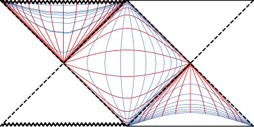
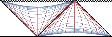
Figure 8: Curves of constant $r$ and $t$ in the Schwarzschild-de Sitter spacetime. a) Curves with constant $t$ and $r$ (red and blue respectively) are plotted on the Penrose diagram of the Subextremal Schwarzschild-de Sitter spacetime. Curves of constant $t$ accumulate at the bifurcation spheres $\mathcal{B}$, $\mathcal{B^{\prime}}$ while the curves of constant $r$ accumulate at the asymptotic points $\mathcal{Q}$ and $\mathcal{Q^{\prime}}$. b) Curves with constant $t$ and $r$ (red and blue respectively) are plotted on the Penrose diagram of the extremal Schwarzschild-de Sitter spacetime. In contrast with the subextremal case, curves with constant $t$ in starting from some $r_{\star}<3m$ accumulate at the asymptotic points $\mathcal{Q}$ and $\mathcal{Q^{\prime}}$ while those starting from $r_{\star}>3m$ accumulate at $\mathcal{P}$. The hyperextremal case is qualitatively similar to the extremal one and has been omitted.

As shown in the Penrose diagram of Figure, 8 in the subextremal case the curves of constant $t=t_{\star}$ accumulate in the bifurcation spheres $\mathcal{B}$ and $\mathcal{B^{\prime}}$ while the curves of constant $r$ accumulate in the asymptotic points $\mathcal{Q}$ and $\mathcal{Q^{\prime}}$. By contrast, in the extremal case the curves with constant $t=t_{\star}$ approach the asymptotic points $\mathcal{Q}$ and $\mathcal{Q^{\prime}}$ —see [32] for an extensive discussion on the Penrose diagram for Schwarzschild-de Sitter spacetime. It follows from the geodesic equation (91) that the curves of constant $r$ correspond to geodesics whenever the condition (93) is satisfied, this equation explicitly reads

$$|\lambda|r^{3}+3(\gamma^{2}-1)r+6m=0.$$ (98)

Observe that for $\gamma=1$ the last condition reduces to $|\lambda|r^{3}+6m=0$ which cannot be solved for positive $r$.

In this section we perform an analysis of the behaviour of the critical curves on the Schwarzschild-de Sitter spacetime. Notice that in the hyperextremal case the are no timelike geodesics with constant $r$ since for $|\lambda|>1/9m^{2}$ one has strictly $F(r)<0$ so that the condition (93) can never be satisfied.

A.4.1 Critical curves in the extremal Schwarzschild-de Sitter spacetime

We start the analysis in the simpler case in which $|\lambda|=1/9m^{2}$ so that $F(r)$ is given as in equation (46) and the condition (93) reduces to considering $r=3m$ and $\gamma=0$. Observe that the curves with $\gamma=0$ and $r\neq 3m$ correspond to curves with constant $t=t_{\star}$ which, as discussed in previous paragraphs, approach asymptotically the points $\mathcal{Q}$ and $\mathcal{Q^{\prime}}$. Notice that for $\gamma=0$ the expression (92) can easily be integrated to yield

$$\tilde{\tau}-\tilde{\tau}_{\star}=3m\ln\left(H(r)/H(r_{\star})\right)$$ (99)

where

$$H(r)\equiv\frac{\sqrt{3r}+\sqrt{r+6m}}{(\sqrt{3r}-\sqrt{r+6m})(\sqrt{r}+\sqrt{r+6m})^{2\sqrt{3}}}.$$

Observe that equation (99), as pointed out in [47], implies that the geodesics with $\gamma=0$ never cross the horizon since $\tilde{\tau}\rightarrow\infty$ as $r\rightarrow 3m$. For simplicity, let $M_{\star}\equiv H(r_{\star})+\exp(\tilde{\tau}_{\star}/3m)$ with $r_{\star}\neq 3m$ so that $\tilde{\tau}=3m\ln|H(r)/M_{\star}|$. Reparametrising using equation (96) and that $|\lambda|=1/9m^{2}$ renders

$$\tau(r)=\frac{2W(r)}{M_{\star}^{p}-\kappa W(r)}$$

with $W(r)=H(r)^{1/\sqrt{3}}$. Using L’Hôpital rule one can verify that $\tau\rightarrow-2/\kappa$ as $r\rightarrow 3m$. To analyse the behaviour of these curves as they approach the points $\mathcal{Q}$ and $\mathcal{Q^{\prime}}$ let us consider $r$ such that $r=3m+\epsilon$ . Then, one has that for small $\epsilon>0$ that

$$W(r)=\left(\frac{m}{r-3m}\right)^{1/\sqrt{3}}\left(\frac{C_{1}}{m}+\frac{C_{2}}{m^{2}}(r-3m)+\mathcal{O}((r-3m)^{2})\right)$$

where $C_{1}$ and $C_{2}$ are numerical factors whose explicit form is not relevant for the subsequent discussion. Hence, to leading order $W(r)=C/\epsilon^{p}$ where $C$ is a constant depending on $m$ only and $p=1/\sqrt{3}$. Consequently, to leading order

$$\frac{\mbox{d}\tau}{\mbox{d}\epsilon}=-\frac{pC\kappa\epsilon^{p-2}}{\left(M_{\star}^{p}\epsilon^{p}-\kappa C\right)}-\frac{pC\epsilon}{M_{\star}^{p}\epsilon^{p}-\kappa C}.$$

Therefore, since $p<2$ one has that ${\mbox{d}\tau}/{\mbox{d}\epsilon}$ diverges as $\epsilon\rightarrow 0$ so that the curves with $\gamma=0$ become tangent to the horizon as they approach $\mathcal{Q}$ or $\mathcal{Q^{\prime}}$ —that is, they would have to become null to reach $\mathcal{Q}$ or $\mathcal{Q^{\prime}}$. This is analogous to the behaviour of the critical curve in the Schwarzschild spacetime pointed out in [23], and the subextremal Reissner-Nordström spacetime in [42] —in contrast, in the extremal Reissner-Nordström spacetime one has $\frac{\mbox{d}\tau}{\mbox{d}\epsilon}=0$ as $\epsilon\rightarrow 0$ as discussed in [42] .

A.4.2 Critical curves in the subextremal Schwarzschild-de Sitter spacetime

For the subextremal case one could parametrise the roots of the depressed cubic (98) using Vieta’s formulae and choose some $\gamma\neq 1$ for which there is at least one positive root. However, notice that fixing a value for $\gamma$ is equivalent to prescribe initial data for the congruence:

$$t(\tilde{\tau})=t_{\star},\qquad r(\tilde{\tau})=r_{\star},\qquad\frac{\mbox{d}r}{\mbox{d}\tilde{\tau}}\Big{\rvert}_{r_{\star}}=\sqrt{\gamma^{2}-F(r_{\star})},\qquad\frac{\mbox{d}t}{\mbox{d}\tilde{\tau}}\Big{\rvert}_{r_{\star}}=\frac{\gamma}{F(r_{\star})}.$$ (100)

Restricting our analysis to the static region $r_{b}<r_{\star}<r_{c}$ for which $F(r_{\star})>0$ and setting

$$\frac{\mbox{d}r}{\mbox{d}\tilde{\tau}}\Big{\rvert}_{r_{\star}}=0,$$

one gets

$$\gamma=\sqrt{F(r_{\star})},$$

and condition (93) is equivalent to

$$F(r_{\star})-F(r)=\frac{|\lambda|(r-r_{\star})}{3r}Q(r),$$

where $Q(r)$ is the polynomial

$$Q(r)\equiv r^{2}+r_{\star}r-\frac{6m}{|\lambda|r_{\star}}.$$

Notice that $Q(r)$ can be factorised as

$$Q(r)=(r-\alpha_{-}(r_{\star}))(r-\alpha_{+}(r_{\star})),$$

where

$$\alpha_{\pm}(r_{\star})\equiv\frac{r_{\star}}{2}\left(-1\pm\sqrt{1+\frac{24m}{|\lambda|r_{\star}^{3}}}\right).$$

In addition, observe that

$$Q(r_{\star}) > 0\qquad\text{for}\qquad r_{\circledast}<r_{\star}<r_{c},$$

$$Q(r_{\star}) < 0,\qquad\text{for}\qquad r_{b}<r_{\star}<r_{\circledast},$$

$$Q(r_{\star}) = 0,\qquad\text{for}\qquad r_{\star}=r_{\circledast},$$

where $r_{\circledast}\equiv\left(\frac{3m}{|\lambda|}\right)^{1/3}$. In the extremal case one has $r_{b}=r_{c}=r_{\circledast}=3m$. The curve $r=r_{\circledast}$, as in the extremal case, will be called the critical curve. With the above notation the integral (92) can be then rewritten as

$$\tilde{\tau}-\tilde{\tau}_{\star}=\int^{r}_{r_{\star}}\sqrt{\frac{s}{(s-r_{\star})(s-\alpha_{-}(r_{\star}))(s-\alpha_{+}(r_{\star}))}}\mbox{d}s.$$ (101)

To study the behaviour close to the critical curve consider $r_{\star}=(1+\epsilon)r_{\circledast}$ For small $\epsilon>0$ and considering $s>r_{\star}$ one can expand the right hand side of equation (101) in Taylor series as

$$\tilde{\tau}-\tilde{\tau}_{\star}=\int_{r_{\star}}^{r}\sqrt{\frac{s}{s+2r_{\circledast}}}\left(\frac{1}{s-r_{\circledast}}-\frac{3r_{\circledast}^{2}s\epsilon^{2}}{2(s-r_{\circledast})^{3}}\right)\mbox{d}s+\mathcal{O}(\epsilon^{3}).$$ (102)

Integrating we obtain

$$\tilde{\tau}-\tilde{\tau}_{\star}=-\frac{2}{\sqrt{3}}\text{arctanh}\left(\sqrt{3}\sqrt{\frac{1+\epsilon}{3+\epsilon}}\right)+2\ln\left(\sqrt{r_{\circledast}(1+\epsilon)}+\sqrt{r_{\circledast}(3+\epsilon)}\right)-\frac{2}{\sqrt{3}}\text{arctanh}\left(\frac{3r}{r+2r_{\circledast}}\right)$$

$$+2\ln\left(\sqrt{r}+\sqrt{r+2r_{\circledast}}\right)\ -\frac{3}{4}r_{\circledast}\sqrt{1+2r_{\circledast}}(1+2\epsilon)-\frac{3}{4}r_{\circledast}{}^{2}\sqrt{1+2r_{\circledast}}\frac{(2r-r_{\circledast})\epsilon^{2}}{(r_{\circledast}-r)^{2}}+\mathcal{O}(\epsilon^{3}).$$

As $\epsilon\rightarrow 0$ the last expression diverges —as is to be expected. The divergent term can be expanded for small $\epsilon>0$ as

$$\text{arctanh}\left(\sqrt{3}\sqrt{\frac{1+\epsilon}{3+\epsilon}}\right)=\frac{1}{2}\ln\left(\left\lvert-\frac{6}{\epsilon}+4+\frac{\epsilon}{6}+\mathcal{O}(\epsilon^{2})\right\rvert\right)$$

and the second term can be expanded as

$$\ln\left(\sqrt{r_{\circledast}(1+\epsilon)}+\sqrt{r_{\circledast}(3+\epsilon)}\right)=\ln\left((1+\sqrt{3})\sqrt{r_{\circledast}}\right)+\frac{\epsilon}{2\sqrt{3}}-\frac{\epsilon^{2}}{6\sqrt{3}}+\mathcal{O}(\epsilon^{3}).$$

Hence, to leading order one has

$$\tilde{\tau}(r)=\frac{1}{\sqrt{3}}\ln\epsilon+f(r)+\mathcal{O}(\epsilon)$$

where

$$f(r)=\tilde{\tau}_{\star}+2\ln\left((1+\sqrt{3})\sqrt{r_{\circledast}}\right)-\frac{2}{\sqrt{3}}\text{arctanh}\left(\frac{3r}{r+2r_{\circledast}}\right)\\ +2\ln\left(\sqrt{r}+\sqrt{r+2r_{\circledast}}\right)\ -\frac{3}{4}r_{\circledast}\sqrt{1+2r_{\circledast}}.$$

Reparametrising respect to the unphysical proper time using (96) one gets

$$\tau(r)=\frac{2\exp\left(\sqrt{|\lambda|/3}f(r)+\mathcal{O}(\epsilon)\right)\epsilon^{p}}{1-\kappa\exp\left(\sqrt{|\lambda|/3}f(r)+\mathcal{O}(\epsilon)\right)\epsilon^{p}}$$

with $p=1/\sqrt{3}$. Thus one gets

$$\frac{\mbox{d}\tau}{\mbox{d}\epsilon}=\frac{2p\exp\left(\sqrt{|\lambda|/3}f(r)+\mathcal{O}(\epsilon)\right)\epsilon^{p-1}}{\left(1-\exp\left(\sqrt{|\lambda|/3}f(r)+\mathcal{O}(\epsilon)\right)\kappa\epsilon^{p}\right)^{2}}.$$

Observe that since $p<1$ then one has that $\mbox{d}\tau/\mbox{d}\epsilon$ diverges as $\epsilon\rightarrow 0$.

Appendix B Appendix: The conformal evolution equations in the case $\kappa\neq 0$ and reparametrisations

In Section 4.2.2 we analysed the case $\kappa=0$ —this corresponds to a conformal boundary with vanishing extrinsic curvature. Nevertheless, as discussed in Section 2.4, $\kappa$ is a conformal gauge quantity arising from the conformal covariance of the conformal field equations. Consequently, it is of interest to analyse the behaviour of the core system in the case $\kappa\neq 0$. For simplicity, in the remainder of this section, $\kappa$ will be assumed to be a constant on the initial hypersurface corresponding to $\tau=0$. In first instance, we restrict our attention to $|\kappa|>1$ and then discuss how to exploit the conformal covariance of the equations to extend these results for $\kappa\in[-1,0)\cup(0,1]$.

B.1 Analysis of the core system with $\kappa>1$

We begin the discussion of this case observing that, for $\kappa>1$, one has that $\Theta(\tau)\geq 0$ and $\dot{\Theta}(\tau)>0$ for $\tau\geq 0$. Using this simple observation and the core equations (73a)-(73c) we obtain the following:

Lemma 14.

For a solution to the core system (73a)-(73c) with initial data given by (74) and $\kappa>1$ one has that $L(\tau)<0$ for $\tau\geq 0$.

Proof.

We proceed by contradiction. Assume that there exists $0<\tau_{L}<\infty$ such that $L(\tau_{L})=0$. Without loss of generality we can assume that $\tau_{L}$ corresponds to the first zero of $L(\tau)$. Since for $\kappa>1$ we have $L(0)<0$ then by continuity it follows that $\dot{L}(\tau_{L})\geq 0$ —$\dot{{L}}(\tau_{L})$ cannot be negative since this would imply that ${L}(\tau)$ crossed the $\tau$-axis at some time $\tau<\tau_{L}$ but this is not possible since $\tau_{L}$ is the first zero of ${L}(\tau)$. It follows then from equation (73c) that

$$0\leq\dot{L}(\tau_{L})=-\chi(\tau_{L})L(\tau_{L})-\frac{1}{2}\dot{\Theta}(\tau_{L})\phi(\tau_{L}).$$

Since $L(\tau_{L})=0$ and $\dot{\Theta}(\tau_{L})>0$, the last inequality implies that $\phi(\tau_{L})\leq 0$ but this is a contradiction since we already know from Observation 1 that $\phi(\tau)>0$ for any $\tau$. ∎

Observation 4. Using that $\dot{\Theta}(\tau)\geq 0$ for $\kappa>1$ and $\tau\geq 0$ and that $\phi(\tau)>0$ we obtain from equation (73c) the differential inequality

$$\dot{L}(\tau)\leq-\chi(\tau)L(\tau).$$

Observing Lemma 14 we have that $L(\tau)<0$. Thus, we can formally integrate the last differential inequality and obtain

$$L(\tau)\leq L(0)\exp\left(-\int^{\tau}_{0}\chi(\mbox{s})\mbox{d}\mbox{s}\right).$$ (103)

We now show that the function $\chi(\tau)$ which is initially positive must necessarily have a zero.

Lemma 15.

For a solution to the core system (73a)-(73c) with initial data given by (74) and $\kappa>1$ there exist $0<\tau_{\chi}<\infty$ such that $\chi(\tau_{\chi})=0$.

Proof.

We proceed again by contradiction. Assume that $\chi(\tau)$ never vanishes. Since $\chi(0)=\kappa>0$ then $\chi(\tau)>0$ for $\tau\geq 0$. From Lemma 14 we know that $L(\tau)<0$. In addition, we know that $\Theta(\tau)\phi(\tau)\geq 0$. With these observations equation (73b) gives

$$\dot{\chi}(\tau)<-\chi^{2}(\tau)\hskip 14.22636pt\text{for}\hskip 14.22636pt\tau>0.$$

Since we are assuming that $\chi(\tau)$ never vanishes then

$$\frac{\dot{\chi}(\tau)}{\chi^{2}(\tau)}<-1.$$

Integrating from $0$ to $\tau>0$ and using the initial data (74) we get

$$\chi(\tau)<\frac{1}{\tau+{1}/{\kappa}}\hskip 14.22636pt\text{for}\hskip 14.22636pt\tau>0.$$ (104)

In a similar way, we can consider equation (73b) and obtain the differential inequality

$$\dot{\chi}(\tau)<-\frac{1}{2}\Theta(\tau)\phi(\tau)\hskip 14.22636pt\text{for}\hskip 14.22636pt\tau\geq 0.$$

Using now equation (75) we get

$$\dot{\chi}<-m\Theta(\tau)\exp\left({-3\int^{\tau}_{0}\chi(\mbox{s})\mbox{d}\mbox{s}}\right)\hskip 14.22636pt\text{for}\hskip 14.22636pt\tau\geq 0.$$

Integrating the from $0$ to $\tau>0$ we get

$$\chi(\tau)<\kappa-m\int^{\tau}_{0}\Theta(\mbox{s})\exp\left({-3\int^{s}_{0}\chi(\mbox{s}^{\prime})\mbox{ds}^{\prime}}\right)\mbox{ds}\hskip 14.22636pt\text{for}\hskip 14.22636pt\tau\geq 0.$$ (105)

On the other hand, integrating expression (104) we have

$$\int^{\tau}_{0}\chi(\mbox{s})\mbox{ds}<\ln\left(\kappa\tau+1\right).$$

Consequently,

$$-m\Theta(\tau)\exp\left({-3\int^{\tau}_{0}\chi(\mbox{s}^{\prime})\mbox{ds}^{\prime}}\right)<-m\sqrt{\frac{|\lambda|}{3}}\frac{\tau(1+\tfrac{1}{2}\kappa\tau)}{(1+\kappa\tau)^{3}}.$$

Integrating we get

$$-m\int^{\tau}_{0}\Theta(\mbox{s})\exp\left({-3\int^{s}_{0}\chi(\mbox{s}^{\prime})\mbox{ds}^{\prime}}\right)\mbox{ds}<-\frac{m}{2\kappa^{2}}\sqrt{\frac{|\lambda|}{3}}\left(\frac{1}{(\kappa\tau+1)^{2}}+\ln(\kappa\tau+1)-1\right).$$

Substituting the above result into the inequality (105) we obtain

$$\chi(\tau)<\kappa-\frac{m}{2\kappa^{2}}\sqrt{\frac{|\lambda|}{3}}\left(\frac{1}{(\kappa\tau+1)^{2}}+\ln(\kappa\tau+1)-1\right).$$

The right hand side of the last expression becomes negative for some sufficiently large $\tau$. This is a contradiction as we have assumed that $\chi(\tau)$ never vanishes and $\chi(0)>0$. ∎

Observation 5. Combining Lemma 14 and Observation 1, we conclude that $L(\tau)<0$ and $\Theta(\tau)\phi(\tau)>0$ for $\tau>0$. Using these properties in equation (73b) we get

$$\dot{\chi}(\tau)<0\hskip 14.22636pt\text{for}\hskip 14.22636pt\tau\geq 0.$$

Thus, $\chi(\tau)$ is always decreasing. From Lemma 15 we know that there exists a finite $\tau_{\chi}>0$ such that $\chi(\tau_{\chi})=0$. Then, by continuity, for any $\tau>\tau_{\chi}$ we have that $\chi(\tau)<0$ .

With this last observation we are in the position of proving the main result of this section:

Proposition 1.

There exists $0<\tau_{\lightning}<\infty$ such that the solution of (73a)-(73c) with initial data given by (74) and $\kappa>1$ satisfies

$$\chi\rightarrow-\infty,\quad L\rightarrow-\infty,\quad\phi\rightarrow\infty\quad\mbox{as}\quad\tau\rightarrow\tau_{\lightning}.$$

Proof.

From Lemma 15 we know there exists a finite $\tau_{\chi}$ for which $\chi(\tau)$ vanishes. By Observation 5, we have that $\chi(\tau_{\lozenge})<0$ for any $\tau_{\lozenge}>\tau_{\chi}$. Let $\chi_{\lozenge}\equiv\chi(\tau_{\lozenge})<0$. We can assume that $\chi_{\lozenge}$ is finite, otherwise there is nothing to prove. Now, using Lemma 14 and that $\Theta(\tau)\phi(\tau)>0$ we get

$$\dot{\chi}(\tau)<-\chi^{2}(\tau)\hskip 14.22636pt\text{for}\hskip 14.22636pt\tau\geq 0.$$

Since we know that $\chi(\tau)<0$ for any $\tau>\tau_{\lozenge}$ then

$$\frac{\dot{\chi}(\tau)}{\chi^{2}(\tau)}<-1.$$

Integrating form $\tau=\tau_{\lozenge}$ to $\tau>\tau_{\lozenge}$ we get

$$\chi(\tau)<\frac{1}{\tau-\tau_{\lozenge}+{1}/{\chi_{\lozenge}}}\hskip 14.22636pt\text{for}\hskip 14.22636pt\tau>\tau_{\lozenge}.$$ (106)

From inequality (106) we can conclude that $\chi(\tau)\rightarrow-\infty$ for some finite time $\tau_{\lightning}<\tau_{\lozenge}-{1}/\chi_{\lozenge}$. Additionally, observe that $\tau_{\lozenge}-{1}/{\chi_{\lozenge}}>\tau_{\lozenge}>0$ since $\chi_{\lozenge}<0$ . Now, given that $\chi\rightarrow-\infty$ as $\tau\rightarrow\tau_{\lightning}$ it follows from equation (75) that $\phi\rightarrow\infty$ as $\tau\rightarrow\tau_{\lightning}$. Similarly, from inequality (103) and that $L(0)<0$ it follows that $L\rightarrow-\infty$ as $\tau\rightarrow\tau_{\lightning}$. ∎

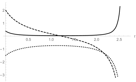
Figure 9: Numerical solutions of the core system (73a)-(73c) with initial data given by (74) in the case $\kappa=2$ and $|\lambda|=3$, $m=1/3\sqrt{3}$. The solid line describes the evolution of $\phi$, the dashed line that of $\chi$ and the dotted line that of $L$. One can observe the formation of a singularity at $\tau\approx 2.6392$.

Remark 10.

A plot of the numerical evaluation of the solutions to the core system (73a)-(73c) with initial data (74) in the case $\kappa>1$ can be seen in Figure 9.

B.2 Analysis of the core system with $\kappa<-1$

In this section we use a similar approach to that followed in Section B.1 to show that the fields in the core system diverge for some finite time if $\kappa<-1$. An interesting feature of this case is that, assuming one knows that there exists a singularity in the development, there exists an a priori upper bound for the time of its appearance —namely, the location of second component of the conformal boundary at $\tau=2/|\kappa|$. As a byproduct of the analysis of this section an improvement of this basic bound is obtained.

An important remark concerning the case $\kappa<-1$ is that if $\tau\in[0,1/|\kappa|]$ then both $\Theta(\tau)$ and $\dot{\Theta}(\tau)$ are non-negative. Based on this observation our first result is:

Lemma 16.

If $\kappa<-1$ then the solution to the core system (73a)-(73c) with initial data (74) satisfies $L(\tau)<0$ for $\tau\in[0,1/|\kappa|]$.

Proof.

We proceed by contradiction. Assume that there exists $0<\tau_{L}\leq 1/|\kappa|$ such that $L(\tau_{L})=0$. Without lost of generality we can assume that $\tau_{L}$ is the first zero of $L(\tau)$. Since $L(0)<0$ for $\kappa<-1$ then by continuity $\dot{L}(\tau_{L})\geq 0.$ Therefore, proceeding as in Lemma 14 one gets from (73c)

$$0\leq\dot{L}(\tau_{L})=-\chi(\tau_{L})L(\tau_{L})-\frac{1}{2}\dot{\Theta}(\tau_{L})\phi(\tau_{L})\hskip 14.22636pt\text{for}\hskip 14.22636pt\tau\in[0,1/|\kappa|].$$

Since $L(\tau_{L})=0$ and $\dot{\Theta}(\tau_{L})>0$ the last inequality implies that $\phi(\tau_{L})\leq 0$. This is a contradiction since $\phi(\tau)>0$ —cfr. Observation 1. ∎

Lemma 17.

If $\kappa<-1$ then the solution to the core system (73a)-(73c) with initial data (74) satisfies $\chi(\tau)<0$ for $\tau\in[0,1/|\kappa|]$.

Proof.

Again, we proceed by contradiction. Assume that there exists $0<\tau_{\chi}\leq 1/|\kappa|$ such that $\chi(\tau_{\chi})=0$. Without lost of generality we can assume that $\tau_{\chi}$ is the first zero of $\chi(\tau)$. Then, by continuity, we have that $\dot{\chi}(\tau_{\chi})\geq 0$. Using equation (73b) one has

$$0\leq\dot{\chi}(\tau_{\chi})=-\chi(\tau_{\chi})^{2}+L(\tau_{\chi})-\frac{1}{2}\Theta(\tau_{\chi})\phi(\tau_{\chi})\hskip 14.22636pt\text{for}\hskip 14.22636pt\tau\in[0,1/|\kappa|].$$

Therefore, since $\chi(\tau_{\chi})=0$ one has

$$L(\tau_{\chi})\geq\frac{1}{2}\Theta(\tau_{\chi})\phi(\tau_{\chi})>0.$$

This is a contradiction since by Lemma 16 we know that $L(\tau)<0$ for $\tau\in[0,1/|\kappa|]$. ∎

Observation 6. Proceeding as in Observation 4 one readily has that for $\kappa<-1$

$$L(\tau)\leq L(0)\exp\left(-\int_{0}^{\tau}\chi(\mbox{s})\mbox{ds}\right)\text{\hskip 14.22636pt for \hskip 14.22636pt}\tau\in(0,1/|\kappa|].$$

This last observation is used, in turn, to prove the main result of this section:

Proposition 2.

If $\kappa<-1$, then for the solution of (73a)-(73c) with initial data (74) there exists $0<\tau_{\lightning}<1/|\kappa|$ such that

$$\chi(\tau)\rightarrow-\infty,\quad L(\tau)\rightarrow-\infty,\quad\mbox{and}\quad\phi(\tau)\rightarrow\infty\quad\mbox{as}\quad\tau\rightarrow\tau_{\lightning}.$$

Proof.

Consider equation (73b) on the interval $\tau\in[0,1/|\kappa|]$. Using Lemma 16 we know that $L(\tau)<0$. This observation and the fact that $\phi(\tau)>0$ leads to the differential inequality

$$\dot{\chi}(\tau)<-\chi^{2}(\tau)\hskip 14.22636pt\text{for}\hskip 14.22636pt\tau\in[0,1/|\kappa|].$$

Since by Lemma 17, we know that $\chi(\tau)\neq 0$ for $\tau\in[0,1/|\kappa|]$ we can rewrite the last expression as

$$\frac{\dot{\chi}(\tau)}{\chi^{2}(\tau)}<-1\hskip 14.22636pt\text{for}\hskip 14.22636pt\tau\in[0,1/|\kappa|].$$

Integrating from $\tau=0$ to $1/|\kappa|$ and using the initial data (74) we get

$$\chi(\tau)<\frac{1}{\tau}-\frac{1}{|\kappa|}.$$ (107)

From inequality (107) one concludes that $\chi(\tau)\rightarrow-\infty$ for some $0<\tau_{\lightning}\leq 1/|\kappa|$. Finally, using Observation 6 and Observation 1 one concludes that $L(\tau)\rightarrow-\infty$ and $\phi(\tau)\rightarrow\infty$ as $\tau\rightarrow\tau_{\lightning}$ for some $0<\tau_{\lightning}\leq 1/|\kappa|$. ∎

Notice that this upper bound for the location of the singularity is not trivial and improves the basic bound $\tau\leq 2/|\kappa|$ given by the location of the second component of the conformal boundary.

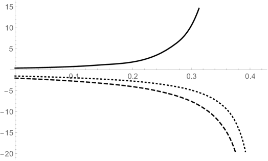
Figure 10: Numerical solution of the core system (73a)-(73c) with $|\lambda|=3$, $m=1/3\sqrt{3}$ in the case $\kappa=-2$. The solid line corresponds to $\phi$, the dashed line to $\chi$ and the dotted line to $L$. One can observe a singularity at $\tau\approx 0.4203$.

Remark 11.

A plot of the numerical evaluation of the solutions to the core system (73a)-(73c) with initial data (74) in the case $\kappa<-1$ can be seen in Figure 10.

B.3 Exploiting the conformal gauge

In Lemma 12 we have shown that if $\partial_{\psi}\kappa=0$ then the evolution equations imply, in particular, $f_{x}=0$. Due to the spherical symmetry Ansatz, the component $f_{x}$ is the only potentially non-zero component of ${\bm{f}}$. Thus, one concludes that ${\bm{f}}=0$. In Section B.3.1 we will exploit this feature of the Weyl connection to extract further information about $\kappa$ and $s$. These results are used in Section B.3.2 to discuss the conformal gauge freedom of the extended conformal field equations and the role played by reparametrisations of conformal geodesics.

B.3.1 The relation between the Weyl and Levi-Civita connections

As discussed in Section 2.2.1, the Weyl connection $\hat{{\bm{\nabla}}}$ expressing the extended conformal field equations is related to the Levi-Civita connection ${\bm{\nabla}}$ of the unphysical metric ${\bm{g}}$ via the 1-form ${\bm{f}}$. If ${\bm{f}}$ vanishes then $\hat{{\bm{\nabla}}}={\bm{\nabla}}$. Exploiting this simple observation we obtain the following results:

Lemma 18.

If ${\bm{f}}=0$ then the conformal gauge conditions (12) and (13) imply that $s=\ddot{\Theta}$. Moreover, $s$ is constant along the conformal geodesics.

Proof.

As discussed in Section 2.2.1 if ${\bm{f}}=0$ then $\hat{L}_{ab}=L_{ab}$ and $\hat{\Gamma}_{{\bm{a}}}{}^{{\bm{c}}}{}_{{\bm{b}}}=\Gamma_{{\bm{a}}}{}^{{\bm{c}}}{}_{{\bm{b}}}$. Using the conformal gauge condition (12) it follows that $L_{\bm{0}{\bm{a}}}=0$ and $\Gamma_{\bm{0}}{}^{{\bm{a}}}{}_{{\bm{b}}}=0$. Now, the standard conformal field equations (124d) and (124e) in Appendix D give

$$\nabla_{\bm{0}}\nabla_{\bm{0}}\Theta+\Theta L_{\bm{0}\bm{0}}-s\eta_{\bm{0}\bm{0}}=0,$$ (108a)

$$\nabla_{\bm{0}}s=-L_{\bm{0}{\bm{b}}}\nabla^{{\bm{b}}}\Theta.$$ (108b)

Using $L_{\bm{0}{\bm{a}}}=0$ and $\Gamma_{\bm{0}}{}^{{\bm{a}}}{}_{{\bm{b}}}=0$ in equation (108a) one concludes $\ddot{\Theta}=s$. Similarly, from equation (108b) one gets $\dot{s}=0$. Therefore $s$ is constant along the conformal geodesics. ∎

Remark 12.

In the asymptotic initial value problem the initial value of $s$ is given by $s_{\star}=\sqrt{|\lambda|/3}\kappa$ —see equation (34a). Thus, if ${\bm{f}}=0$ then $s=\sqrt{|\lambda|/3}\kappa$ along the conformal geodesics.

Finally, one has the following:

Lemma 19.

In the asymptotic initial value problem, if ${\bm{f}}=0$, then the conformal gauge conditions (12) and (13) together with the conformal Einstein field equations imply that ${\bm{e}}_{{\bm{i}}}(\kappa)=0$ —that is, $\kappa$ is a constant.

Proof.

Using ${\bm{f}}=0$ and the gauge conditions (12) we get from the conformal field equation (124g) that

$$6\Theta s-3\dot{\Theta}^{2}+3\delta^{{\bm{i}}{\bm{j}}}{\bm{e}}_{{\bm{i}}}\Theta{\bm{e}}_{{\bm{j}}}\Theta=\lambda.$$ (109)

Using Lemma 18 we have $s=\ddot{\Theta}$. Therefore, substituting $\Theta(\tau)=\dot{\Theta}_{\star}\tau(1+\kappa\tau/2)$ into equation (109) and recalling $\dot{\Theta}_{\star}=\sqrt{|\lambda|/3}$ we obtain

$$\tau^{4}\delta^{{\bm{i}}{\bm{j}}}{\bm{e}}_{{\bm{i}}}(\kappa){\bm{e}}_{{\bm{j}}}(\kappa)=0.$$

Observe that the last equation is trivially satisfied on $\mathscr{I}$ as $\tau=0$. Off the initial hypersurface, where $\tau\neq 0$, the last equation implies

$$\delta^{{\bm{i}}{\bm{j}}}{\bm{e}}_{{\bm{i}}}(\kappa){\bm{e}}_{{\bm{j}}}(\kappa)=0.$$

Therefore, we conclude that ${\bm{e}}_{{\bm{i}}}(\kappa)=0$. ∎

B.3.2 Changing the conformal gauge

The analysis of the core system given in Sections B.1, B.2 and Section 4.2.2 covers the cases for which $|\kappa|>1$ and $\kappa=0$. As a consequence of the conformal covariance of the extended conformal Einstein field equations one has the freedom of performing conformal rescalings and of reparametrising the conformal geodesics —thus, effectively changing the representative of the conformal class $[\tilde{{\bm{g}}}]$ one is working with. This conformal freedom can be exploited to extend the analysis given in Sections B.1 and B.2 to the case where $\kappa\in[-1,0)\cup(0,1]$.

Following the discussion in the previous paragraph, any two spacetimes $(\mathcal{M},{\bm{g}})$ and $(\bar{\mathcal{M}},\bar{{\bm{g}}})$ with ${\bm{g}}=\Theta^{2}\tilde{{\bm{g}}}$ and $\bar{{\bm{g}}}=\bar{\Theta}^{2}\tilde{{\bm{g}}}$ representing two solutions to the extended conformal Einstein field equations for different choices of parameter $\kappa$ are conformally related. From Lemmas 2 and 3 we have that

$$\Theta(\tau)=\sqrt{\frac{|\lambda|}{3}}\tau\Big{(}1+\frac{1}{2}\kappa\tau\Big{)},\hskip 28.45274pt\bar{\Theta}(\bar{\tau})=\sqrt{\frac{|\lambda|}{3}}\bar{\tau}\Big{(}1+\frac{1}{2}\bar{\kappa}\bar{\tau}\Big{)},$$ (110)

with

$$\bar{\tau}=\frac{a\tau}{c\tau+d}.$$ (111)

The free parameter $b$ in the fractional transformation of Lemma 2 has been set to $b=0$ in order to ensure that $\Theta$ and $\bar{\Theta}$ vanish at $\tau=0$ and $\bar{\tau}=0$, respectively. Thus, the conformal boundary $\mathscr{I}$ is equivalently represented by the hypersurfaces with $\tau=0$ or $\bar{\tau}=0$. As ${\bm{g}}$ and $\bar{{\bm{g}}}$ are conformally related one can write

$$\bar{{\bm{g}}}=\omega^{2}{\bm{g}}\hskip 14.22636pt\text{with}\hskip 14.22636pt\omega\equiv\bar{\Theta}\Theta^{-1}.$$

Using the relations in (110) and (111) we obtain, after a calculation, that

$$\omega(\tau)=\frac{a\left(1+\displaystyle\frac{a\bar{\kappa}\tau}{2(c\tau+d)}\right)}{\left((c\tau+d)\left(1+\displaystyle\frac{1}{2}\kappa\tau\right)\right)}.$$ (112)

The conformal transformation law for the field $s$ can be seen to be given by

$$\bar{s}=\omega^{-1}s+\omega^{-2}\nabla_{{\bm{c}}}\omega\nabla^{{\bm{c}}}\Theta+\frac{1}{2}\omega^{-3}\Theta\nabla_{{\bm{c}}}\omega\nabla^{{\bm{c}}}\omega.$$

As discussed in Section B.3.1, in the analysis of the extremal Schwarzschild-de Sitter spacetime one can assume that $\partial_{\psi}\kappa=0$ and ${\bm{f}}=0$. Now, Propositions 18 and 19 imply that $s=\sqrt{|\lambda|/3}\kappa$ and $\bar{s}=\sqrt{|\lambda|/3}\bar{\kappa}$ are constant. Exploiting this observation, the transformation law for $s$ can be read as an equation for $\omega$ —namely

$$\Theta\dot{\omega}^{2}+2\omega\dot{\Theta}\dot{\omega}+\omega^{2}s-\omega^{3}\bar{s}=0.$$ (113)

Substituting expression (112) into equation (113) one gets the condition

$$2c+a\bar{\kappa}-d\kappa=0.$$ (114)

One can read equation (114) as the transformation law for $\bar{\kappa}$ so that

$$\bar{\kappa}=\frac{d\kappa-2c}{a}.$$

In order to have a meaningful transformation law between $\bar{\tau}$ and $\tau$, neither $a$ nor $d$ can vanish. Substituting equation (114) into the reparametrisation formula (111) and expression (112) one can observe that $a/d$ actually corresponds to $\omega(0)\equiv\omega_{\star}$. Therefore, one has that

$$\bar{\tau}(\tau)=\frac{2\omega_{\star}\tau}{(\omega_{\star}\bar{\kappa}-\kappa)\tau-2},\qquad\qquad\omega(\tau)=\frac{4\omega_{\star}}{\big{(}(\omega_{\star}\bar{\kappa}-\kappa)\tau-2\big{)}^{2}}.$$ (115)

From the last expression one can identify $\dot{\omega}_{\star}\equiv\dot{\omega}(0)=\omega_{\star}(\omega_{\star}\bar{\kappa}-\kappa)$. In addition, notice that $\bar{\tau}\rightarrow\infty$ and $\omega\rightarrow\infty$ as $\tau\rightarrow 2/(\omega_{\star}\bar{\kappa}-\kappa)$. Therefore, the hypersurface defined by $\tau=2/(\omega_{\star}\bar{\kappa}-\kappa)$ is at an infinite distance from the conformal boundary as measured with respect to the $\bar{{\bm{g}}}$-proper time.

Remark 13.

An alternative approach to deduce equations (114) and (115) is to write $\bar{\Theta}(\bar{\tau}(\tau))=\omega(\tau)\Theta(\tau)$ and use equations (110) and (111) to identify $\kappa$ and $\omega$.

Appendix C Appendix: Cartan’s structure equations and space spinor formalism

In this appendix we give a brief discussion of Cartan’s structure equations and the space spinor formalism.

C.1 Cartan’s structure equations in frame formalism

Consider a ${\bm{h}}$-orthonormal frame $\{{\bm{e}}_{{\bm{i}}}\}$ with corresponding coframe $\{{\bm{\omega}}^{\bm{i}}\}$. By construction, one has $\langle{\bm{\omega}}^{{\bm{i}}},{\bm{e}}_{{\bm{j}}}\rangle=\delta_{{\bm{i}}}{}^{{\bm{j}}}$. The connection coefficients of the Levi-Civita connection $\bm{D}$ of ${\bm{h}}$ respect to this frame are defined as

$$\langle{\bm{\omega}}^{\bm{j}},D_{\bm{i}}{\bm{e}}_{\bm{k}}\rangle\equiv\gamma_{{\bm{i}}}{}^{{\bm{j}}}{}_{{\bm{k}}}.$$

As a consequence of the metricity of $\bm{D}$ it follows that $\gamma_{{\bm{i}}{\bm{j}}{\bm{k}}}=-\gamma_{{\bm{i}}{\bm{k}}{\bm{j}}}$. The connection form is accordingly defined as

$${\bm{\gamma}}^{{\bm{j}}}{}_{{\bm{k}}}\equiv\gamma_{{\bm{i}}}{}^{{\bm{j}}}{}_{{\bm{k}}}\wedge{\bm{\omega}}^{\bm{i}}.$$

With these definitions, the first and second Cartan’s structure equations are, respectively, given by

$$\mathbf{d}{\bm{\omega}}^{\bm{i}}=-{\bm{\gamma}}^{\bm{i}}{}_{{\bm{j}}}\wedge{\bm{\omega}}^{\bm{j}},$$ (116a)

$$\mathbf{d}\gamma^{{\bm{i}}}{}_{{\bm{j}}}=-{\bm{\gamma}}^{{\bm{i}}}{}_{{\bm{k}}}\wedge{\bm{\gamma}}^{{\bm{k}}}{}_{{\bm{j}}}+\bm{\Omega}^{{\bm{i}}}{}_{{\bm{j}}},$$ (116b)

where $\bm{\Omega}^{{\bm{i}}}{}_{{\bm{j}}}$ is the curvature 2-form defined as

$$\bm{\Omega}^{{\bm{i}}}{}_{{\bm{j}}}\equiv R^{{\bm{i}}}{}_{{\bm{j}}{\bm{k}}{\bm{l}}}{\bm{\omega}}^{{\bm{k}}}\wedge{\bm{\omega}}^{{\bm{l}}}.$$

C.2 Basic spinors

In the space spinor formalism, given a spin basis $\{\epsilon_{{\bm{A}}}{}^{A}\}$ where _A=0,1, any of the spinorial fields appearing in the extended conformal Einstein field equations can be decomposed in terms of basic irreducible spinors. The basic valence-2 symmetric spinors are:

$$x_{{\bm{A}}{\bm{B}}}\equiv\sqrt{2}\epsilon_{({\bm{A}}}{}^{\bm{0}}\epsilon_{{\bm{B}})}{}^{\bm{1}},\qquad y_{{\bm{A}}{\bm{B}}}\equiv-\frac{1}{\sqrt{2}}\epsilon_{({\bm{A}}}{}^{\bm{1}}\epsilon_{{\bm{B}})}{}^{\bm{1}},\qquad z_{{\bm{A}}{\bm{B}}}\equiv\frac{1}{\sqrt{2}}\epsilon_{({\bm{A}}}{}^{\bm{0}}\epsilon_{{\bm{B}})}{}^{\bm{0}}.$$ (117)

The basic valence 4 spinors are given by

$$\epsilon_{{\bm{A}}{\bm{C}}}x_{{\bm{B}}{\bm{D}}}+\epsilon_{{\bm{B}}{\bm{D}}}x_{{\bm{A}}{\bm{C}}},\qquad\epsilon_{{\bm{A}}{\bm{C}}}y_{{\bm{B}}{\bm{D}}}+\epsilon_{{\bm{B}}{\bm{D}}}y_{{\bm{A}}{\bm{C}}},\qquad\epsilon_{{\bm{A}}{\bm{C}}}z_{{\bm{B}}{\bm{D}}}+\epsilon_{{\bm{B}}{\bm{D}}}z_{{\bm{A}}{\bm{C}}},$$ (118a)

$$h_{{\bm{A}}{\bm{B}}{\bm{C}}{\bm{D}}}\equiv-\epsilon_{{\bm{A}}({\bm{C}}}\epsilon_{{\bm{D}}){\bm{B}}},\qquad\epsilon^{{\bm{i}}}{}_{{\bm{A}}{\bm{B}}{\bm{C}}{\bm{D}}}=\epsilon_{({\bm{A}}}{}^{(\bm{E}}\epsilon_{{\bm{B}}}{}^{\bm{F}}\epsilon_{{\bm{C}}}{}^{\bm{G}}\epsilon_{{\bm{D}})}{}^{\bm{H})_{{\bm{i}}}}.$$ (118b)

In the last expression ${}^{({\bm{A}}{\bm{B}}{\bm{C}}{\bm{D}})_{\bm{i}}}$ indicates that an ${\bm{i}}$ number of indices are set equal to $\bm{1}$ after symmetrisation. Any valence 4 spinor $\zeta_{ABCD}$ with the symmetries $\zeta_{(AB)(CD)}$ can be expanded in terms of these basic spinors. One has the identities

$$x_{({\bm{A}}{\bm{B}}}x_{{\bm{C}}{\bm{D}})}=2\epsilon^{2}{}_{{\bm{A}}{\bm{B}}{\bm{C}}{\bm{D}}},\hskip 8.53581pty_{({\bm{A}}{\bm{B}}}y_{{\bm{C}}{\bm{D}})}=\displaystyle\frac{1}{2}\epsilon^{4}{}_{{\bm{A}}{\bm{B}}{\bm{C}}{\bm{D}}},\hskip 8.53581ptz_{({\bm{A}}{\bm{B}}}z_{{\bm{C}}{\bm{D}})}=\displaystyle\frac{1}{2}\epsilon^{0}{}_{{\bm{A}}{\bm{B}}{\bm{C}}{\bm{D}}},$$ (119a)

$$y_{{\bm{A}}{\bm{B}}}x_{{\bm{C}}{\bm{D}}}=-\epsilon^{3}{}_{{\bm{A}}{\bm{B}}{\bm{C}}{\bm{D}}}-\displaystyle\frac{1}{2\sqrt{2}}(\epsilon_{{\bm{A}}{\bm{C}}}y_{{\bm{B}}{\bm{D}}}+\epsilon_{{\bm{B}}{\bm{D}}}y_{{\bm{A}}{\bm{C}}}),$$ (119b)

$$z_{{\bm{A}}{\bm{B}}}x_{{\bm{C}}{\bm{D}}}=\epsilon^{1}{}_{{\bm{A}}{\bm{B}}{\bm{C}}{\bm{D}}}+\displaystyle\frac{1}{2\sqrt{2}}(\epsilon_{{\bm{A}}{\bm{C}}}z_{{\bm{B}}{\bm{D}}}+\epsilon_{{\bm{B}}{\bm{D}}}z_{{\bm{A}}{\bm{C}}}),$$ (119c)

$$y_{{\bm{A}}{\bm{B}}}z_{{\bm{C}}{\bm{D}}}=-\displaystyle\frac{1}{2}\epsilon^{2}{}_{{\bm{A}}{\bm{B}}{\bm{C}}{\bm{D}}}+\displaystyle\frac{1}{4\sqrt{2}}(\epsilon_{{\bm{A}}{\bm{C}}}x_{{\bm{B}}{\bm{D}}}+\epsilon_{{\bm{B}}{\bm{D}}}x_{{\bm{A}}{\bm{C}}})-\displaystyle\frac{1}{6}h_{{\bm{A}}{\bm{B}}{\bm{C}}{\bm{D}}}.$$ (119d)

Another set of identities used in the main text is given by

$$x_{{\bm{A}}{\bm{B}}}x^{{\bm{A}}{\bm{B}}}=1,\hskip 9.38945ptx_{{\bm{A}}{\bm{B}}}y^{{\bm{A}}{\bm{B}}}=0,\hskip 9.38945ptx_{{\bm{A}}{\bm{B}}}z^{{\bm{A}}{\bm{B}}}=0,\hskip 9.38945ptz_{{\bm{A}}{\bm{B}}}z^{{\bm{A}}{\bm{B}}}=0,\hskip 9.38945pty_{{\bm{A}}{\bm{B}}}z^{{\bm{A}}{\bm{B}}}=-\displaystyle\frac{1}{2},$$ (120a)

$$x_{{\bm{A}}}{}^{{\bm{Q}}}x_{{\bm{B}}{\bm{Q}}}=\displaystyle\frac{1}{2}\epsilon_{{\bm{A}}{\bm{B}}},\hskip 9.38945pty_{{\bm{A}}}{}^{{\bm{Q}}}x_{{\bm{B}}{\bm{Q}}}=\displaystyle\frac{1}{\sqrt{2}}y_{{\bm{A}}{\bm{B}}},\hskip 9.38945ptz_{{\bm{A}}}{}^{{\bm{Q}}}x_{{\bm{B}}{\bm{Q}}}=-\displaystyle\frac{1}{\sqrt{2}}z_{{\bm{A}}{\bm{B}}},\hskip 9.38945pty_{{\bm{A}}}{}^{{\bm{Q}}}y_{{\bm{B}}{\bm{Q}}}=0,$$ (120b)

$$y_{{\bm{A}}}{}^{{\bm{Q}}}z_{{\bm{B}}{\bm{Q}}}=-\displaystyle\frac{1}{2\sqrt{2}}x_{{\bm{A}}{\bm{B}}}+\displaystyle\frac{1}{4}\epsilon_{{\bm{A}}{\bm{B}}},\hskip 9.38945ptz_{{\bm{A}}}{}^{{\bm{Q}}}z_{{\bm{B}}{\bm{Q}}}=0,$$ (120c)

$$\epsilon^{2}_{{\bm{A}}{\bm{B}}{\bm{C}}{\bm{D}}}x^{{\bm{C}}{\bm{D}}}=-\displaystyle\frac{1}{3}x_{{\bm{A}}{\bm{B}}},\hskip 15.6491pt\epsilon^{2}_{{\bm{A}}{\bm{B}}{\bm{C}}{\bm{D}}}y^{{\bm{C}}{\bm{D}}}=\displaystyle\frac{1}{6}y_{{\bm{A}}{\bm{B}}},\hskip 15.6491pt\epsilon^{2}_{{\bm{A}}{\bm{B}}{\bm{C}}{\bm{D}}}z^{{\bm{C}}{\bm{D}}}=\displaystyle\frac{1}{6}z_{{\bm{A}}{\bm{B}}}.$$ (120d)

These identities and a more exhaustive list has been given in [27].

C.3 Cartan’s structure equations in spinor form

Let $\tau^{{\bm{A}}{\bm{A}}^{\prime}}$ denote a Hermitian spinor $\tau^{{\bm{A}}{\bm{A}}^{\prime}}$ with normalisation $\tau^{{\bm{A}}{\bm{A}}^{\prime}}\tau_{{\bm{A}}{\bm{A}}^{\prime}}=2$. Consider an adapted spin dyad $\{\epsilon_{{\bm{A}}}{}^{A}\}$ such that the matrix representation of $\tau^{{\bm{A}}{\bm{A}}^{\prime}}$ is given by the identity $2\times 2$ matrix. The spatial Infeld-van de Waerden symbols are related to the usual Infeld-van der Waerden via

$$\sigma_{{\bm{A}}{\bm{B}}}{}^{{\bm{i}}}\equiv\tau_{({\bm{B}}}{}^{{\bm{B}}^{\prime}}\sigma_{{\bm{A}}){\bm{B}}^{\prime}}{}^{{\bm{i}}}.$$ (121)

Equivalently, one has

$$\sigma^{{\bm{A}}{\bm{B}}}{}_{{\bm{i}}}=-\tau^{({\bm{B}}}{}_{{\bm{B}}^{\prime}}\sigma^{{\bm{A}}){\bm{B}}^{\prime}}{}_{{\bm{i}}}.$$

The matrix representation of the spatial Infeld-van der Waerden symbols is given by

$$\sigma_{{\bm{A}}{\bm{B}}}{}^{\bm{1}}\equiv\frac{1}{\sqrt{2}}\begin{pmatrix}-1&0\\ 0&1\\ \end{pmatrix},\hskip 42.67912pt\sigma_{{\bm{A}}{\bm{B}}}{}^{\bm{2}}\equiv\frac{1}{\sqrt{2}}\begin{pmatrix}\mbox{i}&0\\ 0&\mbox{i}\\ \end{pmatrix},\hskip 42.67912pt\sigma_{{\bm{A}}{\bm{B}}}{}^{\bm{3}}\equiv\frac{1}{\sqrt{2}}\begin{pmatrix}0&1\\ 1&0\\ \end{pmatrix},$$

$$\sigma^{{\bm{A}}{\bm{B}}}{}_{\bm{1}}\equiv\frac{1}{\sqrt{2}}\begin{pmatrix}-1&0\\ 0&1\\ \end{pmatrix},\hskip 42.67912pt\sigma^{{\bm{A}}{\bm{B}}}{}_{\bm{2}}\equiv\frac{1}{\sqrt{2}}\begin{pmatrix}\mbox{-i}&0\\ 0&\mbox{i}\\ \end{pmatrix},\hskip 42.67912pt\sigma^{{\bm{A}}{\bm{B}}}{}_{\bm{3}}\equiv\frac{1}{\sqrt{2}}\begin{pmatrix}0&1\\ 1&0\\ \end{pmatrix}.$$

Thus, the space spinor counterpart of coframe and connection coefficients can be obtained succinctly by contraction with the spatial Infeld-van der Waerden symbols as ${\bm{\omega}}^{{\bm{A}}{\bm{B}}}\equiv{\bm{\omega}}^{{\bm{i}}}\sigma_{{\bm{i}}}{}^{{\bm{A}}{\bm{B}}}$ and $\gamma_{{\bm{A}}{\bm{B}}}{}^{{\bm{C}}{\bm{D}}}{}_{{\bm{E}}{\bm{F}}}=\gamma_{{\bm{i}}}{}^{{\bm{j}}}{}_{{\bm{k}}}\sigma^{{\bm{i}}}{}_{{\bm{A}}{\bm{B}}}\sigma_{{\bm{j}}}{}^{{\bm{C}}{\bm{D}}}\sigma^{{\bm{k}}}{}_{{\bm{E}}{\bm{F}}}$. With these definitions the spinorial version of the Cartan structure equations is given by

$$\mathbf{d}{\bm{\omega}}^{{\bm{A}}{\bm{B}}}=-{\bm{\gamma}}^{{\bm{A}}}{}_{{\bm{B}}}\wedge{\bm{\omega}}^{{\bm{B}}{\bm{E}}}-\gamma^{{\bm{B}}}{}_{{\bm{E}}}\wedge{\bm{\omega}}^{{\bm{A}}{\bm{E}}},$$ (122a)

$$\mathbf{d}{\bm{\gamma}}^{{\bm{A}}}{}_{{\bm{B}}}=-{\bm{\gamma}}^{{\bm{A}}}{}_{{\bm{E}}}\wedge{\bm{\gamma}}^{{\bm{E}}}{}_{{\bm{B}}}+\Omega^{{\bm{A}}}{}_{{\bm{B}}},$$ (122b)

where

$${\bm{\gamma}}^{{\bm{A}}}{}_{{\bm{B}}}\equiv\frac{1}{2}\gamma_{{\bm{C}}{\bm{D}}}{}^{{\bm{A}}{\bm{Q}}}{}_{{\bm{B}}{\bm{Q}}}{\bm{\omega}}^{{\bm{C}}{\bm{D}}},$$

and $\Omega^{{\bm{A}}}{}_{{\bm{B}}}$ is the spinor version of the curvature 2-form, with

$$\Omega^{{\bm{A}}}{}_{{\bm{B}}}\equiv\frac{1}{2}r^{{\bm{A}}}{}_{{\bm{B}}{\bm{C}}{\bm{D}}{\bm{E}}{\bm{F}}}\omega^{{\bm{C}}{\bm{D}}}\wedge{\bm{\omega}}^{{\bm{E}}{\bm{F}}}.$$

In the last expression the spinor $r_{{\bm{A}}{\bm{B}}{\bm{C}}{\bm{D}}{\bm{E}}{\bm{F}}}$ can be decomposed as

$$r_{{\bm{A}}{\bm{B}}{\bm{C}}{\bm{D}}{\bm{E}}{\bm{F}}}=\left(\frac{1}{2}s_{{\bm{A}}{\bm{B}}{\bm{C}}{\bm{D}}}-\frac{1}{12}rh_{{\bm{A}}{\bm{B}}{\bm{C}}{\bm{E}}}\right)\epsilon_{{\bm{D}}{\bm{F}}}+\left(\frac{1}{2}s_{{\bm{A}}{\bm{B}}{\bm{D}}{\bm{F}}}-\frac{1}{12}rh_{{\bm{A}}{\bm{B}}{\bm{D}}{\bm{F}}}\right)\epsilon_{{\bm{C}}{\bm{E}}}$$

where $s_{{\bm{A}}{\bm{B}}{\bm{C}}{\bm{D}}}$ and $r$ correspond to the space spinor version of the trace-free part of the Ricci tensor and Ricci scalar of ${\bm{h}}$, respectively.

To relate the previous discussion with the basic spinors $x_{{\bm{A}}{\bm{B}}}$, $y_{{\bm{A}}{\bm{B}}}$ and $z_{{\bm{A}}{\bm{B}}}$, observe that using (117) and (121) one obtains that

$$\sigma_{{\bm{A}}{\bm{B}}}{}^{\bm{1}}=-z_{{\bm{A}}{\bm{B}}}-y_{{\bm{A}}{\bm{B}}},\qquad\sigma_{{\bm{A}}{\bm{B}}}{}^{\bm{2}}=\mbox{i}(z_{{\bm{A}}{\bm{B}}}-y_{{\bm{A}}{\bm{B}}}),\qquad\sigma_{{\bm{A}}{\bm{B}}}{}^{\bm{3}}=x_{{\bm{A}}{\bm{B}}},$$ (123a)

$$\sigma^{{\bm{A}}{\bm{B}}}{}_{\bm{1}}=z^{{\bm{A}}{\bm{B}}}+y^{{\bm{A}}{\bm{B}}},\qquad\sigma^{{\bm{A}}{\bm{B}}}{}_{\bm{2}}=\mbox{i}(-z_{{\bm{A}}{\bm{B}}}+y_{{\bm{A}}{\bm{B}}}),\qquad\sigma^{{\bm{A}}{\bm{B}}}{}_{\bm{3}}=-x^{{\bm{A}}{\bm{B}}}.$$ (123b)

Appendix D Appendix: The frame conformal Einstein field equations

The tensorial (frame) version of the standard vacuum conformal Einstein field equations are given by the following system —see e.g. [11, 10, 12, 13]:

$$\Sigma_{{\bm{a}}}{}^{{\bm{c}}}{}_{{\bm{b}}}e_{{\bm{c}}}=0,$$ (124a)

$$\nabla_{{\bm{e}}}d{}^{{\bm{e}}}{}_{{\bm{a}}{\bm{b}}{\bm{f}}}{}=0,$$ (124b)

$$\nabla_{{\bm{c}}}L_{{\bm{d}}{\bm{b}}}-\nabla_{{\bm{d}}}L_{{\bm{b}}{\bm{c}}}-\nabla_{{\bm{a}}}\Xi d{}^{{\bm{a}}}{}_{{\bm{b}}{\bm{c}}{\bm{d}}}=0,$$ (124c)

$$\nabla_{{\bm{a}}}\nabla_{{\bm{b}}}\Xi+\Xi L_{{\bm{a}}{\bm{b}}}-sg_{{\bm{a}}{\bm{b}}}=0,$$ (124d)

$$\nabla_{{\bm{a}}}s+L_{{\bm{a}}{\bm{c}}}\nabla^{{\bm{c}}}\Xi=0,$$ (124e)

$$R^{{\bm{c}}}{}_{{\bm{a}}{\bm{b}}{\bm{d}}}-\rho^{{\bm{c}}}{}_{{\bm{a}}{\bm{b}}{\bm{d}}}=0,$$ (124f)

$$6\Xi s-3\nabla_{{\bm{a}}}\Xi\nabla^{{\bm{a}}}\Xi=\lambda,$$ (124g)

where $\Sigma_{{\bm{a}}}{}^{{\bm{c}}}{}_{{\bm{b}}}$ is the torsion tensor, given in terms of the connection coefficients, as

$$\Sigma_{{\bm{a}}}{}^{{\bm{c}}}{}_{{\bm{b}}}{\bm{e}}_{{\bm{c}}}\equiv[{\bm{e}}_{{\bm{a}}},{\bm{e}}_{{\bm{b}}}]-(\Gamma_{{\bm{a}}}{}^{{\bm{c}}}{}_{{\bm{b}}}-\Gamma_{{\bm{b}}}{}^{{\bm{c}}}{}_{{\bm{a}}}){\bm{e}}_{{\bm{c}}};$$

$L_{{\bm{a}}{\bm{b}}}$ is the Schouten tensor; $\Xi$ is the conformal factor and $s$ is a concomitant of the conformal factor defined by

$$s\equiv\frac{1}{4}\nabla_{{\bm{a}}}\nabla^{{\bm{a}}}\Xi+\frac{1}{24}R\Xi.$$

In addition, $\rho^{{\bm{a}}}{}_{{\bm{b}}{\bm{c}}{\bm{d}}}$ is the algebraic curvature and $R^{{\bm{c}}}{}_{{\bm{d}}{\bm{a}}{\bm{b}}}$ is the geometric curvature.

$$\rho^{{\bm{a}}}{}_{{\bm{b}}{\bm{c}}{\bm{d}}}\equiv\Xi d^{{\bm{a}}}{}_{{\bm{b}}{\bm{c}}{\bm{d}}}+2(g^{{\bm{a}}}{}_{[{\bm{c}}}L_{{\bm{d}}]{\bm{b}}}-g_{{\bm{b}}[{\bm{c}}}L_{{\bm{d}}]}{}^{{\bm{a}}}),$$

$$R^{{\bm{c}}}{}_{{\bm{d}}{\bm{a}}{\bm{b}}}\equiv{\bm{e}}_{\bm{a}}(\Gamma_{{\bm{b}}}{}^{{\bm{c}}}{}_{{\bm{d}}})-{\bm{e}}_{{\bm{b}}}(\Gamma_{{\bm{a}}}{}^{{\bm{c}}}{}_{{\bm{d}}})+\Gamma_{{\bm{f}}}{}^{{\bm{c}}}{}_{{\bm{d}}}(\Gamma_{{\bm{b}}}{}^{{\bm{f}}}{}_{{\bm{a}}}-\Gamma_{{\bm{a}}}{}^{{\bm{f}}}{}_{{\bm{b}}})$$

$$\qquad\qquad\qquad\qquad+\Gamma_{{\bm{b}}}{}^{{\bm{f}}}{}_{{\bm{d}}}\Gamma_{{\bm{a}}}{}^{{\bm{c}}}{}_{{\bm{f}}}-\Gamma_{{\bm{a}}}{}^{{\bm{f}}}{}_{{\bm{d}}}\Gamma_{{\bm{b}}}{}^{{\bm{c}}}{}_{{\bm{f}}}-\Sigma_{{\bm{a}}}{}^{{\bm{f}}}{}_{{\bm{b}}}\Gamma_{{\bm{f}}}{}^{{\bm{c}}}{}_{{\bm{d}}}.$$

References

- [1] L. Andersson & G. J. Galloway, dS/CFT and space-time topology, Adv. Theor. Math. Phys. 6, 307 (2003).
- [2] S. L. Bażański & V. Ferrari, Analytic extension of the Schwarzschild-de Sitter metric, Il Nuovo Cimento B 91, 126 (1986).
- [3] R. Beig & N. O’Murchadha, The momentum constraints of General Relativity and spatial conformal isometries, Comm. Math. Phys. 176, 723 (1996).
- [4] F. Beyer, Asymptotics and singularities in cosmological models with positive cosmological constant, PhD thesis, University of Potsdam, 2007.
- [5] F. Beyer, Non-genericity of the Nariai solutions: I. Asymptotics and spatially homogeneous perturbations, Class. Quantum Grav. 26, 235015 (2009).
- [6] F. Beyer, Non-genericity of the Nariai solutions: II. Investigations within the Gowdy class, Class. Quantum Grav. 26, 235016 (2009).
- [7] J. Bičák & J. Podolský, Cosmic no-hair conjecture and black-hole formation: An exact model with gravitational radiation, Phys. Rev. D 52, 887–895 (1995).
- [8] D. Christodoulou & S. Klainerman, The global nonlinear stability of the Minkowski space, Princeton University Press, 1993.
- [9] S. Dain & H. Friedrich, Asymptotically flat initial data with prescribed regularity at infinity, Comm. Math. Phys. 222, 569 (2001).
- [10] H. Friedrich, The asymptotic characteristic initial value problem for Einstein’s vacuum field equations as an initial value problem for a first-order quasilinear symmetric hyperbolic system, Proc. Roy. Soc. Lond. A 378, 401 (1981).
- [11] H. Friedrich, On the regular and the asymptotic characteristic initial value problem for Einstein’s vacuum field equations, Proc. Roy. Soc. Lond. A 375, 169 (1981).
- [12] H. Friedrich, On the existence of analytic null asymptotically flat solutions of Einstein’s vacuum field equations, Proc. Roy. Soc. Lond. A 381, 361 (1982).
- [13] H. Friedrich, Cauchy problems for the conformal vacuum field equations in General Relativity, Comm. Math. Phys. 91, 445 (1983).
- [14] H. Friedrich, Some (con-)formal properties of Einstein’s field equations and consequences, in Asymptotic behaviour of mass and spacetime geometry. Lecture notes in physics 202, edited by F. J. Flaherty, Springer Verlag, 1984.
- [15] H. Friedrich, On the hyperbolicity of Einstein’s and other gauge field equations, Comm. Math. Phys. 100, 525 (1985).
- [16] H. Friedrich, Existence and structure of past asymptotically simple solutions of Einstein’s field equations with positive cosmological constant, J. Geom. Phys. 3, 101 (1986).
- [17] H. Friedrich, On purely radiative space-times, Comm. Math. Phys. 103, 35 (1986).
- [18] H. Friedrich, On the existence of n-geodesically complete or future complete solutions of Einstein’s field equations with smooth asymptotic structure, Comm. Math. Phys. 107, 587 (1986).
- [19] H. Friedrich, On the global existence and the asymptotic behaviour of solutions to the Einstein-Maxwell-Yang-Mills equations, J. Diff. Geom. 34, 275 (1991).
- [20] H. Friedrich, Einstein equations and conformal structure: existence of anti-de Sitter-type space-times, J. Geom. Phys. 17, 125 (1995).
- [21] H. Friedrich, Evolution equations for gravitating ideal fluid bodies in general relativity, Phys. Rev. D 57, 2317 (1998).
- [22] H. Friedrich, Gravitational fields near space-like and null infinity, J. Geom. Phys. 24, 83 (1998).
- [23] H. Friedrich, Conformal Einstein evolution, in The conformal structure of spacetime: Geometry, Analysis, Numerics, edited by J. Frauendiener & H. Friedrich, Lecture Notes in Physics, page 1, Springer, 2002.
- [24] H. Friedrich, Conformal geodesics on vacuum spacetimes, Comm. Math. Phys. 235, 513 (2003).
- [25] H. Friedrich, Smoothness at null infinity and the structure of initial data, in 50 years of the Cauchy problem in general relativity, edited by P. T. Chruściel & H. Friedrich, Birkhausser, 2004.
- [26] H. Friedrich, Geometric Asymptotics and Beyond, in One hundred years of General Relativity, edited by L. Bieri and T.-S. Yau, Surveys in Differential Geometry 37, International Press, 2015.
- [27] H. Friedrich & J. Kánnár, Bondi-type systems near space-like infinity and the calculation of the NP-constants, J. Math. Phys. 41, 2195 (2000).
- [28] H. Friedrich & B. Schmidt, Conformal geodesics in general relativity, Proc. Roy. Soc. Lond. A 414, 171 (1987).
- [29] G. J. Galloway, Cosmological Spacetimes with , in Advances in Differential Geometry and General Relativity, edited by S. Dostoglou and P. Ehrlich, Contemporary Mathematics, AMS, 2004.
- [30] A. García-Parrado, E. Gasperín, & J. Valiente Kroon, Conformal geodesics in the Schwarzshild-de Sitter and Schwarzschild anti-de Sitter spacetimes, In preparation, 2015.
- [31] A. García-Parrado & J. M. Martín-García, Spinors: a Mathematica package for doing spinor calculus in General Relativity, Comp. Phys. Commun. 183, 2214 (2012).
- [32] K. H. Geyer, Geometrie der Raum-Zeit der Maßbestimmung von Kottler, Weyl und Trefftz, Astr. Nach. 301, 135 (1980).
- [33] J. B. Griffiths & J. Podolský, Exact space-times in Einstein’s General Relativity, Cambridge University Press, 2009.
- [34] E. Hackmann & C. Lämmerzahl, Geodesic equation in Schwarzschild-(anti)-de Sitter spacetimes: analytical solutions and applications, Phys. Rev. D 78, 024035 (2008).
- [35] M. J. Jaklitsch, C. Hellaby, & D. R. Matravers, Particle motion in the spherically symmetric vacuum solution with positive cosmological constant, Gen. Rel. Grav. 21, 941 (1989).
- [36] S. W. Hawking & G. F. R. Ellis, The large scale structure of space-time, Cambridge University Press, 1973.
- [37] T. Kato, The Cauchy problem for quasi-linear symmetric hyperbolic systems, Arch. Ration. Mech. Anal. 58, 181 (1975).
- [38] H.-O. Kreiss & J. Lorenz, Stability for time-dependent differential equations, Acta Numerica 7, 203 (1998).
- [39] C. Lübbe & P. Tod, An extension theorem for conformal gauge singularities, J. Math. Phys. 50, 112501 (2009).
- [40] C. Lübbe & J. A. Valiente Kroon, On de Sitter-like and Minkowski-like spacetimes, Class. Quantum Grav. 26, 145012 (2009).
- [41] C. Lübbe & J. A. Valiente Kroon, The extended Conformal Einstein field equations with matter: the Einstein-Maxwell system, J. Geom. Phys. 62, 1548 (2012).
- [42] C. Lübbe & J. A. Valiente Kroon, A class of conformal curves in the Reissner-Nordström spacetime, Ann. Henri Poincaré 15, 1327 (2013).
- [43] C. Lübbe & J. A. Valiente Kroon, Spherically symmetric anti-de Sitter-like Einstein-Yang-Mills spacetimes, Phys. Rev. D 90, 024021 (2014).
- [44] T.-T. Paetz, Killing Initial Data on spacelike conformal boundaries, J. Geom. Phys. 106, 51 (2016).
- [45] R. Penrose & W. Rindler, Spinors and space-time. Volume 1. Two-spinor calculus and relativistic fields, Cambridge University Press, 1984.
- [46] R. Penrose & W. Rindler, Spinors and space-time. Volume 2. Spinor and twistor methods in space-time geometry, Cambridge University Press, 1986.
- [47] J. Podolký, The Structure of the Extreme Schwarzschild-de Sitter Space-time, General Relativity and Gravitation 31, 1703 (Nov. 1999).
- [48] V. Schlue, Global Results for Linear Waves on Expanding Kerr and Schwarzschild de Sitter Cosmologies, Communications in Mathematical Physics 334(2), 977 (2015).
- [49] B. G. Schmidt, Conformal geodesics, Lect. Notes. Phys. 261, 135 (1986).
- [50] C. Stanciulescu, Spherically symmetric solutions of the vacuum Einstein field equations with positive cosmological constant, Master thesis, University of Vienna, 1998.
- [51] J. Stewart, Advanced general relativity, Cambridge University Press, 1991.
- [52] K. P. Tod, Isotropic cosmological singularities, in The Conformal structure of space-time. Geometry, Analysis, Numerics, edited by J. Frauendiener & H. Friedrich, Lect. Notes. Phys. 604, page 123, 2002.
- [53] J. A. Valiente Kroon, Conformal methods in General Relativity, Cambridge University Press, 2016.
- [54] J. A. Valiente Kroon, Global evaluations of static black hole spacetimes, In preparation, 2016.
- [55] R. M. Wald, General Relativity, The University of Chicago Press, 1984.