New computer-based search strategies for extreme functions of the Gomory–Johnson infinite group problem

Abstract.

We describe new computer-based search strategies for extreme functions for the Gomory–Johnson infinite group problem. They lead to the discovery of new extreme functions, whose existence settles several open questions.

1. Introduction and statement of results

1.1. Group relaxations and extreme functions

Cutting planes are widely used in the state-of-the-art integer programming solvers. Important sources of general-purpose cutting planes are the master finite group relaxation of an integer program, which was introduced by Gomory in 1969 [18], and the infinite group relaxation by Gomory and Johnson [19, 20]. Due to the pressing need for effective cutting planes, the group problem has received renewed attention in the recent years, since it may be the key to new multi-row cutting plane approaches that have better performance than the ones in use today.

Computer-based search has been used for the investigations of Gomory’s group problem and Gomory–Johnson’s infinite group problem since the very beginning, leading to the discovery of many cutting planes. In this paper, we develop new computer-based search strategies to carry forward the discovery.

We restrict ourselves to the single-row (or, one-dimensional) problem. That is, we focus on only one row of a simplex tableau of an integer program. Suppose the row corresponding to some basic variable $x$ is of the form

$$x= -f+\sum_{j=1}^{m}r_{j}y_{j},$$ (1)

$$x\in\mathbb{Z}_{+},$$

$$y_{j}\in\mathbb{Z}_{+},\forall j\in\{1,2,\dots,m\},$$

where $\{y_{j}\}_{j=1}^{m}$ denote the nonbasic variables. We assume $f\in\mathbb{R}\setminus\mathbb{Z}$, that is, the basic variable $x$ is currently fractional.

When all data is rational, there exists some integer $q>0$ such that $r_{j}\in\frac{1}{q}\mathbb{Z}$ for any $j\in\{1,2,\dots,m\}$ and $f\in\frac{1}{q}\mathbb{Z}$. Gomory’s master finite (cyclic) group problem of order $q$ is obtained by relaxing the basic variable $x\in\mathbb{Z}_{+}$ to $x\in\mathbb{Z}$ and by introducing variables $y(r)\in\mathbb{Z}_{+}$ for every $r\in\frac{1}{q}\mathbb{Z}$. Using the quotient group $G/\mathbb{Z}$, i.e., reducing modulo $1$, and standard aggregation of variables whose coefficients are the same modulo $1$ (see [9, Remark 2.1]), the relaxation of (1) takes the form

$$\sum_{r\in G/\mathbb{Z}}r\,y(r)=f+\mathbb{Z},$$ (2)

$$y(r)\in\mathbb{Z}_{+},\forall r\in G/\mathbb{Z},$$

where $G=\frac{1}{q}\mathbb{Z}$ and $f$ is a given element of $G\setminus\mathbb{Z}$. The master finite group problem only depends on the parameters $f$ and $q$, but not on any other problem data.

Gomory–Johnson’s infinite group problem is obtained by further introducing infinitely many new variables $y(r)\in\mathbb{Z}_{+}$ for every $r\in\mathbb{R}$. Formally, again by aggregation of variables, it can be written as

$$\sum_{r\in G/\mathbb{Z}}r\,y(r)=f+\mathbb{Z},$$ (3)

$$y\colon G/\mathbb{Z}\to\mathbb{Z}_{+}\text{ is a function of finite support},$$

where $G=\mathbb{R}$ and $f$ is a given element of $G\setminus\mathbb{Z}$. The infinite group problem only depends on the parameter $f$.

We study the convex hull $R_{f}(G/\mathbb{Z})$ of the set of functions $y\colon G/\mathbb{Z}\to\mathbb{Z}_{+}$ satisfying the constraints in (2) and in (3) for the finite and infinite group problems respectively. The elements of the convex hull are understood as functions $y\colon G/\mathbb{Z}\to\mathbb{R}_{+}$.

A function $\pi\colon G/\mathbb{Z}\to\mathbb{R}$ is called a valid function for $R_{f}(G/\mathbb{Z})$ if

$$\sum_{r\in G/\mathbb{Z}}\pi(r)y(r)\geq 1$$ (4)

holds for any $y\in R_{f}(G/\mathbb{Z})$. Minimal (valid) functions are those valid functions that are pointwise minimal. Let $\Pi_{f}(G/\mathbb{Z})$ denote the set of minimal functions for $R_{f}(G/\mathbb{Z})$. Extreme functions are those valid functions that are not a proper convex combination of other valid functions. We focus on the extreme functions because they serve as strong cut-generating functions for general integer linear programs. (A related notion, facets, has been studied in parts of the literature. For the finite group problem and for special cases of the infinite group problem, it is known to be equivalent to that of extreme functions; see [9, section 2.2.4] and the forthcoming paper [27].)

1.2. Extreme functions and their slopes

In this paper, we discuss how computer-based search can help in finding extreme functions. The next two subsections (1.3 and 1.4) are devoted to a short literature review on the success of computer-based search in these problems.

An important statistic that has received much attention in the literature is the number of slopes of an extreme function. For the infinite group problem, we use the term $k$-slope function to refer to a continuous piecewise linear function with $k$ different slope values, whereas for the finite group problem, we use the same term to refer to a discrete function whose interpolation has $k$ different slope values. footnote 3 shows a 2-slope function for the finite (left) and infinite (right) group problems respectively.

Figure 1. The 2-slope extreme function gj_2_slope, discovered by Gomory and Johnson [21]. Left, gj_2_slope for the finite group problem with $q=5$ and $f=\frac{3}{5}$, obtained by restrict_to_finite_group(gj_2_slope()). It is a discrete function whose interpolation is the right subfigure. Right, gj_2_slope for the infinite group problem with $f=\frac{3}{5}$. It is a continuous piecewise linear function with two slopes, although it has four pieces. Its restriction to $\frac{1}{5}\mathbb{Z}$ is the left subfigure.

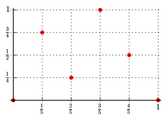
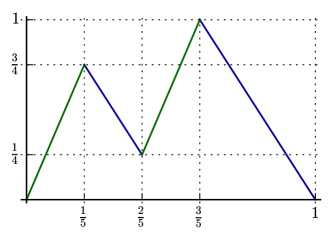
The number of slopes can be taken as a measure of complexity of an extreme function. Functions with only 2 slopes are the easiest to analyze; in fact, the Gomory–Johnson Two Slope Theorem [19] states that any continuous 2-slope function that is minimal valid for $R_{f}(\mathbb{R}/\mathbb{Z})$ is already extreme. Gomory–Johnson in their 2003 paper [21, section 6.2], after discussing the tools available for analyzing minimal functions for the infinite group problem, explain:

[T]heir application to generate facets is still somewhat ad hoc. Also we don’t have general theorems for three or more slope facets analogous to the Gomory–Johnson Two Slope Theorem.

Indeed, functions with 2 or 3 slopes were the focus of much of the literature, as we will discuss in more detail below.

1.3. Computer-based search used in the finite group problem

Gomory’s seminal paper [18, Appendix 5], introducing the group problem and corner polyhedra, listed all extreme functions up to automorphism and homomorphism for the finite group problems of order $q=2,3,\dots,11$. Gomory proved that the set $\Pi_{f}(\frac{1}{q}\mathbb{Z}/\mathbb{Z})$ of minimal functions for $R_{f}(\frac{1}{q}\mathbb{Z}/\mathbb{Z})$ is a polytope, defined by linear inequalities that express subadditivity and certain equations that come from normalization; see Theorem 2.2 below for details. By [18, Theorem 18] and [19, Theorem 2.2], the extreme functions for $R_{f}(\frac{1}{q}\mathbb{Z}/\mathbb{Z})$ are the extreme points of the polytope $\Pi_{f}(\frac{1}{q}\mathbb{Z}/\mathbb{Z})$. Gomory reported that the extreme points were computed, by enumerating simplex bases, using a computer code of Balinski and Wolfe.

During the revival of the interest in the group problem in the 2000s, Evans [16] used her specialized implementation of the double description method (see, e.g., [17]) to enumerate all extreme points of the polytope $\Pi_{f}(\frac{1}{q}\mathbb{Z}/\mathbb{Z})$, thereby obtaining all the extreme functions for the finite group problems of order $q\leq 24$. By exploring the patterns of such functions, some parametric families of 2-slope and 3-slope extreme functions for finite group problems were constructed. Extreme functions from these families were generated by the Matlab code in [16, Appendix B.1] for the finite group problems of order $q\leq 30$. Evans reported that these extreme functions received a large percentage of hits in the so-called shooting experiment [16, Table 13].

Gomory and Johnson [19] showed that the number of extreme functions grows exponentially with $q$. Hence it is impractical to enumerate all extreme functions for $R_{f}(\frac{1}{q}\mathbb{Z},\mathbb{Z})$ when $q$ is large. The shooting experiment was conducted in [22] (more results appeared in [16]) to identify the “important” extreme functions for the finite group problems where the order is at most $30$. This experiment was extended to finite group problems of order up to $90$, and then to problems of order up to $200$ with the so-called “partial shooting” variant in [13]; see also [32]. Extreme functions resulting from the shooting experiments were expected to be important computationally in branch-and-cut (see, e.g., [30, Section 19.6.2] for a summary), though actual computational uses never seem to have materialized. They are mostly gmic functions (up to multiplicative homomorphism and automorphism), along with some other 2-slope and 3-slope extreme functions. The shooting experiment, however, is not suitable for finding functions with many slopes, as those appear to be extremely rare from the viewpoint of shooting, or functions with specific properties for finite group problems. It is not possible to perform the experiment for the infinite group problem either, according to [30, Section 19.6.2.1].

Aráoz, Evans, Gomory and Johnson [1] demonstrated a close relation between the master finite group problem and the master knapsack problem. In particular, the convex hull $P(K_{q-1})$ of solutions to the master knapsack problem of size $q-1$ is a facet of the master finite group problem $R_{f}(\frac{1}{q}\mathbb{Z}/\mathbb{Z})$, where $f=\frac{q-1}{q}$. Thus, extreme functions for $R_{f}(\frac{1}{q}\mathbb{Z}/\mathbb{Z})$ where $f=\frac{q-1}{q}$ are all valid for the knapsack problem $K_{q-1}$. Furthermore, some extreme functions for $R_{f}(\frac{1}{q}\mathbb{Z}/\mathbb{Z})$ may be obtained from facets for $P(K_{qf})$ through a process called tilting (see [1, Theorem 5.2]). Examples of extreme functions derived by tilting a knapsack facet are listed in [1, Table B.2].

A different approach was followed by Richard, Li and Miller [31], who proposed an approximate lifting scheme that converts certain superadditive functions into potentially strong valid inequalities. The superadditive functions that they studied were the $\mathrm{DPL}_{n}$ functions with $4n$ non-negative parameters, and the superadditive $\mathrm{CPL}_{n}$ functions as a special case of $\mathrm{DPL}_{n}$ where $2n$ parameters were fixed to $0$. The parameters that define a superadditive $\mathrm{DPL}_{n}$ function belong to a certain polyhedron $P\Theta_{n}$ (or, in the case of superadditive $\mathrm{CPL}_{n}$ function, to a simpler polyhedron that is a face of $P\Theta_{n}$). Several classes of well-known cutting planes can be generated by converting the $\mathrm{DPL}_{n}$ or $\mathrm{CPL}_{n}$ functions that correspond to the extreme points of $P\Theta_{n}$. However, the functions generated by the approximate lifting scheme are not always extreme. By the lack of any automated extremality tests for a parametric family of functions, the study was restricted to so small $n$ that manual inspection of extremality became possible. The authors investigated the $\mathrm{CPL}_{2}$ functions for the finite group problem in [29] and a special case of $\mathrm{CPL}_{3}$ functions for both finite and infinite group problems in [31], all of which required extensive case analysis for extremality conditions by hand. They found the first parametric family of 4-slope extreme functions for the finite group problem in [31].

1.4. Computer-based search used in the infinite group problem

Computer-based search has also been used in the study of the infinite group problem. One approach focuses on continuous piecewise linear functions $\pi$ with breakpoints in $\tfrac{1}{q}\mathbb{Z}$ for some fixed $q\in\mathbb{Z}_{+}$. (Then, without loss of generality, one can assume that also $f\in\tfrac{1}{q}\mathbb{Z}$ [7, Lemma 2.4].) Gomory and Johnson [19] established a connection between finite and infinite group problems by studying the restriction and interpolation of valid functions. They proved that a continuous piecewise linear function $\pi$ with breakpoints and $f$ in $\frac{1}{q}\mathbb{Z}$ is minimal if and only if its restriction to $\frac{1}{q}\mathbb{Z}$ is minimal for the finite group problem $R_{f}(\tfrac{1}{q}\mathbb{Z}/\mathbb{Z})$. Moreover, if $\pi$ is extreme for $R_{f}(\mathbb{R}/\mathbb{Z})$, then the restriction $\pi|_{\frac{1}{q}\mathbb{Z}}$ is extreme for $R_{f}(\tfrac{1}{q}\mathbb{Z}/\mathbb{Z})$. Therefore all search approaches for the finite group problem, described above in section 1.3, yield candidates for extreme functions for the infinite group problem.

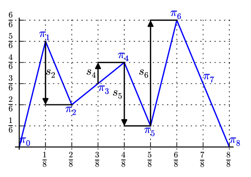
Using this connection with the finite group problem $R_{f}(\tfrac{1}{q}\mathbb{Z}/\mathbb{Z})$ amounts to discretizing the space of functions $\pi$, by discretizing the breakpoints of $\pi$ in $\frac{1}{q}\mathbb{Z}$ for some fixed $q$. A function $\pi$ is then uniquely determined by its values at $\frac{i}{q}$ for $i=0,1,\dots,q$, or by its slope values on the intervals $[\frac{i-1}{q},\frac{i}{q}]$ for $i=1,\dots,q$. We introduce the following notation for use throughout the paper. Denote the function value at $\frac{i}{q}$ by $\pi_{i}$ for $i\in\{0,1,\dots,q\}$, where $\pi_{0}=\pi_{q}=0$. Let $s_{i}$ be real numbers such that $qs_{i}$ are the slope values on $[\frac{i-1}{q},\frac{i}{q}]$ for $i\in\{1,\dots,q\}$. See Figure 2 for an illustration.

Figure 2. The $q\times v$ grid discretization of the space of continuous piecewise linear functions with rational data. Here $q=8$ and $v=6$.

Chen [12] designed an enumerative algorithm to find candidate piecewise linear extreme functions for the infinite group problem using an additional discretization. In addition to fixing $q$, also pick a natural number $v$. Then consider the continuous piecewise linear functions $\pi$ that have $q\times v$ grid discretization: the breakpoints being in $\{0,\frac{1}{q},\dots,\frac{q-1}{q},1\}$ and

1. $\pi_{i}\in\{0,\frac{1}{v},\dots,\frac{v-1}{v},1\}$ for $i\in\{0,\dots,q\}$, or

2. $s_{i}\in\{-1,\dots,\frac{-1}{v},0,\frac{1}{v},\dots,\frac{v-1}{v},1\}$ for $i\in\{1,\dots,q\}$.

In fact, these two natural ways of discretization are easily seen to be equivalent (B.0 in Appendix B). Chen’s algorithm then enumerated every candidate function $\pi$ such that $\pi$ is symmetric, $\pi(0)=0$, $\pi(f)=1$, $\pi(1)=0$, and $\pi$ has the steepest positive and negative slopes at $0$ and $1$ respectively. With $q=10$, $v=9$, almost $500$ functions were found. However, no results were stated regarding the extremality of these candidate functions. In fact, it was not until the breakthrough algorithmic results in [7] that an automated test for extremality for the infinite group problem became possible. Despite the lack of automated test, Chen constructed the first parametric family of 4-slope extreme functions for the infinite group problem in [12].

Gomory–Johnson, in their 2003 paper [21, section 6.3], had written:

[W]e have discussed mainly large facets, families of two-slope facets or three-slope facets. What about much smaller facets? It seems extremely likely that there are much smaller more complex facets all around the big ones.

However, for a brief period, it seemed that with Chen’s functions the peak of complexity had been reached, as no extreme functions with more than 4 slopes were found. In 2009, Dey–Richard in [14] stated as an open question whether there exist extreme functions with more than 4 slopes. The “4-slope conjecture”, asserting that 4 slopes is the maximum for continuous piecewise linear extreme functions, circulated among researchers for a while. The conjecture reflected the hope that, in contrast to the “unstructured and arithmetic” finite group problem, the complexity of the extreme functions of the infinite group problem would be under control. It is unclear how much support the conjecture had at any time; Dey (2016, Personal Communication) remembers that he did not believe in this conjecture.

The 4-slope conjecture had to be revised quickly when new computational tools for testing extremality became available. Basu et al. [7, Theorem 1.5] (see also [10, Theorem 8.5]) showed that in order to test extremality of $\pi$ for $R_{f}(\mathbb{R}/\mathbb{Z})$, one simply needs to test extremality of its restriction to $\frac{1}{4q}\mathbb{Z}$ for $R_{f}(\tfrac{1}{4q}\mathbb{Z}/\mathbb{Z})$. (Later it was shown that restricting to $\frac{1}{3q}$ suffices [10, Theorem 8.6].) This extremality test can be done by computing the rank of a finite-dimensional system of linear equations.

These algorithmic results in [7] enabled Hildebrand to run a new computer-based search, using Matlab programs (2013, unpublished, reported in [9, Table 4]). Like Chen [12], Hildebrand generated functions $\pi$ on the $q\times v$ grid. However, instead of searching exhaustively, he generated the functions randomly. For each candidate function $\pi$, he checked if $\pi|_{\frac{1}{q}\mathbb{Z}}$ is minimal and extreme for $R_{f}(\tfrac{1}{q}\mathbb{Z}/\mathbb{Z})$ (a necessary condition), and finally tested if $\pi|_{\frac{1}{4q}\mathbb{Z}}$ is extreme for $R_{f}(\tfrac{1}{4q}\mathbb{Z}/\mathbb{Z})$ (Basu et al.’s necessary and sufficient condition). In this way, Hildebrand discovered the first 5-slope extreme functions, thus refuting the 4-slope conjecture.

Still it seemed possible that a version of this conjecture might be true; either with $4$ replaced by another small number, or that the 4-slope conjecture holds “generically” (see [8, Open Question 2.16]).

1.5. New search strategies; outline of the paper

In this paper, we develop new search strategies that aim to find extreme functions for the infinite group problem with many different slope values or with special properties. Our goals are markedly different from those of some earlier research surveyed above, in particular from studies using variants of the shooting experiment [22, 13]. We merely wish to settle theoretical questions regarding the structure of extreme functions. We make no claims whatsoever regarding the computational usefulness of the functions that are found by our search.

Our implementation is based on the software [23], which implements an automated extremality test, following the ideas of the proof of [7, Theorem 1.3]. The practical implementation, described in detail in [25, 24], has an empirical running time that does not strongly depend on $q$, and therefore is suitable for functions with extremely large $q$, even though no theoretical worst-case running time bound better than polynomial in $q$ is available.

Like Gomory [18] and Evans [16], and in contrast to Chen’s and Hildebrand’s approaches, our strategies only discretize the breakpoints into $\frac{1}{q}\mathbb{Z}$. This is crucial to be able to reach larger values of $q$, as we explain in Appendix B, where we discuss the complexity of search approaches based on $q\times v$ grid discretization.

1.5.1. Section 2: Vertex filtering search

As a first step of our study, we investigate how far we get by just combining state-of-the-art vertex enumeration software with the automated extremality test provided by the software [23]. We build on state-of-the-art vertex enumeration software, Parma Polyhedra Library (PPL) [4] and lrslib [2, 3]. The vertex filtering search was able to enumerate extreme functions with $q\leq 27$, among which the first 6-slope extreme functions were found, breaking the previous record of $5$ slopes due to Hildebrand (2013, unpublished; reported in [9]). From the results obtained by this search, we observe:

• a diminishing fraction of vertices of $\Pi_{f}(\frac{1}{q}\mathbb{Z}/\mathbb{Z})$ that correspond to extreme functions for $R_{f}(\mathbb{R}/\mathbb{Z})$;

• an exponential growth of time spent on vertex enumeration;

when $q$ increases.

1.5.2. Section 3: Search using MIP

These factors suggest that one needs to consider other search strategies to reach larger $q$. We investigate search strategies that, for the first time, are guided directly by the subtle structure of minimal functions that were exposed by the proof of the algorithmic extremality test in [7], rather than using the extremality test merely as a black box.

To this end, we review the notions of the two-dimensional polyhedral complex $\Delta\mathcal{P}$ and of additive faces in section 3.1. Identifying the additive faces of $\Delta\mathcal{P}$ is a crucial step in the algorithmic extremality test [7]. By means of Gomory–Johnson’s celebrated Interval Lemma, additive faces give rise to “affine-imposing” intervals (in the terminology of [7]). This reduces the infinite-dimensional test to a finite-dimensional one. The combinatorics of the additive faces of the complex $\Delta\mathcal{P}$ has a central role in our new approaches.

In the remainder of section 3 we describe how the search based on the combinatorics of the additive faces can be implemented using standard MIP modeling techniques and running a commercial MIP solver. This is easy to implement and easy to tailor to a search for extreme functions with particular properties. However it is limited because floating-point implementations are not a good match for finding functions of high arithmetic complexity, and because MIP solvers are generally not the best tool for performing an exhaustive search.

1.5.3. Section 4: Backtracking search

To address the shortcomings of the MIP approach, we have developed a specialized backtracking search algorithm, which we describe in section 4. Like the MIP approach, it is based on the combinatorics of the additive faces. It works best when combined with the vertex filtering search described in section 2. This combined search algorithm looks for extreme functions by backtracking on the additive faces of $\Delta\mathcal{P}$ in a first step and vertex enumeration in a second step. The synergy and balance between these two steps to obtain the best computational performance is discussed in section 4.7. Using the combined search algorithm, we discover new extreme functions with up to 7 slopes.

1.5.4. Section 5: Targeted search with patterns

In the library of functions found by the above algorithms, we observe some special combinatorial patterns on their two-dimensional polyhedral complexes $\Delta\mathcal{P}$. In section 5, we describe how we use these patterns to make a targeted search for functions with a very large number of slopes, which discovers piecewise linear extreme functions with up to 28 slopes.

1.6. Summary of new results

Theorem 1.1.

There exist continuous piecewise linear extreme functions with $2$, $3$, $4$, $5$, $6$, $7$, $8$, $10$, $12$, $14$, $16$, $18$, $20$, $22$, $24$, $26$, and $28$ slopes.

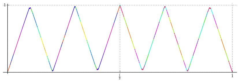
Figure 3 shows one 28-slope extreme function found by our code, with $q=778$, out of reach for any previous study. We remark that Basu et al. [6] have improved Theorem 1.1 by constructing a family of extreme functions with an arbitrary prescribed number of slopes.

Figure 3. A 28-slope extreme function kzh_28_slope_1 found by our search code. Each color in the plotting corresponds to a different slope value.

Our computer-based search also can be tailored to find extreme functions with certain properties. In particular, several open questions are resolved by such newly discovered extreme functions. Let $m\geq 3$ be a positive integer. [10, Theorem 8.6] states that $\pi$ is extreme for $R_{f}(\mathbb{R}/\mathbb{Z})$ if and only if the restriction $\pi|_{\frac{1}{mq}\mathbb{Z}}$ is extreme for the finite group problem $R_{f}(\tfrac{1}{mq}\mathbb{Z}/\mathbb{Z})$. Our search found a function (see Figure 4) that is not extreme for $R_{f}(\mathbb{R}/\mathbb{Z})$, but whose restriction to $\frac{1}{2q}\mathbb{Z}$ is extreme for $R_{f}(\frac{1}{2q}\mathbb{Z}/\mathbb{Z})$.

Figure 4. The example kzh_2q_example_1, showing that an oversampling factor of $m=3$ in [10, Theorem 8.6] is best possible.

This proves the following result, thereby answering the Open Question 8.7 in [8].

Proposition 1.1.

The hypothesis $m\geq 3$ in [10, Theorem 8.6] is best possible. The theorem does not hold for $m=2$.

The search also found piecewise linear extreme functions of $R_{f}(\mathbb{R}/\mathbb{Z})$ to answer the Open Question 2.16 in [8], which we mentioned in section 1.4.

1.7. Available software

We have made all of the discovered functions mentioned in this paper available as part of the Electronic Compendium [35]. The reader is invited to investigate the functions using our software [23]. The articles [25, 24] describe the software in detail. The computer-based search code will be released shortly as part of a new version of the software [23].

2. Restriction to $q$ grid – Vertex filtering search

Recall that we are looking for continuous piecewise linear functions $\pi\colon\mathbb{R}\rightarrow\mathbb{R}_{+}$ with breakpoints in $\tfrac{1}{q}\mathbb{Z}$ that are extreme for the single-row Gomory–Johnson infinite group problem. The construction of parametric families of extreme functions (a focus of many previous studies), extreme functions with irrational breakpoints (for example, the function bhk_irrational in [7]), and non–piecewise linear extreme functions such as bccz_counterexample [5] are beyond the scope of this paper.

2.1. Restriction to grid

Our approach is based on the discretization of the breakpoints of $\pi$. More precisely, we only focus on the functions $\pi$ with rational breakpoints in $\tfrac{1}{q}\mathbb{Z}$ for some $q\in\mathbb{N}$. Suppose without loss of generality [7, Lemma 2.4] that $f\in\tfrac{1}{q}\mathbb{Z}$. Under such hypotheses, $\pi$ is uniquely determined by its values at points in $\tfrac{1}{q}\mathbb{Z}$. We say that $\pi$ is the (continuous) interpolation of $\pi|_{\frac{1}{q}\mathbb{Z}}$, while $\pi|_{\frac{1}{q}\mathbb{Z}}$ is the restriction of $\pi$ to the grid $\tfrac{1}{q}\mathbb{Z}$. footnote 3 in section 1 illustrates the interpolation and restriction of a gj_2_slope function with $q=5$.

Gomory and Johnson proved the following relations between $\pi$ and $\pi|_{\frac{1}{q}\mathbb{Z}}$:

Theorem 2.1 ([19]; see also [10, Theorem 8.3]).

Let $\pi$ be a continuous piecewise linear function with breakpoints in $\tfrac{1}{q}\mathbb{Z}$ for some $q\in\mathbb{Z}_{+}$ and let $f\in\tfrac{1}{q}\mathbb{Z}$. Then the following hold:

1. $\pi$ is minimal for $R_{f}(\mathbb{R}/\mathbb{Z})$ if and only if $\pi|_{\frac{1}{q}\mathbb{Z}}$ is minimal for $R_{f}(\tfrac{1}{q}\mathbb{Z}/\mathbb{Z})$.

2. If $\pi$ is extreme for $R_{f}(\mathbb{R}/\mathbb{Z})$, then $\pi|_{\frac{1}{q}\mathbb{Z}}$ is extreme for $R_{f}(\tfrac{1}{q}\mathbb{Z}/\mathbb{Z})$.

Hence the interpolations of those $\pi|_{\frac{1}{q}\mathbb{Z}}$ that are extreme for $R_{f}(\tfrac{1}{q}\mathbb{Z}/\mathbb{Z})$ are the only possible candidates of continuous piecewise linear extreme functions with breakpoints in $\frac{1}{q}\mathbb{Z}$ for $R_{f}(\mathbb{R}/\mathbb{Z})$. Extreme functions are clearly minimal functions; the latter have a characterization given by a theorem by Gomory and Johnson. In the case of the finite group problem $R_{f}(\tfrac{1}{q}\mathbb{Z}/\mathbb{Z})$, it can be stated as follows.

Theorem 2.2 ([19]; see also [9, Theorem 2.6]).

Let $\pi$ and $f$ be as above. $\pi|_{\frac{1}{q}\mathbb{Z}}$ is minimal for $R_{f}(\tfrac{1}{q}\mathbb{Z}/\mathbb{Z})$ if and only if

1. $\pi_{0}=0$,

2. $\pi|_{\frac{1}{q}\mathbb{Z}}$ is subadditive: $\pi_{(x+y)\bmod q}\leq\pi_{x}+\pi_{y}$ for $x,y\in\mathbb{Z}$,

3. $\pi|_{\frac{1}{q}\mathbb{Z}}$ is symmetric: $\pi_{x}+\pi_{qf-x}=1$ for $x\in\mathbb{Z}$,

where $\pi_{i}=\pi(\frac{i}{q})$ for $i\in\mathbb{Z}$.

Since $\pi\colon\mathbb{R}/\mathbb{Z}\to\mathbb{R}$ is periodic modulo $1$, a minimal function $\pi|_{\frac{1}{q}\mathbb{Z}}$ for the finite group problem is specified by its values $(\pi_{0},\pi_{1},\dots,\pi_{q-1})$ on the grid points $\tfrac{1}{q}\mathbb{Z}\cap[0,1)$. The following statement immediately follows from the observation that the above conditions are all linear constraints.

Proposition 2.2 ([19, Theorem 2.2]).

The set $\Pi_{f}(\frac{1}{q}\mathbb{Z}/\mathbb{Z})$ of minimal functions for $R_{f}(\tfrac{1}{q}\mathbb{Z}/\mathbb{Z})$ is a convex polytope. Furthermore, extreme functions for $R_{f}(\tfrac{1}{q}\mathbb{Z}/\mathbb{Z})$ are the extreme points (i.e., vertices) of this polytope.

By Theorem 2.1 and 2.2, all continuous piecewise linear extreme functions for $R_{f}(\mathbb{R}/\mathbb{Z})$ with breakpoints in $\frac{1}{q}\mathbb{Z}$ can be found by interpolating the vertices of the polytope $\Pi_{f}(\tfrac{1}{q}\mathbb{Z}/\mathbb{Z})$. However, in general, extremality of $\pi|_{\frac{1}{q}\mathbb{Z}}$ for $R_{f}(\frac{1}{q}\mathbb{Z}/\mathbb{Z})$ does not imply extremality of $\pi$ for $R_{f}(\mathbb{R}/\mathbb{Z})$. This makes further filtering necessary, which we explain below.

2.2. Preprocessing

We begin with a remark on the minimal H-representation of $\Pi_{f}(\frac{1}{q}\mathbb{Z}/\mathbb{Z})$. The H-representation of the polytope $\Pi_{f}(\frac{1}{q}\mathbb{Z}/\mathbb{Z})$ defined by Theorem 2.2 has asymptotically $\frac{1}{2}q^{2}$ constraints, many of which are redundant. Indeed, [33, Corollary 2.7] gives a minimal representation of $\Pi_{f}(\frac{1}{q}\mathbb{Z}/\mathbb{Z})$ that only has asymptotically $\frac{1}{6}q^{2}$ constraints, mainly by replacing the subadditivity constraints (2) of Theorem 2.2:

$$\pi_{i}+\pi_{j}\geq\pi_{(i+j)\bmod q}\text{ for }0\leq i\leq j<q$$

with the triple system:

$$\pi_{i}+\pi_{j}+\pi_{k}\geq 1\text{ for }0\leq i\leq j\leq k<q,\;i+j+k=qf\pmod{q}.$$

A minimal H-representation is of interest for vertex enumeration, because having many redundant inequalities may greatly slow down the vertex enumeration process. Although a minimal H-representation is known for the polytope $\Pi_{f}(\frac{1}{q}\mathbb{Z}/\mathbb{Z})$, the search strategies described in later sections of the present paper also need to deal with other polytopes whose minimal H-representations are not known. For this purpose, computational preprocessing is used to remove the redundant inequalities from the H-representation of a polytope before enumerating its vertices. Namely, we apply the preprocessing program redund provided by lrslib (version 5.0), which removes redundant inequalities using Linear Programming. The third columns of Tables 1 and Table 2 show the number of inequalities in the H-representation of the polytope $\Pi_{f}(\frac{1}{q}\mathbb{Z}/\mathbb{Z})$ for $f=\frac{1}{q}$ before and after preprocessing, respectively. The number after preprocessing is roughly $\frac{1}{6}q^{2}$, which is consistent with [33, Corollary 2.7].

2.3. Performance of various vertex enumeration codes

Various software packages are available for computing the vertices of a polytope given by an H-representation. We considered the following popular packages.

• cddlib (version 094g), a well-known implementation of the double description method [17].

• Parma Polyhedra Library (version 1.1). PPL is a C++ library for the manipulation and computation of rational convex polyhedra [4]. Like cddlib, polyhedral computations in PPL are based on the double description method.

  An extensive computational study [4, section 4] showed that the double description method implementation in PPL has a better performance (on the vertex/facet enumeration problem) compared with cddlib and with other polyhedra libraries that are popular in PPL’s primary application domain, New Polka and PolyLib.

• Porta (version 1.4.1), based on the Fourier–Motzkin elimination method.

• lrslib (version 5.0), a C implementation of the lexicographic reverse search algorithm for vertex enumeration and convex hull problems [2, 3]. This algorithm uses little memory space during the computation; vertices are generated as a stream and are not stored in memory, which makes it suitable for vertex enumeration problems for polytopes with a large number of vertices.

  The computational study [4, Table 2] showed that lrslib outperforms PPL for large problems, whereas PPL outperforms lrslib for easy problems [4, Table 1].

Based on the study [4], we expected PPL to be the best choice for low dimensions and lrslib to be the best choice for high dimensions. We decided to verify this using a computational study for our polytopes $\Pi_{f}(\tfrac{1}{q}\mathbb{Z}/\mathbb{Z})$ given in 2.2 for various values of $q$ and $f=\tfrac{1}{q}$, recording the running times for vertex enumeration.

In addition to the four packages listed above, we also included the following package in our experiments, which was developed very recently and had not been investigated in a major computational study.

• PANDA (version 2015-02-24) based on the parallel adjacency decomposition algorithm [28].

At the time of the revision of the present paper, we also became aware of the high performance vertex enumeration code in the following package.

• Normaliz (version 3.1.1), a software tool for the computation of Hilbert bases and enumerative data of rational cones and affine monoids. Its vertex enumeration code is based on the Fourier–Motzkin elimination method and the pyramid decomposition described in [11].

We used PPL via its Cython-based library interface within the SageMath [34] computer algebra system. The other systems were tested using their command-line executables because no library interfaces were available for them in SageMath. Hence in very low dimension, there is a slight bias in favor of PPL due to the overhead in using the other systems via executables and file passing. All systems were tested using exact computation modes and using a single thread.

Tables 1 and 2 report for each test the size of the polytope and the running times measured in CPU seconds, without and with preprocessing, respectively. The preprocessing in Table 2 consists of removing redundant inequalities from the H-representation using the command redund provided by lrslib. We also measured the computational overhead of interfacing to redund in Python, which exceeds the actual redund running times. Comparing Table 1 and Table 2 shows that for dimension at most $6$, it is best to just run PPL on the original inequalities without preprocessing. For dimensions at least $7$, Normaliz is the clear winner. The total time for preprocessing pays off when the dimension of the polytope is at least $10$ for Normaliz, or is at least $8$ for the other systems. For dimension at least $13$, Normaliz is faster than the second-best code, lrslib, by more than an order of magnitude. Normaliz is also the least dependent on preprocessing.

For the computational experiments in the remainder of this paper, we used a combination of PPL (for low dimensions) and lrslib (for high dimensions), using preprocessing when the dimension is at least $8$. We did not use Normaliz, as we only became aware of its high performance code for vertex enumeration at the time of revision of the present paper.

2.4. Filtering

As mentioned earlier, extremality of $\pi|_{\frac{1}{q}\mathbb{Z}}$ for $R_{f}(\frac{1}{q}\mathbb{Z}/\mathbb{Z})$ does not always imply extremality of $\pi$ for $R_{f}(\mathbb{R}/\mathbb{Z})$. We call the interpolation $\pi$ of a vertex $\pi|_{\frac{1}{q}\mathbb{Z}}$ of the polytope $\Pi_{f}(\tfrac{1}{q}\mathbb{Z}/\mathbb{Z})$ a vertex-function. Once the vertices of $\Pi_{f}(\frac{1}{q}\mathbb{Z}/\mathbb{Z})$ are enumerated, we can use the automated extremality test implemented in the software [23, 25, 24] to filter out those $\pi|_{\frac{1}{q}\mathbb{Z}}$ whose interpolations are not extreme for $R_{f}(\mathbb{R}/\mathbb{Z})$. We will discuss in section 3.1 the two-dimensional polyhedral complex $\Delta\mathcal{P}$ and the notion of covered intervals that make this automated extremality test possible.

Remark 2.2.

Given that $\pi|_{\frac{1}{q}\mathbb{Z}}$ is a vertex of $\Pi_{f}(\frac{1}{q}\mathbb{Z}/\mathbb{Z})$, the extremality test of $\pi$ for $R_{f}(\mathbb{R}/\mathbb{Z})$ reduces to testing whether all intervals are covered, according to Theorem 3.1. This can be determined using the function generate_uncovered_intervals of [23].

We now summarize the above ideas in the following algorithm, which is referred to as “vertex filtering mode” in our code. The implementation uses Parma Polyhedra Library and lrslib as described in section A.1.

1. Consider the restriction of $\pi$ to the grid $\tfrac{1}{q}\mathbb{Z}$.

Define $\pi_{0},\pi_{1},\dots,\pi_{q}$ as variables, where $\pi_{i}=\pi(\frac{i}{q})$.

Construct the polytope $\Pi_{f}(\tfrac{1}{q}\mathbb{Z}/\mathbb{Z})$ of minimal functions for $R_{f}(\tfrac{1}{q}\mathbb{Z}/\mathbb{Z})$, defined by Theorem 2.2. (3) Enumerate the vertices $\pi|_{\frac{1}{q}\mathbb{Z}}$ of this polytope. (4) For every vertex $\pi|_{\frac{1}{q}\mathbb{Z}}$, do: (a) Interpolate to get $\pi$, a minimal valid function for $R_{f}(\mathbb{R}/\mathbb{Z})$. (b) If the intervals $[\frac{i}{q},\frac{i+1}{q}]$ for $i=0,1,\dots,q-1$ are all covered, then $\pi$ is extreme for $R_{f}(\mathbb{R}/\mathbb{Z})$. Output function $\pi$.

Algorithm 1 vertex filtering mode

2.5. Performance of the vertex filtering search

Our search code is implemented in SageMath [34], an open-source mathematics software system that uses Python and Cython as its primary programming languages and interfaces with various existing packages.

Our vertex filtering search code uses the strategies described in section 2.3 to decide whether preprocessing is needed and which software to use for vertex enumeration. We test its performance for $q=10,11,\dots,27$ and $f=\frac{x}{q}$ for $x=1,2,\dots,\lfloor\frac{q}{2}\rfloor$.

Figure 5. Vertex enumeration time (not including checking extremality of vertex-functions), mean extremality checking time for a vertex-function, and percentage of extreme functions

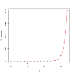
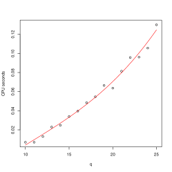
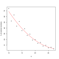
Observe that as $q$ increases, the dimension and the number of vertices of the polytope increase. In particular, it results in an exponential growth of running time for vertex enumeration (cf. Figure 5–left). In addition to vertex enumeration, the vertex filtering search has to run extremality tests for the vertex-functions once they are found, which consumes non-negligible extra time (cf. Figure 5–middle). Furthermore, Figure 5–right illustrates a decrease in the percentage of extreme functions to vertex-functions. It suggests that when $q$ is large, vertex filtering search does enumeration in high dimension and throws away many non-extreme functions. Therefore, it is not surprising that the vertex filtering search is only suitable for small $q$ ($q\leq 27$).

2.6. Results and discussion

Despite its limitations, vertex filtering search finds up to 6-slope extreme functions with $q\leq 27$, breaking the previous record of 5 slopes due to Hildebrand (2013, unpublished).

The extreme functions obtained from the vertex filtering search with breakpoints in $\frac{1}{q}\mathbb{Z}/\mathbb{Z}$ ($q\leq 27$) for the infinite and finite group problems are plotted in Figure 6, using blue and red dots. They are placed from left to right according to the value $q$ and the number of slopes. The log-scale $y$-axis refers to the arithmetic complexity of the extreme functions, which we define as follows.

Definition 2.2.

The arithmetic complexity of a function $\pi\colon\frac{1}{q}\mathbb{Z}/\mathbb{Z}\to[0,1]$ (or of a continuous piecewise linear function $\pi\colon\mathbb{R}/\mathbb{Z}\to[0,1]$ with breakpoints in $\tfrac{1}{q}\mathbb{Z}$) is defined as the least common denominator of the values $\pi_{i}=\pi(\frac{i}{q})$ for $i\in\{0,\dots,q\}$.

For example, it is easy to see that the gmic function with $f\in\tfrac{1}{q}\mathbb{Z}$ has an arithmetic complexity of $O(q^{2})$.

We observe from Figure 6 an empirical exponential growth of the arithmetic complexity as $q$ increases. This suggests that huge values of $v$ would be needed in a search based on the $q\times v$ grid discretization, like Chen’s and Hildebrand’s described in section 1.4), in order to make them exhaustive. This renders this approach unsuitable for large $q$.

In the following, we give an upper bound on the arithmetic complexity of an extreme function in terms of $q$. We will refer to this bound in the following sections. Let $\pi$ be an extreme function for $R_{f}(\frac{1}{q}\mathbb{Z}/\mathbb{Z})$. 2.2 states that $(\pi_{0},\pi_{1},\dots,\pi_{q-1})$ is a vertex of the polytope $\Pi_{f}(\frac{1}{q}\mathbb{Z}/\mathbb{Z})$ defined in Theorem 2.2. By introducing slack variables, the constraint system of $\Pi_{f}(\frac{1}{q}\mathbb{Z}/\mathbb{Z})$ can be written in the standard form using matrix notation as $A{\mathchoice{\mbox{\boldmath$\displaystyle\bf x$}}{\mbox{\boldmath$\textstyle\bf x$}}{\mbox{\boldmath$\scriptstyle\bf x$}}{\mbox{\boldmath$\scriptscriptstyle\bf x$}}}={\mathchoice{\mbox{\boldmath$\displaystyle\bf b$}}{\mbox{\boldmath$\textstyle\bf b$}}{\mbox{\boldmath$\scriptstyle\bf b$}}{\mbox{\boldmath$\scriptscriptstyle\bf b$}}},{\mathchoice{\mbox{\boldmath$\displaystyle\bf x$}}{\mbox{\boldmath$\textstyle\bf x$}}{\mbox{\boldmath$\scriptstyle\bf x$}}{\mbox{\boldmath$\scriptscriptstyle\bf x$}}}\geq\mathchoice{\mbox{\boldmath$\displaystyle\bf 0$}}{\mbox{\boldmath$\textstyle\bf 0$}}{\mbox{\boldmath$\scriptstyle\bf 0$}}{\mbox{\boldmath$\scriptscriptstyle\bf 0$}}$, where $A$ and $\textstyle\bf b$ have all integer entries. Then by Cramer’s rule, the denominators of $\{\pi_{i}\}_{i=0,1,\dots,q-1}$ come from the inverse of simplex basis matrices. The next lemma investigates the determinants of simplex basis matrices of $A$. The proof of this lemma appears in Appendix B.

Lemma 2.2.

Let $q\in\mathbb{Z}_{+}$ and $f\in\frac{1}{q}\mathbb{Z}$, $0<f<1$. Let $A{\mathchoice{\mbox{\boldmath$\displaystyle\bf x$}}{\mbox{\boldmath$\textstyle\bf x$}}{\mbox{\boldmath$\scriptstyle\bf x$}}{\mbox{\boldmath$\scriptscriptstyle\bf x$}}}={\mathchoice{\mbox{\boldmath$\displaystyle\bf b$}}{\mbox{\boldmath$\textstyle\bf b$}}{\mbox{\boldmath$\scriptstyle\bf b$}}{\mbox{\boldmath$\scriptscriptstyle\bf b$}}}$, ${\mathchoice{\mbox{\boldmath$\displaystyle\bf x$}}{\mbox{\boldmath$\textstyle\bf x$}}{\mbox{\boldmath$\scriptstyle\bf x$}}{\mbox{\boldmath$\scriptscriptstyle\bf x$}}}\geq\mathchoice{\mbox{\boldmath$\displaystyle\bf 0$}}{\mbox{\boldmath$\textstyle\bf 0$}}{\mbox{\boldmath$\scriptstyle\bf 0$}}{\mbox{\boldmath$\scriptscriptstyle\bf 0$}}$ be the constraint system of Theorem 2.2 written in the standard form. Let $B$ be a basis matrix of $A$. Then $\mathopen{|}\det B|\leq 10^{{q}/{4}}$.

Given $q\in\mathbb{Z}_{+}$, let $d_{\text{ver}}$ and $d_{\text{ext}}$ denote the maximum arithmetic complexities of any extreme function $\pi$ for $R_{f}(\frac{1}{q}\mathbb{Z}/\mathbb{Z})$ and of any extreme function $\pi$ for $R_{f}(\mathbb{R}/\mathbb{Z})$ with breakpoints in $\frac{1}{q}\mathbb{Z}$, respectively. By Theorem 2.1 and 2.2, it is clear that the number $d_{\text{ext}}$ is well-defined and $d_{\text{ext}}\leq d_{\text{ver}}$. Since the entries of the right-hand side $\textstyle\bf b$ of $A{\mathchoice{\mbox{\boldmath$\displaystyle\bf x$}}{\mbox{\boldmath$\textstyle\bf x$}}{\mbox{\boldmath$\scriptstyle\bf x$}}{\mbox{\boldmath$\scriptscriptstyle\bf x$}}}={\mathchoice{\mbox{\boldmath$\displaystyle\bf b$}}{\mbox{\boldmath$\textstyle\bf b$}}{\mbox{\boldmath$\scriptstyle\bf b$}}{\mbox{\boldmath$\scriptscriptstyle\bf b$}}}$ are integers, we have that

$$d_{\text{ext}}\leq d_{\text{ver}}\leq d_{\text{bas}}:=\max\{\,\mathopen{|}\det B|:B\text{ is a basis matrix of }A\,\}\leq 10^{q/4}.$$

We state this upper bound on $d_{\text{ver}}$ and on $d_{\text{ext}}$ as a corollary.

Corollary 2.2.

Let $\pi$ be an extreme function for $R_{f}(\mathbb{R}/\mathbb{Z})$ with breakpoints in $\frac{1}{q}\mathbb{Z}$ (or an extreme function for $R_{f}(\frac{1}{q}\mathbb{Z}/\mathbb{Z})$). Then the arithmetic complexity of $\pi$ (i.e., the least common denominator of $(\pi_{0},\pi_{1},\dots,\pi_{q})$) is at most $10^{q/4}$.

We do not have a matching lower bound for $d_{\text{ext}}$; however, B.0 in Appendix B offers an exponential lower bound on $d_{\text{bas}}$ when an arithmetic condition on $q$ and $f$ is satisfied.

Table 1. Efficiency of various vertex enumeration codes without preprocessing

				Running time (s)
$q$	dimension	inequalities	vertices	PPL	Porta	cddlib	lrslib	Panda	Normaliz
05	01	021	00002	0.001	0.018	0.009	0.008	0.026	0.003
07	02	036	00004	0.001	0.012	0.011	0.005	0.026	0.004
09	03	055	00007	0.002	0.016	0.018	0.004	0.065	0.005
11	04	078	00018	0.003	0.016	0.031	0.009	23.000	0.007
13	05	105	00040	0.007	0.018	0.11	0.021	4604.000	0.011
15	06	136	00068	0.017	0.037	0.21	0.14		0.017
17	07	171	00251	0.14	0.20	1.200	0.71		0.047
19	08	210	00726	0.91	1.600	5.000	2.300		0.16
21	09	253	01661	6.600	13.000	24.000	13.000		0.67
23	10	300	07188	166.000	558.000	785.000	74.000		4.900
25	11	351	23214	1854.000	10048.000	12129.000	471.000		21.000
26	12	378	54010				2167.000		62.000
27	12	406	68216						89.000
28	13	435	195229						326.000
29	13	465	317145						644.000
30	14	496	576696						1693.000
31	14	528	1216944						3411.000

Table 2. Efficiency of various vertex enumeration codes with preprocessing

				Running time (s)
$q$	dim	ineqs	vertices	PPL	Porta	cddlib	lrslib	Panda	Normaliz	redund	overhead
05	01	007	2	0.003	0.009	0.006	0.010	0.019	0.003	0.006	0.040
07	02	010	4	0.001	0.010	0.009	0.007	0.015	0.003	0.006	0.029
09	03	014	7	0.001	0.008	0.009	0.008	0.021	0.004	0.009	0.010
11	04	020	18	0.002	0.008	0.015	0.010	0.017	0.006	0.012	0.049
13	05	027	40	0.003	0.007	0.021	0.012	0.039	0.009	0.022	0.050
15	06	035	68	0.004	0.012	0.032	0.025	0.040	0.012	0.041	0.14
17	07	045	251	0.016	0.030	0.22	0.10	0.16	0.029	0.041	0.21
19	08	056	726	0.061	0.087	0.34	0.48	0.44	0.085	0.16	0.40
21	09	068	1661	0.25	0.25	1.100	2.500	3.100	0.22	0.25	0.72
23	10	082	7188	4.000	4.100	8.000	15.000	9.000	1.300	0.46	1.100
25	11	097	23214	69.000	43.000	31.000	94.000	15 h00	6.000	0.75	1.800
26	12	115	54010	511.000	350.000	692.000	594.000		21.000	0.95	2.600
27	12	113	68216	433.000	493.000	672.000	543.000		23.000	1.000	3.000
28	13	133	195229	8399.000	5796.000	9550.000	3617.000		102.000	1.600	4.000
29	13	131	317145	18361.000	11341.000		3366.000		158.000	1.900	4.900
30	14	152	576696	$>1$ d.000	66747.000		22743.000		488.000	2.500	6.100
31	14	150	1216944	$>3$ d.000	$>2$ d.000		20407.000		734.000	2.800	7.800

Table 3. The arithmetic complexity of the search based on $q\times v$ grid discretization. $d_{\text{ext}}$ and $d_{\text{ver}}$ are the empirical values of $v$ for infinite and finite group problems, and $\mathopen{|}\det B|$ is the estimated value from B.0.

$q$	10	11	12	13	14	15	16	17	18	19	20	21	22	23	24	25	26	27
$d_{\text{ext}}$	21	30	35	48	51	64	63	120	91	168	165	208	255	348	289	504	459	800
$d_{\text{ver}}$	21	30	35	48	51	70	65	138	95	210	165	250	315	570	425	768	651	1120
$\mathopen{|}\det B|$		32		64		128		256		512		1024		2048		4096		8192

Figure 6. Arithmetic complexity and number of slopes depending on $q$. Extreme functions $\pi$ with breakpoints in $\frac{1}{q}\mathbb{Z}/\mathbb{Z}$ for $R_{f}(\mathbb{R}/\mathbb{Z})$ and for $R_{f}(\frac{1}{q}\mathbb{Z}/\mathbb{Z})$ are plotted in dark blue and bright red, respectively. The $x$-axis refers to the value $q$. Within the same value $q$, extreme functions $\pi$ are placed in ascending order by their number of slopes, from left ($2$ slopes) to right. The log-scale $y$-axis refers to the arithmetic complexity of the extreme functions $\pi$, i.e., the least common denominator of $\{\pi_{0},\pi_{1},\dots,\pi_{q-1}\}$, showing the complexity of an exhaustive search based on $q\times v$ grid discretization.

3. MIP approach

In this section we present a new approach for computer-based search for extreme functions. It uses standard mixed integer linear programming (MIP) modeling techniques to obtain a MIP that mimics the algorithmic extremality test due to Basu et al. [7].

3.1. The two-dimensional polyhedral complex $\Delta\mathcal{P}$

We first review the notion of a two-dimensional polyhedral complex, which serves as a tool for studying additivity relations and covered (affine imposing) intervals of piecewise linear functions. We follow [9, Section 3], but define the notions in our case where the function $\pi$ is continuous, piecewise linear and has all its breakpoints in $\tfrac{1}{q}\mathbb{Z}$. This matches the setting of [7]. Since a minimal function is periodic modulo 1, we can restrict the study to the domain $[0,1]$ only. We define the evenly spaced one-dimensional polyhedral complex $\mathcal{P}_{\frac{1}{q}\mathbb{Z}}$ to be the collection of singletons and elementary closed intervals on the grid $\tfrac{1}{q}\mathbb{Z}$ by

$$\mathcal{P}_{\frac{1}{q}\mathbb{Z}}:=\left\{\,\emptyset,\{\tfrac{0}{q}\},\{\tfrac{1}{q}\},\dots,\{\tfrac{q}{q}\},[\tfrac{0}{q},\tfrac{1}{q}],[\tfrac{1}{q},\tfrac{2}{q}],\dots,[\tfrac{q-1}{q},1]\,\right\}.$$

For any $I,J,K\in\mathcal{P}_{\frac{1}{q}\mathbb{Z}}$, let

$$F(I,J,K):=\left\{\,(x,y)\in I\times J:x\oplus y\in K\,\right\}\subseteq[0,1]\times[0,1],$$

where $x\oplus y=(x+y)\bmod 1$. Then the set

$$\Delta\mathcal{P}_{\frac{1}{q}\mathbb{Z}}:=\left\{\,F(I,J,K):I,J,K\in\mathcal{P}_{\frac{1}{q}\mathbb{Z}}\,\right\}$$

is a two-dimensional polyhedral complex. It is the collection of the elementary upper or lower triangles on the grid $\tfrac{1}{q}\mathbb{Z}\times\tfrac{1}{q}\mathbb{Z}$ with the vertices (zero-dimensional faces) and edges (one-dimensional faces) that arise as intersections of these triangles (two-dimensional faces). See Figure 7 for an illustration.

Define the subadditivity slack $\Delta\pi\colon[0,1]\times[0,1]\rightarrow\mathbb{R}$ of $\pi$ by

$$\Delta\pi(x,y):=\pi(x)+\pi(y)-\pi(x\oplus y)$$

for $x,y\in[0,1]$. Note that $\Delta\pi$ is non-negative if $\pi$ is minimal, since minimality implies subadditivity. A face $F$ of the two-dimensional polyhedral complex $\Delta\mathcal{P}_{\frac{1}{q}\mathbb{Z}}$ is said to be additive if $\Delta\pi=0$ on $F$. Together the additive faces form the additivity domain of the function $\pi$. Since $\pi$ is linear on the intervals of $\mathcal{P}_{\frac{1}{q}\mathbb{Z}}$, the function $\Delta\pi$ is linear on the faces of the two-dimensional complex $\Delta\mathcal{P}_{\frac{1}{q}\mathbb{Z}}$. Hence, the condition above is equivalent to $\Delta\pi=0$ on the set of vertices of $F$.

In the diagrams of the polyhedral complex $\Delta\mathcal{P}_{\frac{1}{q}\mathbb{Z}}$ such as Figure 7, we indicate additive faces by various colors. Isolated additive points and additive edges are always drawn in green; two-dimensional additive faces (triangles) are painted in various colors, the significance of which we shall explain below. If a triangle is white, this means that strict subadditivity holds in the interior of this face. We will often refer to the diagram of the additive faces as the painting of $\pi$ on the complex $\Delta\mathcal{P}_{\frac{1}{q}\mathbb{Z}}$.

An additive face implies, among other things, the important covering (affine imposing in the terminology of [7]) property that we outline here. We refer the reader to [9, Section 4] for details on the Interval Lemma and its generalizations.

Define the projections $p_{1},p_{2},p_{3}\colon[0,1]\times[0,1]\to[0,1]$ by

$$p_{1}(x,y)=x,\quad p_{2}(x,y)=y,\quad p_{3}(x,y)=x\oplus y.$$

Figure 7. Diagram of a minimal valid function (graphs on the top and the left) on the grid $\frac{1}{10}\mathbb{Z}$ and the corresponding painting on the two-dimensional polyhedral complex $\Delta\mathcal{P}_{\frac{1}{10}\mathbb{Z}}$ (gray solid lines), as plotted by the command plot_2d_diagram($\pi$, colorful=True), where $\pi$ = not_extreme_1(). Faces of $\Delta\mathcal{P}_{\frac{1}{10}\mathbb{Z}}$ on which $\Delta\pi=0$, i.e., additivity holds, are shaded in colors that correspond to the 4 connected components of this function. The heavy diagonal green lines $x+y=f$ and $x+y=1+f$ correspond to the symmetry condition. At the borders, the projections $p_{i}(F)$ of two-dimensional additive faces are shown as gray shadows: $p_{1}(F)$ at the top border, $p_{2}(F)$ at the left border, $p_{3}(F)$ at the bottom and the right borders.

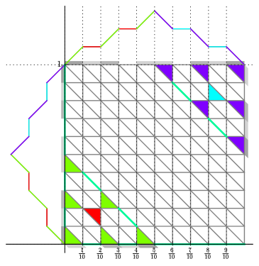
Let $F$ be a two-dimensional additive face of $\Delta\mathcal{P}_{\frac{1}{q}\mathbb{Z}}$ (i.e., $F$ is an elementary upper or lower triangle in the two-dimensional polyhedral complex such that $\Delta\pi=0$ on $F$). By the convex additivity domain lemma for continuous functions [9, Corollary 4.9] (a consequence of the celebrated Gomory–Johnson Interval Lemma), $\pi$ is affine imposing with the same slope on the projection intervals $p_{1}(F)$, $p_{2}(F)$ and $p_{3}(F)$. We say that these three intervals are (directly) covered and connected to each other.

Let $F$ be a one-dimensional additive face of $\Delta\mathcal{P}_{\frac{1}{q}\mathbb{Z}}$ (i.e., $F$ is an elementary horizontal, vertical or diagonal edge in the two-dimensional polyhedral complex such that $\Delta\pi=0$ on $F$). Then two of the projections $p_{1}(F),p_{2}(F)$ and $p_{3}(F)$ are one-dimensional. These two intervals are said to be connected by an edge. An interval that is connected to a covered interval is also said to be (indirectly) covered; see [7, Lemma 4.5].

The covered intervals of $\pi$ are computed in two steps. Start with directly covered intervals as $p_{1}(F),p_{2}(F)$ and $p_{3}(F)$ of two-dimensional additive faces $F$. Then continue transferring indirectly covered properties using one-dimensional additive faces until no new covered intervals are found. (This saturation process clearly ends after a finite number of steps.)

The set of covered intervals is partitioned into connected components. In the diagrams of the polyhedral complex $\Delta\mathcal{P}_{\frac{1}{q}\mathbb{Z}}$, colors are used to indicate membership in a connected component. The function in Figure 7, for example, has 4 connected components, though it only has 3 slopes. Within a connected component, the function $\pi$ has the same slopes. Thus the number of connected components gives an upper bound on the number of slopes of the function $\pi$.

Remark 3.0.

Though the number of different slopes of a function has attracted the attention in the past, it appears that the number of connected components is a more fundamental notion.

A painting is called a covering painting if all intervals $[\frac{x}{q},\frac{x+1}{q}]$ ($0\leq x\leq q-1$) are covered. By Theorem 3.1 below, every extreme function $\pi$ has a covering painting. This property will be used as an important ingredient in the MIP approach described in this section and also the backtracking search approach to be discussed in section 4.

Theorem 3.1 (rephrased from results in [7]).

Let $\pi$ be a continuous piecewise linear function with breakpoints in $\tfrac{1}{q}\mathbb{Z}$ for some $q\in\mathbb{Z}_{+}$ and let $f\in\tfrac{1}{q}\mathbb{Z}$. Then $\pi$ is extreme for $R_{f}(\mathbb{R}/\mathbb{Z})$ if and only if $\pi|_{\frac{1}{q}\mathbb{Z}}$ is extreme for $R_{f}(\frac{1}{q}\mathbb{Z}/\mathbb{Z})$ and all intervals $[\frac{x}{q},\frac{x+1}{q}]$ for $x=0,1,\dots,q-1$ are covered.

Instead of giving a proof, we point the reader to the results from [7] that are rephrased as Theorem 3.1. The “if” direction follows directly from [7, Corollary 3.4]. If $\pi|_{\frac{1}{q}\mathbb{Z}}$ is not extreme for $R_{f}(\frac{1}{q}\mathbb{Z}/\mathbb{Z})$, then $\pi$ is not extreme for $R_{f}(\mathbb{R}/\mathbb{Z})$ by Theorem 2.1. If the intervals $[\frac{x}{q},\frac{x+1}{q}]$ for $x=0,1,\dots,q-1$ are not all covered, then [7, Lemma 4.8] implies the nonextremality of $\pi$ by equivariant perturbation. This shows the “only if” direction by contraposition.

3.2. Additivity variables and prescribed partial paintings

In the MIP approach we use binary variables to control the additivity (coloredness) of a face, i.e., a triangle, an edge, or a vertex of the two-dimensional complex $\Delta\mathcal{P}_{\frac{1}{q}\mathbb{Z}}$. Let $x,y$ be integers between $0$ and $q-1$. We use variables $\ell_{x,y}$ for the lower triangle whose lower left corner is vertex $(\frac{x}{q},\frac{y}{q})$, $v_{x,y}$ for its vertical edge, $h_{x,y}$ for its horizontal edge, $d_{x,y}$ for its diagonal edge, $u_{x,y}$ for the upper triangle with the same diagonal edge, and $p_{x,y}$ for the vertex $(x,y)$. The value $0$ for these variables represents additivity (colored face) and the value $1$ represents strict subadditivity in the relative interior of the face (white face); see Figure 8. These variables are subject to the invariance of the subadditivity slack under exchanging $x$ and $y$, hence we have

$$p_{x,y}=p_{y,x},\ \ell_{x,y}=\ell_{y,x},\ u_{x,y}=u_{y,x},\ h_{x,y}=v_{y,x}\text{ and }d_{x,y}=d_{y,x},$$ (5)

for $x,y\in\{0,1,\dots,q-1\}$. Therefore, it suffices to consider only the upper left triangular part of the complex $\Delta\mathcal{P}_{\frac{1}{q}\mathbb{Z}}$ where $x\leq y$. These binary variables are also subject to inclusion constraints: for any $x,y\in\{0,1,\dots,q-1\}$,

$$\max\{p_{x,y},p_{x,y+1},p_{x+1,y}\} \leq\ell_{x,y}\leq p_{x,y}+p_{x,y+1}+p_{x+1,y};$$ (6a)

$$\max\{p_{x,y+1},p_{x+1,y+1},p_{x+1,y}\} \leq u_{x,y}\leq p_{x,y+1}+p_{x+1,y+1}+p_{x+1,y};$$ (6b)

$$\max\{p_{x,y},p_{x,y+1}\} \leq v_{x,y}\leq p_{x,y}+p_{x,y+1};$$ (6c)

$$\max\{p_{x,y},p_{x+1,y}\} \leq h_{x,y}\leq p_{x,y}+p_{x+1,y};$$ (6d)

$$\max\{p_{x,y+1},p_{x+1,y}\} \leq d_{x,y}\leq p_{x,y+1}+p_{x+1,y},$$ (6e)

where $p_{x,q}=p_{0,q}$, $p_{q,y}=p_{q,0}$ and $p_{q,q}=p_{0,0}$.

Figure 8. Binary variables for color: additive (colored dark green in the diagram) = 0; strictly subadditive (colored white in the diagram) = 1

Remark 3.1.

The subproblems obtained from branching on the values of these binary variables have an obvious interpretation in terms of paintings on the two-dimensional complex $\Delta\mathcal{P}_{\frac{1}{q}\mathbb{Z}}$, which we shall refer to as prescribed partial paintings: If an additivity variable is not fixed yet in a branching node, the corresponding face is shown in light grey. If it has been fixed to 0, the face is painted dark green. If it has been fixed to 1, the face is painted white.

We shall say that a function satisfies a prescribed partial painting when it would be a feasible solution to the corresponding node subproblem, i.e., if it satisfies all additivity conditions and strict subadditivity conditions corresponding to faces that have been painted dark green and white, respectively.

Example 3.1.

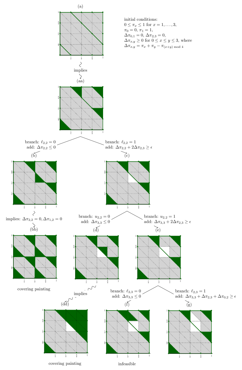
Figure 10 shows a tree of prescribed partial paintings of $\Delta\mathcal{P}_{\frac{1}{q}\mathbb{Z}}$ with $q=4$ and $f=\frac{1}{4}$, obtained from branching on the variables $\ell_{x,y}$ and $u_{x,y}$. In (the upper left triangular part of) the partial painting at its root node (a), the values of the following binary variables are set to $0$.

$$p_{0,0},\;p_{0,1},\;p_{0,2},\;p_{0,3},\;p_{2,3},\;v_{0,0},\;v_{0,1},\;v_{0,2},\;v_{0,3},\;d_{0,0},\;d_{1,3},\;d_{2,2}.$$

3.3. Function value variables

The values of candidate functions are modeled by continuous variables $\pi_{0},\pi_{1},\dots,\pi_{q-1}\in[0,1]$. They are subject to the constraints in Theorem 2.2.

$$\pi_{0}=0$$ (7a)

$$\epsilon\,p_{x,y}\leq\pi_{x}+\pi_{y}-\pi_{(x+y)\bmod q}\leq 2p_{x,y}$$ (7b)

$$\pi_{x}+\pi_{(qf-x)\bmod q}=1,$$ (7c)

where $\epsilon$ is a small positive number used to enforce the strict subadditivity of vertices $(x,y)$ with $p_{x,y}=1$. See section 3.6 for a further discussion on the value of $\epsilon$.

3.4. Slope value variables and assignment

In a search for functions with a prescribed number $k$ of different slopes, we introduce $k$ continuous variables $s_{1},s_{2},\dots,s_{k}\in[-q,q]$ for the different slope values of $\pi$. We can enforce $s_{1}>s_{2}>\dots>s_{k}$ by another artificial lower bound $\epsilon^{\prime}$ (see section 3.6):

$$s_{j}-s_{j+1}\geq\epsilon^{\prime},\text{ for }1\leq j\leq k-1.$$ (8a)

Then binary variables $$\delta_{x,j} 0\leq x\leq q-1,1\leq j\leq k$$ () are used to assign intervals to slope values:

$$\sum_{j=1}^{k}{\delta_{x,j}=1},\text{ for }0\leq x\leq q-1,$$ (8b)

$$s_{j}=q(\pi_{x+1}-\pi_{x})\text{ if and only if }\delta_{x,j}=1,\text{ for }0\leq x\leq q-1\text{ and }1\leq j\leq k.$$

The last condition can be written as the linear inequality

$$\left|s_{j}+q(\pi_{x}-\pi_{x+1})\right|\leq 2q(1-\delta_{x,j}).$$ (8c)

We add the linear constraints

$$\sum_{x=0}^{q-1}\delta_{x,j}\geq 1,\text{ for }1\leq j\leq k$$ (8d)

to the MIP formulation, so as to ensure that every slope value $$s_{j}$$ is used by at least one interval.

3.5. Variables for directly and indirectly covered intervals

We use binary variables $c_{z,0}$ ($0\leq z\leq q-1$) to control whether the interval $[\frac{z}{q},\frac{z+1}{q}]$ is directly covered or not: $0$ for covered and $1$ for uncovered. They are subject to combinatorial conditions of being directly covered by dark green triangles presented in section 3.1. For $0\leq z\leq q-1$, we have that $c_{z,0}=0$ if and only if at least one of the following binary variables has value $0$.

$$\ell_{z,y}\;(0\leq y\leq q-1),\quad u_{z,y}\;(0\leq y\leq q-1),$$ (9a)

$$\ell_{x,z}\;(0\leq x\leq q-1),\quad u_{x,z}\;(0\leq x\leq q-1),$$ (9b)

$$\ell_{x,y}\;(0\leq x,y\leq q-1\text{ such that }x+y\equiv z\pmod{q}),$$ (9c)

$$u_{x,y}\;(0\leq x,y\leq q-1\text{ such that }x+y+1\equiv z\pmod{q})$$ (9d)

We assume that the saturation process of transferring indirectly covered properties described in section 3.1 ends in a finite number maxstep of steps. (Though no theoretical bound better than $\texttt{maxstep}\leq q$ is known, in practice a small value of maxstep such as 2 is sufficient.) For $1\leq i\leq\texttt{maxstep}$, we define binary variables $c_{z,i}$ ($0\leq z\leq q-1$) to model whether the interval $[\frac{z}{q},\frac{z+1}{q}]$ is covered in the first $i$ steps of the saturation process. If the interval $[\frac{z}{q},\frac{z+1}{q}]$ was already covered in the step $i-1$, then it remains covered in the step $i$. Thus, we have the constraint

$$c_{z,i-1}=0\Rightarrow c_{z,i}=0.$$ (10a)

If the interval $$[\frac{z}{q},\frac{z+1}{q}] [\frac{x}{q},\frac{x+1}{q}] i-1 [\frac{z}{q},\frac{z+1}{q}] i$$ is connected by a green edge to an interval that was already covered in the step , then the interval becomes covered in the step .

$$\min\{d_{x,z},h_{x,(z-x)\bmod q},v_{(x-z)\bmod q,z}\}=0\text{ and }c_{x,i-1}=0\Rightarrow c_{z,i}=0.$$ (10b)

Otherwise $c_{z,i}=1$.

Note that these constraints can all be expressed using linear equations or inequalities over binary variables.

3.6. Trade-off between strictness and basicness

Assume that the variables and the constraints defined in section 3.4 were not introduced to our MIP, and that the strict subadditivity constraints were not enforced (i.e., set $\epsilon=0$ in (7b)).

Remark 3.1.

Painting faces dark green in $\Delta\mathcal{P}_{\frac{1}{q}\mathbb{Z}}$ (i.e., setting binary variables $p_{x,y}$ to $0$) amounts to restricting the corresponding subadditivity inequalities (2) of Theorem 2.2 to equations in the constraint system of the polytope $\Pi_{f}(\tfrac{1}{q}\mathbb{Z}/\mathbb{Z})$ of minimal functions. Thus, the set of restricted functions $\pi|_{\frac{1}{q}\mathbb{Z}}$ that satisfy the new constraint system is a smaller polytope, which is a face of the polytope $\Pi_{f}(\frac{1}{q}\mathbb{Z}/\mathbb{Z})$. A vertex of the smaller polytope is also a vertex of the polytope $\Pi_{f}(\frac{1}{q}\mathbb{Z}/\mathbb{Z})$.

After fixing $0/1$ variables, a basic feasible solution $\pi$ of the system with $c_{z,\texttt{maxstep}}=0$ for $0\leq z\leq q-1$ is extreme for $R_{f}(\mathbb{R}/\mathbb{Z})$, according to Theorem 3.1. Unfortunately, in this case we cannot expect the solutions returned by the MIP solver to always have $k$ different slope values; indeed, they often degenerate to 2-slope or 3-slope functions. The same phenomenon was observed in the shooting experiments in the literature [22, 16, 32], where the extreme functions that received a large percentage of hits are 2-slope or 3-slope functions.

Because of this, we use the slope value variables and constraints from section 3.4 in the MIP, always enforcing the strict inequality in slope variables by making a practical choice of $\epsilon^{\prime}>0$ for (8a). In this way we can set the number of slopes $k$ of the resulting functions explicitly. We also use $\epsilon>0$ in (7b), which allows for a significant speedup.

Remark 3.1.

2.2 shows that we do not lose any extreme functions by setting $0<\epsilon,\epsilon^{\prime}\leq 10^{-{q}/{4}}$. Our code instead uses the heuristic choice $\epsilon=\epsilon^{\prime}=1/4$ (or $1/12$), which allows for stronger pruning based on linear programming at the expense of losing some functions.

However, now a basic feasible solution of the system after fixing $0/1$ variables is no longer guaranteed to be an extreme function, since the smaller polytope with the inequalities $\pi_{x}+\pi_{y}-\pi_{(x+y)\bmod q}\geq\epsilon$ is not a face of the polytope $\Pi_{f}(\tfrac{1}{q}\mathbb{Z}/\mathbb{Z})$. In this case, a further extremality test needs to be applied to the returned candidate function $\pi$. Since all intervals are covered (i.e., $c_{z,\texttt{maxstep}}=0$ for $0\leq z\leq q-1$), it suffices by Theorem 3.1 to test whether $\pi|_{\frac{1}{q}\mathbb{Z}}$ is a vertex of $\Pi_{f}(\frac{1}{q}\mathbb{Z}/\mathbb{Z})$.

3.7. Objective function

A tailored objective function can be used to steer the optimum away from equality of slopes and from the lower bounds of the subadditivity slacks $\Delta\pi_{x,y}$, ensuring that the basic optimal solution returned by the MIP solver will correspond to an extreme function. However, there is no a priori best choice of such an objective function that will guarantee success. In our computations, we always maximize the difference of slopes $s_{1}-s_{k}$. Other objective functions, including the following, are plausible:

• maximize a weighted difference of slopes $\displaystyle\sum_{j=1}^{k-1}{\lambda_{j}(s_{j}-s_{j+1})}$, for some suitable weights $\lambda_{j}$;

• maximize a weighted sum of subadditivity slacks $\displaystyle\sum_{0\leq x\leq y\leq q-1}{\omega_{x,y}\Delta\pi_{x,y}}$;

• maximize a weighted sum of subadditivity points $\displaystyle\sum_{0\leq x\leq y\leq q-1}{\omega_{x,y}p_{x,y}}$;

• minimize the covering count $\displaystyle\sum_{0\leq x,y\leq q-1}{u_{x,y}+\ell_{x,y}}$.

3.8. Implementation and discussion

The MIP approach is easy to implement and also easy to tailor to a search for extreme functions with particular properties.

However the approach is limited because floating-point implementations are not a good match for finding functions of high arithmetic complexity. If $q$ is large, the difference between two slope values $s_{i}$ often becomes extremely small and may completely disappear in floating point fuzz, making the choice of the parameter $\epsilon^{\prime}$ difficult.

Moreover, MIP solvers are generally not the best tool for performing an exhaustive search. While listing several solutions should be possible by varying the objective function, this is rather difficult to do in practice. We have used the solver Gurobi (version 5.6.3) to solve the MIP problem. We resorted to setting the Gurobi parameter SolutionLimit=1 and calling optimize() repeatedly, so that the feasible solutions found by Gurobi before reaching the global optimal solution are recorded.

Despite these limitations, we have obtained new results with the MIP approach, which we report in the next two subsections.

3.9. Result: Optimality of the oversampling factor $3$

Using the MIP approach described above, we found an example to answer an open question in [8]. The open question relates to the following theorem.

Theorem 3.2 ([9, Theorem 8.6]).

Let $m\geq 3$, the oversampling factor, be a positive integer. Let $\pi$ be a continuous piecewise linear minimal valid function for $R_{f}(\mathbb{R}/\mathbb{Z})$ with breakpoints in $\tfrac{1}{q}\mathbb{Z}$ and suppose $f\in\tfrac{1}{q}\mathbb{Z}$. The following are equivalent:

1. $\pi$ is a facet for $R_{f}(\mathbb{R}/\mathbb{Z})$,

2. $\pi$ is extreme for $R_{f}(\mathbb{R}/\mathbb{Z})$,

3. $\pi|_{\frac{1}{mq}\mathbb{Z}}$ is extreme for $R_{f}(\tfrac{1}{mq}\mathbb{Z}/\mathbb{Z})$.

Dey et al. [15] gave a function $\pi=\texttt{\href https://github.com/mkoeppe/infinite-group-relaxation-code/search?q=$ that is not extreme for $R_{f}(\mathbb{R}/\mathbb{Z})$, but $\pi|_{\frac{1}{q}\mathbb{Z}}$ is extreme $R_{f}(\tfrac{1}{q}\mathbb{Z}/\mathbb{Z})$. Thus, Theorem 3.2 does not hold with the oversampling factor $m=1$. Basu et al. [7] proved Theorem 3.2 for an oversampling factor $m=4$. It was strengthened to any $m\geq 3$ in [9]. The question whether $m\geq 3$ is best possible or can be improved to $m=2$ was stated in [8, Open Question 8.7]. We resolve this question by the following result, which was stated in the introduction as 1.1.

Proposition 3.2.

The lower bound $m\geq 3$ for the oversampling factor in Theorem 3.2 is best possible. Theorem 3.2 does not hold when $m=2$.

Unable to construct an example function by hand, we established this result by using the MIP approach. Before we explain the details of the search strategy, we describe the structure of the example function that we found, kzh_2q_example_1. It is a continuous $4$-slope function with $q=37$ and $f=\tfrac{25}{37}$; see Figure 4. One can verify, simply using the automated extremality test implemented in the software [23], that kzh_2q_example_1 is a non-extreme function, whose restriction to $\frac{1}{2q}\mathbb{Z}$ is extreme. This proves that an oversampling factor of 3 is optimal.

In the following, we provide a brief justification of the extremality result given by the code. It connects to the theory of equivariant perturbations developed in [7].

Proof of 3.2.

We show that the function $\pi$ is not extreme for $R_{f}(\mathbb{R}/\mathbb{Z})$, by computing the covered intervals. It can be verified on the complex $\Delta\mathcal{P}_{\frac{1}{q}\mathbb{Z}}$ that

1. the intervals $[\tfrac{10}{37},\tfrac{11}{37}]$ and $[\tfrac{14}{37},\tfrac{15}{37}]$, indicated by yellow strips in Figure 4, are uncovered;

2. the others intervals are covered.

There exists thus a non-zero perturbation function $\bar{\pi}$, such that $\pi=\tfrac{1}{2}\pi^{1}+\tfrac{1}{2}\pi^{2}$ where $\pi^{1}=\pi+\bar{\pi}$, $\pi^{2}=\pi-\bar{\pi}$ are two distinct minimal functions, showing the non-extremality of $\pi$ for $R_{f}(\mathbb{R}/\mathbb{Z})$. The function plotted in magenta in Figure 4 is such a function $\bar{\pi}$.

By [7, Definition 3.3, Lemma 2.7 and Theorem 4.6], a perturbation function $\bar{\pi}$ is affine linear on the covered intervals, and satisfies $\bar{\pi}(0)=\bar{\pi}(f)=\bar{\pi}(1)=0$, $\Delta\bar{\pi}(x,y)=0$ for any $(x,y)$ such that $\Delta\pi(x,y)=0$. Consider the restriction to $\frac{1}{q}\mathbb{Z}$. One can show by linear algebra that the finite dimensional linear system has a unique solution $\bar{\pi}|_{\frac{1}{q}\mathbb{Z}}=0$. It follows that $\bar{\pi}$ can only be non-zero on the uncovered intervals, i.e., on $[\tfrac{10}{37},\tfrac{11}{37}]$ and $[\tfrac{14}{37},\tfrac{15}{37}]$. Furthermore, $\pi|_{\frac{1}{q}\mathbb{Z}}$ is extreme for $R_{f}(\frac{1}{q}\mathbb{Z}/\mathbb{Z})$.

Next, we will show that $\pi|_{\frac{1}{2q}\mathbb{Z}}$ is extreme for $R_{f}(\frac{1}{2q}\mathbb{Z}/\mathbb{Z})$. Again it can be verified that

1. $F([\tfrac{10}{37},\tfrac{11}{37}],\{\frac{4}{37}\},[\tfrac{14}{37},\tfrac{15}{37}])$ is an additive edge of $\Delta\mathcal{P}_{\frac{1}{q}\mathbb{Z}}$.

In other words, for $x\in[\tfrac{10}{37},\tfrac{11}{37}]$, we have $\Delta\pi(x,\frac{4}{37})=0$, and thus $\Delta\bar{\pi}(x,\frac{4}{37})=0$. Following [7], for $t\in\mathbb{R}$, define the translation $\tau_{t}\colon\mathbb{R}\to\mathbb{R}$, $x\mapsto x+t$. The gold-colored single headed arrow in Figure 4 indicates the action of translation $\tau_{4/37}$, which sends the interval $[\tfrac{10}{37},\tfrac{11}{37}]$ to the interval $[\tfrac{14}{37},\tfrac{15}{37}]$. Therefore, $\bar{\pi}(\tau_{4/37}(x))=\bar{\pi}(x)+\bar{\pi}(\tfrac{4}{37})=\bar{\pi}(x)$ for $x\in[\tfrac{10}{37},\tfrac{11}{37}]$, as $\bar{\pi}(\tfrac{4}{37})=0$. In particular, we have $\bar{\pi}(\tfrac{21}{74})=\bar{\pi}(\tfrac{29}{74})$. For $r\in\mathbb{R}$, define the reflection $\rho_{r}\colon\mathbb{R}\to\mathbb{R}$, $x\mapsto r-x$. The gold-colored double-headed arrow in Figure 4 indicates the action of reflection $\rho_{f}$ between the two uncovered intervals, corresponding to the symmetry condition $\pi(x)+\pi(f-x)=\pi(f)=1$ for $x\in[\tfrac{10}{37},\tfrac{11}{37}]$. We have $\bar{\pi}(x)+\bar{\pi}(\rho_{f}(x))=\bar{\pi}(f)=0$ for $x\in[\tfrac{10}{37},\tfrac{11}{37}]$. In particular, $\bar{\pi}(\tfrac{21}{74})+\bar{\pi}(\tfrac{29}{74})=0$. Therefore, $\bar{\pi}(\tfrac{21}{74})=\bar{\pi}(\tfrac{29}{74})=0$, the perturbation function $\bar{\pi}$ has values zero at the midpoints of the two uncovered intervals. Since $\bar{\pi}=0$ on the other intervals which are covered, we have $\bar{\pi}|_{\frac{1}{2q}\mathbb{Z}}=0$. Hence, $\pi|_{\frac{1}{2q}\mathbb{Z}}$ is extreme for $\smash[t]{R_{f}(\frac{1}{2q}\mathbb{Z}/\mathbb{Z})}$. ∎

Our tailored MIP search strategy was to look for functions with properties (i–iii) from the above proof. These properties correspond to a prescribed partial painting and thus can be expressed by fixing some binary variables. We tried out various pairs of $(q,f)$ for $10\leq q\leq 40$. For $q=37$ and $f=\frac{25}{37}$, we discovered the function kzh_2q_example_1.

3.10. Result: Refutation of the generic 4-slope conjecture

Our search also resolves [8, Open Question 2.16] by showing that even for functions whose extremality proof only uses the Interval Lemma, rather than the more general techniques from [7] (translations and reflections), many slopes are possible. This is in contrast to the first 5-slope functions found by Hildebrand (2013, unpublished), whose extremality proof requires translating and reflecting covered intervals.

Proposition 3.2.

There exists a piecewise linear extreme function $\pi$ of $R_{f}(\mathbb{R}/\mathbb{Z})$ with more than 4 slopes, such that its additivity domain $E(\pi):=\left\{\,(x,y):\Delta\pi(x,y)=0\,\right\}$ is the union of full-dimensional convex sets and the lines $x\in\mathbb{Z}$, $y\in\mathbb{Z}$, $x+y\in f+\mathbb{Z}$.

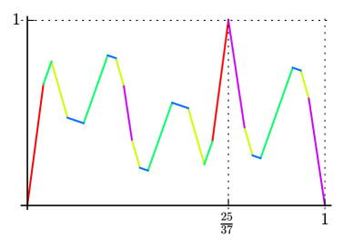
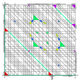
See the functions kzh_5_slope_fulldim_1 etc., which we have made available as part of [35]. They are continuous 5-slope extreme functions without any $0$-dimensional or $1$-dimensional maximal additive faces except for the symmetry reflections $x+y\in f+\mathbb{Z}$ and the trivial additivities $x\in\mathbb{Z}$, $y\in\mathbb{Z}$. A graph of the function kzh_5_slope_fulldim_1 and a plot of its painting on the two-dimensional complex are shown in Figure 9.

Figure 9. The 5-slope extreme function kzh_5_slope_fulldim_1 found by our search code (left). Its two-dimensional polyhedral complex $\Delta\mathcal{P}$ (right), as plotted by the command plot_2d_diagram(h,colorful=True), does not have any lower-dimensional maximal additive faces except for the symmetry reflection or $x=0$ or $y=0$.

Remark 3.2.

Using our computer-based search we also found extreme functions that do have lower-dimensional additive faces, but whose extremality proof does not depend on those. All intervals are directly covered. Examples are provided by the functions kzh_5_slope_fulldim_covers_1, kzh_6_slope_fulldim_covers_1 etc., which we have made available as part of [35].

4. Backtracking search

4.1. Search via covering paintings

In this section we discuss a new search strategy that addresses the limitations of the MIP approach of the previous section by using our own implementation of backtracking tailored to enumerating covering paintings.

During our backtracking search, we maintain a prescribed partial painting as introduced in 3.1. At the root, the minimality conditions (Theorem 2.2)

$$\pi_{0}=0\text{ and }0\leq\pi_{x}\leq 1, \text{ for }x=1,\dots,q-1$$ (11a)

$$\Delta\pi_{x,y}=\pi_{x}+\pi_{y}-\pi_{(x+y)\bmod q}\geq 0, \text{ for }0\leq x\leq y\leq q-1$$ (11b)

$$\pi_{qf}=1\text{ and }\Delta\pi_{x,(qf-x)\bmod q}=0, \text{ for }x=0,\dots,q-1$$ (11c)

give the initial prescribed partial painting on $\Delta\mathcal{P}_{\frac{1}{q}\mathbb{Z}}$. See Figure 10 for an example where $q=4$ and $f=\frac{1}{4}$. To get an extreme function, more additivity relations are needed. To achieve this, in our backtracking search we successively paint some light grey faces white or dark green, until a covering painting is reached. During the painting process, we keep track of the consistency of the colors of the faces by using an LP that will be explained later in section 4.3. If the current partial painting is infeasible, pruning will be performed.

Theorem 3.1 and 2.2 have the following corollary.

Corollary 4.0.

Let $\pi$ be a continuous piecewise linear function with breakpoints in $\tfrac{1}{q}\mathbb{Z}$. If $\pi$ is extreme for $R_{f}(\mathbb{R}/\mathbb{Z})$, then there exists a covering painting such that $\pi|_{\frac{1}{q}\mathbb{Z}}$ is a vertex of the polytope formed by the minimal functions for $R_{f}(\frac{1}{q}\mathbb{Z}/\mathbb{Z})$ whose additivities correspond to the painting.

The search for extreme functions $\pi$ is thus converted into the search for covering paintings.

4.2. Branching rule

The search tree has a binary structure. Assume that we are branching on a triangle $F$ (say the lower triangle whose lower left corner is vertex $(x,y)$) that is colored (light) grey in the partial painting of the current node. In terms of section 3, the value of $\ell_{x,y}$ is undecided. Branching on the node creates two children: one where the triangle $F$ is painted dark green ($\ell_{x,y}$ is set to $0$) and one where (the interior of) $F$ is painted white ($\ell_{x,y}$ is set to $1$).

In the child node with dark green $F$, the following additivity constraints hold.

$$\Delta\pi_{u,v}=0,\quad\text{ for every vertex }(u,v)\text{ of }F.$$ (12)

In the child node with white $F$, the following strict subadditivity relation holds:

$$\sum_{\text{vertex }(u,v)\text{ of }F}\Delta\pi_{u,v}>0.$$

Since the strict inequality constraints are not allowed in linear programming, we prefer to replace it by

$$\sum_{\text{vertex }(u,v)\text{ of }F}\Delta\pi_{u,v}\geq\epsilon,$$ (13)

where $\epsilon$ is a small positive number. See 3.1 for the value of $\epsilon$.

Figure 10. A tree of partial paintings of $\Delta\mathcal{P}_{\frac{1}{4}\mathbb{Z}}$ with $f=\frac{1}{4}$.

4.3. Feasibility and satisfiability checks

To check the feasibility of a prescribed partial painting and detect its implied additivity relations, we use linear programming. We have investigated two options. As we mentioned before, SageMath has a good interface to the Parma Polyhedra Library. Its implementation of the double description method provides an attractive interface to checking feasibility and for testing implied additivities, all in exact arithmetic. This approach, however, appears to be quite slow when the dimension of the polytope is large. As a rule of thumb, when the dimension exceeds $9$, it is better to apply the simplex method instead. Our search code uses the GLPK solver, which is integrated well in SageMath (see section A.2 for details), and allows for warm-starting the simplex method.

We construct the linear optimization problem as follows. The problem has $q$ real variables $\pi_{0},\dots,\pi_{q-1}$, and some auxiliary variables $\Delta\pi_{x,y}$ ($0\leq x\leq y\leq q-1$) that represent the subadditivity slacks. The initial constraints on the variables are given in (11). The subadditivity and additivity constraints are reflected by the bounds of their slack variables. These bounds will vary along the backtracking process. If we walk downwards in the tree, then we append either (12) or (13) to the constraint system; conversely, if we walk upwards in the tree, then we remove the constraint.

Such changes in the constraint system could affect the feasibility of the problem. Due to the update of the variable bounds, the dual simplex method starting off the last basis is called to check whether the partial painting remains feasible at the current node. If the node is infeasible, the whole sub-tree will be pruned. For example, the node (f) in Figure 10 is infeasible, as $\Delta\pi_{3,3}\leq 0$ and $\Delta\pi_{3,3}\geq\epsilon>0$.

The current constraint system may imply some new additive faces in the prescribed partial painting. To check if a vertex $(u,v)$ is implied additive, we call the primal simplex method starting off the last basis to maximize the objective function $\Delta\pi_{u,v}$. If the optimal value is $0$, then $\Delta\pi_{u,v}=0$ and thus the vertex $(u,v)$ is implied additive (dark green). In terms of section 3, $p_{u,v}=0$. Subject to the inclusion constraints (6), the colors of edges and triangles are updated accordingly. See the nodes (bb) and (dd) in Figure 10 for examples.

4.4. Heuristic choice of the branching triangle

By the invariance of the subadditivity condition under exchanging $x$ and $y$, only the upper left triangular part of the complex $\Delta\mathcal{P}_{\frac{1}{q}\mathbb{Z}}$ needs to be considered for painting.

In our experiments we found that an exhaustive search of all paintings of the two-dimensional complex is too expensive even for a moderate size of $q$. Thus, to reach a covering painting quickly, we branch on the colors of the triangles ($\ell_{x,y}$ and $u_{x,y}$) rather than on the colors of the vertices ($p_{x,y})$. Furthermore, a heuristic painting strategy is applied: While picking a light grey triangle to paint dark green or white in branching, we consider those triangles $F$ whose projections $p_{1}(F)$ and $p_{2}(F)$ are currently uncovered. This is of course restrictive, and so we cannot guarantee that our search code will find all covering paintings and all extreme functions. However, it has proved to be a successful heuristic strategy.

At each node, we choose one candidate triangle $F$ (i.e., one $\ell_{x,y}$ or $u_{x,y}$ variable) among all these considered triangles. It is defined as the smallest triangle in lexicographical order, whose color has not been branched on yet in the search tree.

4.5. Incremental computation

For the purpose of improving the running time efficiency, all computations in the backtracking search, such as updating covered intervals, are done in an incremental manner.

More precisely, we maintain a list of connected components that we have mentioned in section 3.1. When a new triangle $F$ is painted as additive in the prescribed partial painting, the components that contain the projection $p_{1}(F)$ or $p_{2}(F)$ or $p_{3}(F)$ are merged into one big component, and all intervals in this new component become covered. When a new edge (one-dimensional face) $F$ is painted as additive (dark green), the components that contain its projection intervals are merged into one big component. If the new component contains an interval that was covered, then all intervals in this new component are covered. In such a way, the new covered intervals after adding an additive face can be computed incrementally from the covered intervals in the previous step. For example, the node (a) in Figure 10 has three connected components $\mathcal{C}_{1}=\{[0,\frac{1}{4}]\}$, $\mathcal{C}_{2}=\{[\frac{1}{4},\frac{1}{2}],[\frac{3}{4},1]\}$ and $\mathcal{U}=\{[\frac{1}{2},\frac{3}{4}]\}$, where the first two are covered and the last one is not. When $\ell_{2,2}$ is set to $0$ in its child (b), $\mathcal{U}$ is merged into $\mathcal{C}_{1}$, and becomes covered. Thus, the node (b) has two connected components $\mathcal{C}_{1}^{\prime}=\{[0,\frac{1}{4}],[\frac{1}{2},\frac{3}{4}]\}$ and $\mathcal{C}_{2}=\{[\frac{1}{4},\frac{1}{2}],[\frac{3}{4},1]\}$ that are both covered.

We mentioned above that a function $\pi$ whose additivities satisfy the prescribed partial painting has the same slopes on the intervals in each component, see [7, Remark 3.6]. By counting the connected components, we get an upper bound on the number of slopes that the function $\pi$ could have. This allows us to prune subtrees that cannot contain functions with the desired number of slopes.

The knowledge of connected components is also used at the end of “vertex filtering mode” (section 2), to check efficiently whether all intervals are covered, as follows. If an interval $[\frac{z}{q},\frac{z+1}{q}]$ does not belong to any covered connected component from the partial painting and if none of the values (9) is $0$, then $\pi$ has uncovered interval and hence is not extreme. This saves us from running the full extremality test on $\pi$, which would consume more time according to Figure 5–middle.

4.6. Heuristic search algorithm

We summarize the backtracking search via covering paintings in Algorithm 2. It is referred to as the “heuristic mode” search in our code.

1. The root node is the initial painting given by the minimality conditions (11);

2. Decide for a candidate triangle $F$ of the painting using covered intervals;

3. A node is branched into two child nodes:

4. For the child node in which $F$ is additive (dark green),

   • add the new additivity relations (12) to constraints;

   • look for implied additive vertices and triangles;

   • update covered intervals;

   • if the node is infeasible, backtrack;

   • if the number of the connected components is less than the desired number of slopes, backtrack;

   • if a covering painting is found, output it and backtrack;

5. For the sub-node in which $F$ is strictly subadditive (white),

   • add the strict subadditivity relation (13) to constraints;

6. Traverse the search tree in depth-first order.

Algorithm 2 heuristic mode

For each covering painting returned by the algorithm, we use the minimality conditions (11) and the additivity relations $\Delta\pi_{x,y}=0$ specified by the green vertices $(x,y)$ in the painting, to construct a polytope. (The strict subadditivity constraints $\Delta\pi_{x,y}>0$ corresponding to the green vertices $(x,y)$ in the painting are neglected.) We enumerate the vertices of the polytope. By 3.1 and Theorem 3.1, the interpolation $\pi$ of a vertex $\pi|_{\frac{1}{q}\mathbb{Z}}$ is extreme for $R_{f}(\mathbb{R}/\mathbb{Z})$.

4.7. Combined search algorithm

The above search algorithms work well for relatively small $q$, but become inefficient when $q$ is large: The vertex filtering search (Algorithm 1) wastes time on enumerating numerous vertex-functions in high dimension, most of which are non-extreme for the infinite group problem; the heuristic backtracking search via covering paintings (Algorithm 2) suffers from the combinatorial explosion in branching and the general performance penalty from using Python.

We propose to combine the vertex filtering search and the heuristic backtracking search to obtain a better performance. The combined algorithm starts with branching, but outputs the partial painting and backtracks at a certain depth before reaching a covering painting. For each generated partial painting, the algorithm constructs the polytope as described in section 4.6 and then performs a vertex enumeration as described in the vertex filtering search. It remains to determine a good stopping criterion for branching.

Since the vertex enumeration algorithm has a good performance for low-dimensional polytopes, we wish to use the dimension as the stopping criterion. However the actual dimension of the polytope given by a painting is unknown, unless it has been constructed, when it is too late. Therefore, instead of the actual dimension, we use expected dimension as the stopping criterion in our code. This expected dimension can be computed efficiently without calling PPL to construct the polytope. We set up a $q$-column matrix (cs_matrix) to record the equality constraints on $(\pi_{0},\dots,\pi_{q})$, which are $\pi_{0}=0$, the symmetry constraints and the additivity constraints specified by the painting. The matrix is maintained dynamically during the backtracking process. Define the expected dimension to be the co-rank of the equation system: $\texttt{exp\char 95\relax\allowbreak dim}:=q-\operatorname{rk}(\texttt{cs\char 95\relax\allowbreak matrix})$.

The algorithm switches from backtracking to vertex enumeration once the expected dimension becomes smaller than a certain threshold. Table 4 shows that a value around $11$ is the best empirical threshold for finding an extreme function with many slopes quickly.

The combination of vertex filtering search and heuristic backtracking search produces a more powerful search algorithm, which is called “combined mode” in our code. We summarize it as Algorithm 3.

1. Run the heuristic search (Algorithm 2), with one more stopping criterion added to its step 4:

   • append the new equations to cs_matrix;

   • compute $\texttt{exp\char 95\relax\allowbreak{}dim}:=q-\operatorname{rk}(\texttt{cs\char 95\relax\allowbreak{}matrix})$;

   • if exp_dim $\leq$ threshold (empirically, threshold $=11$),

output the partial painting and backtrack;

For each partial painting returned by phase 1, construct the corresponding polytope and run the vertex filtering search (Algorithm 1, steps 3–4).

Algorithm 3 combined mode

4.8. Results

Using the combined search (Algorithm 3), our code was able to find up to 7-slope extreme functions for $q\leq 34$, namely kzh_7_slope_1 to kzh_7_slope_4.

Table 4. Vertex enumeration in high dimension vs. Combinatorial explosion in branching

	$q=25$			$q=26$		$q=27$		$q=28$		$q=29$		$q=30$		$q=31$
$k$	6	6	6	6	6	6	6	6	6	6	7	7	6	7	7
$f$	1	7	8	1	9	1	9	1	9	1	10	1	10	1	10
	number of $\geq k$-slope solutions
	2	1	1	8	4	14	1	26	17	60	1	3	30
	running time (s) in vertex filtering search
v-enumeration	59	40	28	375	322	439	706	3866	3806	3728	3626	23642	2880
first solution	86	42	47	378	330	440	757	3873	3845	3739	3650	23747	2889
all solutions	92	63	51	454	370	555	818	4211	4049	4369	3958	24506	3256
threshold	running time (s) in combined search to find the first $\geq k$-slope solution
05	6	122	666	5	1369	20	1932	282	2875	20	7809	1884	5896	05181	35455
06	4	066	397	3	0921	14	1322	064	2084	12	6278	1587	1529	04527	24243
07	3	032	224	2	0518	11	0845	055	1292	15	4807	1492	1031	05728	19043
08	3	013	121	5	0267	20	0641	101	0779	15	4823	3782	0449	21821	08604
09	1	004	056	5	0135	20	0352	049	0516	02	3194	2032	0242	24822	05487
10	1	004	015	4	0018	05	0121	047	0150	01	1460	0549	0099	08260	02577
11	2	004	015	4	0039	05	0082	027	0029	45	1000	0271	0040	01010	01430
12				4	0038	05	0083	028	0029	44	0932	0306	0040	02352	01186
13								027	0028	46	0928	0308	0042	01269	03365
14												0229	0041	01227	03637

5. Targeted search for extreme functions with many slopes

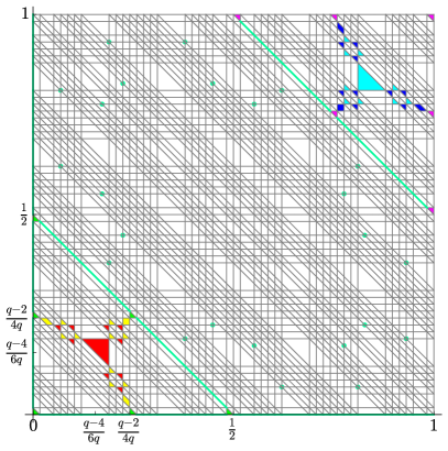
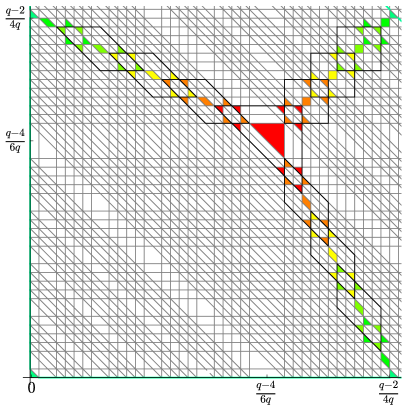
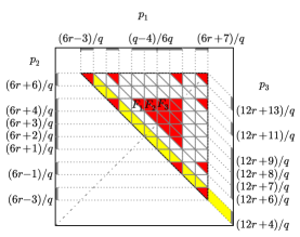
We observed that many of these newly discovered extreme functions with many slopes possess the invariance: $f=1/2$ and $\pi_{i}=\pi_{q-i}$ ($0\leq i\leq q/2$). Targeting the search to functions with the invariance property allowed us to find more new extreme functions with many slopes whose values of $q$ were twice as large as before. In addition, their painting on the complex $\Delta\mathcal{P}_{\frac{1}{q}\mathbb{Z}}$ often includes special patterns, as shown by Figure 11 for example.

Figure 11. Special patterns on the two-dimensional polyhedral complex $\Delta\mathcal{P}_{\frac{1}{q}\mathbb{Z}}$. Left, the $\Delta\mathcal{P}_{\frac{1}{q}\mathbb{Z}}$ of the $6$-slope extreme function kzh_6_slope_1 with $q=58$. We observe that the additive triangles are located in the lower left and upper right corners. The function has the same slopes on the intervals that are projections of the same color additive triangles. The 6-pointed star patterns appear several times. Right, the lower-left corner of $\Delta\mathcal{P}_{\frac{1}{q}\mathbb{Z}}$ of the $10$-slope extreme function kzh_10_slope_1 with $q=166$, where we see that the 6-pointed stars are actually the result of additivity patterns within certain intersecting quadrilaterals (black), which connect like links of three chains. The detailed structure is described in Figure 12.

5.1. Construction of a family of prescribed partial paintings

We then targeted the search to functions for larger values of $q$ with prescribed partial paintings that mimic these patterns. Let $q=36r+22$, where $r\in\mathbb{Z},r\geq 1$. We construct the prescribed partial painting on the complex $\Delta\mathcal{P}_{\frac{1}{q}\mathbb{Z}}$ in $2(r+2)$ steps as follows.

Step $0$: Paint the lower triangles whose lower left corners are the vertices ${\bigl{(}\begin{smallmatrix}0\vphantom{/}\\ 0\vphantom{/}\end{smallmatrix}\bigr{)}},{\bigl{(}\begin{smallmatrix}0\vphantom{/}\\ (q-2)/4q\vphantom{/}\end{smallmatrix}\bigr{)}},{\bigl{(}\begin{smallmatrix}0\vphantom{/}\\ (q-2)/2q\vphantom{/}\end{smallmatrix}\bigr{)}},{\bigl{(}\begin{smallmatrix}(q-2)/4q\vphantom{/}\\ (q-2)/4q\vphantom{/}\end{smallmatrix}\bigr{)}},{\bigl{(}\begin{smallmatrix}(q-2)/4q\vphantom{/}\\ 0\vphantom{/}\end{smallmatrix}\bigr{)}}$ and ${\bigl{(}\begin{smallmatrix}(q-2)/2q\vphantom{/}\\ 0\vphantom{/}\end{smallmatrix}\bigr{)}}$; this is illustrated in Figure 12–1.

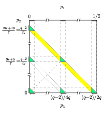
$\Delta\mathcal{P}^{0}$ of Step $0$

$\Delta\mathcal{P}^{1}$ of Step $1$

$\Delta\mathcal{P}^{t}$ of Step $t$

$\Delta\mathcal{P}^{r+1}$ of Step $(r+1)$

Figure 12. Prescribed partial paintings.

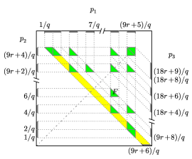
Step $1$: Paint the upper triangles whose upper right corners are the vertices ${\bigl{(}\begin{smallmatrix}i/q\\ j/q\end{smallmatrix}\bigr{)}}$ for ${\bigl{(}\begin{smallmatrix}i\vphantom{/}\\ j\vphantom{/}\end{smallmatrix}\bigr{)}}={\bigl{(}\begin{smallmatrix}2\vphantom{/}\\ 9r+5\vphantom{/}\end{smallmatrix}\bigr{)}},{\bigl{(}\begin{smallmatrix}9r+5\vphantom{/}\\ 9r+5\vphantom{/}\end{smallmatrix}\bigr{)}}$ and ${\bigl{(}\begin{smallmatrix}9r+5\vphantom{/}\\ 2\vphantom{/}\end{smallmatrix}\bigr{)}}$. Paint the lower triangles whose lower left corners are the vertices ${\bigl{(}\begin{smallmatrix}i/q\\ j/q\end{smallmatrix}\bigr{)}}$ for ${\bigl{(}\begin{smallmatrix}i\vphantom{/}\\ j\vphantom{/}\end{smallmatrix}\bigr{)}}={\bigl{(}\begin{smallmatrix}2\vphantom{/}\\ 9r+4\vphantom{/}\end{smallmatrix}\bigr{)}},{\bigl{(}\begin{smallmatrix}4\vphantom{/}\\ 9r+4\vphantom{/}\end{smallmatrix}\bigr{)}},\allowbreak{\bigl{(}\begin{smallmatrix}4\vphantom{/}\\ 9r+2\vphantom{/}\end{smallmatrix}\bigr{)}},\allowbreak{\bigl{(}\begin{smallmatrix}6\vphantom{/}\\ 9r+2\vphantom{/}\end{smallmatrix}\bigr{)}},{\bigl{(}\begin{smallmatrix}9r+2\vphantom{/}\\ 9r+4\vphantom{/}\end{smallmatrix}\bigr{)}},{\bigl{(}\begin{smallmatrix}9r+4\vphantom{/}\\ 9r+4\vphantom{/}\end{smallmatrix}\bigr{)}},{\bigl{(}\begin{smallmatrix}9r+2\vphantom{/}\\ 9r+2\vphantom{/}\end{smallmatrix}\bigr{)}},{\bigl{(}\begin{smallmatrix}9r+4\vphantom{/}\\ 9r+2\vphantom{/}\end{smallmatrix}\bigr{)}},{\bigl{(}\begin{smallmatrix}9r+4\vphantom{/}\\ 4\vphantom{/}\end{smallmatrix}\bigr{)}},{\bigl{(}\begin{smallmatrix}9r+2\vphantom{/}\\ 4\vphantom{/}\end{smallmatrix}\bigr{)}}$ and ${\bigl{(}\begin{smallmatrix}9r+2\vphantom{/}\\ 6\vphantom{/}\end{smallmatrix}\bigr{)}}$; see Figure 12–2.

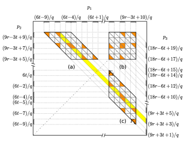
Steps $t=2,3,\dots,r$: Paint the parallelogram whose vertices are ${\bigl{(}\begin{smallmatrix}i/q\\ j/q\end{smallmatrix}\bigr{)}}$ for ${\bigl{(}\begin{smallmatrix}i\vphantom{/}\\ j\vphantom{/}\end{smallmatrix}\bigr{)}}={\bigl{(}\begin{smallmatrix}6t-9\vphantom{/}\\ 9r-3t+10\vphantom{/}\end{smallmatrix}\bigr{)}},{\bigl{(}\begin{smallmatrix}6t-4\vphantom{/}\\ 9r-3t+10\vphantom{/}\end{smallmatrix}\bigr{)}},{\bigl{(}\begin{smallmatrix}6t-4\vphantom{/}\\ 9r-3t+5\vphantom{/}\end{smallmatrix}\bigr{)}},{\bigl{(}\begin{smallmatrix}6t+1\vphantom{/}\\ 9r-3t+5\vphantom{/}\end{smallmatrix}\bigr{)}}$ with the orange pattern shown in Figure 12–3(a)). Paint the square whose vertices are ${\bigl{(}\begin{smallmatrix}i/q\\ j/q\end{smallmatrix}\bigr{)}}$ for ${\bigl{(}\begin{smallmatrix}i\vphantom{/}\\ j\vphantom{/}\end{smallmatrix}\bigr{)}}={\bigl{(}\begin{smallmatrix}9r-3t+5\vphantom{/}\\ 9r-3t+10\vphantom{/}\end{smallmatrix}\bigr{)}},{\bigl{(}\begin{smallmatrix}9r-3t+10\vphantom{/}\\ 9r-3t+10\vphantom{/}\end{smallmatrix}\bigr{)}},{\bigl{(}\begin{smallmatrix}9r-3t+5\vphantom{/}\\ 9r-3t+5\vphantom{/}\end{smallmatrix}\bigr{)}},{\bigl{(}\begin{smallmatrix}9r-3t+10\vphantom{/}\\ 9t-3t+5\vphantom{/}\end{smallmatrix}\bigr{)}}$ with the orange pattern shown in Figure 12–3(b). Paint the parallelogram whose vertices are ${\bigl{(}\begin{smallmatrix}i/q\\ j/q\end{smallmatrix}\bigr{)}}$ for ${\bigl{(}\begin{smallmatrix}i\vphantom{/}\\ j\vphantom{/}\end{smallmatrix}\bigr{)}}={\bigl{(}\begin{smallmatrix}9r-3t+5\vphantom{/}\\ 6t+1\vphantom{/}\end{smallmatrix}\bigr{)}},{\bigl{(}\begin{smallmatrix}9r-3t+5\vphantom{/}\\ 6t-4\vphantom{/}\end{smallmatrix}\bigr{)}},{\bigl{(}\begin{smallmatrix}9r-3t+10\vphantom{/}\\ 6t-4\vphantom{/}\end{smallmatrix}\bigr{)}},{\bigl{(}\begin{smallmatrix}9r-3t+10\vphantom{/}\\ 6t-9\vphantom{/}\end{smallmatrix}\bigr{)}}$ with the orange pattern shown in Figure 12–3(c).

Step $(r+1)$: Paint the triangle whose vertices are${\bigl{(}\begin{smallmatrix}i/q\\ j/q\end{smallmatrix}\bigr{)}}$ for ${\bigl{(}\begin{smallmatrix}i\vphantom{/}\\ j\vphantom{/}\end{smallmatrix}\bigr{)}}={\bigl{(}\begin{smallmatrix}6r-3\vphantom{/}\\ 6r+7\vphantom{/}\end{smallmatrix}\bigr{)}},\allowbreak{\bigl{(}\begin{smallmatrix}6r+7\vphantom{/}\\ 6r+7\vphantom{/}\end{smallmatrix}\bigr{)}},{\bigl{(}\begin{smallmatrix}6r+7\vphantom{/}\\ 6r+3\vphantom{/}\end{smallmatrix}\bigr{)}}$ with the red pattern shown in Figure 12–4.

Step $0$ to Step $(r+1)$ construct the painting on the lower left triangular part of the complex $\Delta\mathcal{P}_{\frac{1}{q}\mathbb{Z}}$. The painting on the upper right triangular part of the complex $\Delta\mathcal{P}_{\frac{1}{q}\mathbb{Z}}$ will then be determined through a mapping. Specifically, in Step $t$ for $t=r+2,r+3,\dots,2r+3$, we paint the triangles whose images under the mapping ${\bigl{(}\begin{smallmatrix}x\vphantom{/}\\ y\vphantom{/}\end{smallmatrix}\bigr{)}}\mapsto{\bigl{(}\begin{smallmatrix}1-x\vphantom{/}\\ 1-y\vphantom{/}\end{smallmatrix}\bigr{)}}$ are colored in Step $(2r+3-t)$. We also paint the diagonal lines $\{{\bigl{(}\begin{smallmatrix}x\vphantom{/}\\ y\vphantom{/}\end{smallmatrix}\bigr{)}}\colon x+y=\tfrac{1}{2},0\leq x\leq\tfrac{1}{2}\}$ and $\{{\bigl{(}\begin{smallmatrix}x\vphantom{/}\\ y\vphantom{/}\end{smallmatrix}\bigr{)}}\colon x+y=\tfrac{3}{2},\tfrac{1}{2}\leq x\leq 1\}$, which correspond to the symmetry condition of minimal valid functions. In the following, we shall refer to the painting constructed as above on $\Delta\mathcal{P}_{\frac{1}{q}\mathbb{Z}}$ as the prescribed partial painting.

5.2. Properties of functions satisfying the prescribed partial paintings

Recall the notion of connected component discussed in section 4.5. Connected components of a painting on $\Delta\mathcal{P}_{\frac{1}{q}\mathbb{Z}}$ are disjoint subsets of $\{[\tfrac{i}{q},\tfrac{i+1}{q}]\colon\allowbreak i=0,1,\dots,q-1\}$. They satisfy the following properties. If $F$ is an elementary upper or lower triangle whose vertices are colored on the painting, then $p_{1}(F),p_{2}(F)$ and $p_{3}(F)$ are in the same connected component. If $F$ is an elementary horizontal, vertical or diagonal edge whose vertices are colored on the painting, then the two intervals among its projections $p_{1}(F),p_{2}(F),p_{3}(F)$ are in the same connected component. In particular, the colored diagonal lines corresponding to the symmetry condition yield that $[\tfrac{i}{q},\tfrac{i+1}{q}]$ and $[\tfrac{j}{q},\tfrac{j+1}{q}]$ are in the same connected component, where $i+j=\tfrac{q}{2}-1=18r+10$.

Lemma 5.0.

Let $q=36r+22$, where $r\in\mathbb{Z},r\geq 1$. Let the prescribed partial painting on $\Delta\mathcal{P}_{\frac{1}{q}\mathbb{Z}}$ be constructed as above. Then all intervals are directly covered. The prescribed partial painting induces exactly $2(r+2)$ connected components.

The proof of this and the following results appears in Appendix C.

Suppose $r\in\mathbb{Z}$, $r\geq 1$, $q=36r+22$ and $f=1/2$. Let $\Pi_{r}$ be the set of continuous piecewise linear minimal valid functions $\pi$ with breakpoints in $\frac{1}{q}\mathbb{Z}$, satisfying in addition the invariance condition $\pi(x)=\pi(1-x)$ for $0\leq x\leq\frac{1}{2}$ and $\Delta\pi(x,y)=0$ for any $0\leq x,y\leq 1$ such that the point $(x,y)$ is colored in the prescribed partial painting on $\Delta\mathcal{P}_{\frac{1}{q}\mathbb{Z}}$.

Clearly we can describe the functions $\pi\in\Pi_{r}$ in the space of the variables $(\pi_{0},\pi_{1},\dots,\pi_{q})$; let us denote the corresponding polytope by $V_{r}$. Due to 5.0, we can describe them also in the space of the slope values $(s_{0},s_{1},\dots,s_{r+1})$ on the connected components; let us denote the corresponding polytope by $S_{r}$. (Note that $s_{t}=-s_{2r+3-t}$ by the invariance condition, for $t=r+2,r+3,\dots,2r+3$.)

Lemma 5.0.

There is a linear isomorphism between the polytope $V_{r}$ in the $(\pi_{0},\pi_{1},\dots,\pi_{q})$ variables and the polytope $S_{r}$ in the $(s_{0},s_{1},\dots,s_{r+1})$ variables.

The proof (in Appendix C) gives an explicit mapping between the values $\pi_{i}$ and the slopes $s_{t}$. With the help of these formulas, we can then show that the slope values are non-increasing.

Lemma 5.0.

Let $s_{0},s_{1},\dots,s_{r+1}$ be as above. Then $s_{0}\geq s_{1}\geq\dots\geq s_{r+1}$.

The computer-based search can now be run in the space of the slope variables $(s_{0},s_{1},\dots,s_{r+1})$, which has the benefit of having a much lower dimension. However, if $r$ is large, the search is still nontrivial. In order to speed up the search we prescribed extra additivity constraints. This approach was successful in finding extreme functions with up to 28 slopes.

Our search also revealed that in general, we cannot expect the existence of an extreme point for which the sequence of slope values is strictly decreasing ($s_{0}>s_{1}>\dots>s_{r+1}$). However, we conclude this section with a weaker conjecture.

Conjecture 5.0.

There exists an extreme point of the polytope $S_{r}$ with $\Omega(r)$ different slope values $s_{i}$.

We abandoned work on this conjecture in late July 2015 when Basu et al. [6] announced a different construction that gives extreme functions with an arbitrary prescribed number of slopes.

5.3. Result: Extreme functions with many slopes

The targeted search was very successful in finding functions with large numbers of slopes. We thus obtained the following result, which we have stated already in the introduction.

Theorem 5.1.

There exist continuous piecewise linear extreme functions with $2$, $3$, $4$, $5$, $6$, $7$, $8$, $10$, $12$, $14$, $16$, $18$, $20$, $22$, $24$, $26$, and $28$ slopes.

Appendix A Implementation details

In this appendix, we describe some aspects of our implementation in SageMath [34], an open-source mathematics software system that uses Python and Cython as its primary programming languages and interfaces with various existing packages.

A.1. SageMath interface for vertex enumeration

PPL is a standard package in SageMath and comes with an efficient Cython interface. Our code uses in particular the class C_Polyhedron for computations with closed convex polyhedra. A polytope can be built starting from a system of constraints cs of class Constraint_System via p = C_Polyhedron(cs), where the constraint system cs is a finite set of linear equality or inequality constraints (class Constraint). One calls p.minimized_generators() to enumerate the vertices of p. PPL also allows for feasibility checks and satisfiability checks (see section 4). The feasibility check can be realized by calling p.is_empty(). The satisfiablity check efficiently tests whether a given inequality or equation c is satisfied by all points in a polytope p. It is accessed by calling p.relation_with(c).implies(Poly_Con_Relation.is_included()).

Once lrslib [2, 3] has been installed as an optional package in SageMath, it is possible to call the programs lrs and redund from SageMath. Our code includes a SageMath interface that reads or writes polytopes in the lrslib format. The lrslib command redund can thus be used in conjunction with PPL as a preprocessor for vertex enumeration.

A.2. SageMath interface for linear programming

We pointed out in section 4.3 the necessity of using an LP solver with warm-starting capability for the feasibility and satisfiability checks described above in the high-dimensional case. We use the SageMath class MixedIntegerLinearProgram as an LP modeling system. Within this framework, a new LP problem m can be created by m = MixedIntegerLinearProgram(maximization=True, solver = "GLPK"), requesting the GLPK solver as its numerical backend. In contrast to other backend implementations, including PPL’s rational LP solver, the GLPK backend has the crucial warm starting capability. We call v = m.new_variable(real=True, nonnegative=True) to define a Python dictionary v of non-negative continuous variables for the problem m. The upper and lower bound of a variable, say v[0], can be changed via m.set_max(v[0], max) and m.set_min(v[0], min) respectively. If the variable is unbounded above or below, then one sets max=None or min=None respectively. The method m.add_constraint(linear_function, max, min) sets up a new constraint $\texttt{min}\leq\texttt{linear\char 95\relax\allowbreak function}\leq\texttt{max}$ for the problem m. The objective function of m is defined by m.set_objective(obj). For a feasibility check, we can use obj=None. We request that GLPK use the simplex method to solve the LP via m.solver_parameter(backend.glp_simplex_or_intopt, backend.glp_simplex_only). According to the setting m.solver_parameter("primal_v_dual", "GLP_PRIMAL") or m.solver_parameter("primal_v_dual", "GLP_DUAL"), the primal or dual simplex method is applied respectively. We call m.solve(objective_only=True) to solve for the optimal value. If it signals a MIPSolverException, then the problem is infeasible.

References:

Appendix B Limitations of search based on $q\times v$ grid discretization

In this section, we discuss limitations of the search based on $q\times v$ grid discretization, an alternative search strategy that was used by Chen [12] and Hildebrand (2013, unpublished).

Consider continuous piecewise linear functions $\pi\colon\mathbb{R}/\mathbb{Z}\to[0,1]$, with breakpoints in $\tfrac{1}{q}\mathbb{Z}$ for some $q\in\mathbb{Z}_{+}$ and $\pi(0)=0$. Suppose without loss of generality that $f\in\tfrac{1}{q}\mathbb{Z}$.

As mentioned in section 1.4, there are two natural ways to discretize the space of functions $\pi$: discretizing function values $\pi_{i}=\pi(\frac{i}{q})$ for $i\in\{0,\dots,q\}$ and discretizing slope values $qs_{i}$ on $[\frac{i-1}{q},\frac{i}{q}]$ for $i\in\{1,\dots,q\}$. See again Figure 2. The following lemma shows that they are equivalent.

Lemma B.0.

Let $v$ be a positive integer. The following are equivalent:

1. $\pi_{i}\in\frac{1}{v}\mathbb{Z}$ for each $i\in\{0,\dots,q\}$.

2. $s_{i}\in\frac{1}{v}\mathbb{Z}$ for each $i\in\{1,\dots,q\}$.

Proof.

Since $\pi_{0}=\pi_{q}=0$ and $s_{i}=\pi_{i}-\pi_{i-1}$ for $i=1,\dots,q$, the lemma follows. ∎

B.1. A lower bound on (a proxy for) arithmetic complexity

In the following, we investigate the worst-case complexity of the search based on $q\times v$ grid discretization, by estimating the arithmetic complexity of extreme functions, i.e., the largest value $v$ needed for any extreme function $\pi$ with breakpoints in $\frac{1}{q}\mathbb{Z}$.

We use the notations $d_{\text{ext}}$, $d_{\text{ver}}$, and $d_{\text{bas}}$, satisfying $d_{\text{ext}}\leq d_{\text{ver}}\leq d_{\text{bas}}$, and the constraint system $A{\mathchoice{\mbox{\boldmath$\displaystyle\bf x$}}{\mbox{\boldmath$\textstyle\bf x$}}{\mbox{\boldmath$\scriptstyle\bf x$}}{\mbox{\boldmath$\scriptscriptstyle\bf x$}}}={\mathchoice{\mbox{\boldmath$\displaystyle\bf b$}}{\mbox{\boldmath$\textstyle\bf b$}}{\mbox{\boldmath$\scriptstyle\bf b$}}{\mbox{\boldmath$\scriptscriptstyle\bf b$}}}$ of the polytope $\Pi_{f}(\frac{1}{q}\mathbb{Z}/\mathbb{Z})$, which were introduced in section 2.6. It is hard to determine the precise value of $d_{\text{ext}}$ as a function of $q$, and we are not able to show an exponential lower bound for it. For estimating the growth rate of $d_{\text{ext}}$, we are satisfied with a simplified study, using $d_{\text{bas}}$ as a proxy. We show the following exponential lower bound.

Lemma B.0.

Let $q\geq 3$ be an odd positive integer. Let $f\in\frac{1}{q}\mathbb{Z}$, $0<f<1$, such that $qf$ and $q$ are coprime integers. Let $A{\mathchoice{\mbox{\boldmath$\displaystyle\bf x$}}{\mbox{\boldmath$\textstyle\bf x$}}{\mbox{\boldmath$\scriptstyle\bf x$}}{\mbox{\boldmath$\scriptscriptstyle\bf x$}}}={\mathchoice{\mbox{\boldmath$\displaystyle\bf b$}}{\mbox{\boldmath$\textstyle\bf b$}}{\mbox{\boldmath$\scriptstyle\bf b$}}{\mbox{\boldmath$\scriptscriptstyle\bf b$}}}$, ${\mathchoice{\mbox{\boldmath$\displaystyle\bf x$}}{\mbox{\boldmath$\textstyle\bf x$}}{\mbox{\boldmath$\scriptstyle\bf x$}}{\mbox{\boldmath$\scriptscriptstyle\bf x$}}}\geq\mathchoice{\mbox{\boldmath$\displaystyle\bf 0$}}{\mbox{\boldmath$\textstyle\bf 0$}}{\mbox{\boldmath$\scriptstyle\bf 0$}}{\mbox{\boldmath$\scriptscriptstyle\bf 0$}}$ be the constraint system of Theorem 2.2 written in the standard form. Then $d_{\mathrm{bas}}$, the maximum absolute value of the determinants of simplex basis matrices of $A$, is at least $2^{\frac{q-1}{2}}$.

Proof.

It suffices to show the existence of a basis matrix $B$ of $A$ with $\mathopen{|}\det B|\geq 2^{\frac{q-1}{2}}$. To find such a $B$, we first prove the following claim. Because $q$ is odd, the operation of multiplying by $2\pmod{q}$ is invertible. For $x\in\{0,1,\dots,q-1\}$, denote the unique $y\in\{0,1,\dots,q-1\}$ satisfying $2y=x\pmod{q}$ by $x/2$.

Claim B.0.

​​  Let $q$ and $f$ be as above. There exists a sequence $(a_{0},a_{1},\dots,\allowbreak a_{q-1})$ of integers with $a_{0}=0$, $a_{1}=qf$ and $a_{2}=qf/2\pmod{q}$ such that the following conditions hold:

1. for odd $i>1$ we have $a_{i}=a_{j}/2\pmod{q}$ for some $j<i$;

2. for even $i>2$ we have $a_{i}=qf-a_{i-1}\pmod{q}$.

3. $\{a_{0},a_{1},\dots,a_{q-1}\}=\{0,1,\dots,q-1\}$.

Proof.

We construct the sequence as follows. Suppose that $a_{0},a_{1},\dots,\allowbreak a_{k}$ are determined for some even $k\geq 2$, such that conditions (1) and (2) are both satisfied for $i\leq k$, and that $a_{0},a_{1},\dots,a_{k}$ are all distinct. Let $S=\{a_{0},a_{1},\dots,a_{k}\}$. We choose $a_{k+1}$ and $a_{k+2}$ by selecting an element $s\in S$ such that $s/2\pmod{q}\notin S$, and then taking $a_{k+1}=s/2\pmod{q}$ and $a_{k+2}=qf-s/2\pmod{q}$. It suffices to show the existence of such an $s\in S$ whenever $S\neq\mathbb{Z}/q\mathbb{Z}$.

Suppose that $s/2\in S$ for every $s\in S$. Since $qf\in S$ and $qf$ and $q$ are coprime, $S$ must contain the coset $qfH=\{qfh:h\in H\}$, where $H$ is the multiplicative subgroup of $(\mathbb{Z}/q\mathbb{Z})^{*}$ generated by $2$. In particular, $qf,2qf\in S$.

By conditions (2) and then (1), we deduce that $S$ also contains $qf-qfH$ and $(qf-qfH)H=qfH-qfH$. Applying this argument repeatedly, we see that $S$ contains $qfH-qfH+qfH-\dots\pm qfH$ for any number of iterations. Since $1,2\in H$, $qfH$ contains $qf$ and $2qf$, and thus any multiple of $qf$ can be written in the form $qfH-qfH+qfH-\dots\pm qfH$. Since $qf$ and $q$ are coprime, we conclude that $S$ contains all of $\mathbb{Z}/q\mathbb{Z}$. ∎

Define the row vectors $R_{0},R_{1},\dots,R_{q-1}\in\mathbb{Z}^{q}$ using the sequence $a_{0},a_{1},\dots,\allowbreak a_{q-1}$ constructed above, as follows. Let $R_{0}$ be the row vector with the only nonzero entry $1$ appearing in the column indexed by $a_{0}=0$, corresponding to the constraint $\pi_{0}=0$. Let $R_{2}$ be the row vector with the only nonzero entry $2$ appearing in the column indexed by $a_{2}$, corresponding to the symmetric constraint $\pi_{a_{2}}+\pi_{a_{2}}=1$. For $i=1$ and $i=4,6,\dots,q-1$, let $R_{i}$ be the row vector with two nonzero entries $1$ appearing in the columns indexed by $a_{i}$ and $a_{i-1}$, corresponding to the symmetric constraint $\pi_{a_{i}}+\pi_{a_{i-1}}=1$. Finally, for $i=3,5,\dots,q-2$, let $R_{i}$ be the row vector with nonzero entry $-2$ at index $a_{i}$ and entry $1$ at index $2a_{i}\pmod{q}$, corresponding to the subadditive constraint $\pi_{a_{i}}+\pi_{a_{i}}\geq\pi_{2a_{i}\bmod q}$.

The basis matrix $B$ is obtained by taking the slack variables for the subadditivity constraints $R_{3},R_{5},\dots,R_{q-2}$ in $A$ as non-basic variables and others as basic variables. To compute $\det B$, first expand out the columns corresponding to slack variables. We are left with a $q\times q$ matrix $B^{\prime}$ consisting of the rows $R_{0},R_{1},\dots,R_{q-1}$, and $\mathopen{|}\det B|=\mathopen{|}\det B^{\prime}|$. See B.0 for the case of $q=11,f=3/11$.

To compute $\det B^{\prime}$, start by expanding along the row $R_{0}$ containing a unique nonzero entry $1$ and end up with a new matrix with this row and column $a_{0}$ removed. In the second step, expand along $R_{1}$, noting that the only nonzero entry remaining in this row is $1$ at column $a_{1}$. We arrive at a new matrix with this row and column $a_{1}$ removed. In the third step, expand along $R_{2}$, noting that the only nonzero entry remaining in this row is $2$ at column $a_{2}$. We then arrive at a new matrix with this row and column $a_{2}$ removed. In general, during the ($k+1$)-st step, we expand along the row $R_{k}$ which contains a unique nonzero entry at column $a_{k}$, whose value is either $-2$ or $1$ depending on whether $k\geq 3$ is even or odd.

The computation terminates in $q$ steps. It follows that $\det B^{\prime}$ is equal to the product of all these unique nonzero entries, $(q-1)/2$ of which are $\pm 2$ and the remaining are $1$. Thus $\mathopen{|}\det B|=2^{\frac{q-1}{2}}$. ∎

Example B.0.

Consider the case $q=11,f=\frac{3}{11}$. By footnote 35, we have the sequence

$$(a_{0},a_{1},\dots,a_{10})=(0,3,7,9,5,10,4,8,6,2,1).$$

The following matrix $B^{\prime}$ is a $q\times q$ submatrix of $A$, where the row $R_{i}$ corresponds to the:

• constraint $\pi_{0}=0$, for $i=0$;

• symmetric constraint $\pi_{a_{2}}+\pi_{a_{2}}=1$, for $i=2$;

• symmetric constraint $\pi_{a_{i}}+\pi_{a_{i-1}}=1$, for $i=1,4,6,\dots,q-1$;

• subadditive constraint $-2\pi_{a_{i}}+\pi_{2a_{i}\text{ mod }q}\leq 0$, for $i=3,5,\dots,q-2$

of $\Pi_{f}(\frac{1}{q}\mathbb{Z}/\mathbb{Z})$.

$$B^{\prime}=\blockarray{c@{\hskip 5.0pt}*{11}r@{\hskip 5.0pt}cl}&\mbox{\scriptsize 0}\mbox{\scriptsize 1}\mbox{\scriptsize 2}\mbox{\scriptsize 3}\mbox{\scriptsize 4}\mbox{\scriptsize 5}\mbox{\scriptsize 6}\mbox{\scriptsize 7}\mbox{\scriptsize 8}\mbox{\scriptsize 9}\mbox{\scriptsize 10}\\ \block{(c@{\hskip 5.0pt}*{11}r@{\hskip 5.0pt}c)l}10000000000\mbox{\scriptsize$R_{0}$}\\ 10010000000\mbox{\scriptsize$R_{1}$}\\ 00000002000\mbox{\scriptsize$R_{2}$}\\ 000000010-20\mbox{\scriptsize$R_{3}$}\\ 00000100010\mbox{\scriptsize$R_{4}$}\\ 0000000001-2\mbox{\scriptsize$R_{5}$}\\ 00001000001\mbox{\scriptsize$R_{6}$}\\ 00000100-200\mbox{\scriptsize$R_{7}$}\\ 00000010100\mbox{\scriptsize$R_{8}$}\\ 00-201000000\mbox{\scriptsize$R_{9}$}\\ 01100000000\mbox{\scriptsize$R_{10}$}\\ .$$

B.2. An upper bound

We now prove the exponential upper bound stated in section 2.6.

Proof of 2.2.

To compute $\det B$, we first expand out the columns corresponding to slack variables as in the proof of B.0. We are left with an $n\times n$ matrix $B^{\prime}$, where $n\leq q$. Denote the rows of $B^{\prime}$ by $R_{0},R_{1},\dots,R_{n-1}\in\mathbb{Z}^{n}$. We distinguish the types of constraints that the rows $R_{0},R_{1},\dots,R_{n-1}\in\mathbb{Z}^{n}$ correspond to in Theorem 2.2. There is one constraint $\pi_{0}=0$, for which $\lVert R_{i}\rVert_{2}=1$; there are $m$ symmetric constraints $\pi_{x}+\pi_{(qf-x)\bmod q}=1$, where $m=\frac{q}{2},\frac{q+1}{2}$ or $\frac{q+2}{2}$ depending on the parities of $n$ and $qf$, for which $\lVert R_{i}\rVert_{2}\leq\sqrt{2}$ if $x\neq(qf-x)\bmod q$ and $\lVert R_{i}\rVert_{2}\leq 2$ if $x=(qf-x)\bmod q$; and there are $n-1-m$ subadditive constraints, for which $\lVert R_{i}\rVert_{2}\leq\sqrt{5}$. Therefore

$$\mathopen{|}\det B|=\mathopen{|}\det B^{\prime}|\leq\prod_{i=0}^{n-1}\lVert R_{i}\rVert_{2}\leq(\sqrt{5})^{n-m-1}(\sqrt{2})^{m+2}\leq 10^{{q}/{4}}.$$ ∎

B.3. Conclusion

Although the question is not conclusively settled, Lemmas B.0 and 2.2 indicate that the value $v$ needed in the $q\times v$ grid discretization grows exponentially with $q$. The empirical results of $d_{\mathrm{ext}}$ and $d_{\mathrm{ver}}$ obtained by the vertex filtering search (see section 2) confirm this exponential growth, as shown in Table 3 and Figure 6.

We conclude that the search based on the $q\times v$ grid discretization for breakpoints and function values (or, for breakpoints and slope values, by B.0) is not suitable for an exhaustive search if $q$ is large, due to its high worst-case complexity.

Appendix C Proofs of the theorems in section 5

Proof of 5.0.

Let $\Delta\mathcal{P}^{t}$ denote the set of colored triangles in the $t$-th step, for $t=0,1,\dots,2r+3$. Consider their projections $p_{1}(\Delta\mathcal{P}^{t})$, $p_{2}(\Delta\mathcal{P}^{t})$ and $p_{3}(\Delta\mathcal{P}^{t})$. Let $p(\Delta\mathcal{P}^{t}):=\bigcup_{k=1}^{3}p_{k}(\Delta\mathcal{P}^{t})$. By Figure 12,

$$p_{1}(\Delta\mathcal{P}^{0})=p_{2}(\Delta\mathcal{P}^{0})=p_{3}(\Delta\mathcal{P}^{0})=\{[\tfrac{i}{q},\tfrac{i+1}{q}]:i=0,9r+5,18r+10\};$$

$$p_{1}(\Delta\mathcal{P}^{1})=p_{2}(\Delta\mathcal{P}^{1})=\{[\tfrac{i}{q},\tfrac{i+1}{q}]:i=1,2,4,6,9r+2,9r+4\},$$

$$p_{3}(\Delta\mathcal{P}^{1})=\{[\tfrac{i}{q},\tfrac{i+1}{q}]:i=9r+6,9r+8,18r+4,18r+6,18r+8,18r+9\};$$

$$p_{1}(\Delta\mathcal{P}^{t})=p_{2}(\Delta\mathcal{P}^{t})=\{[\tfrac{i}{q},\tfrac{i+1}{q}]:i=6t-9,6t-7,6t-5,6t-4,6t-2,6t,$$

$$\quad 9r-3t+5,9r-3t+7,9r-3t+9\},$$

$$p_{3}(\Delta\mathcal{P}^{t})=\{[\tfrac{i}{q},\tfrac{i+1}{q}]:i=9r+3t+1,9r+3t+3,9r+3t+5,18r-6t+10,$$

$$\quad 18r-6t+12,18r-6t+14,18r-6t+15,18r-6t+17,18r-6t+19\},$$

$$\qquad\qquad\text{for }t=2,3,\dots,r;$$

$$p_{1}(\Delta\mathcal{P}^{r+1})=p_{2}(\Delta\mathcal{P}^{r+1})=\{[\tfrac{i}{q},\tfrac{i+1}{q}]:i=6r-3,6r-1,6r+1,$$

$$\hskip 142.26378pt6r+2,6r+3,6r+4,6r+6\},$$

$$p_{3}(\Delta\mathcal{P}^{r+1})=\{[\tfrac{i}{q},\tfrac{i+1}{q}]:i=12r+4,12r+6,12r+7,$$

$$\hskip 142.26378pt12r+8,12r+9,12r+11,12r+13\}.$$

The sets $p(\Delta\mathcal{P}^{t})$ for $t=r+2,r+3,\dots,2r+3$ can be obtained through the mapping $x\mapsto 1-x$.

Note that for each $t=0,1,\dots,r+1$, $[\tfrac{i}{q},\tfrac{i+1}{q}]\in p_{1}(\Delta\mathcal{P}^{t})=p_{2}(\Delta\mathcal{P}^{t})$ if and only if $[\tfrac{1}{2}-\tfrac{i+1}{q},\tfrac{1}{2}-\tfrac{i}{q}]=[\tfrac{18r+10-i}{q},\tfrac{18r+11-i}{q}]\in p_{3}(\Delta\mathcal{P}^{t})$. Therefore, the set $p(\Delta\mathcal{P}^{t})$ is stable under the reflection corresponding to the symmetry condition.

We now show that, for each $t=0,1,\dots,r+1$, the intervals in $p(\Delta\mathcal{P}^{t})$ are from the same connected component.

In Step $0$, consider the $3$ green triangles on the yellow diagonal stripe with $p_{3}=[\tfrac{q-2}{2q},\tfrac{1}{2}]$. Since they have the same $p_{3}$ projection, their $p_{2}$ projections which form the set $p(\Delta\mathcal{P}^{0})$ are from the same connected component.

In Step $1$, consider the $6$ green triangles on the yellow diagonal stripe with $p_{3}=[\tfrac{9r+6}{q},\tfrac{9r+7}{q}]$. Their $p_{2}$ projections $\mathcal{P}:=\{[\tfrac{i}{q},\tfrac{i+1}{q}]:i=1,2,4,9r+2,9r+4\}$ are from the same connected component, say $\mathcal{C}$. Let $F$ denote the green lower triangle whose $p_{1}(F)=[\tfrac{9r+2}{q},\tfrac{9r+3}{q}]$ and $p_{2}(F)=[\tfrac{6t}{q},\tfrac{6t+1}{q}]$. Then $p_{2}(F)\in\mathcal{C}$ since $p_{1}(F)\in\mathcal{P}\subseteq\mathcal{C}$. $p_{1}(\Delta\mathcal{P}^{1})=p_{2}(\Delta\mathcal{P}^{1})\subseteq\mathcal{C}$. Using the reflection $x\mapsto(\tfrac{1}{2}-x)\bmod 1$ corresponding to the symmetry condition, we have $p(\Delta\mathcal{P}^{1})\subseteq\mathcal{C}$.

In Step $t$ for $t=2,3,\dots,r$, consider the $8$ orange triangles on the yellow diagonal stripe with $p_{3}=[\tfrac{9r+3t+3}{q},\tfrac{9r+3t+4}{q}]$. Since they have the same $p_{3}$ projection, their $p_{2}$ projections $\mathcal{P}:=\{[\tfrac{i}{q},\tfrac{i+1}{q}]:i=6t-7,\allowbreak 6t-5,\allowbreak 6t-4,\allowbreak 6t-2,\allowbreak 9r-3t+5,\allowbreak 9r-3t+7,9r-3t+9\}$ are from the same connected component, say $\mathcal{C}$. Let $F_{1}$ denote the orange upper triangle whose $p_{1}(F_{1})=[\tfrac{9r-3t+9}{q},\tfrac{9r-3t+10}{q}]$ and $p_{2}(F_{1})=[\tfrac{6t-9}{q},\tfrac{6t-8}{q}]$. Let $F_{2}$ denote the orange lower triangle whose $p_{1}(F_{2})=[\tfrac{9r-3t+5}{q},\tfrac{9r-3t+6}{q}]$ and $p_{2}(F_{2})=[\tfrac{6t}{q},\tfrac{6t+1}{q}]$. Since $p_{1}(F_{1})\in\mathcal{P}\subseteq\mathcal{C}$, $p_{2}(F_{1})\in\mathcal{C}$. Similarly, since $p_{1}(F_{2})\in\mathcal{P}\subseteq\mathcal{C}$, $p_{2}(F_{2})\in\mathcal{C}$. Thus $p_{1}(\Delta\mathcal{P}^{t})=p_{2}(\Delta\mathcal{P}^{t})\subseteq\mathcal{C}$. Using the reflection $x\mapsto(\tfrac{1}{2}-x)\bmod 1$ corresponding to the symmetry condition, we have $p(\Delta\mathcal{P}^{t})\subseteq\mathcal{C}$.

In Step $r+1$, consider the $4$ red triangles on the yellow diagonal stripe with $p_{3}=[\tfrac{12r+4}{q},\tfrac{12r+5}{q}]$. Their $p_{2}$ projections $\mathcal{P}:=\{[\tfrac{i}{q},\tfrac{i+1}{q}]:i=6r-3,6r-1,6r+4,6r+6\}$ are from the same connected component, say $\mathcal{C}$. Let $F_{k}$ denote the red upper triangle whose $p_{1}(F_{k})=[\tfrac{6r+k}{q},\tfrac{6r+k+1}{q}]$ and $p_{2}(F_{k})=[\tfrac{6t+4}{q},\tfrac{6t+5}{q}]$, for $k=1,2,3$. Since $p_{2}(F_{k})\in\mathcal{P}\subseteq\mathcal{C}$, $p_{1}(F_{k})\in\mathcal{C}$ for each $k=1,2,3$. Thus $p_{1}(\Delta\mathcal{P}^{r+1})=p_{2}(\Delta\mathcal{P}^{r+1})\subseteq\mathcal{C}$. Finally, by the reflection $x\mapsto(\tfrac{1}{2}-x)\bmod 1$ corresponding to the symmetry condition, we conclude that all elements of $p(\Delta\mathcal{P}^{r+1})$ are from the same connected component $\mathcal{C}$.

By construction, $p(\Delta\mathcal{P}^{0}),p(\Delta\mathcal{P}^{1}),\dots,p(\Delta\mathcal{P}^{r+1})$ form a partition of the set $\{[\tfrac{i}{q},\tfrac{i+1}{q}]:i=0,1,\dots,18r+10\}$. Recall that $q=36r+22$. Then by the invariance under the mapping $x\mapsto 1-x$, we have that $p(\Delta\mathcal{P}^{r+2}),p(\Delta\mathcal{P}^{r+3}),\allowbreak\dots,\allowbreak p(\Delta\mathcal{P}^{2r+3})$ form a partition of the set $\{\,[\tfrac{i}{q},\tfrac{i+1}{q}]:i=18r+11,1,\dots,36r+21\,\}$. Therefore, $p(\Delta\mathcal{P}^{i})\cap p(\Delta\mathcal{P}^{j})=\emptyset$ for any $i\neq j,0\leq i,j\leq 2r+3$. Since we have considered all additivities corresponding to the painting that could give rise to merging of components, it follows that $p(\Delta\mathcal{P}^{t})$ for $t=0,1,\dots,2r+3$ are $2(r+2)$ connected components. Furthermore, the intervals $[\tfrac{i}{q},\tfrac{i+1}{q}]$ for $i=0,1,\dots,q-1$ are all directly covered by the prescribed partial painting. ∎

Proof of 5.0.

On the one hand, the function values $(\pi_{0},\pi_{1},\dots,\pi_{q})$ can be expressed in terms of $(s_{0},s_{1},\dots,s_{r+1})$, as follows.

$$\pi_{6i} =6\textstyle\sum_{j=1}^{i}{s_{j}}+s_{0}-2s_{1}-s_{i}+2s_{i+1}, i=0,1,\dots,r;$$

$$\pi_{6i+1} =6\textstyle\sum_{j=1}^{i}{s_{j}}+s_{0}-2s_{1}+2s_{i+1}, i=0,1,\dots,r;$$

$$\pi_{6i+2} =6\textstyle\sum_{j=1}^{i}{s_{j}}+s_{0}-2s_{1}+3s_{i+1}, i=0,1,\dots,r;$$

$$\pi_{6i+3} =6\textstyle\sum_{j=1}^{i}{s_{j}}+s_{0}-2s_{1}+4s_{i+1}, i=0,1,\dots,r;$$

$$\pi_{6i+4} =6\textstyle\sum_{j=1}^{i}{s_{j}}+s_{0}-2s_{1}+4s_{i+1}+s_{i+2}, i=0,1,\dots,r-1;$$

$$\pi_{6i+5} =6\textstyle\sum_{j=1}^{i}{s_{j}}+s_{0}-2s_{1}+5s_{i+1}+s_{i+2}, i=0,1,\dots,r-1;$$

$$\pi_{9r+5-3i} =9\textstyle\sum_{j=1}^{r}{s_{j}}-3\textstyle\sum_{j=1}^{i}{s_{j}}$$

$$\quad\ +s_{0}-2s_{1}+7s_{r+1}-s_{i+1}, i=0,1,\dots,r;$$

$$\pi_{9r+4-3i} =9\textstyle\sum_{j=1}^{r}{s_{j}}-3\textstyle\sum_{j=1}^{i}{s_{j}}$$

$$\quad\ +s_{0}-2s_{1}+7s_{r+1}-2s_{i+1}, i=0,1,\dots,r;$$

$$\pi_{9r+3-3i} =9\textstyle\sum_{j=1}^{r}{s_{j}}-3\textstyle\sum_{j=1}^{i}{s_{j}}$$

$$\quad\ +s_{0}-2s_{1}+7s_{r+1}-2s_{i+1}-s_{i+2}, i=0,1,\dots,r-1.$$

(These formulas are obtained by integrating the slope values and are easily verified by induction.) By the symmetry condition, for $t=0,1,\dots,9r+5$,

$$\pi_{9r+6+t}+\pi_{9r+5-t}=18\textstyle\sum_{j=1}^{r}{s_{j}}+3s_{0}-6s_{1}+14s_{r+1}=1.$$

By the invariance property, for $t=0,1,\dots,18r+22$, $\pi_{t}=\pi_{q-t}$.

On the other hand, the slope values $(s_{0},s_{1},\dots,s_{r+1})$ can be expressed in terms of the function values $\pi_{i}$: $s_{0}=\pi_{1}-\pi_{0}$, $s_{1}=\pi_{2}-\pi_{1}$, and $s_{t}=\pi_{6t-8}-\pi_{6t-9}$ for $t=2,3,\dots,r+1$. ∎

Proof of 5.0.

We show the ordering of $(s_{0},s_{1},\dots,s_{r+1})$ by considering the subadditivity of $\pi$. Since $\pi_{1}+\pi_{1}\geq\pi_{2}$, we have $s_{0}+s_{0}\geq s_{0}+s_{1}$, and hence $s_{0}\geq s_{1}$. For $i=0,1,\dots,r-1$, the subadditivity condition $\pi_{6i+3}+\pi_{9r+3-3i}\geq\pi_{9r+6+3i}$ implies that

$$(6\sum_{j=1}^{i}{s_{j}}+s_{0}-2s_{1}+4s_{i+1})+(9\sum_{j=1}^{r}{s_{j}}-3\sum_{j=1}^{i}{s_{j}}+s_{0}-2s_{1}+7s_{r+1}-2s_{i+1}-s_{i+2})\\ \geq(18\sum_{j=1}^{r}{s_{j}}+3s_{0}-6s_{1}+14s_{r+1})-(9\sum_{j=1}^{r}{s_{j}}-3\sum_{j=1}^{i}{s_{j}}+s_{0}-2s_{1}+7s_{r+1}-s_{i+1}).$$

After simplification, we have $s_{i+1}\geq s_{i+2}$. ∎

References

- [1] J. Aráoz, L. Evans, R. E. Gomory, and E. L. Johnson, Cyclic group and knapsack facets, Mathematical Programming, Series B 96 (2003), 377–408.
- [2] D. Avis, Computational experience with the reverse search vertex enumeration algorithm, Optimization methods and software 10 (1998), no. 2, 107–124.
- [3] by same author, A revised implementation of the reverse search vertex enumeration algorithm, Polytopes—combinatorics and computation, Springer, 2000, pp. 177–198.
- [4] R. Bagnara, P. M. Hill, and E. Zaffanella, The Parma Polyhedra Library: Toward a complete set of numerical abstractions for the analysis and verification of hardware and software systems, Science of Computer Programming 72 (2008), no. 1–2, 3–21, doi:10.1016/j.scico.2007.08.001.
- [5] A. Basu, M. Conforti, G. Cornuéjols, and G. Zambelli, A counterexample to a conjecture of Gomory and Johnson, Mathematical Programming Ser. A 133 (2012), no. 1–2, 25–38, doi:10.1007/s10107-010-0407-1.
- [6] A. Basu, M. Conforti, M. Di Summa, and J. Paat, Extreme functions with an arbitrary number of slopes, Integer Programming and Combinatorial Optimization: 18th International Conference, IPCO 2016, Liège, Belgium, June 1–3, 2016, Proceedings (Q. Louveaux and M. Skutella, eds.), Springer International Publishing, Cham, 2016, pp. 190–201, doi:10.1007/978-3-319-33461-5_16, ISBN 978-3-319-33461-5.
- [7] A. Basu, R. Hildebrand, and M. Köppe, Equivariant perturbation in Gomory and Johnson’s infinite group problem. I. The one-dimensional case, Mathematics of Operations Research 40 (2014), no. 1, 105–129, doi:10.1287/moor.2014.0660.
- [8] by same author, Light on the infinite group relaxation, version 1 as posted to arXiv.org, eprint arXiv:1410.8584v1 [math.OC], October 2014.
- [9] by same author, Light on the infinite group relaxation I: foundations and taxonomy, 4OR 14 (2016), no. 1, 1–40, doi:10.1007/s10288-015-0292-9.
- [10] by same author, Light on the infinite group relaxation II: sufficient conditions for extremality, sequences, and algorithms, 4OR 14 (2016), no. 2, 107–131, doi:10.1007/s10288-015-0293-8.
- [11] W. Bruns, B. Ichim, and C. Söger, The power of pyramid decomposition in normaliz, J. Symb. Comput. 74 (2016), no. C, 513–536, doi:10.1016/j.jsc.2015.09.003.
- [12] K. Chen, Topics in group methods for integer programming, Ph.D. thesis, Georgia Institute of Technology, June 2011.
- [13] S. Dash and O. Günlük, Valid inequalities based on the interpolation procedure, Mathematical Programming 106 (2006), no. 1, 111–136, doi:10.1007/s10107-005-0600-9.
- [14] S. S. Dey and J.-P. P. Richard, Gomory functions, December 2009, Workshop on Multiple Row Cuts in Integer Programming, Bertinoro, Italy, talk slides, available from http://www2.isye.gatech.edu/~sdey30/gomoryfunc2.pdf.
- [15] S. S. Dey, J.-P. P. Richard, Y. Li, and L. A. Miller, On the extreme inequalities of infinite group problems, Mathematical Programming 121 (2010), no. 1, 145–170, doi:10.1007/s10107-008-0229-6.
- [16] L. Evans, Cyclic group and knapsack facets with applications to cutting planes, Ph.D. thesis, Georgia Institute of Technology, July 2002.
- [17] K. Fukuda and A. Prodon, Double description method revisited, Combinatorics and Computer Science (M. Deza, R. Euler, and I. Manoussakis, eds.), Lecture Notes in Computer Science, vol. 1120, Springer Berlin Heidelberg, 1996, pp. 91–111, doi:10.1007/3-540-61576-8_77, ISBN 978-3-540-61576-7.
- [18] R. E. Gomory, Some polyhedra related to combinatorial problems, Linear Algebra and its Applications 2 (1969), 451–558.
- [19] R. E. Gomory and E. L. Johnson, Some continuous functions related to corner polyhedra, I, Mathematical Programming 3 (1972), 23–85, doi:10.1007/BF01584976.
- [20] by same author, Some continuous functions related to corner polyhedra, II, Mathematical Programming 3 (1972), 359–389, doi:10.1007/BF01585008.
- [21] by same author, T-space and cutting planes, Mathematical Programming 96 (2003), 341–375, doi:10.1007/s10107-003-0389-3.
- [22] R. E. Gomory, E. L. Johnson, and L. Evans, Corner polyhedra and their connection with cutting planes, Mathematical Programming 96 (2003), no. 2, 321–339.
- [23] C. Y. Hong, M. Köppe, and Y. Zhou, SageMath program for computation and experimentation with the -dimensional Gomory–Johnson infinite group problem, 2014, available from https://github.com/mkoeppe/infinite-group-relaxation-code.
- [24] by same author, Equivariant perturbation in Gomory and Johnson’s infinite group problem. V. Software for the continuous and discontinuous 1-row case, eprint arXiv:1609.04982 [math.OC], 2016.
- [25] by same author, Software for cut-generating functions in the Gomory–Johnson model and beyond, Mathematical Software – ICMS 2016: 5th International Conference, Berlin, Germany, July 11–14, 2016, Proceedings (G.-M. Greuel, T. Koch, P. Paule, and A. Sommese, eds.), Springer International Publishing, 2016, pp. 284–291, doi:10.1007/978-3-319-42432-3_35, ISBN 978-3-319-42432-3.
- [26] M. Köppe and Y. Zhou, An electronic compendium of extreme functions for the Gomory–Johnson infinite group problem, Operations Research Letters 43 (2015), no. 4, 438–444, doi:10.1016/j.orl.2015.06.004.
- [27] by same author, On the notions of facets, weak facets, and extreme functions of the Gomory–Johnson infinite group problem, manuscript, 2016.
- [28] S. Lörwald and G. Reinelt, PANDA: a software for polyhedral transformations, EURO Journal on Computational Optimization 3 (2015), no. 4, 297–308, doi:10.1007/s13675-015-0040-0.
- [29] L. A. Miller, Y. Li, and J.-P. P. Richard, New inequalities for finite and infinite group problems from approximate lifting, Naval Research Logistics (NRL) 55 (2008), no. 2, 172–191, doi:10.1002/nav.20275.
- [30] J.-P. P. Richard and S. S. Dey, The group-theoretic approach in mixed integer programming, 50 Years of Integer Programming 1958–2008 (M. Jünger, T. M. Liebling, D. Naddef, G. L. Nemhauser, W. R. Pulleyblank, G. Reinelt, G. Rinaldi, and L. A. Wolsey, eds.), Springer Berlin Heidelberg, 2010, pp. 727–801, doi:10.1007/978-3-540-68279-0_19, ISBN 978-3-540-68274-5.
- [31] J.-P. P. Richard, Y. Li, and L. A. Miller, Valid inequalities for MIPs and group polyhedra from approximate liftings, Mathematical Programming 118 (2009), no. 2, 253–277, doi:10.1007/s10107-007-0190-9.
- [32] S. Shim, Large scale group network optimization, Ph.D. thesis, Georgia Institute of Technology, December 2009.
- [33] S. Shim and E. L. Johnson, Cyclic group blocking polyhedra, Mathematical Programming 138 (2013), no. 1–2, 273–307, doi:10.1007/s10107-012-0536-9.
- [34] W. A. Stein et al., Sage Mathematics Software (Version 7.1), The Sage Development Team, 2016, http://www.sagemath.org.
- [35] Y. Zhou, Electronic compendium of extreme functions for the -row Gomory–Johnson infinite group problem, 2014, available from https://github.com/mkoeppe/infinite-group-relaxation-code/.