CURL: Co-trained Unsupervised Representation Learning for Image Classification

Abstract

In this paper we propose a strategy for semi-supervised image classification that leverages unsupervised representation learning and co-training. The strategy, that is called CURL from Co-trained Unsupervised Representation Learning, iteratively builds two classifiers on two different views of the data. The two views correspond to different representations learned from both labeled and unlabeled data and differ in the fusion scheme used to combine the image features.

To assess the performance of our proposal, we conducted several experiments on widely used data sets for scene and object recognition. We considered three scenarios (inductive, transductive and self-taught learning) that differ in the strategy followed to exploit the unlabeled data. As image features we considered a combination of GIST, PHOG, and LBP as well as features extracted from a Convolutional Neural Network. Moreover, two embodiments of CURL are investigated: one using Ensemble Projection as unsupervised representation learning coupled with Logistic Regression, and one based on LapSVM. The results show that CURL clearly outperforms other supervised and semi-supervised learning methods in the state of the art.

I Introduction

Semi-supervised learning [1] consists in taking into account both labeled and unlabeled data when training machine learning models. It is particularly effective when there is plenty of training data, but only a few instances are labeled. In the last years, many semi-supervised learning approaches have been proposed including generative methods [2, 3], graph-based methods [4, 5], and methods based on Support Vector Machines [6, 7]. Co-training is another example of semi-supervised technique [8]. It consists in training two classifiers independently which, on the basis of their level of confidence on unlabeled data, co-train each other trough the identification of good additional training examples. The difference between the two classifiers is that they work on different views of the training data, often corresponding to two feature vectors. Pioneering works on co-training identified the conditional independence between the views as the main reason of its success. More recently, it has been observed that conditional independence is a sufficient, but not necessary condition, and that even a single view can be considered, provided that different classification techniques are used [9].

In this work we propose a semi-supervised image classification strategy which exploits unlabeled data in two different ways: first two image representations are obtained by unsupervised representation learning (URL) on a set of image features computed on all the available training data; then co-training is used to enlarge the labeled training set of the corresponding co-trained classifiers (C). The difference between the two image representations is that one is built on the combination of all the image features (early fusion), while the other is the combination of sub-representations separately built on each feature (late fusion). We call the proposed strategy CURL: Co-trained Unsupervised Representation Learning (from the combination of C and URL components). The schema of CURL is illustrated in Fig. 1.

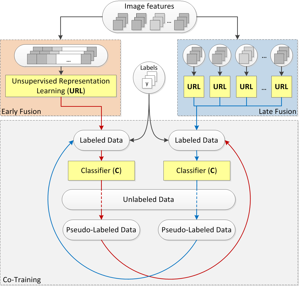
Figure 1: Schema of the proposed strategy.

In standard co-training each classifier is built on a single view, often corresponding to a single feature. However, the combination of multiple features is often required to recognize complex visual concepts [10, 11, 12]. Both the classifiers built by CURL exploit all the available image features in such a way that these concepts can be accurately recognized. We argue that the use of two different fusion schemes together with the non-linear transformation produced by the unsupervised learning procedure, makes the two image representations uncorrelated enough to allow an effective co-training of the classifiers.

The proposed strategy is built on two base components: URL (the unsupervised representation learning) and C (the classifier used in co-training). By changing these two components we can have different embodiments of CURL that can be experimented and evaluated.

To assess the merits of our proposal we conducted several experiments on widely used data sets: the 15-scene data set, the Caltech-101 object classification data set, and the ILSVCR 2012 data set which contains 1000 different classes. We considered a variety of scenarios including transductive learning (i.e. unlabeled test data available during training), inductive learning (i.e. test data not available during training), and self-taught learning (i.e. test and training data coming from two different data sets). In order to verify the efficacy of the CURL classification strategy, we also tested two embodiments: one that uses Ensemble Projection unsupervised representation coupled with Logistic Regression classification, and one based on LapSVM semi-supervised classification. Moreover different variants of the embodiments are evaluated as well. The results show that CURL clearly outperforms other semi-supervised learning methods in the state of the art.

II Related Work

There is a large literature on semi-supervised learning. For the sake of brevity, we discuss only the paradigms involved in the proposed strategy. More information about these and other approaches to semi-supervised learning can be found in the book by Chapelle et al. [1].

II-A Co-training

Blum and Mitchell proposed co-training in 1998 [8] and verified its effectiveness for the classification of web pages. The basic idea is that two classifiers are trained on separate views (features) and then used to train each other. More precisely, when one of the classifiers is very confident in making a prediction for unlabeled data, the predicted labels are used to augment the training set of the other classifier. The concept has been generalized to three [13] or more views [14, 15]. Co-training has been used in several computer vision applications including video annotation [16], action recognition [17], traffic analysis [18], speech and gesture recognition [19], image annotation [20], biometric recognition [21], image retrieval [22], image classification [23], object detection [18, 24], and object tracking [25].

According to Blum and Mitchell, a sufficient condition for the effectiveness of co-training is that, beside being individually accurate, the two classifiers are conditionally independent given the class label. However, conditional independence is not a necessary condition. In fact, Whang and Zhou [26] showed that co-training can be effective when the diversity between the two classifiers is larger than their errors; their results provided a theoretical support to the success of single-view co-training variants [27, 28, 29] (the reader may refer to an updated study from the same authors [30] for more details about necessary and sufficient conditions for co-training).

II-B Unsupervised representation learning

In the last years, as a consequence of the success of deep learning frameworks we observed an increased interest in methods that make use of unlabeled data to automatically learn new representations. In fact, these have been demonstrated to be very effective for the pre-training of large neural networks [31, 32]. Restricted Boltzmann Machines [33] and auto-encoder networks [34] are notable examples of this kind of methods. The tutorial by Bengio covers in detail this family of approaches [35].

A conceptually simpler approach consists in using clustering algorithms to identify frequently occurring patterns in unlabeled data that can be used to define effective representations. The K-means algorithm has been widely used for this purpose [36]. In computer vision this approach is very popular and lead to the many variants of bag-of-visual-words representations [37, 38]. Briefly, clustering on unlabeled data is used to build a vocabulary of visual words. Given an image, multiple local features are extracted and for each of them the most similar visual word is searched. The final representation is a histogram counting the occurrences of the visual words. Sparse coding can be seen as an extension of this approach, where each local feature is described as a sparse combination of multiple words of the vocabulary [39, 40, 41].

Another strategy for unsupervised feature learning is represented by Ensemble Projection (EP) [42]. From all the available data (labeled and unlabeled) Ensemble Projection samples a set of prototypes. Discriminative learning is then used to learn projection functions tuned to the prototypes. Since a single set of projections could be too noisy, multiple sets of prototypes are sampled to build an ensemble of projection functions. The values computed according to these functions represent the components of the learned representations.

LapSVM [7] can be seen as an unsupervised representation learning method as well. In this case the learned representation is not explicit but it is implicitly embedded in a kernel learned from unlabeled data.

II-C Fusion schemes

Combining multimodal information is an important issue in pattern recognition. The fusion of multimodal inputs can bring complementary information from various sources, useful for improving the quality of the image retrieval and classification performance [43]. The problem arises in defining how these modalities are to be combined or fused. In general, the existing fusion approaches can be categorized as early and late fusion approaches, which refers to their relative position from the feature comparison or learning step in the whole processing chain. Early fusion usually refers to the combination of the features into a single representation before comparison/learning. Late fusion refers to the combination, at the last stage, of the responses obtained after individual features comparison or learning [44, 45]. There is no universal conclusion as to which strategy is the preferred method for for a given task. For example, Snoek et al. [44] found that late fusion is better than early fusion in the TRECVID 2004 semantic indexing task, while Ayache et al. [46] stated that early fusion gets better results than late fusion on the TRECVID 2006 semantic indexing task. A combination of these approaches can also be exploited as hybrid fusion approach [47].

Another form of data fusion is Multiple Kernel Learning (MKL). MKL has been introduced by Lanckriet et al. [48] as extension of the support vector machines (SVMs). Instead of using a single kernel computed on the image representation as in standard SVMs, MKL learns distinct kernels. The kernels are combined with a linear or non linear function and the function’s parameters can be determined during the learning process. MKL can be used to learn different kernels on the same image representation or by learning different kernels each one on a different image representation [49]. The former corresponds to have different notion of similarity, and to choose the most suitable one for the problem and representation at hand. The latter corresponds to have multiple representations each with a, possibly, different definition of similarity that must be combined together. This kind of data fusion, in [45], is termed intermediate fusion.

III The Proposed strategy: CURL

In the semi-supervised image classification setup the training data consists of both labeled examples $\{\mathcal{X}_{l},\mathcal{Y}\}=\{({\mathbf{x}}_{i},y_{i})\}_{\scriptscriptstyle i=1}^{\scriptscriptstyle L}$ and unlabeled ones $\mathcal{X}_{u}=\{{\mathbf{x}}_{i}\}_{\scriptscriptstyle i=L+1}^{\scriptscriptstyle L+U}$, where $\mathbf{x}_{i}$ denotes the feature vector of image $i$, $y_{i}\in\{1,\ldots,K\}$ is its label, and $K$ is the number of classes.

In this work, for each image $i$ a set of $S$ different image features $\mathbf{x}_{i}^{(s)}$, $s=1,\ldots,S$ is considered. Two views are then generated by using two different fusion strategies: early and late fusion. In case of Early Fusion (EF), the image features are concatenated and then used to learn a new representation $\mathbf{x}_{i}^{\scriptscriptstyle EF}=\varphi(\{[\mathbf{x}_{i}^{(1)},\ldots,\mathbf{x}_{i}^{(S)}]\}$ in an unsupervised way, where $\varphi(\cdot)$ is a projection function. In case of Late Fusion (LF), an unsupervised representation $\varphi_{s}(\mathbf{x}_{i}^{(s)})$ is independently learned for each image feature and then the representations are concatenated to obtain $\mathbf{x}_{i}^{\scriptscriptstyle LF}=[\varphi_{1}(\mathbf{x}_{i}^{(1)}),\ldots,\varphi_{S}(\mathbf{x}_{i}^{(S)})]$.

Using the learned EF and LF unsupervised representations, the two views are built: $\mathcal{X}_{l}^{\scriptscriptstyle EF}=\{\mathbf{x}_{i}^{\scriptscriptstyle EF}\}_{\scriptscriptstyle i=1}^{\scriptscriptstyle L}$, $\mathcal{X}_{u}^{\scriptscriptstyle EF}=\{\mathbf{x}_{i}^{\scriptscriptstyle EF}\}_{\scriptscriptstyle i=L+1}^{\scriptscriptstyle L+U}$ and $\mathcal{X}_{l}^{\scriptscriptstyle LF}=\{\mathbf{x}_{i}^{\scriptscriptstyle LF}\}_{\scriptscriptstyle i=1}^{\scriptscriptstyle L}$, $\mathcal{X}_{u}^{\scriptscriptstyle LF}=\{\mathbf{x}_{i}^{\scriptscriptstyle LF}\}_{\scriptscriptstyle i=L+1}^{\scriptscriptstyle L+U}$. Furthermore, two label sets $\mathcal{Y}^{\scriptscriptstyle EF}$ and $\mathcal{Y}^{\scriptscriptstyle LF}$ are initialized equal to $\mathcal{Y}$.

Once the two views are generated, our method iteratively co-trains two classifiers $\phi_{\scriptscriptstyle EF}$ and $\phi_{\scriptscriptstyle LF}$ on them [8]. SVMs, logistic regressions, or any other similar technique can be used to obtain them. The idea of iterative co-training is that one can use a small labeled sample to train the initial classifiers over the respective views (i.e. $\phi_{\scriptscriptstyle EF}:\mathcal{X}_{l}^{\scriptscriptstyle EF}\mapsto{\mathcal{Y}}^{\scriptscriptstyle EF}$ and $\phi_{\scriptscriptstyle LF}:\mathcal{X}_{l}^{\scriptscriptstyle LF}\mapsto{\mathcal{Y}}^{\scriptscriptstyle LF}$), and then iteratively bootstrap by taking unlabeled examples for which one of the classifiers is confident but the other is not. The confident classifier determines pseudo-labels [50] that are then used as if they were true labels to improve the other classifier [51]. Given the classifier confidence scores $\mathbf{w}_{i}^{\scriptscriptstyle EF}=\phi_{\scriptscriptstyle EF}(\mathbf{x}_{i}^{\scriptscriptstyle EF})$ and $\mathbf{w}_{i}^{\scriptscriptstyle LF}=\phi_{\scriptscriptstyle LF}(\mathbf{x}_{i}^{\scriptscriptstyle LF})$, the pseudo-labels $\hat{y}_{i}^{\scriptscriptstyle EF}$ and $\hat{y}_{i}^{\scriptscriptstyle LF}$ are respectively obtained as:

$$\hat{y}_{i}^{\scriptscriptstyle EF}={\text{arg}}\!\!\!\max_{j=1,\ldots,K}\mathbf{w}_{i}^{\scriptscriptstyle EF}[j]$$ (1)

$$\hat{y}_{i}^{\scriptscriptstyle LF}={\text{arg}}\!\!\!\max_{j=1,\ldots,K}\mathbf{w}_{i}^{\scriptscriptstyle LF}[j]$$ (2)

In each round of co-training, the classifier $\phi_{\scriptscriptstyle LF}$ chooses some examples in $\mathcal{X}_{u}^{\scriptscriptstyle EF}$ to pseudo-label for $\phi_{\scriptscriptstyle EF}$, and vice versa. For each class $k$, let us call $\mathcal{X}_{\star}$ the set of candidate unlabeled examples to be pseudo-labeled for $\phi_{\scriptscriptstyle EF}$. Each $\mathbf{x}_{\star}\in\mathcal{X}_{\star}$ must belong to the unlabeled set, i.e. $\mathbf{x}_{\star}\in\mathcal{X}_{u}^{\scriptscriptstyle EF}$, has not to be already used for training, i.e. $\mathbf{x}_{\star}\notin\mathcal{X}_{l}^{\scriptscriptstyle EF}$, and its pseudo-label has to be $\hat{y}_{\star}^{\scriptscriptstyle LF}=k$. Furthermore, $\phi_{\scriptscriptstyle LF}$ should be more confident on the classification of $\mathbf{x}_{\star}$ than $\phi_{\scriptscriptstyle EF}$, and its confidence should be higher than a fixed threshold $t_{1}$:

$$\forall\mathbf{x}_{\star}\in\mathcal{X}_{\star}:\mathbf{w}_{\star}^{\scriptscriptstyle EF}[k]<\mathbf{w}_{\star}^{\scriptscriptstyle LF}[k],\mathbf{w}_{\star}^{\scriptscriptstyle LF}[k]>\!t_{1}$$ (3)

If no $\mathbf{x}_{\star}$ satisfying Eq. 3 are found, then the constraints are relaxed:

$$\forall\mathbf{x}_{\star}\in\mathcal{X}_{\star}:\mathbf{w}_{\star}^{\scriptscriptstyle LF}[k]>\!t_{2},\text{ with }t_{2}<t_{1}$$ (4)

Non-maximum suppression is applied to add one single pseudo-labeled example for each class by extracting the most confident $\mathbf{x}_{\star}\in\mathcal{X}_{\star}$:

$$\text{find }\mathbf{x}_{\star}\in\mathcal{X}_{\star}:\mathbf{w}_{\star}^{\scriptscriptstyle LF}[k]=\displaystyle\text{arg}\!\max_{j}\mathbf{w}_{j}^{\scriptscriptstyle LF}[k]$$ (5)

The selected $\mathbf{x}_{\star}$ and its corresponding pseudo-label $\hat{y}_{\star}$ are added to $\mathcal{X}_{l}^{\scriptscriptstyle LF}$ and $\mathcal{Y}^{\scriptscriptstyle LF}$ respectively. If no $\mathbf{x}_{\star}$ satisfying Eq. 4 are found, then nothing is added to $\mathcal{X}_{l}^{\scriptscriptstyle LF}$ and $\mathcal{Y}^{\scriptscriptstyle LF}$.

Similarly, the classifier $\phi_{\scriptscriptstyle EF}$ chooses some examples in $\mathcal{X}_{u}^{\scriptscriptstyle LF}$ to pseudo-label for $\phi_{\scriptscriptstyle LF}$. At the next co-training round, two new classifiers $\phi_{\scriptscriptstyle EF}$ and $\phi_{\scriptscriptstyle LF}$ are trained on the respective views, that now contain both labeled and pseudo-labeled examples. The complete procedure of the CURL method is outlined in Algorithms 1-3.

Data: Labeled data $\{\mathcal{X}_{l},\mathcal{Y}\}$, unlabeled data $\mathcal{X}_{u}$

Result: Classifiers $\phi_{\scriptscriptstyle EF}(\cdot)$ and $\phi_{\scriptscriptstyle LF}(\cdot)$

begin

       $[\mathcal{X}_{l}^{\scriptscriptstyle EF}\!,\!\mathcal{X}_{u}^{\scriptscriptstyle EF}\!,\!\mathcal{X}_{l}^{\scriptscriptstyle LF}\!,\!\mathcal{X}_{u}^{\scriptscriptstyle LF}]=\text{\bf{computeURL}}(\mathcal{X}_{l},\mathcal{X}_{u})$

       ${\mathcal{Y}}^{\scriptscriptstyle EF}={\mathcal{Y}}^{\scriptscriptstyle LF}={\mathcal{Y}}$

       train classifier $\phi_{\scriptscriptstyle EF}:\mathcal{X}_{l}^{\scriptscriptstyle EF}\mapsto{\mathcal{Y}}^{\scriptscriptstyle EF}$

       train classifier $\phi_{\scriptscriptstyle LF}:\mathcal{X}_{l}^{\scriptscriptstyle LF}\mapsto{\mathcal{Y}}^{\scriptscriptstyle LF}$

       for co-training round $c=1:C$ do

             initialize $\mathcal{W}^{\scriptscriptstyle EF}=\mathcal{W}^{\scriptscriptstyle LF}=\hat{\mathcal{Y}}^{\scriptscriptstyle EF}=\hat{\mathcal{Y}}^{\scriptscriptstyle LF}=\emptyset$

            

            foreach $\mathbf{x}_{i}^{\scriptscriptstyle EF}\in\mathcal{X}_{u}^{\scriptscriptstyle EF}$ do

                   add $\mathbf{w}_{i}^{\scriptscriptstyle EF}=\phi_{\scriptscriptstyle EF}(\mathbf{x}_{i}^{\scriptscriptstyle EF})$ to $\mathcal{W}^{\scriptscriptstyle EF}$

                   add $\displaystyle\hat{y}_{i}^{\scriptscriptstyle EF}={\text{arg}}\!\!\!\max_{j=1,\ldots,K}\mathbf{w}_{i}^{\scriptscriptstyle EF}[j]$ to $\hat{\mathcal{Y}}^{\scriptscriptstyle EF}$

                  

            foreach $\mathbf{x}_{i}^{\scriptscriptstyle LF}\in\mathcal{X}_{u}^{\scriptscriptstyle LF}$ do

                   add $\mathbf{w}_{i}^{\scriptscriptstyle LF}=\phi_{\scriptscriptstyle LF}(\mathbf{x}_{i}^{\scriptscriptstyle LF})$ to $\mathcal{W}^{\scriptscriptstyle LF}$

                   add $\displaystyle\hat{y}_{i}^{\scriptscriptstyle LF}={\text{arg}}\!\!\!\max_{j=1,\ldots,K}\mathbf{w}_{i}^{\scriptscriptstyle LF}[j]$ to $\hat{\mathcal{Y}}^{\scriptscriptstyle LF}$

                  

            

            for class number $k=1:K$ do

                  

                  for $(v_{1},v_{2})\in\{(\text{\footnotesize{EF},\footnotesize{LF}}),(\text{\footnotesize{LF},\footnotesize{EF}})\}$ do

                        

                        find $\{\mathcal{X}_{\star},\hat{\mathcal{Y}}_{\star}^{v_{2}}\}$ with

                         $\mathcal{X}_{\star}\!\subset\!\mathcal{X}_{u}^{v_{1}}$, $\mathcal{X}_{\star}\!\cap\!\mathcal{X}_{l}^{v_{1}}\!=\!\emptyset$, $\hat{\mathcal{Y}}_{\star}^{v_{2}}\subset\hat{\mathcal{Y}}^{v_{2}}$ s.t.:

                         $\forall\mathbf{x}_{\star}\!\in\!\mathcal{X}_{\star}$ and $\forall\hat{y}_{\star}^{v_{2}}\!\in\!\hat{\mathcal{Y}}_{\star}^{v_{2}}$, hold:

                         $\hat{y}_{\star}^{v_{2}}=k,\mathbf{w}_{\star}^{v_{1}}[k]<\mathbf{w}_{\star}^{v_{2}}[k],\mathbf{w}_{\star}^{v_{2}}[k]>\!t_{1}$

                         if $\mathcal{X}_{\star}=\emptyset$ then

                               find $\{\mathcal{X}_{\star},\hat{\mathcal{Y}}_{\star}^{v_{2}}\}$ with

                               $\mathcal{X}_{\star}\!\subset\!\mathcal{X}_{u}^{v_{1}}$, $\mathcal{X}_{\star}\!\cap\!\mathcal{X}_{l}^{v_{1}}\!=\!\emptyset$, $\hat{\mathcal{Y}}_{\star}^{v_{2}}\!\subset\!\hat{\mathcal{Y}}^{v_{2}}$ s.t.:

                               $\forall\mathbf{x}_{\star}\!\in\!\mathcal{X}_{\star}$ and $\forall\hat{y}_{\star}^{v_{2}}\!\in\!\hat{\mathcal{Y}}_{\star}^{v_{2}}$, hold:

                               $\hat{y}_{\star}^{v_{2}}=k$, $\mathbf{w}_{\star}^{v_{2}}[k]>t_{2}$

                              

                        

                        $[\mathcal{X}_{\star},\!\hat{\mathcal{Y}}_{\star}^{v_{2}}\!]\!=\!\text{\bf{nonMaxSuppr}}(\!\mathcal{X}_{\star},\!\hat{\mathcal{Y}}_{\star}^{v_{2}},\!\mathcal{W}^{v_{2}}\!)$

                         $\mathcal{X}_{l}^{v_{1}}=\mathcal{X}_{l}^{v_{1}}\cup{\mathcal{X}}_{\star}$

                         $\mathcal{Y}^{v_{1}}=\mathcal{Y}^{v_{1}}\cup\hat{\mathcal{Y}}_{\star}^{v_{2}}$

                        

                  

            

            train classifier $\phi_{\scriptscriptstyle EF}:\mathcal{X}_{l}^{\scriptscriptstyle EF}\mapsto{\mathcal{Y}}^{\scriptscriptstyle EF}$

             train classifier $\phi_{\scriptscriptstyle LF}:\mathcal{X}_{l}^{\scriptscriptstyle LF}\mapsto{\mathcal{Y}}^{\scriptscriptstyle LF}$

            

      

Algorithm 1 CURL

Data: Labeled data $\mathcal{X}_{l}$ and unlabeled data $\mathcal{X}_{u}$

Result: Unsup. representations $\mathcal{X}_{l}^{EF},\mathcal{X}_{u}^{EF},\mathcal{X}_{l}^{LF},\mathcal{X}_{u}^{LF}$

begin

      

      Learn EF representation $\varphi$ on $\{[\mathbf{x}_{i}^{(1)},\ldots,\mathbf{x}_{i}^{(S)}]\}_{i=1}^{L+U}$

       $\mathcal{X}_{l}^{\scriptscriptstyle EF}=\varphi(\{[\mathbf{x}_{i}^{(1)},\ldots,\mathbf{x}_{i}^{(S)}]\}_{i=1}^{L})$

       $\mathcal{X}_{u}^{\scriptscriptstyle EF}=\varphi(\{[\mathbf{x}_{i}^{(1)},\ldots,\mathbf{x}_{i}^{(S)}]\}_{i=L+1}^{L+U})$

       Learn LF representations $\varphi_{s}$ on $\{\mathbf{x}_{i}^{(s)}\}_{i=1}^{L+U}$ $\mathcal{X}_{l}^{\scriptscriptstyle LF}=\{[\varphi_{1}(\mathbf{x}_{i}^{(1)}),\ldots,\varphi_{S}(\mathbf{x}_{i}^{(S)})]\}_{i=1}^{L}$

       $\mathcal{X}_{u}^{\scriptscriptstyle LF}=\{[\varphi_{1}(\mathbf{x}_{i}^{(1)}),\ldots,\varphi_{S}(\mathbf{x}_{i}^{(S)})]\}_{i=L+1}^{L+U}$

      

Algorithm 2 compute URL

Data: $\mathcal{X},\hat{\mathcal{Y}},\mathcal{W},k$

Result: $\mathcal{X}_{\star},\hat{\mathcal{Y}}_{\star}$

begin

       find $\{\mathcal{X}_{\star},\hat{\mathcal{Y}}_{\star}\}$ with $\mathcal{X}_{\star}\in\mathcal{X}$, $\hat{\mathcal{Y}}_{\star}\in\hat{\mathcal{Y}}$ s.t.:

       $\quad\mathbf{w}_{\star}[k]=\displaystyle\text{arg}\!\max_{j}\mathbf{w}_{j}[k]$, with $\mathbf{w}_{j}\in\mathcal{W}$

      

Algorithm 3 non-maximum suppression

IV Experiments

CURL is parametric with respect to the projection function $\varphi$ used in the unsupervised representation learning URL, and the supervised classification technique C used during to co-train $\phi_{\scriptscriptstyle EF}$ and $\phi_{\scriptscriptstyle LF}$. As first embodiment of CURL, we used Ensemble Projection [42] for the former and logistic regression for the latter. Another embodiment, based on LapSVM [7] is presented in Section V-C.

IV-A Data sets

We evaluated our method on two data sets: Scene-15 (S-15) [38], and Caltech-101 (C-101) [52]. Scene-15 data set contains 4485 images divided into 15 scene categories with both indoor and outdoor environments. Each category has 200 to 400 images. Caltech-101 contains 8677 images divided into 101 object categories, each having 31 to 800 images. Furthermore, we collected a set of random images by sampling 20,000 images from the ImageNet data set [53] to evaluate our method on the task of self-taught image classification. Since the current version of ImageNet has 21841 synsets (i.e. categories) and a total of more than 14 millions images, there is a small probability that the random images and images in the two considered data sets come from the same distribution.

IV-B Image features

In our experiments we used the following three features: GIST [54], Pyramid of Histogram of Oriented Gradients (PHOG) [55], and Local Binary Patterns (LBP) [56]. GIST was computed on the rescaled images of 256$\times$256 pixels, at 3 scales with 4, 8 and 8 orientations respectively. PHOG was computed with a 2-layer pyramid and in 8 directions. Uniform LBP with radius equal to 1, and 8 neighbors was used.

In Section V-B we also investigate the use of features extracted from a CNN [57] in combination with the previous ones.

IV-C Ensemble projection

Differently from others semi-supervised methods that train a classifier from labeled data with a regularization term learned from unlabeled data, Ensemble Projection [42] learns a new image representation from all known data (i.e. labeled and unlabeled data), and then trains a plain classifier on it.

Ensemble Projection learns knowledge from $T$ different prototype sets $\mathcal{P}^{t}=\{(s_{i}^{t},c_{i}^{t})\}_{i=1}^{rn}$, with $t\in\{1,\ldots,T\}$ where $s_{i}^{t}\in\{1,\ldots,L+U\}$ is the index of the $i-$th chosen image, $c_{i}^{t}\in\{1,\ldots,r\}$ is the pseudo-label indicating to which prototype $s_{i}^{t}$ belong to. $r$ is the number of prototypes in $\mathcal{P}^{t}$, and $n$ is the number of images sampled for each prototype. For each prototype set, $m$ hypotheses are randomly sampled, and the one containing images having the largest mutual distance is kept.

A set of discriminative classifiers $\phi^{t}(\cdot)$ is learned on $\mathcal{P}^{t}$, one for each prototype set, and the projected vectors $\phi^{t}(\mathbf{x}_{i})$ are obtained. The final feature vector is obtained by concatenating these projected vectors.

Following [42] we set $T=300$, $r=30$, $n=6$, $m=50$, using Logistic Regression (LR) as discriminative classifier $\phi^{t}(\cdot)$ with $C=15$.

Within CURL, Ensemble Projection is used to learn both Early Fusion and Late Fusion unsupervised representations. In the case of Early Fusion (EF), the feature vector $\mathbf{x}_{i}$ is obtained concatenating the $S$ different features available $\mathbf{x}_{i}=[\mathbf{x}_{i}^{(1)},\ldots,\mathbf{x}_{i}^{(S)}]$, $s=1,\ldots,S$. In the case of Late Fusion (LF), the feature vector $\mathbf{x}_{i}$ is made by considering just one single feature at time $\mathbf{x}_{i}=\mathbf{x}_{i}^{(s)}$. For both EF and LF, the same number $T$ of prototypes is used in order to assure that the unsupervised representations have the same size.

IV-D Experimental settings

We conducted two kinds of experiments: (1) comparison of our strategy with competing methods for semi-supervised image classification; (2) evaluation of our method at different number of co-training rounds. We considered three scenarios corresponding to three different ways of using unlabeled data. In the inductive learning scenario 25% of the unlabeled data is used together with the labeled data for the semi-supervised training of the classifier; the remaining 75% is used as an independent test set. In the transductive learning scenario all the unlabeled data is used during both training and test. In the self-taught learning scenario the set of unlabeled data is taken from an additional data set featuring a different distribution of image content (i.e. the 20,000 images from ImageNet); all the unlabeled data from the original data set is used as an independent test set.

As evaluation measure we followed [42] and used the multi-class average precision (MAP), computed as the average precision over all recall values and over all classes. Different numbers of training images per class were tested for both Scene-15 and Caltech-101 (i.e. 1, 2, 3, 5, 10, and 20). All the reported results represent the average performance over ten runs with random labeled-unlabeled splits.

The performance of the proposed strategy are compared with those of other supervised and semi-supervised baseline methods. As supervised classifiers we considered Support Vector Machines (SVM). As semi-supervised classifiers, we used LapSVM [58, 7]. LapSVM extend the SVM framework including a smoothness penalty term defined on the Laplacian adjacency graph built from both labeled and unlabeled data. For both SVM and LapSVM we experimented with the linear, RBF and $\chi^{2}$ kernels computed on the concatenation of the three available image features as in [42]. The parameters of SVM and LapSVM have been determined by a greedy search with a three-fold cross validation on the training set. We also compared the present embodiment of CURL against Ensemble Projection coupled with a logistic regression classifier (EP+LR) as in [42].

V Experimental results

As a first experiment we compared CURL against EP+LR, and against SVMs and LapSVMs with different kernels. Specifically, we tested the two co-trained classifiers operating on early-fused and late-fused representations, both employing EP for URL and LR as classifier C, that we call CURL-EF(EP+LR) and CURL-LF(EP+LR) respectively. We also included a variant of the proposed method. It differs in the number of pseudo-labeled examples that are added at each co-training round. The variant skips the non-maximum suppression step, and at each round, adds all the examples satisfying Eq. 3. We denote the two co-trained classifiers of the variant as CURL-EF_n(EP+LR) and CURL-LF_n(EP+LR).

Fig. 2 shows the classification performance with different numbers of labeled training images per class, in the three learning scenarios for both the Scene-15 and Caltech-101 data sets. For the CURL-based methods we considered five co-training rounds, and the reported performance correspond to the last round. For SVM and LapSVM only the results using $\chi^{2}$ kernel are reported, since they consistently showed the best performance across all the experiments.

Scene-15 inductive	Scene-15 transductive	Scene-15 self-taught
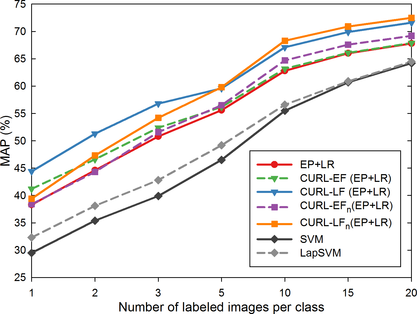
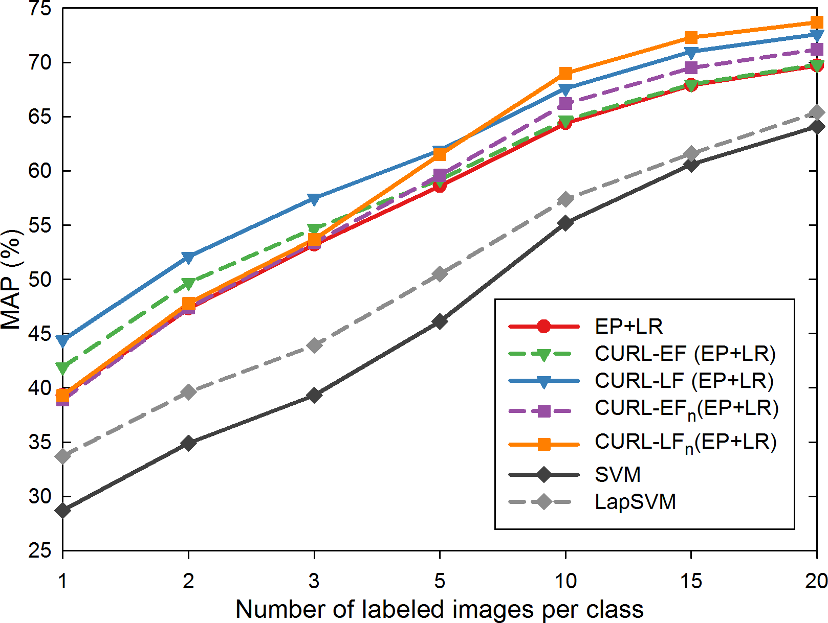
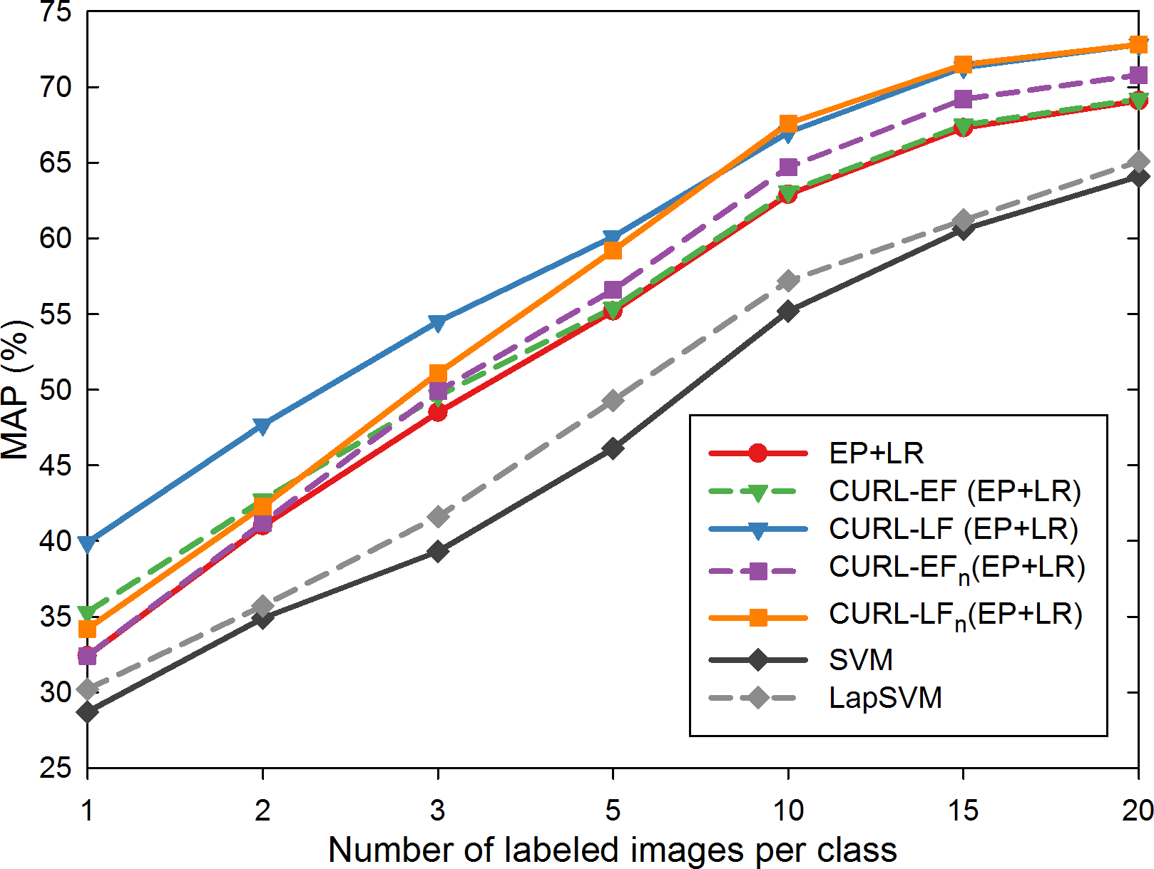
Caltech-101 inductive	Caltech-101 transductive	Caltech-101 self-taught

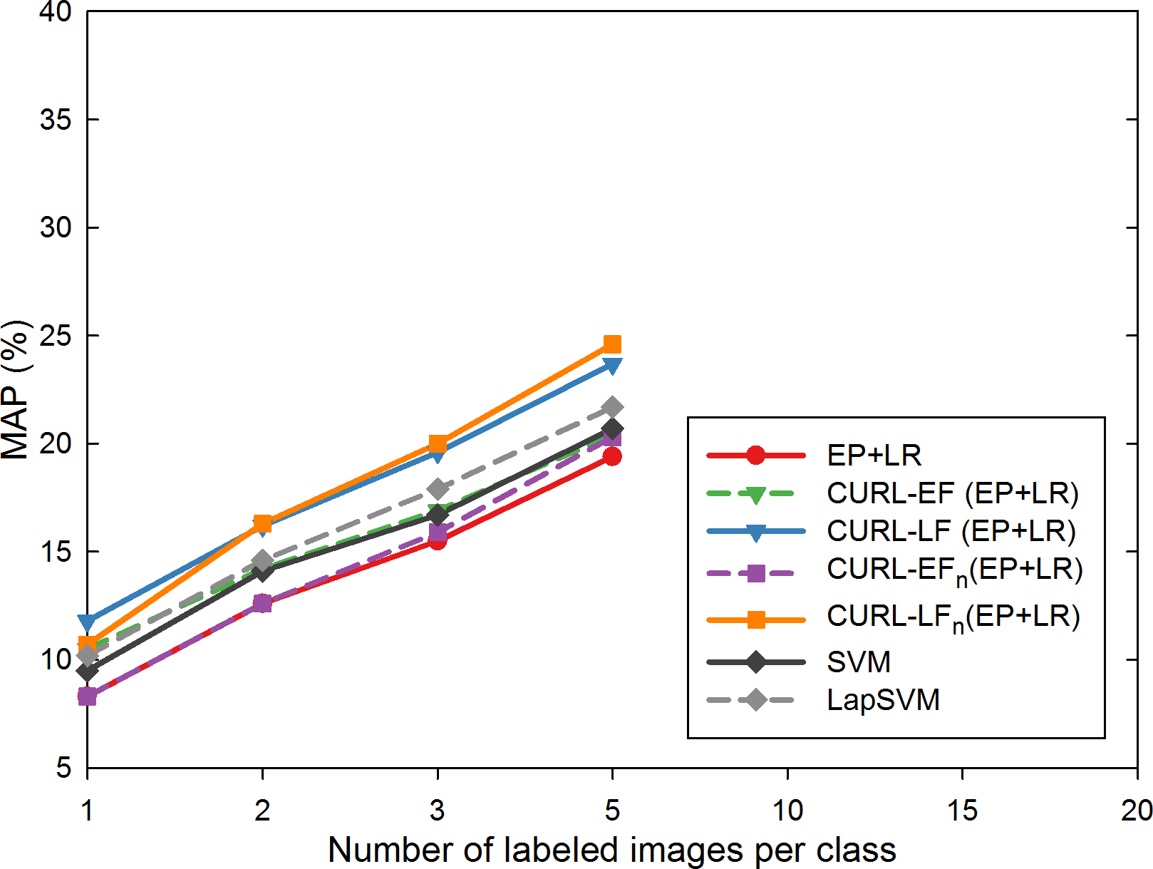
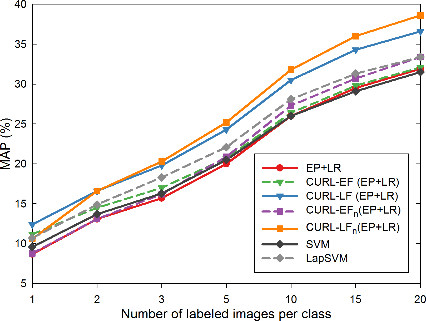
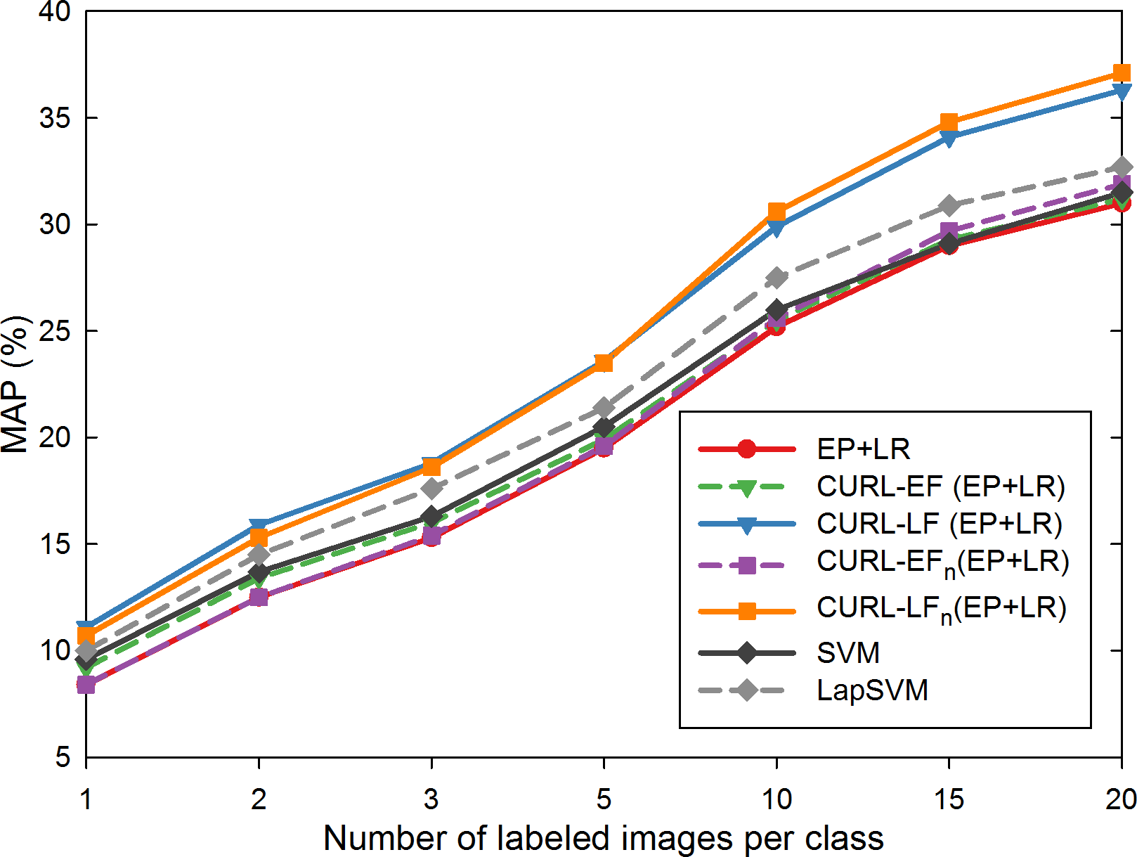
Figure 2: Mean Average Precision (MAP) varying the number of labeled images per class, obtained on the Scene-15 data set (first row), and on the Caltech-101 data set (second row). Three scenarios are considered: inductive learning (left column), transductive learning (middle column) and self-taught learning (third column). Note that inductive learning on the Caltech-101 data set is limited to 5 labeled images per class because otherwise for some classes there wouldn’t be enough unlabeled data left for both training and evaluation.

Detailed results for all the tested baseline methods, and for the CURL variants across the co-training rounds are available in Tables I, II and III.

TABLE I: Mean Average Precision (MAP) of the baseline algorithms, varying the number of labeled images per class in the three learning scenarios considered: inductive (IND), transductive (TRD), and self-taught (ST).

Scene-15 # img method IND TRD ST 1 SVMlin 22.7 22.3 22.3 SVMrbf 26.5 25.8 25.8 SVM${}_{\chi^{2}}$ 29.5 28.7 28.7 LapSVMlin 28.1 29.1 26.4 LapSVMrbf 28.8 29.8 26.7 LapSVM${}_{\chi^{2}}$ 32.3 33.7 30.2 EP+LR 38.3 39.3 32.4 2 SVMlin 27.4 26.9 26.9 SVMrbf 32.9 31.3 31.3 SVM${}_{\chi^{2}}$ 35.4 34.9 34.9 LapSVMlin 33.7 34.9 31.2 LapSVMrbf 34.6 35.7 32.5 LapSVM${}_{\chi^{2}}$ 38.1 39.6 35.7 EP+LR 44.6 47.3 41.0 3 SVMlin 30.0 30.2 30.2 SVMrbf 36.5 36.7 36.7 SVM${}_{\chi^{2}}$ 39.9 39.3 39.3 LapSVMlin 37.6 38.6 36.4 LapSVMrbf 37.7 38.9 37.2 LapSVM${}_{\chi^{2}}$ 42.8 43.9 41.6 EP+LR 50.8 53.2 48.5 5 SVMlin 35.5 35.2 35.2 SVMrbf 43.5 42.8 42.8 SVM${}_{\chi^{2}}$ 46.5 46.1 46.1 LapSVMlin 43.4 44.5 43.5 LapSVMrbf 43.8 44.7 44.0 LapSVM${}_{\chi^{2}}$ 49.2 50.5 49.3 EP+LR 55.6 58.6 55.2 10 SVMlin 43.8 43.7 43.7 SVMrbf 51.9 51.3 51.3 SVM${}_{\chi^{2}}$ 55.5 55.2 55.2 LapSVMlin 51.4 52.5 52.3 LapSVMrbf 52.4 53.1 53.0 LapSVM${}_{\chi^{2}}$ 56.6 57.4 57.2 EP+LR 62.8 64.4 62.9 15 SVMlin 50.1 50.3 50.3 SVMrbf 57.4 57.1 57.1 SVM${}_{\chi^{2}}$ 60.7 60.6 60.6 LapSVMlin 55.1 56.0 55.5 LapSVMrbf 57.8 58.7 58.3 LapSVM${}_{\chi^{2}}$ 60.9 61.6 61.2 EP+LR 66.0 67.9 67.3 20 SVMlin 54.0 53.5 53.5 SVMrbf 60.4 60.3 60.3 SVM${}_{\chi^{2}}$ 64.2 64.1 64.1 LapSVMlin 58.3 58.7 58.6 LapSVMrbf 60.8 61.4 61.2 LapSVM${}_{\chi^{2}}$ 64.5 65.4 65.1 EP+LR 67.8 69.7 69.1

Caltech-101 # img method IND TRD ST 1 SVMlin 6.0 6.3 6.3 SVMrbf 7.1 7.3 7.3 SVM${}_{\chi^{2}}$ 9.5 9.6 9.6 LapSVMlin 9.2 9.6 9.1 LapSVMrbf 9.8 10.2 9.6 LapSVM${}_{\chi^{2}}$ 10.2 10.7 10.0 EP+LR 8.3 8.7 8.4 2 SVMlin 9.1 9.2 9.2 SVMrbf 10.1 9.8 9.8 SVM${}_{\chi^{2}}$ 14.1 13.7 13.7 LapSVMlin 12.3 12.8 12.1 LapSVMrbf 12.7 13.3 12.4 LapSVM${}_{\chi^{2}}$ 14.6 14.9 14.5 EP+LR 12.6 13.1 12.5 3 SVMlin 10.7 10.8 10.8 SVMrbf 11.7 11.6 11.6 SVM${}_{\chi^{2}}$ 16.7 16.3 16.3 LapSVMlin 13.8 14.3 13.5 LapSVMrbf 14.0 14.6 13.9 LapSVM${}_{\chi^{2}}$ 17.9 18.3 17.6 EP+LR 15.5 15.7 15.3 5 SVMlin 13.4 13.3 13.3 SVMrbf 14.9 14.6 14.6 SVM${}_{\chi^{2}}$ 20.7 20.5 20.5 LapSVMlin 16.3 16.6 16.0 LapSVMrbf 16.8 17.1 16.6 LapSVM${}_{\chi^{2}}$ 21.7 22.1 21.4 EP+LR 19.4 20.0 19.5 10 SVMlin - 17.3 17.3 SVMrbf - 19.2 19.2 SVM${}_{\chi^{2}}$ - 26.0 26.0 LapSVMlin - 20.5 20.1 LapSVMrbf - 21.6 21.2 LapSVM${}_{\chi^{2}}$ - 28.1 27.5 EP+LR - 26.0 25.2 15 SVMlin - 19.7 19.7 SVMrbf - 22.1 22.1 SVM${}_{\chi^{2}}$ - 29.1 29.1 LapSVMlin - 22.9 22.5 LapSVMrbf - 24.0 23.5 LapSVM${}_{\chi^{2}}$ - 31.3 30.9 EP+LR - 29.5 29.0 20 SVMlin - 21.5 21.5 SVMrbf - 24.2 24.2 SVM${}_{\chi^{2}}$ - 31.5 31.5 LapSVMlin - 24.6 24.0 LapSVMrbf - 26.8 26.1 LapSVM${}_{\chi^{2}}$ - 33.4 32.7 EP+LR - 31.9 31.0

TABLE II: Mean Average Precision (MAP) of the CURL variants, in the (EP+LR) embodiment, varying the number of labeled images per class at the different co-training rounds obtained on the Scene-15 data set in the three learning scenarios considered: inductive (left), transductive (middle), and self-taught (right). For clarity, the (EP+LR) suffixes have been omitted.

# co-train round # img method 0 1 2 3 4 5 1 CURL-EF 38.3 41.0 41.1 41.1 41.1 41.2 CURL-LF 40.0 42.4 43.8 44.0 44.3 44.4 CURL-EF&LF - 43.3 43.7 43.8 44.0 44.0 CURL-EFn 38.3 38.4 38.5 38.4 38.3 38.2 CURL-LFn 40.0 39.9 39.9 39.7 39.6 39.4 CURL-EF&LFn - 40.4 40.4 40.3 40.1 40.0 2 CURL-EF 44.6 46.3 46.4 46.5 46.6 46.6 CURL-LF 48.5 50.2 50.7 50.9 51.1 51.3 CURL-EF&LF - 49.7 50.0 50.1 50.2 50.3 CURL-EFn 44.6 44.3 44.7 44.7 44.5 44.2 CURL-LFn 48.5 48.8 48.8 48.4 48.0 47.3 CURL-EF&LFn - 48.0 48.0 47.8 47.4 46.9 3 CURL-EF 50.8 52.1 52.2 52.3 52.4 52.4 CURL-LF 54.1 55.2 56.2 56.4 56.6 56.8 CURL-EF&LF - 55.3 55.7 55.9 56.0 56.1 CURL-EFn 50.8 51.6 52.5 52.6 52.0 51.8 CURL-LFn 54.1 55.3 55.3 55.1 54.7 54.2 CURL-EF&LFn - 55.0 55.2 55.0 54.4 54.0 5 CURL-EF 55.6 56.1 56.2 56.2 56.2 56.2 CURL-LF 58.3 59.0 59.3 59.5 59.5 59.6 CURL-EF&LF - 59.0 59.1 59.2 59.3 59.4 CURL-EFn 55.6 56.5 57.7 57.7 57.7 57.6 CURL-LFn 58.3 59.7 59.8 60.0 59.8 59.8 CURL-EF&LFn - 59.6 59.9 59.9 59.7 59.6 10 CURL-EF 62.8 63.1 63.2 63.2 63.2 63.2 CURL-LF 66.2 66.5 66.6 66.9 67.0 67.1 CURL-EF&LF - 66.3 66.4 66.5 66.6 66.7 CURL-EFn 62.8 64.7 65.3 65.5 65.8 65.8 CURL-LFn 66.2 67.6 67.8 68.2 68.2 68.3 CURL-EF&LFn - 67.5 67.8 68.0 68.0 68.0 15 CURL-EF 66.0 66.1 66.1 66.1 66.1 66.1 CURL-LF 69.2 69.4 69.6 69.8 69.8 69.9 CURL-EF&LF - 69.3 69.3 69.4 69.4 69.5 CURL-EFn 66.0 67.6 68.3 68.5 68.7 68.8 CURL-LFn 69.2 70.6 70.9 71.0 71.0 70.9 CURL-EF&LFn - 70.4 70.8 70.8 70.9 70.9 20 CURL-EF 67.8 67.9 67.9 67.9 67.9 67.9 CURL-LF 71.1 71.3 71.3 71.5 71.5 71.6 CURL-EF&LF - 71.2 71.2 71.2 71.2 71.3 CURL-EFn 67.8 69.2 69.8 70.1 70.2 70.3 CURL-LFn 71.1 72.0 72.4 72.5 72.5 72.5 CURL-EF&LFn - 71.9 72.2 72.4 72.4 72.4

# co-train round # img method 0 1 2 3 4 5 1 CURL-EF 39.3 41.7 41.9 41.9 41.9 41.9 CURL-LF 39.8 42.6 43.8 44.1 44.2 44.4 CURL-EF&LF - 43.5 43.9 44.1 44.1 44.2 CURL-EFn 39.3 38.9 38.9 38.9 38.7 38.7 CURL-LFn 39.8 39.9 39.9 39.7 39.6 39.3 CURL-EF&LFn - 40.4 40.4 40.4 40.2 40.0 2 CURL-EF 47.3 49.2 49.5 49.6 49.7 49.7 CURL-LF 48.7 50.6 51.5 51.9 52.0 52.1 CURL-EF&LF - 51.2 51.7 51.9 52.0 52.1 CURL-EFn 47.3 47.4 47.8 47.5 47.1 46.9 CURL-LFn 48.7 49.3 49.0 48.8 48.5 47.8 CURL-EF&LFn - 49.6 49.5 49.2 48.8 48.2 3 CURL-EF 53.2 54.4 54.5 54.6 54.7 54.7 CURL-LF 54.8 55.8 56.6 57.2 57.4 57.5 CURL-EF&LF - 56.4 56.8 57.2 57.3 57.4 CURL-EFn 53.2 53.4 53.7 53.5 52.7 52.2 CURL-LFn 54.8 55.4 55.4 54.9 54.4 53.7 CURL-EF&LFn - 55.8 55.7 55.2 54.5 53.9 5 CURL-EF 58.6 59.1 59.2 59.2 59.2 59.2 CURL-LF 60.3 61.3 61.6 61.7 61.9 61.9 CURL-EF&LF - 61.5 61.6 61.7 61.8 61.8 CURL-EFn 58.6 59.6 60.4 60.3 60.0 59.7 CURL-LFn 60.3 61.8 62.0 61.9 61.7 61.5 CURL-EF&LFn - 61.9 62.1 61.9 61.6 61.3 10 CURL-EF 64.4 64.6 64.6 64.6 64.7 64.7 CURL-LF 66.6 67.0 67.2 67.3 67.5 67.6 CURL-EF&LF - 67.1 67.1 67.2 67.3 67.4 CURL-EFn 64.4 66.2 67.0 67.3 67.4 67.5 CURL-LFn 66.6 68.5 68.8 69.0 69.0 69.0 CURL-EF&LFn - 68.4 68.8 69.0 69.0 69.0 15 CURL-EF 67.9 68.0 68.0 68.0 68.0 68.0 CURL-LF 70.1 70.5 70.6 70.7 70.8 71.0 CURL-EF&LF - 70.5 70.6 70.6 70.7 70.8 CURL-EFn 67.9 69.5 70.4 70.7 70.8 70.9 CURL-LFn 70.1 71.7 71.9 72.2 72.3 72.3 CURL-EF&LFn - 71.7 72.1 72.3 72.4 72.4 20 CURL-EF 69.7 69.8 69.8 69.8 69.8 69.8 CURL-LF 72.1 72.2 72.3 72.4 72.5 72.6 CURL-EF&LF - 72.3 72.3 72.4 72.4 72.4 CURL-EFn 69.7 71.2 71.7 72.1 72.2 72.3 CURL-LFn 72.1 73.3 73.6 73.7 73.7 73.7 CURL-EF&LFn - 73.3 73.6 73.7 73.8 73.8

# co-train round # img method 0 1 2 3 4 5 1 CURL-EF 32.4 34.8 35.2 35.3 35.3 35.3 CURL-LF 36.7 38.6 39.6 39.7 39.8 39.9 CURL-EF&LF - 38.4 38.9 38.9 39.0 39.0 CURL-EFn 32.4 32.4 32.8 32.8 32.8 32.3 CURL-LFn 36.7 34.9 34.8 34.8 34.6 34.2 CURL-EF&LFn - 35.5 35.5 35.6 35.4 35.0 2 CURL-EF 41.0 42.4 42.5 42.6 42.6 42.7 CURL-LF 45.4 47.1 47.6 47.5 47.7 47.7 CURL-EF&LF - 46.4 46.5 46.6 46.7 46.7 CURL-EFn 41.0 41.2 42.7 42.5 41.6 41.4 CURL-LFn 45.4 44.3 44.2 43.7 43.1 42.3 CURL-EF&LFn - 44.8 45.1 44.7 43.7 43.0 3 CURL-EF 48.5 49.4 49.5 49.5 49.5 49.6 CURL-LF 53.4 54.0 54.5 54.4 54.5 54.5 CURL-EF&LF - 53.5 53.6 53.6 53.6 53.6 CURL-EFn 48.5 49.9 50.6 50.6 49.8 49.3 CURL-LFn 53.4 52.0 52.3 52.0 51.6 51.1 CURL-EF&LFn - 52.8 52.9 52.6 51.9 51.3 5 CURL-EF 55.2 55.4 55.5 55.5 55.5 55.4 CURL-LF 59.4 59.8 60.0 60.1 60.1 60.1 CURL-EF&LF - 59.3 59.4 59.4 59.4 59.4 CURL-EFn 55.2 56.6 57.5 57.5 57.2 57.1 CURL-LFn 59.4 59.5 59.6 59.6 59.4 59.2 CURL-EF&LFn - 59.8 59.8 59.7 59.3 59.1 10 CURL-EF 62.9 63.1 63.1 63.1 63.1 63.1 CURL-LF 66.0 66.4 66.7 66.7 66.9 67.0 CURL-EF&LF - 66.6 66.7 66.7 66.7 66.8 CURL-EFn 62.9 64.7 65.7 66.0 66.1 66.3 CURL-LFn 66.0 67.1 67.3 67.5 67.6 67.6 CURL-EF&LFn - 67.2 67.6 67.7 67.8 67.8 15 CURL-EF 67.3 67.5 67.5 67.5 67.5 67.5 CURL-LF 70.5 70.8 70.9 71.1 71.2 71.3 CURL-EF&LF - 71.0 71.0 71.1 71.2 71.2 CURL-EFn 67.3 69.2 69.8 70.1 70.2 70.2 CURL-LFn 70.5 70.8 71.1 71.3 71.5 71.5 CURL-EF&LFn - 71.3 71.5 71.7 71.8 71.8 20 CURL-EF 69.1 69.2 69.2 69.2 69.2 69.2 CURL-LF 72.3 72.4 72.4 72.5 72.6 72.8 CURL-EF&LF - 72.6 72.6 72.7 72.7 72.8 CURL-EFn 69.1 70.8 71.5 71.7 71.8 71.9 CURL-LFn 72.3 72.4 72.7 72.8 72.8 72.8 CURL-EF&LFn - 72.9 73.2 73.2 73.3 73.3

TABLE III: Mean Average Precision (MAP) of the CURL variants, in the (EP+LR) embodiment, varying the number of labeled images per class at the different co-training rounds obtained on the Caltech-101 data set in the three learning scenarios considered: inductive (left), transductive (middle), and self-taught (right). For clarity, the (EP+LR) suffixes have been omitted.

# co-train round # img method 0 1 2 3 4 5 1 CURL-EF 8.3 10.4 10.5 10.5 10.5 10.5 CURL-LF 10.1 11.6 11.8 11.8 11.8 11.8 CURL-EF&LF - 11.5 11.6 11.6 11.6 11.6 CURL-EFn 8.3 8.3 8.5 8.5 8.8 8.8 CURL-LFn 10.1 10.3 10.3 10.6 10.7 10.7 CURL-EF&LFn - 9.5 9.6 9.8 10.0 10.1 2 CURL-EF 12.6 14.2 14.3 14.3 14.3 14.2 CURL-LF 15.3 16.3 16.3 16.3 16.2 16.2 CURL-EF&LF - 15.9 15.9 15.8 15.8 15.8 CURL-EFn 12.6 12.6 13.4 13.5 13.9 14.1 CURL-LFn 15.3 15.7 15.9 16.1 16.2 16.3 CURL-EF&LFn - 14.6 15.1 15.3 15.5 15.7 3 CURL-EF 15.5 16.8 16.9 16.8 16.9 16.9 CURL-LF 18.8 19.4 19.6 19.6 19.7 19.6 CURL-EF&LF - 18.9 19.0 18.9 18.9 18.9 CURL-EFn 15.5 15.9 16.8 16.9 17.1 17.1 CURL-LFn 18.8 19.5 19.8 20.0 20.0 20.0 CURL-EF&LFn - 18.5 19.0 19.2 19.3 19.2 5 CURL-EF 19.4 20.2 20.4 20.4 20.4 20.4 CURL-LF 23.2 23.4 23.7 23.7 23.7 23.7 CURL-EF&LF - 22.9 23.0 23.0 23.0 23.0 CURL-EFn 19.4 20.3 21.0 21.2 21.3 21.3 CURL-LFn 23.2 24.2 24.4 24.6 24.6 24.6 CURL-EF&LFn - 23.3 23.7 23.9 23.9 24.0 10 CURL-EF - - - - - - CURL-LF - - - - - - CURL-EF&LF - - - - - - CURL-EFn - - - - - - CURL-LFn - - - - - - CURL-EF&LFn - - - - - - 15 CURL-EF - - - - - - CURL-LF - - - - - - CURL-EF&LF - - - - - - CURL-EFn - - - - - - CURL-LFn - - - - - - CURL-EF&LFn - - - - - - 20 CURL-EF - - - - - - CURL-LF - - - - - - CURL-EF&LF - - - - - - CURL-EFn - - - - - - CURL-LFn - - - - - - CURL-EF&LFn - - - - - -

# co-train round # img method 0 1 2 3 4 5 1 CURL-EF 8.7 11.1 11.2 11.2 11.2 11.2 CURL-LF 10.5 12.2 12.4 12.4 12.4 12.4 CURL-EF&LF - 12.1 12.2 12.2 12.2 12.2 CURL-EFn 8.7 8.8 8.8 8.8 8.9 8.9 CURL-LFn 10.5 10.5 10.5 10.6 10.6 10.6 CURL-EF&LFn - 9.8 9.8 9.9 9.9 9.9 2 CURL-EF 13.1 14.4 14.5 14.6 14.5 14.5 CURL-LF 15.7 16.5 16.6 16.6 16.6 16.6 CURL-EF&LF - 16.0 16.1 16.1 16.1 16.0 CURL-EFn 13.1 13.1 13.8 13.9 14.1 14.2 CURL-LFn 15.7 16.2 16.4 16.5 16.6 16.6 CURL-EF&LFn - 15.2 15.5 15.7 15.8 15.8 3 CURL-EF 15.7 16.8 16.9 16.9 17.0 17.0 CURL-LF 19.0 19.5 19.8 19.8 19.8 19.8 CURL-EF&LF - 18.9 19.0 19.0 19.0 19.0 CURL-EFn 15.7 16.2 17.2 17.3 17.5 17.5 CURL-LFn 19.0 20.0 20.2 20.3 20.3 20.3 CURL-EF&LFn - 18.8 19.3 19.4 19.5 19.5 5 CURL-EF 20.0 20.6 20.7 20.8 20.7 20.7 CURL-LF 23.7 24.0 24.2 24.3 24.3 24.3 CURL-EF&LF - 23.2 23.3 23.4 23.4 23.4 CURL-EFn 20.0 20.9 21.8 21.9 22.0 22.0 CURL-LFn 23.7 24.9 25.1 25.2 25.2 25.2 CURL-EF&LFn - 23.8 24.3 24.4 24.4 24.4 10 CURL-EF 26.0 26.3 26.4 26.4 26.4 26.4 CURL-LF 30.2 30.2 30.4 30.4 30.5 30.5 CURL-EF&LF - 29.6 29.6 29.6 29.7 29.7 CURL-EFn 26.0 27.3 27.8 27.9 27.9 27.9 CURL-LFn 30.2 31.6 31.8 31.8 31.8 31.8 CURL-EF&LFn - 30.7 31.0 31.1 31.0 31.0 15 CURL-EF 29.5 29.7 29.8 29.8 29.8 29.8 CURL-LF 34.0 34.0 34.1 34.2 34.2 34.3 CURL-EF&LF - 33.4 33.5 33.5 33.5 33.5 CURL-EFn 29.5 30.7 31.1 31.3 31.3 31.3 CURL-LFn 34.0 35.7 35.9 36.0 36.0 36.0 CURL-EF&LFn - 34.7 35.0 35.1 35.1 35.1 20 CURL-EF 31.9 32.1 32.1 32.1 32.1 32.1 CURL-LF 36.4 36.4 36.5 36.6 36.6 36.6 CURL-EF&LF - 36.1 36.1 36.1 36.0 36.0 CURL-EFn 31.9 33.4 33.8 33.9 34.0 34.0 CURL-LFn 36.4 38.1 38.4 38.5 38.6 38.6 CURL-EF&LFn - 37.5 37.8 37.9 37.9 37.9

# co-train round # img method 0 1 2 3 4 5 1 CURL-EF 8.4 9.3 9.3 9.2 9.2 9.2 CURL-LF 10.7 11.4 11.3 11.2 11.1 11.1 CURL-EF&LF - 10.9 10.8 10.7 10.7 10.7 CURL-EFn 8.4 8.4 8.4 8.4 8.4 8.4 CURL-LFn 10.7 10.7 10.7 10.7 10.7 10.7 CURL-EF&LFn - 10.1 10.1 10.1 10.1 10.1 2 CURL-EF 12.5 13.3 13.3 13.4 13.4 13.4 CURL-LF 15.4 16.0 16.0 15.9 15.9 15.9 CURL-EF&LF - 15.5 15.4 15.4 15.4 15.4 CURL-EFn 12.5 12.5 12.5 12.5 12.5 12.5 CURL-LFn 15.4 15.3 15.3 15.4 15.4 15.3 CURL-EF&LFn - 14.7 14.7 14.7 14.7 14.7 3 CURL-EF 15.3 15.9 16.0 16.0 16.0 16.0 CURL-LF 18.5 18.8 18.9 18.8 18.8 18.8 CURL-EF&LF - 18.4 18.4 18.4 18.4 18.4 CURL-EFn 15.3 15.4 15.4 15.4 15.5 15.5 CURL-LFn 18.5 18.5 18.5 18.6 18.6 18.6 CURL-EF&LFn - 17.9 18.0 18.0 18.0 18.0 5 CURL-EF 19.5 19.9 19.9 19.9 19.9 19.9 CURL-LF 23.3 23.4 23.6 23.6 23.6 23.6 CURL-EF&LF - 22.9 23.0 22.9 22.9 22.9 CURL-EFn 19.5 19.6 19.7 19.8 19.8 19.8 CURL-LFn 23.3 23.4 23.5 23.6 23.6 23.5 CURL-EF&LFn - 22.8 22.8 22.9 22.9 22.9 10 CURL-EF 25.2 25.4 25.5 25.5 25.5 25.5 CURL-LF 29.9 29.9 29.9 29.9 29.9 29.9 CURL-EF&LF - 29.3 29.3 29.3 29.3 29.3 CURL-EFn 25.2 25.6 25.9 26.0 26.1 26.2 CURL-LFn 29.9 30.4 30.5 30.6 30.6 30.6 CURL-EF&LFn - 29.7 29.9 30.0 30.0 30.0 15 CURL-EF 29.0 29.3 29.3 29.3 29.3 29.3 CURL-LF 33.8 34.0 34.1 34.1 34.1 34.1 CURL-EF&LF - 33.6 33.7 33.6 33.6 33.7 CURL-EFn 29.0 29.7 29.9 30.1 30.2 30.3 CURL-LFn 33.8 34.3 34.6 34.7 34.8 34.8 CURL-EF&LFn - 34.0 34.3 34.4 34.5 34.5 20 CURL-EF 31.0 31.2 31.2 31.2 31.2 31.2 CURL-LF 36.0 36.2 36.3 36.3 36.3 36.3 CURL-EF&LF - 35.9 35.9 35.9 35.9 35.9 CURL-EFn 31.0 31.9 32.2 32.4 32.5 32.5 CURL-LFn 36.0 36.6 36.9 37.0 37.1 37.1 CURL-EF&LFn - 36.5 36.8 36.9 37.0 37.0

The behavior of the methods is quite stable with respect to the three learning scenarios, with slightly lower MAP obtained in the case of self-taught learning. It is evident that our strategy outperformed the other methods in the state of the art included in the comparison across all the data sets and all the scenarios considered. Among the variants considered, CURL-LF(EP+LR) demonstrated to be the best in the case of a small number of labeled images, while CURL-LF_n(EP+LR) obtained the best results when more labeled data is available. Classifiers obtained on early-fused representations performed generally worse than the corresponding ones obtained on late-fused representations, but they are still uniformly better than the original EP+LR Ensemble Projection which can be considered as their non-cotrained version. SVMs and LapSVMs performed poorly on the Scene-15 data set, but they outperformed EP+LR and some of the CURL variants on the Caltech-101 data set.

Co-training allows to make good use of the early fusion representations that otherwise lead to worse results than late fusion representations. In our opinion this happens because the two views capture different relationships among data. This fact is visible in Fig. 3, which shows 2D projections obtained by applying the t-SNE [59] method to GIST, PHOG, LBP features, their concatenation, and their learnt early- and late-fused representations.

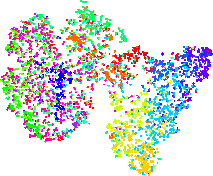
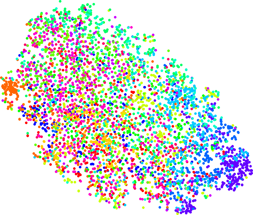
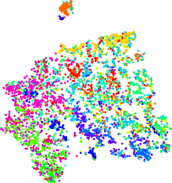
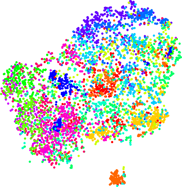
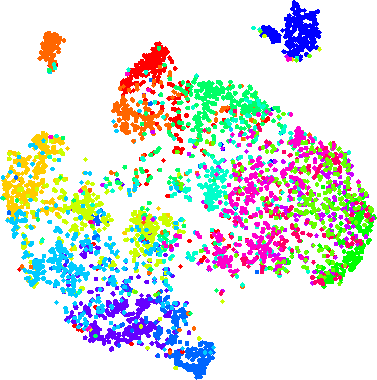
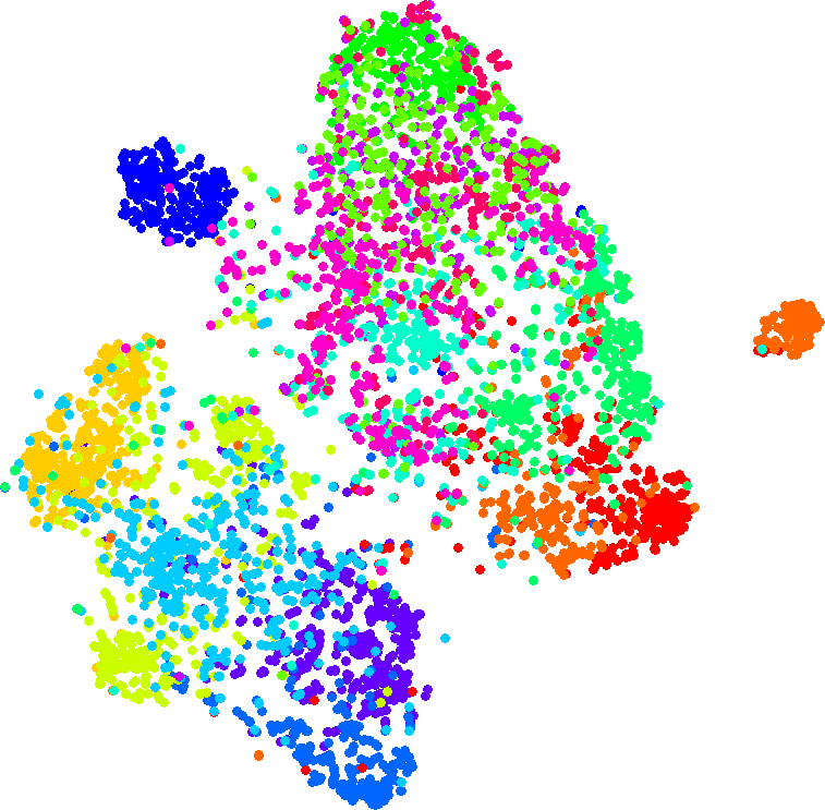
(a) GIST	(b) PHOG	(c) LBP	(d) concatenation	(e) early fusion	(f) late fusion

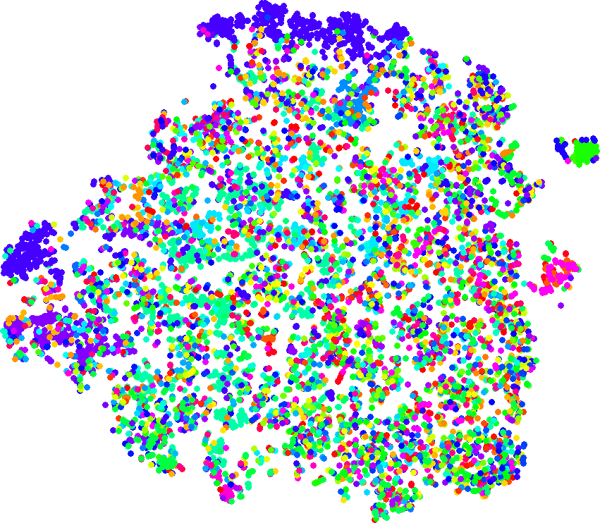
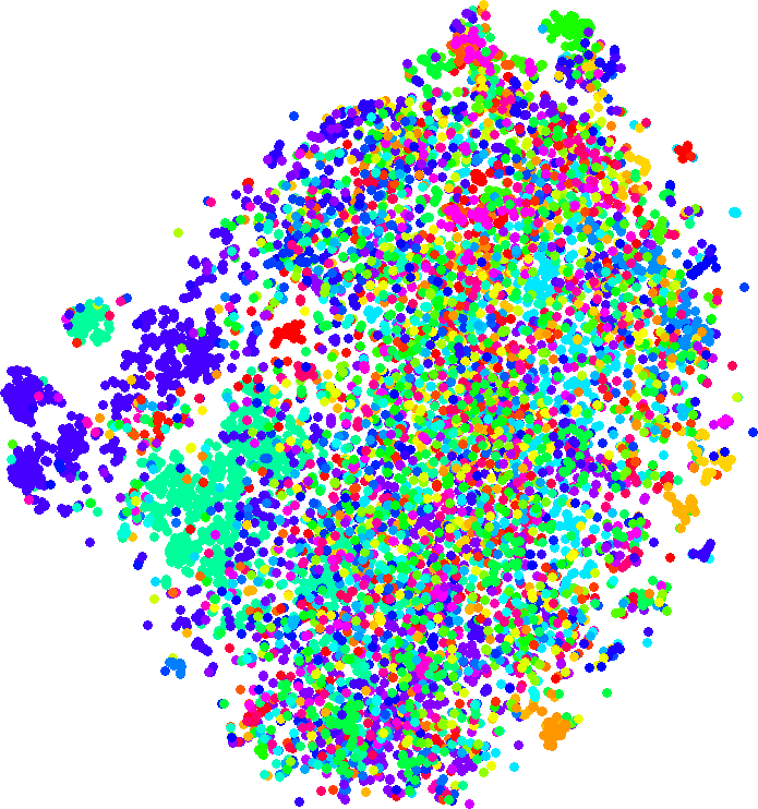
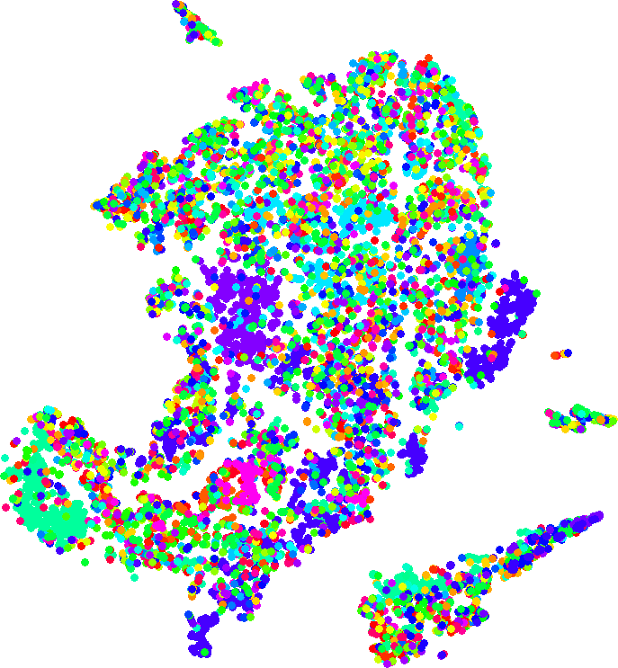
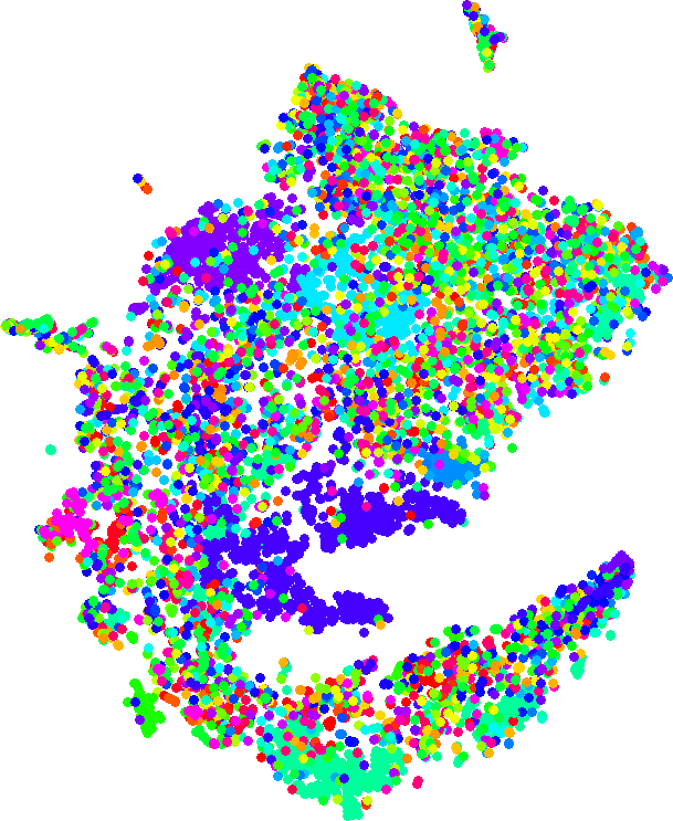
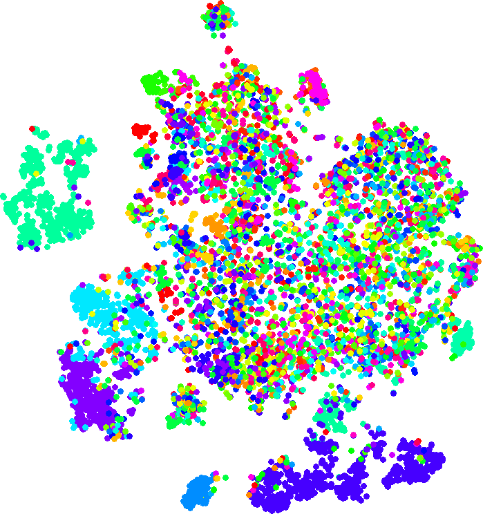
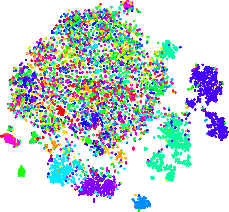
Figure 3: t-SNE 2D projections for the different features used. They are relative to the Scene-15 (top row) and Caltech-101 (bottom row) data sets. Different classes are represented in different colors, and the same class with the same color across the row.

Unsupervised representation learning allows t-SNE to identify groups of images of the same class. Moreover, representations based on early and late fusion induce different relationships among the classes. For instance, in the second row of Fig. 3f the blue and the light green classes have been placed close to each other on the bottom right; in Fig. 3e, instead, the two classes are well separated. The difference in the two representations explains the effectiveness of co-training and justifies the difference in performance between CURL-EF(EP+LR) and CURL-LF(EP+LR).

As further investigation, we also combined the two classifiers produced by the co-training procedure obtaining two other variants of CURL that we denoted as CURL-EF&LF(EP+LR) and CURL-EF&LF_n(EP+LR). However, in our experiments, these variants did not caused any significant improvement when compared to CURL-LF(EP+LR).

V-A Performance across co-training rounds

Here we analyze in more details the performance of our strategy across the five co-training rounds. Results are reported in Fig. 4 with lines of increasing color saturation corresponding to rounds one to five. CURL-LF(EP+LR) is reported in red lines, while CURL-LF_n(EP+LR) in blue.

Scene-15 inductive	Scene-15 transductive	Scene-15 self-taught
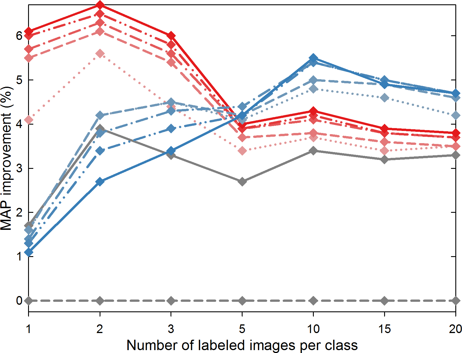
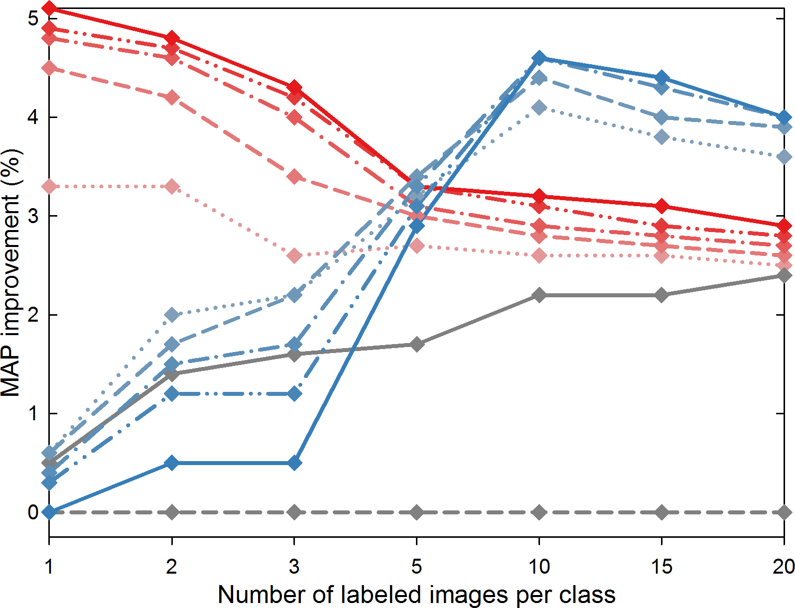
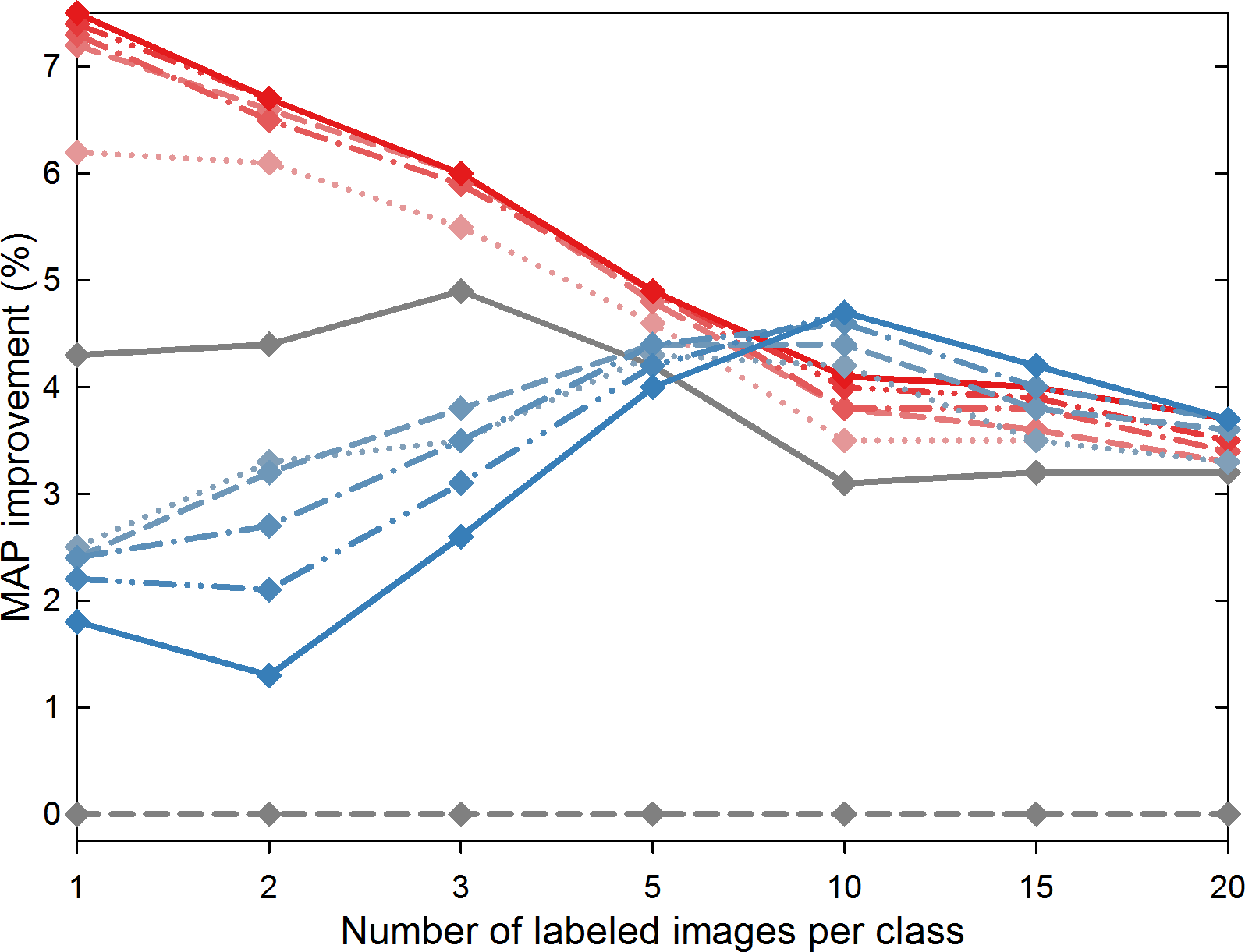
Caltech-101 inductive	Caltech-101 transductive	Caltech-101 self-taught

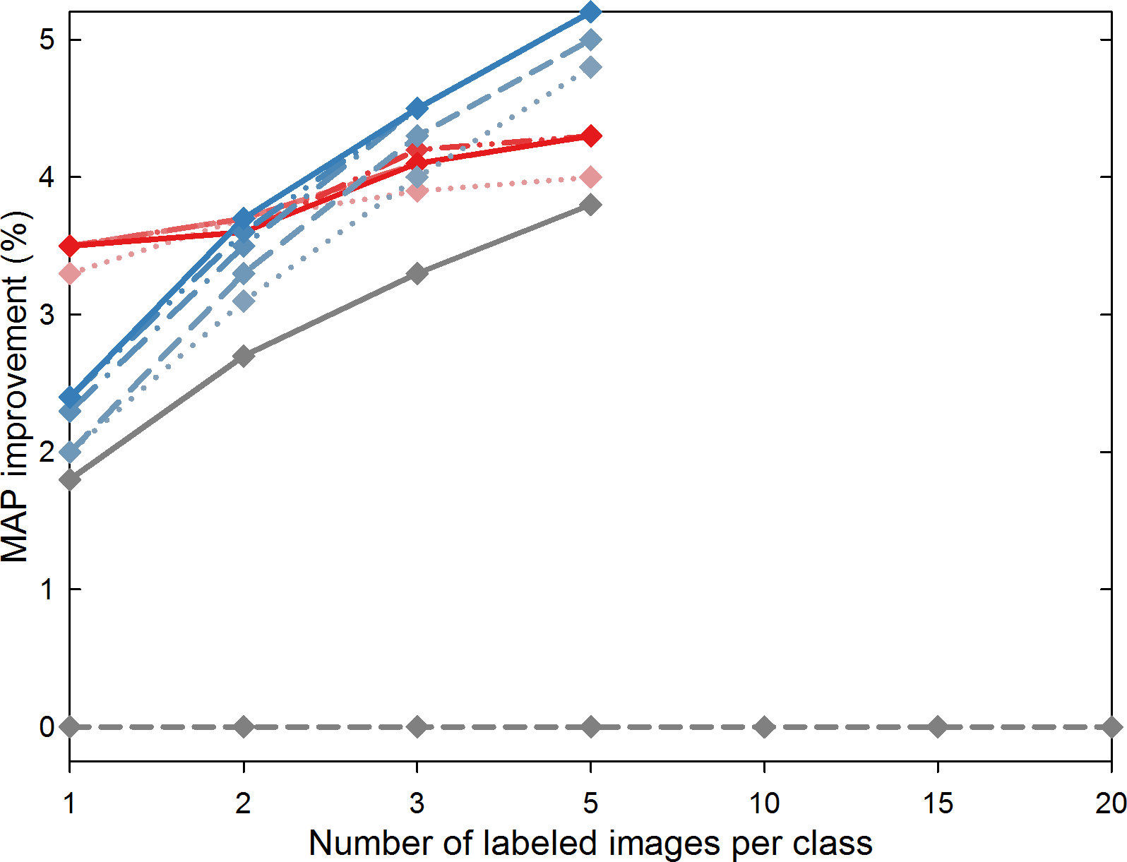
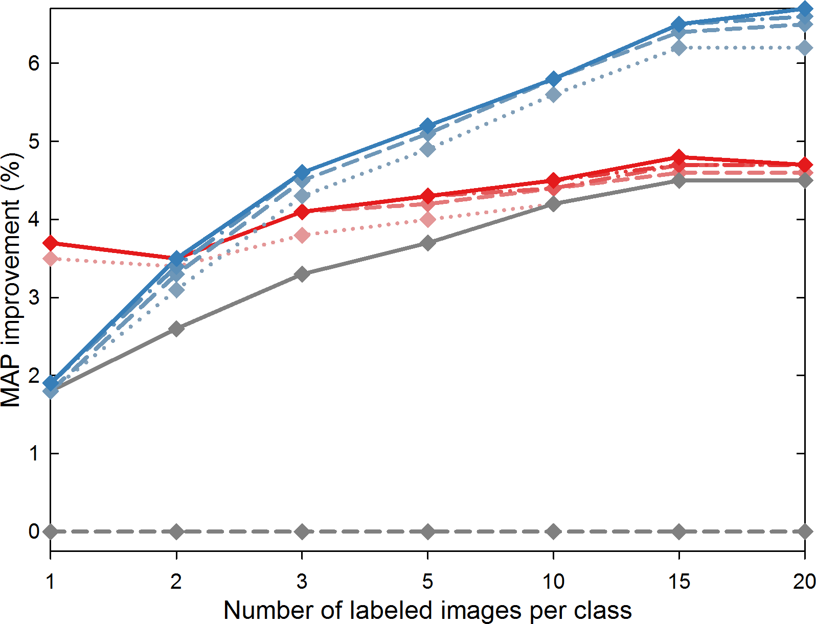
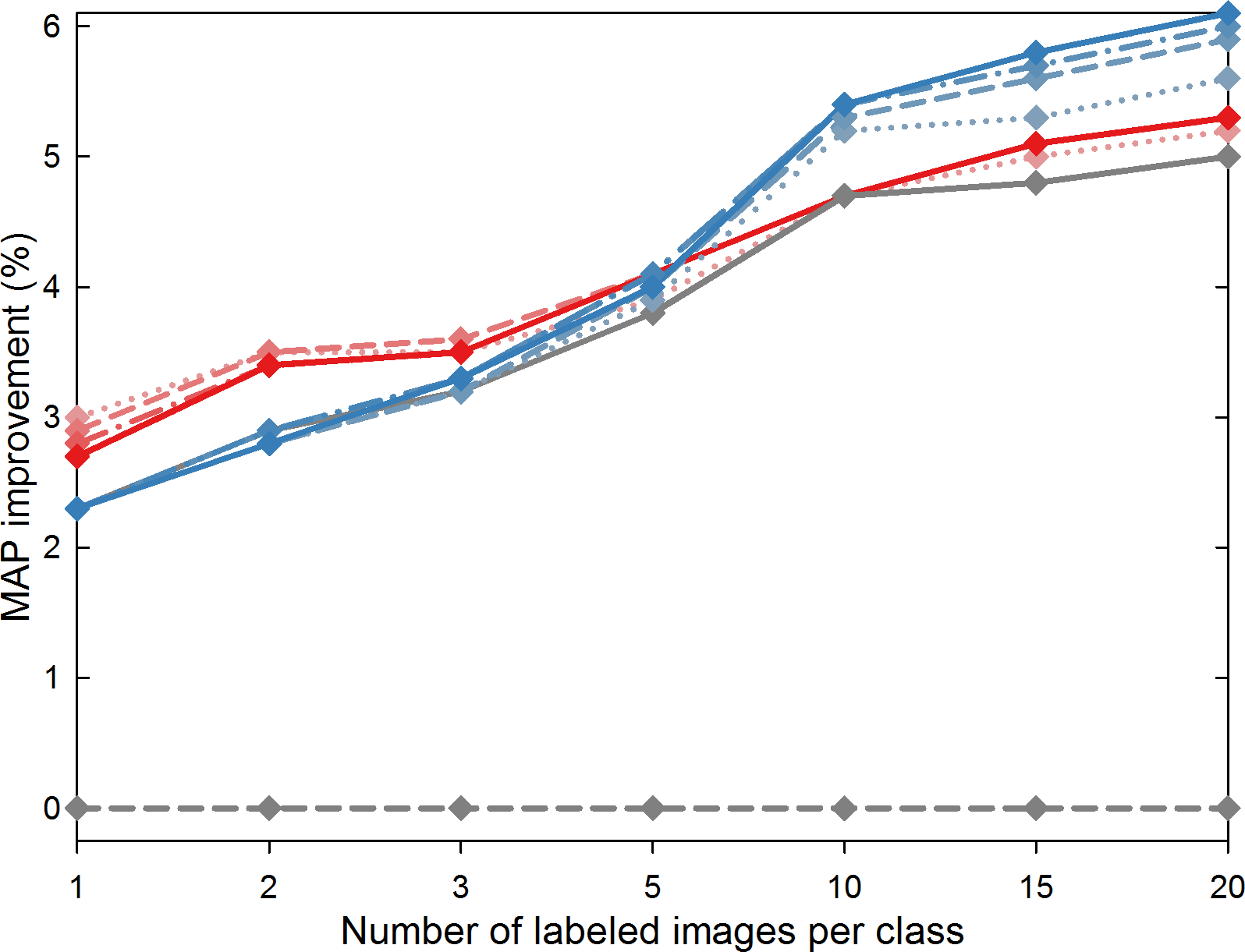
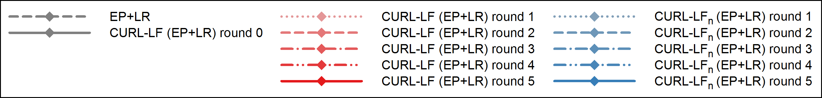
Figure 4: Performance obtained by CURL-LF(EP+LR) and CURL-LF_n(EP+LR) varying the number of co-training rounds. Performance are reported in terms of MAP improvement with respect to Ensemble Projection. Due to the small cardinality of some classes, inductive learning on the Caltech-101 has been limited to five labeled images per class.

Results are reported in terms of MAP improvements with respect to EP+LR, which, we recall, corresponds to CURL-EF(EP+LR) with zero co-training rounds. For CURL-LF(EP+LR), performances always increase with the number of rounds. For CURL-LF_n(EP+LR), this is not true on the Scene-15 data set with a small number of labeled examples. In CURL-LF_n(EP+LR) each round of co-training adds all the promising unlabeled samples, with a high chance of including some of them with the wrong pseudo-label. This may result in a ‘concept drift’, with the classifiers being pulled away from the concepts represented by the labeled examples. This risk is lower on the Caltech-101 (which tends to have more homogeneous classes than Scene-15) and when there are more labeled images. The original CURL-LF(EP+LR) is more conservative, since each of its co-training rounds adds a single image per class. As a result, increasing the rounds usually increases MAP and never decreases it by an appreciable amount.

We observed the same behavior for CURL-EF(EP+LR) and CURL-EF_n(EP+LR). We omit the relative figures for sake of brevity.

The plots confirm that CURL-LF(EP+LR) is better suited for small sets of labeled images, while CURL-LF_n(EP+LR) is to be preferred when more labeled examples are available. The representation learned from late fused features explains part of the effectiveness of CURL. In fact, even CURL-LF(EP+LR) without co-training (zero rounds) outperforms the baseline represented by Ensemble Projection.

V-B Leveraging CNN features in CURL

In this further experiment we want to test if the proposed classification strategy works when more powerful features are used. Recent results indicate that the generic descriptors extracted from pre-trained Convolutional Neural Networks (CNN) are able to obtain consistently superior results compared to the highly tuned state of the art systems in all the visual classification tasks on various datasets [57]. We extract a 4096-dimensional feature vector from each image using the Caffe [60] implementation of the deep CNN described by Krizhevsky et al. [61]. The CNN was discriminatively trained on a large dataset (ILSVRC 2012) with image-level annotations to classify images into 1000 different classes. Briefly, a mean-subtracted $227\times 227$ RGB image is forward propagated through five convolutional layers and two fully connected layers. Features are obtained by extracting activation values of the last hidden layer. More details about the network architecture can be found in [61, 60].

We leverage the CNN features in CURL using them as a fourth feature in addition to the three used in Section IV. The discriminative power of these CNN features alone can be seen in Fig. 5, where their 2D projections obtained applying the t-SNE [59] method are reported.

Scene-15	Caltech-101

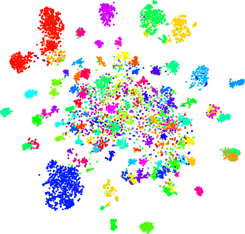
Figure 5: 2D projections for the CNN features on the two data sets used: Scene-15 (left) and Caltech-101 (right). Different classes are represented in different colors.

The experimental results using the four features, are reported in Fig. 6, for both the Scene-15 and Caltech-101 data sets. We report the results in the transductive scenario only. It can be seen that the results using the four features are significantly better than those using only three features mainly due to the discriminative power of the CNN features. Furthermore, the CURL variants achieve better results than the baselines. This suggests that CURL is able to effectively leverage both low/mid level features as LBP, PHOG and GIST, and more powerful features as CNN.

Scene-15 transductive	Caltech-101 transductive

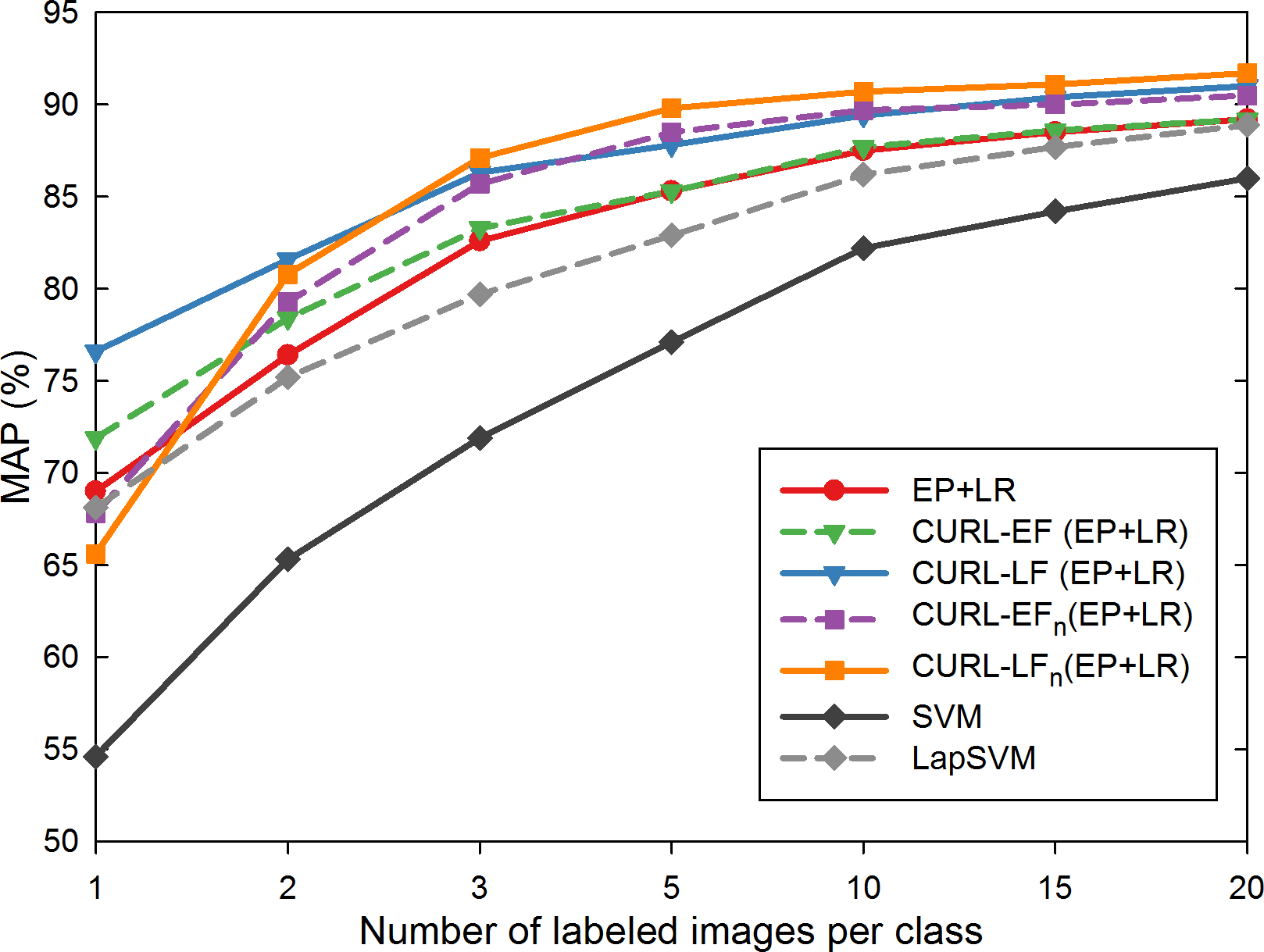
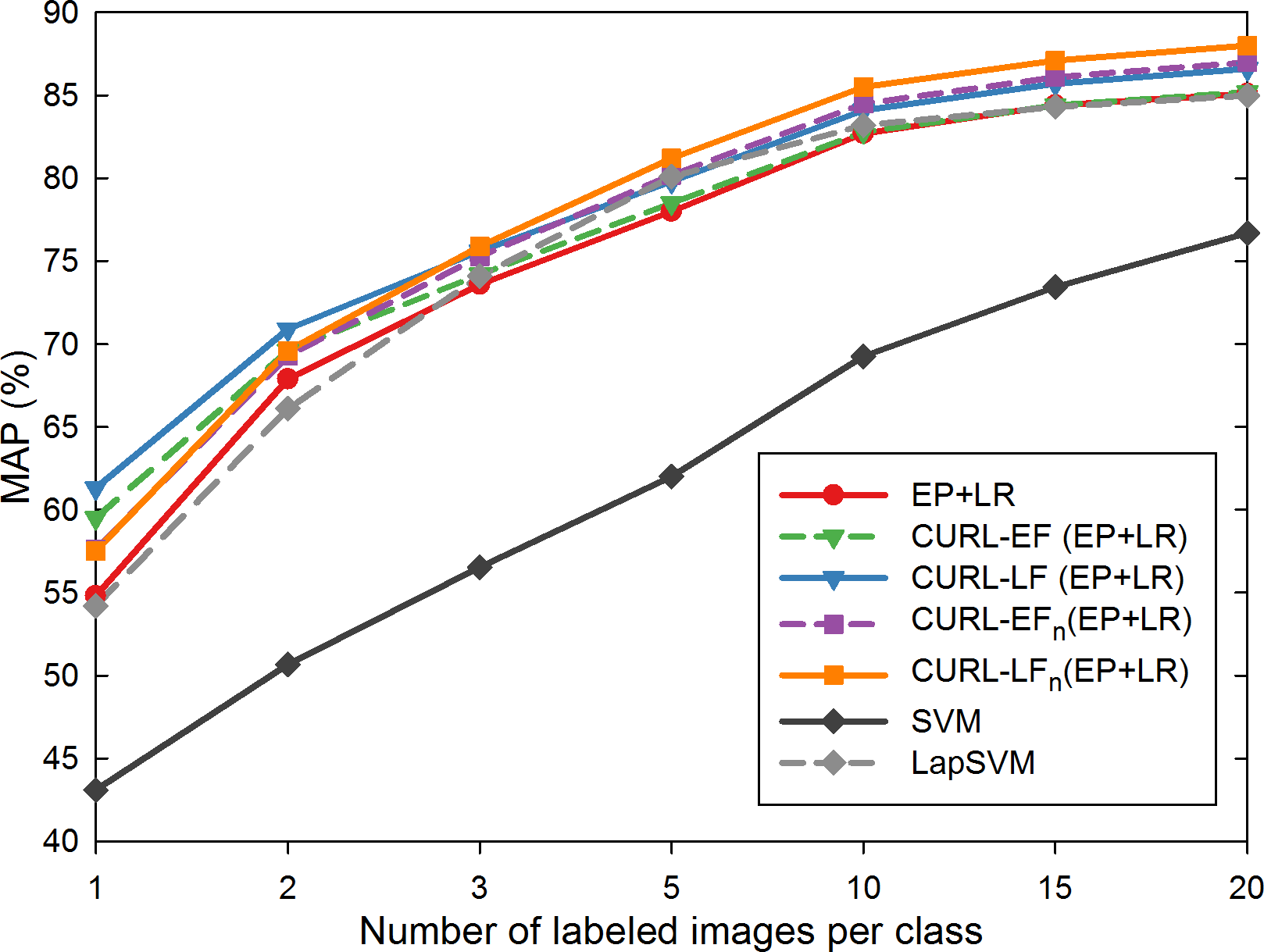
Figure 6: Mean Average Precision (MAP) varying the number of labeled images per class, obtained on the Scene-15 data set (left), and on the Caltech-101 data set (right). Results are obtained using GIST, PHOG, LBP and CNN features.

V-C Second embodiment of CURL using LapSVM

In this Section we want to evaluate the CURL performance in a different embodiment. Specifically, we substitute the EP and LR components with LapSVM-based ones. In the LapSVM, first, an unsupervised geometrical deformation of the feature kernel is performed. This deformed kernel is then used for classification by a standard SVM thus by-passing an explicit definition of a new feature representation. In this CURL embodiment we exploit the unsupervised step as surrogate of the URL component, and SVM as C component. The EF view is obtained concatenating the GIST, PHOG, LBP and CNN features and generating the corresponding kernel, while the LF one is obtained by a linear combination of the four kernels computed on each feature. This is similar to what is done in multiple kernel learning [49]. Due to its performance in the previous experiments, the $\chi^{2}$ kernel is used for both views. The experimental results on the Scene-15 and Caltech-101 data sets in the transductive scenario, are reported in Fig. 7. We named the variants of this CURL embodiment by adding the suffix (LapSVM). It can be seen that the behavior of the different methods is the same of the previous plots, with the LapSVM-based CURL outperforming the standard LapSVM. The plots confirm that CURL-LF(LapSVM) is better suited for small sets of labeled images, while CURL-LF_n(LapSVM) is to be preferred when more labeled examples are available.

Scene-15 transductive	Caltech-101 transductive

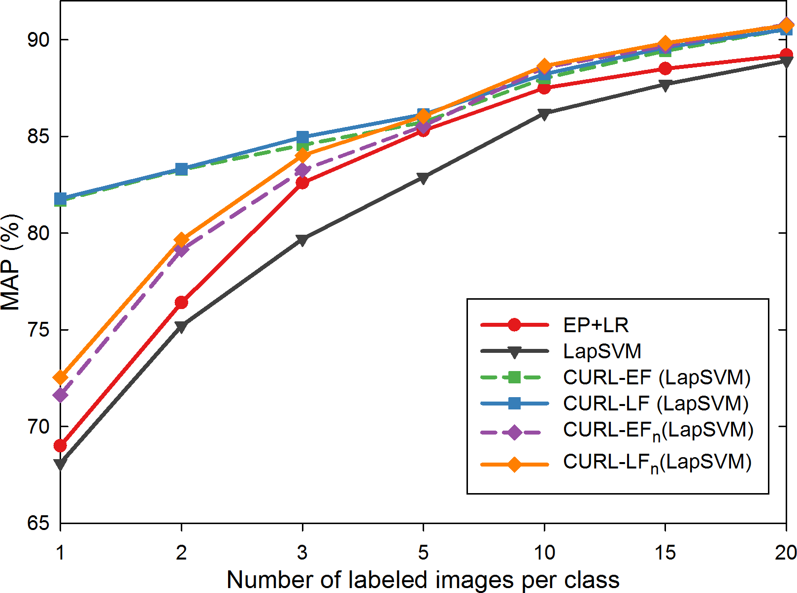
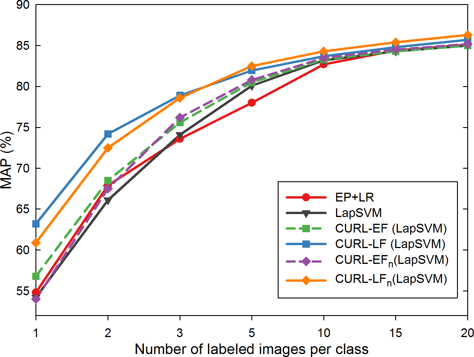
Figure 7: Mean Average Precision (MAP) varying the number of labeled images per class, obtained on the Scene-15 data set (left), and on the Caltech-101 data set (right). Results are obtained using GIST, PHOG, LBP and CNN features.

In Fig. 9 and 10 qualitative results for the ‘Panda’ class of the Caltech-101 data set are reported: the results are relative to the case in which a single instance is available for training and one single example is added at each co-training round (i.e. each pair of rows correspond to CURL-EF(LapSVM) and CURL-LF(LapSVM) respectively). The left part of Fig. 9 contains the training examples that are added by the CURL-EF(LapSVM) and CURL-LF(LapSVM) at each co-training round, while the right part and Fig. 10 contain the first 40 test images ordered by decreasing classification confidence. Samples belonging to the current class are surrounded by a green bounding box, while a red one is used for samples belonging to other classes.

In the sets of training images, it is possible to see that after the first co-training round, CURL-LF(LapSVM) selects new examples to add to the training set, while CURL-EF(LapSVM) adds examples seleted by CURL-LF(LapSVM) in the previous round. This is a pattern that we found to occur also in other categories when very small training sets are used.

In the sets of test images, it is possible to see that more and more positive images are recovered. Moreover, we can see how the images belonging to the correct class tends to be classified with increasing confidence and move to the left, while the confidences of images belonging to other classes decrease and are pushed to the right.

V-D Large scale experiment

In this experiment we want to test the proposed classification strategy on a large scale data set, namely the ILSVRC 2012 which contains a total of 1000 different classes. The experiment is run on the ILSVRC 2012 validation set since the training set was used to learn the CNN features. The ILSVRC 2012 validation set, which contains a total of 50 images for each class, has been randomly divided into a training and a test set containing each 25 images per class. Again, different numbers of training images per class were tested (i.e. 1, 2, 3, 5, 10, and 20). The second embodiment of CURL is used in this experiment.

The experimental results are reported in Fig. 8 and represent the average performance over ten runs with random labeled-unlabeled feature splits.

Given the large range of MAP values, the plot of MAP improvements with respect to LapSVM baseline is also reported. It can be seen that the behavior is similar to that of the previous plots, with the LapSVM-based CURL variants outperforming the LapSVM. As for the previous data sets, the plots show that CURL-EF(LapSVM) and CURL-LF(LapSVM) are better suited for small sets of labeled images, while CURL-EF_n(LapSVM)and CURL-LF_n(LapSVM) are to be preferred when more labeled examples are available. It is remarkable that the proposed classification strategy is able to improve the results of the LapSVM, since the CNN features were specifically learned for the ILSVRC 2012.

ILSVRC 2012 transductive	ILSVRC 2012 transductive

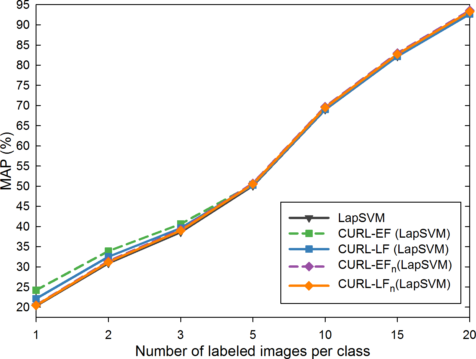
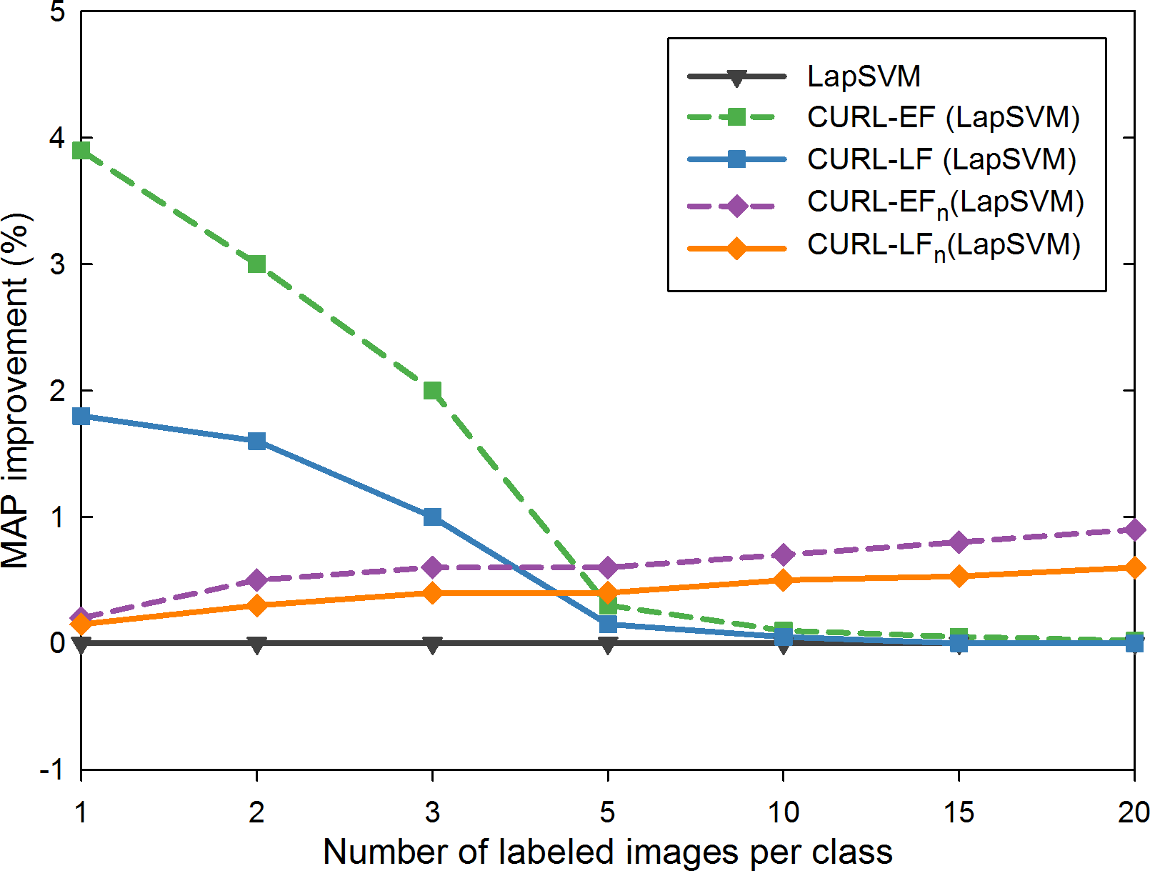
Figure 8: Mean Average Precision (MAP) varying the number of labeled images per class, obtained on the ILSVRC 2012 data set: MAP values (left) and MAP improvements over LapSVM baseline (right). Results are obtained using GIST, PHOG, LBP and CNN features.

\begin{overpic}[height=296.30743pt]{qualitativePanda_40_2s_A.jpg}\put(0.0,47.0){\rotatebox{90.0}{\scriptsize round 0}} \put(1.5,51.0){\scriptsize EF} \put(1.5,47.0){\scriptsize LF} \put(0.0,38.0){\rotatebox{90.0}{\scriptsize round 1}} \put(1.5,42.0){\scriptsize EF} \put(1.5,38.0){\scriptsize LF} \put(0.0,29.0){\rotatebox{90.0}{\scriptsize round 2}} \put(1.5,33.0){\scriptsize EF} \put(1.5,29.0){\scriptsize LF} \put(0.0,20.0){\rotatebox{90.0}{\scriptsize round 3}} \put(1.5,24.0){\scriptsize EF} \put(1.5,20.0){\scriptsize LF} \put(0.0,11.0){\rotatebox{90.0}{\scriptsize round 4}} \put(1.5,15.0){\scriptsize EF} \put(1.5,11.0){\scriptsize LF} \put(0.0,2.0){\rotatebox{90.0}{\scriptsize round 5}} \put(1.5,6.0){\scriptsize EF} \put(1.5,2.0){\scriptsize LF} \put(4.0,55.0){\scriptsize Training images} \put(30.0,55.0){\scriptsize Test images} \end{overpic}

Figure 9: Qualitative results of the proposed strategy for the ‘Panda’ class of the Caltech-101 data set over five co-training rounds. Train images are on the left, the first 17 test images, ordered by decreasing classification confidence are on the right. Test images from 18 to 40 are reported in Fig. 10.

\begin{overpic}[height=296.30743pt]{qualitativePanda_40_2s_B.jpg}\put(1.0,58.0){\scriptsize Test images} \end{overpic}

Figure 10: Qualitative results of the proposed strategy for the ‘Panda’ class of the Caltech-101 data set over five co-training rounds. The images are ordered by decreasing classification confidence. Training image, and test images from 1 to 17 are reported in Fig. 9.

VI Conclusions

In this work we have proposed CURL, a semi-supervised image classification strategy which exploits unlabeled data in two different ways: first two image representations are obtained by unsupervised learning; then co-training is used to enlarge the labeled training set of the corresponding classifiers. The two image representations are built using two different fusion schemes: early fusion and late fusion.

The proposed strategy has been tested on the Scene-15, Caltech-101, and ILSVRC 2012 data sets, and compared with other supervised and semi-supervised methods in three different experimental scenarios: inductive learning, transductive learning, and self-taught learning. We tested two embodiments of CURL and several variants differing in the co-trained classifier used and in the number of pseudo-labeled examples that are added at each co-training round. The experimental results showed that the CURL embodiments outperformed the other methods in the state of the art included in the comparisons. In particular, the variants that add a single pseudo-labeled example per class at each co-training round, resulted to perform best in the case of a small number of labeled images, while the variants adding more examples at each round obtained the best results when more labeled data are available.

Moreover, the results of CURL using a combination of low/mid and high level features (i.e. LBP, PHOG, GIST, and CNN features) outperform those obtained on the same features by state of the art methods. This means that CURL is able to effectively leverage less discriminative features (i.e. LBP, PHOG, GIST) to boost the performance of more discriminative ones (i.e. CNN features).

References

- [1] O. Chapelle, B. Schölkopf, A. Zien et al., Semi-supervised learning. MIT press, 2006.
- [2] K. Nigam, A. McCallum, S. Thrun, and T. Mitchell, “Text classification from labeled and unlabeled documents using em,” Machine learning, vol. 39, no. 2-3, pp. 103–134, 2000.
- [3] A. Fujino, N. Ueda, and K. Saito, “A hybrid generative/discriminative approach to semi-supervised classifier design,” in Proc. of the National Conf. on Artificial Intelligence, 2005, pp. 764–769.
- [4] A. Blum and S. Chawla, “Learning from labeled and unlabeled data using graph mincuts,” in Proc. 18th Int’l Conf. on Machine Learning, 2001, pp. 19–26.
- [5] O. Chapelle, J. Weston, and B. Schölkopf, “Cluster kernels for semi-supervised learning,” in Advances in neural information processing systems, 2002, pp. 585–592.
- [6] T. Joachims, “Transductive inference for text classification using support vector machines,” in Proc. 16th Int’l Conf. on Machine Learning, vol. 99, 1999, pp. 200–209.
- [7] M. Belkin, P. Niyogi, and V. Sindhwani, “Manifold regularization: A geometric framework for learning from labeled and unlabeled examples,” The Journal of Machine Learning Research, vol. 7, pp. 2399–2434, 2006.
- [8] A. Blum and T. Mitchell, “Combining labeled and unlabeled data with co-training,” in Proc. of the 11th annual Conf. on Computational learning theory, 1998, pp. 92–100.
- [9] Z.-H. Zhou and M. Li, “Semi-supervised learning by disagreement,” Knowledge and Information Systems, vol. 24, no. 3, pp. 415–439, 2010.
- [10] G. Iyengar and H. J. Nock, “Discriminative model fusion for semantic concept detection and annotation in video,” in Proceedings of the eleventh ACM international conference on Multimedia, 2003, pp. 255–258.
- [11] P. Gehler and S. Nowozin, “On feature combination for multiclass object classification,” in Computer Vision, 2009 IEEE 12th International Conference on, 2009, pp. 221–228.
- [12] P. Natarajan, S. Wu, S. Vitaladevuni, X. Zhuang, S. Tsakalidis, U. Park, and R. Prasad, “Multimodal feature fusion for robust event detection in web videos,” in Computer Vision and Pattern Recognition (CVPR), 2012 IEEE Conference on, 2012, pp. 1298–1305.
- [13] Z.-H. Zhou and M. Li, “Tri-training: Exploiting unlabeled data using three classifiers,” Knowledge and Data Engineering, IEEE Transactions on, vol. 17, no. 11, pp. 1529–1541, 2005.
- [14] M. Li and Z.-H. Zhou, “Improve computer-aided diagnosis with machine learning techniques using undiagnosed samples,” Systems, Man and Cybernetics, Part A: Systems and Humans, IEEE Transactions on, vol. 37, no. 6, pp. 1088–1098, 2007.
- [15] Z.-H. Zhou, “When semi-supervised learning meets ensemble learning,” Frontiers of Electrical and Electronic Engineering in China, vol. 6, no. 1, pp. 6–16, 2011.
- [16] M. Wang, X.-S. Hua, and Y. Dai, L-R.and Song, “Enhanced semi-supervised learning for automatic video annotation,” in IEEE Int’l Conf. on Multimedia and Expo, 2006, pp. 1485–1488.
- [17] S. Gupta, J. Kim, K. Grauman, and R. Mooney, “Watch, listen & learn: Co-training on captioned images and videos,” in Machine Learning and Knowledge Discovery in Databases, 2008, pp. 457–472.
- [18] A. Levin, P. Viola, and Y. Freund, “Unsupervised improvement of visual detectors using cotraining,” in Proc. of IEEE Int’l Conf. on Computer Vision, 2003, pp. 626–633.
- [19] C. Christoudias, K. Saenko, L. Morency, and T. Darrell, “Co-adaptation of audio-visual speech and gesture classifiers,” in Proc. of the Int’l Conf. on Multimodal interfaces, 2006, pp. 84–91.
- [20] H. Feng and T.-S. Chua, “A bootstrapping approach to annotating large image collection,” in Proc. of the ACM SIGMM Int’l Workshop on Multimedia Information Retrieval, 2003, pp. 55–62.
- [21] H. Bhatt, S. Bharadwaj, R. Singh, M. Vatsa, A. Noore, and A. Ross, “On co-training online biometric classifiers,” in Int’l Joint Conf. on Biometrics, 2011, pp. 1–7.
- [22] S. Tong and E. Chang, “Support vector machine active learning for image retrieval,” in Proc. of ACM Int’l Conf. on Multimedia, 2001, pp. 107–118.
- [23] M. Guillaumin, J. Verbeek, and C. Schmid, “Multimodal semi-supervised learning for image classification,” in IEEE Conf. on Computer Vision and Pattern Recognition, 2010, pp. 902–909.
- [24] O. Javed, S. Ali, and M. Shah, “Online detection and classification of moving objects using progressively improving detectors,” in Computer Vision and Pattern Recognition, 2005. CVPR 2005. IEEE Computer Society Conference on, vol. 1. IEEE, 2005, pp. 696–701.
- [25] F. Tang, S. Brennan, Q. Zhao, and H. Tao, “Co-tracking using semi-supervised support vector machines,” in Computer Vision, 2007. ICCV 2007. IEEE 11th International Conference on. IEEE, 2007, pp. 1–8.
- [26] W. Wang and Z. Zhou, “Analyzing co-training style algorithms,” in Proc. of the European Conf. on Machine Learning, 2007, pp. 454–465.
- [27] S. Goldman and Y. Zhou, “Enhancing supervised learning with unlabeled data,” in Proc. of the Int’l Conf on Machine Learning, 2000, pp. 327–334.
- [28] M. Chen, Y. Chen, and K. Q. Weinberger, “Automatic feature decomposition for single view co-training,” in Proceedings of the 28th International Conference on Machine Learning (ICML-11), 2011, pp. 953–960.
- [29] W. Wang and Z.-H. Zhou, “Co-training with insufficient views,” in Asian Conference on Machine Learning, 2013, pp. 467–482.
- [30] W. Wang and Z. Zhou, “A new analysis of co-training,” in Proc. of the Int’l Conf on Machine Learning, 2010, pp. 1135–1142.
- [31] G. Hinton, S. Osindero, and Y. Teh, “A fast learning algorithm for deep belief nets,” Neural computation, vol. 18, no. 7, pp. 1527–1554, 2006.
- [32] K. Jarrett, K. Kavukcuoglu, M. Ranzato, and Y. LeCun, “What is the best multi-stage architecture for object recognition?” in IEEE Int’l Conf. on Computer Vision, 2009, pp. 2146–2153.
- [33] G. Hinton, “Training products of experts by minimizing contrastive divergence,” Neural computation, vol. 14, no. 8, pp. 1771–1800, 2002.
- [34] H. Bourlard and Y. Kamp, “Auto-association by multilayer perceptrons and singular value decomposition,” Biological cybernetics, vol. 59, no. 4-5, pp. 291–294, 1988.
- [35] Y. Bengio, “Learning deep architectures for ai,” Foundations and trends in Machine Learning, vol. 2, no. 1, pp. 1–127, 2009.
- [36] A. Coates and A. Y. Ng, “Learning feature representations with k-means,” in Neural Networks: Tricks of the Trade, 2012, pp. 561–580.
- [37] G. Csurka, C. Dance, L. Fan, J. Willamowski, and C. Bray, “Visual categorization with bags of keypoints,” in ECCV Workshop on statistical learning in computer vision, 2004, pp. 1–2.
- [38] S. Lazebnik, C. Schmid, and J. Ponce, “Beyond bags of features: Spatial pyramid matching for recognizing natural scene categories,” in IEEE Conf. on Computer Vision and Pattern Recognition, vol. 2, 2006, pp. 2169–2178.
- [39] B. A. Olshausen and D. Field, “Sparse coding with an overcomplete basis set: A strategy employed by v1?” Vision research, vol. 37, no. 23, pp. 3311–3325, 1997.
- [40] J. Mairal, F. Bach, J. Ponce, and G. Sapiro, “Online learning for matrix factorization and sparse coding,” The J. of Machine Learning Research, vol. 11, pp. 19–60, 2010.
- [41] M. Lewicki and T. Sejnowski, “Learning overcomplete representations,” Neural computation, vol. 12, no. 2, pp. 337–365, 2000.
- [42] D. Dai and L. V. Gool, “Ensemble projection for semi-supervised image classification,” in Computer Vision (ICCV), 2013 IEEE International Conference on. IEEE, 2013, pp. 2072–2079.
- [43] P. K. Atrey, M. A. Hossain, A. El Saddik, and M. S. Kankanhalli, “Multimodal fusion for multimedia analysis: a survey,” Multimedia systems, vol. 16, no. 6, pp. 345–379, 2010.
- [44] C. G. Snoek, M. Worring, and A. W. Smeulders, “Early versus late fusion in semantic video analysis,” in Proceedings of the 13th annual ACM international conference on Multimedia. ACM, 2005, pp. 399–402.
- [45] W. S. Noble et al., “Support vector machine applications in computational biology,” Kernel methods in computational biology, pp. 71–92, 2004.
- [46] S. Ayache, G. Quénot, and J. Gensel, Classifier fusion for SVM-based multimedia semantic indexing. Springer, 2007.
- [47] Z. Wu, L. Cai, and H. Meng, “Multi-level fusion of audio and visual features for speaker identification,” in Advances in Biometrics. Springer, 2005, pp. 493–499.
- [48] G. R. Lanckriet, N. Cristianini, P. Bartlett, L. E. Ghaoui, and M. I. Jordan, “Learning the kernel matrix with semidefinite programming,” The Journal of Machine Learning Research, vol. 5, pp. 27–72, 2004.
- [49] M. Gönen and E. Alpaydın, “Multiple kernel learning algorithms,” The Journal of Machine Learning Research, vol. 12, pp. 2211–2268, 2011.
- [50] D.-H. Lee, “Pseudo-label: The simple and efficient semi-supervised learning method for deep neural networks,” in Workshop on Challenges in Representation Learning, ICML, 2013.
- [51] M.-F. Balcan, A. Blum, and K. Yang, “Co-training and expansion: Towards bridging theory and practice,” in Advances in neural information processing systems, 2004, pp. 89–96.
- [52] L. Fei-Fei, R. Fergus, and P. Perona, “Learning generative visual models from few training examples: An incremental bayesian approach tested on 101 object categories,” Computer Vision and Image Understanding, vol. 106, no. 1, pp. 59–70, 2007.
- [53] J. Deng, W. Dong, R. Socher, L.-J. Li, K. Li, and L. Fei-Fei, “Imagenet: A large-scale hierarchical image database,” in Computer Vision and Pattern Recognition, 2009. CVPR 2009. IEEE Conference on. IEEE, 2009, pp. 248–255.
- [54] A. Oliva and A. Torralba, “Modeling the shape of the scene: A holistic representation of the spatial envelope,” International journal of computer vision, vol. 42, no. 3, pp. 145–175, 2001.
- [55] A. Bosch, A. Zisserman, and X. Muoz, “Image classification using random forests and ferns,” in Computer Vision, 2007. ICCV 2007. IEEE 11th International Conference on, Oct 2007, pp. 1–8.
- [56] T. Ojala, M. Pietikainen, and T. Maenpaa, “Multiresolution gray-scale and rotation invariant texture classification with local binary patterns,” Pattern Analysis and Machine Intelligence, IEEE Transactions on, vol. 24, no. 7, pp. 971–987, 2002.
- [57] A. S. Razavian, H. Azizpour, J. Sullivan, and S. Carlsson, “Cnn features off-the-shelf: an astounding baseline for recognition,” in Computer Vision and Pattern Recognition Workshops (CVPRW), 2014 IEEE Conference on. IEEE, 2014, pp. 512–519.
- [58] V. Sindhwani, P. Niyogi, and M. Belkin, “Beyond the point cloud: from transductive to semi-supervised learning,” in Proceedings of the 22nd international conference on Machine learning. ACM, 2005, pp. 824–831.
- [59] L. Van der Maaten and G. Hinton, “Visualizing data using t-sne,” Journal of Machine Learning Research, vol. 9, no. 2579-2605, p. 85, 2008.
- [60] Y. Jia, E. Shelhamer, J. Donahue, S. Karayev, J. Long, R. Girshick, S. Guadarrama, and T. Darrell, “Caffe: Convolutional architecture for fast feature embedding,” in Proceedings of the ACM International Conference on Multimedia. ACM, 2014, pp. 675–678.
- [61] A. Krizhevsky, I. Sutskever, and G. E. Hinton, “Imagenet classification with deep convolutional neural networks,” in Advances in neural information processing systems, 2012, pp. 1097–1105.