Turbulence on a Fractal Fourier Set

Abstract

A novel investigation of the nature of intermittency in incompressible, homogeneous and isotropic turbulence is performed by a numerical study of the Navier-Stokes equations constrained on a fractal Fourier set. The robustness of the energy transfer and of the vortex stretching mechanisms is tested by changing the fractal dimension, $D$, from the original three dimensional case to a strongly decimated system with $D=2.5$, where only about $3\%$ of the Fourier modes interact. This is a unique methodology to probe the statistical properties of the turbulent energy cascade, without breaking any of the original symmetries of the equations. While the direct energy cascade persists, deviations from the Kolmogorov scaling are observed in the kinetic energy spectra. A model in terms of a correction with a linear dependency on the codimension of the fractal set, $E(k)\sim k^{-5/3+3-D}$, explains the results. At small scales, the intermittency of the vorticity field is observed to be quasisingular as a function of the fractal mode reduction, leading to an almost Gaussian statistics already at $D\sim 2.98$. These effects must be connected to a genuine modification in the triad-to-triad nonlinear energy transfer mechanism.

Understanding and controlling the energy transfer process in turbulent flows is a key problem for a broad range of fields, such as astrophysics biskamp , atmospheric or ocean sciences pedlosky , mathematics and engineering pope_book . The main obstacle hampering theoretical, numerical, and phenomenological advancements is intermittency: the presence of strong non-Guassian and out-of-equilibrium velocity fluctuations in a wide range of scales frisch ; Kr71 ; Kr74 ; MK00 ; SreFa06 . The energy cascade is fully chaotic, nonlinear and driven by the vortex-stretching mechanism, i.e., the tendency of the flow to amplify vorticity in thin, long filaments. A long debate exists whether or not the presence of such geometrical structures is correlated to the non-Gaussian statistics observed at small scales frisch . Many authors have focused on a vortex-by-vortex analysis, looking for the signatures of quasisingularities or extreme events due to specific dynamical properties of the Navier-Stokes (NS) equations chorin ; pullin ; PPSAM95 ; Tsi97 ; Pi99 ; Luthi05 ; Ka15 . Other approaches are based on a Fourier description, such as closure K61 ; orszag77 and renormalization-group theories DDM ; eyink ; antonov .
In this Letter, we investigate the origin of intermittency in turbulent flows by a novel strategy. The idea consists of modifying the nonlinear interactions of Navier-Stokes equations, without introducing extra forces and without breaking the symmetries of the original equations, such as statistical homogeneity, isotropy and rescaling properties in the inviscid limit. To achieve this, we adopt a recently proposed numerical methodology frisch2012 to solve NS equations on a preselected, multiscale (fractal) set of Fourier modes. This allows us to control the number of degrees of freedom participating in the non-linear dynamics by changing one free parameter only, the fractal dimension of the Fourier set, $D$. For $D=3$, the original problem is recovered. In the sequel, we describe the methodology, the numerical setup and the main results concerning the quasisingular effect of fractal mode reduction on the small-scale intermittency.
Methodology. Fractal mode reduction is realized via the Fourier decimation operator ${\cal P}^{D}$, acting in the space of divergece-free velocity fields as follows frisch2012 . We define ${\bf v}({\bf x},t)$ and ${\bf u}({\bf k},t)$ as the real and Fourier space representation of the velocity field in $D=3$, respectively. The decimated field, ${\bf v}^{D}({\bf x},t)$, is obtained as:

$${\bf v}^{D}({\bf x},t)={\cal P}^{D}{\bf v}({\bf x},t)=\sum_{{\bf k}\in{\cal Z}^{3}}e^{i{\bf k\cdot x}}\,\gamma_{\bf k}{\bf u}({\bf k},t)\,.$$ (1)

The random numbers $\gamma_{{\bf k}}$ are quenched in time and are:

$$\gamma_{\bf k}=\begin{cases}1,&\text{with probability}\ h_{k}\,,\\ 0,&\text{with probability}\ 1-h_{k},k\equiv|{\bf k}|\,.\end{cases}$$ (2)

The choice for the probability $h_{k}\propto(k/k_{0})^{D-3}$, with $0<D\leq 3$ ensures that the dynamics is isotropically decimated to a $D$-dimensional Fourier space. The factors $h_{k}$ are chosen independently and preserve Hermitian symmetry $\gamma_{k}=\gamma_{-k}$ so that ${\cal P}^{D}$ is self-adjoint. The NS equations for the velocity field decimated on a fractal Fourier set are then defined as:

$$\partial_{t}{\bf v}^{D}={\cal P}^{D}N({\bf v}^{D},{\bf v}^{D})+\nu\,\nabla^{2}{\bf v}^{D}+{\bf f}^{D}\,.$$ (3)

At each iteration the nonlinear term, $N({\bf v},{\bf v})=-{\bf v}\cdot{\bf{\nabla v}}-{\bf\nabla}p$, is projected on the quenched fractal set, to constrain the dynamical evolution to evolve on the same Fourier skeleton at all times. Similarly, the initial condition and the external forcing must have a support on the same set of Fourier modes. Let us notice that the projection acts as a self-similar Galerkin truncation. In the $(L^{2})$ norm, $\|{\bf v}\|\propto\int|{\bf v}({\bf x})|^{2}d^{3}x$, the self-adjoint operator ${\cal P}^{D}$ commutes with the gradient and viscous operators. Since ${\cal P}^{D}{\bf v}^{D}={\bf v}^{D}$, it then follows that both energy and helicity are conserved in the inviscid and unforced limit, exactly as in the original problem with $D=3$. As a result of the Fourier decimation, the velocity field is embedded in a three dimensional space, but effectively possesses a number of Fourier modes that grows slower with decreasing $D$. The degrees of freedom inside a sphere of radius $k$ go as $\#_{dof}(k)\sim k^{D}$.
This idea, introduced for the first time in (frisch2012, ), has been used to test the hypothesis that two-dimensional turbulence in the inverse energy cascade approaches a quasiequilibrium state (lvov, ). Fourier decimation methods are not new for hydrodynamics: we mention protocols with a specific degree of mode reduction (GLR96, ; MPPZ96, ; DLE07, ), and the extreme truncation criterion of shell models for the turbulent energy cascade bif03 . Results are puzzling. For NS equations at small Reynolds numbers GLR96 , intermittency strongly depends on the amount of scales resolved in the inertial range. However, in the case of shell models, intermittency is observed to be a function of the effective dimension giuliani , and coinciding with the one measured in the original NS equations paladin-vulpiani , when energy and helicity are the two inviscid invariants. Note that fractal Fourier mode-reduction changes also the relative population of local-to-nonlocal triadic interactions Kr71 , since triads with all modes in the high wave number range have a larger probability to be decimated. Furthermore, being an exquisitely dynamical approach, it is different from a posteriori filtering techniques, largely exploited to analyze turbulent data farge .
A pseudospectral method is adopted to solve Eqs. (3) in a periodic box of length $L=2\pi$ at resolution $N=1024^{3}$ and $2048^{3}$, dealiased with the two-thirds rule; time stepping is implemented with a second-order Adams-Bashforth scheme. A large-scale forcing pope keeps the total kinetic energy constant in a range of shells, $0.7\leq|{\bf k}|<1.7$, leading to a steady, homogeneous and isotropic flow. We performed direct numerical simulation (DNS) runs by changing the fractal dimension $2.5\leq D\leq 3$, the spatial resolution, the viscosity and the realization of the fractal, quenched mask. Table 1 summarizes the relevant parameters.

$D$	$3$	$2.999$	$2.99$	$2.99$	$2.98$	$2.98$	$2.8$	$2.5$
$N$	$1024$	$1024$	$1024$	$2048$	$1024$	$2048$	$1024$	$1024$
$M_{r}$	$100\%$	$99\%$	$93\%$	$92\%$	$87\%$	$85\%$	$25\%$	$3\%$
$\eta$	$0.75$	$0.75$	$0.95$	$0.70$	$0.75$	$0.70$	$0.90$	$0.65$
${\cal N}_{T}$	10	10	11	10	11	7	10	20
$E$	$3.1$	$3.1$	$3.1$	$3.3$	$3.3$	$3.5$	$4.1$	$5.4$
$\nu\cdot 10^{4}$	$6.0$	$6.0$	$6.0$	$2.0$	$6.0$	$2.0$	$6.0$	$1.5$
$Re\cdot 10^{-3}$	$3.9$	$3.9$	$3.8$	$11.8$	$3.9$	$12.1$	$4.0$	$15.4$

Table 1: DNS parameters. $D$: fractal dimension; $N$: grid resolution; $M_{r}$: percentage of surviving Fourier modes; $\eta$: Kolmogorov length scale in unit of the grid spacing $\Delta x=L/N$; ${\cal N}_{T}$: number of large-scale eddy-turnover-times in the steady state; $E$: total kinetic energy $\langle v^{2}\rangle/2$; $\nu$: viscosity; $Re$: Reynolds number $Re=E^{1/2}{\cal L}/\nu$, where the integral scale ${\cal L}$ is estimated from the kinetic energy spectrum.

Results. The starting point of our analysis is the shell-to-shell energy transfer in the Fourier space. Following the notation adopted in Ref. Kr71 , we write the energy spectrum for a generic flow in dimension $D$ as:

$$E^{D}(k)=\int_{|{\bf k}_{1}|=k}d^{3}k_{1}\gamma_{{\bf k}_{1}}\int d^{3}k_{2}\gamma_{{\bf k}_{2}}\langle{\bf u}({\bf k}_{1})\,{\bf u}({\bf k}_{2})\rangle\,,$$ (4)

where the decimation factor $\gamma_{{\bf k}}$ takes into account that the Fourier mode ${\bf k}$ is active with probability $h_{\bf k}$. Similarly, we can write for the energy flux across a Fourier mode $k$, $\Pi^{D}(k)=\int_{|{\bf k}_{1}|<k}d^{3}k_{1}\partial_{t}E(k_{1})$:

$$\Pi^{D}(k)=\int_{|{\bf k}_{1}|<k}d^{3}k_{1}\gamma_{{\bf k}_{1}}\int d^{3}k_{2}d^{3}k_{3}\gamma_{{\bf k}_{2}}\gamma_{{\bf k}_{3}}S({\bf k}_{1}|{\bf k}_{2},{\bf k}_{3}),$$ (5)

where the explicit form of the symmetric triadic correlation function is RoseSulem : $S({\bf k}_{1}|{\bf k}_{2},{\bf k}_{3})=-Im[\langle({\bf k}_{1}\cdot{\bf u}({\bf k}_{3}))({\bf u}({\bf k}_{1})\cdot{\bf u}({\bf k}_{2}))\rangle+\langle({\bf k}_{1}\cdot{\bf u}({\bf k}_{2}))({\bf u}({\bf k}_{1})\cdot{\bf u}({\bf k}_{3}))\rangle]$. Supposing a power-law behavior of the velocity fluctuations $u(k)\sim k^{-a}$, we can predict a self-similar scaling of the energy flux as $\Pi^{D}(\lambda k)\sim\lambda^{3D+1-3a}\Pi^{D}(k)$. In this expression, the rescaling factor $\lambda^{3D}$ is due to the integral over the variables $({\bf k}_{1},{\bf k}_{2},{\bf k}_{3})$, while $\lambda^{1-3a}$ comes from the triadic nonlinear term.
If a constant energy flux develops in the inertial range of scales, the following dimensional relation holds:

$$a=D+1/3\rightarrow E^{D}(k)\sim k^{3-D}\,E^{K41}(k)\,,$$ (6)

where $E^{K41}(k)\sim k^{-5/3}$ is the Kolmogorov 1941 spectrum expected for the original case with $D=3$. In the previous dimensional argument, the tiny intermittent corrections to the spectrum scaling exponent are neglected IsGoKa09 , while prefactors are omitted for simplicity. The relation (6) is obtained by noticing that, because of homogeneity, we have that $\langle\,{\bf u}({\bf k}_{1})\cdot{\bf u}({\bf k}_{2})\,\rangle\propto F({\bf k}_{1})\delta^{3}({\bf k}_{1}+{\bf k}_{2})$, and by also noticing that the decimation projector verifies the identity $(\gamma_{{\bf k}})^{2}=\gamma_{{\bf k}}$.

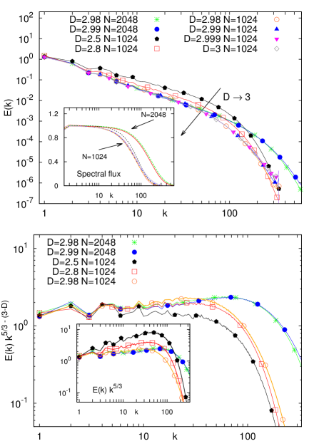
Figure 1: (Top): Log-Log plot of the mean kinetic energy spectra for different $D$; in the inset, the mean kinetic energy fluxes. (Bottom): Compensated energy spectra $E^{D}(k)\,k^{5/3-3+D}$ vs the wave number $k$; in the inset, the compensation is done with the Kolmogorov prediction, $E^{D}(k)\,k^{5/3}$.

As a result, the dynamical effect of Fourier decimation is to make the energy spectrum shallower than the Kolmogorov one for three-dimensional turbulence, also predicting the existence of a critical dimension $D=7/3$, when the spectrum becomes ultraviolet divergent frisch in the limit of zero viscosity. By decreasing $D$ in the presence of a forward energy cascade, the system has fewer modes available to transfer the same amount of energy (see Table 1), and the velocity field becomes increasingly rougher.
In the upper panel of Fig. 1, we plot the energy spectra and the associated energy fluxes, for all DNS. It shows that when increasing the grid resolution for fixed $D$, from $N=1024$ to $N=2048$, no appreciable differences are observed, indicating that the presence of a forward energy cascade appears robust and Reynolds independent. In the lower panel we also show that the spectra compensate well with the prediction (6), while they fail to satisfactorily compensate with the classical K41 prediction when $D<3$. We stress that the latter result is significant for $D=2.5$ and $D=2.8$ only. For the other dimensions $D$, the effect is so small that it might fall within the intermittent correction of the original Navier-Stokes case at $D=3$. Moreover, the effect of the quenched disorder is robust: spectra obtained with different realizations of the mask do not show any statistically significant difference (not shown).
Figure 1 (upper inset) shows that, when decreasing the fractal dimension $D$, the mean energy transfer towards small scales is almost unchanged, i.e. the hypothesis leading to the relation (6) is well verified. On the other hand, temporal fluctuations of the energy flux increase with $D$ (not shown).
It might be argued that the effect of fractal Fourier decimation is purely geometrical and that the main dynamical processes are unchanged. To show that this is not the case, it is useful to analyze the effect of a static Fourier decimation.

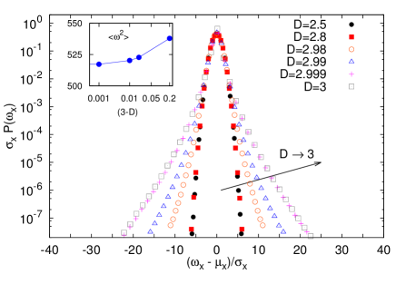
Figure 2: Probability density function of the vorticity component $\omega_{x}$, normalized to its standard deviation. Data refer to simulations at resolution $N=1024$. In the inset, mean square vorticity $\langle w^{2}\rangle$ versus the fractal dimension deficit, $3-D$.

This can be done by considering snapshots of $D=3$ turbulence, and applying the fractal decimation as an a posteriori filter. It is immediate to realize that the effect of the static decimation on the spectrum is $E^{D}_{st}(k)\sim k^{D-3}\,E^{K41}(k)$, implying that the geometrical action of the decimation goes in the opposite direction of the dynamical one.
We now consider the dynamical effect of the fractal Fourier decimation on the small-scale structures, by focusing on the statistics of the vorticity field in the real space. In Fig. 2 we plot the probability density function (PDF) of the vorticity field, normalized with its standard deviation. We note that already at $D=2.99$, vorticity fluctuations have changed their intensity of 1 order of magnitude, despite the fact that the mean enstrophy is practically unchanged. Even more remarkable, intermittent fluctuations disappear already at $D=2.8$, where a quasi-Gaussian vorticity PDF is measured. The transition towards Gaussianity is better quantified considering the vorticity kurtosis. In Fig. 3, we compare results of the fractally decimated NS equations, with those obtained from the application of the a posteriori static mask on three-dimensional turbulence. The dynamical decimation makes a very fast transition towards a Gaussian behaviour, such that at $D=2.98$ the kurtosis has decreased by 30$\%$, to already approach the Gaussian value at $D=2.8$. In the case of thea posteriori static decimation, vorticity kurtosis assumes the Gaussian value only at $D=2.5$, while staying almost unchanged in the range $D\geq 2.98$. Such a strong difference clearly indicates that constraining the dynamics to a subset of modes is critical for the complete development of intermittency in real space.
In Fig. 4, we plot the kurtosis of the longitudinal velocity increment, $K(\delta v_{r})=\langle(\delta_{r}{\bf v}\cdot\hat{\bf r})^{4}\rangle/\langle(\delta_{r}{\bf v}\cdot\hat{\bf r})^{2}\rangle^{2}$. Notice the sharp transition leading to an almost scale-independent, nonintermittent behavior for $D<3$. Moreover, at fixed fractal dimension, the effects of increasing the Reynolds number is to further reduce the intermittent corrections.
Conclusions. Fractal mode-reduction is a new route to design numerical simulations to tackle the problem of intermittency and to potentially develop multiscale models of turbulence. The first non trivial result is the robustness of the energy flux under modereduction. An inertial range of scales with a constant-flux solution is observed when $D$ is changed and few Fourier modes survive, at least in the parameter range investigated here. This is in agreement with the observation that Galerkin truncations do not alter the inviscid conservation of quadratic quantities, preserving the existence of exact scaling solutions for suitable third-order correlation functions (see appendix of Ref. biferale_jfm ). The Fourier spectrum gets a power law correction that can be predicted by a dimensional argument.

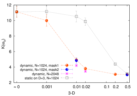
Figure 3: Lin-log plot of vorticity kurtosis vs the dimension deficit $3-D$. The upper curve is obtained from the application of the a posteriori static mask on $D=3$ velocity field snapshots. The lower curve comes from the Fourier decimated DNS. Data for $D=2.99$ and $D=2.5$, with a different realization of the fractal projection, are indistinguishable. Data at resolution $N=2048$ are also plotted.

Second and more striking, small-scale intermittency is quickly reduced for $D<3$ and it almost vanishes already at $D=2.98$. As a consequence, the presence or absence of some of the Fourier modes strongly modify the fluctuations of all the others, suggesting the possibility that intermittency is the result of percolating dynamical properties across the whole Fourier lattice bustamante .
Because of the spectrum modification, the scaling exponent of the second order longitudinal structure function becomes $\zeta_{2}+(D-3)$, where $\zeta_{2}$ is the measured in the $D=3$ homogeneous and isotropic case. This observation would suggest that, for the dimension deficit $3-D<1$, one may obtain corrections to the scaling exponents proportional to $3-D$, and the anomalous exponents might be computed perturbatively in the dimension deficit. If this is the case, the critical dimension $D_{c}$ is estimated as the value of $D$ where the dimensional scaling is recovered, namely $\zeta_{2}+D_{c}-3=2/3$. It gives $D_{c}\sim 2.96$ not far from the value of $D$ at which intermittency is observed to vanish in the DNS. However, there is no reason to assume that anomalous exponents can be computed perturbatively in $3-D$. In fact, as mentioned above, intermittency might well be the result of multiscale interactions in Fourier space, needing all degrees of freedom to develop. Hence, in the presence of even a tiny decimation, NS singular solutions responsible for the anomalous scaling no longer exist. This would also explain why we observe, Fig. 4, a reduction of intermittency by increasing the resolution at fixed $D$.

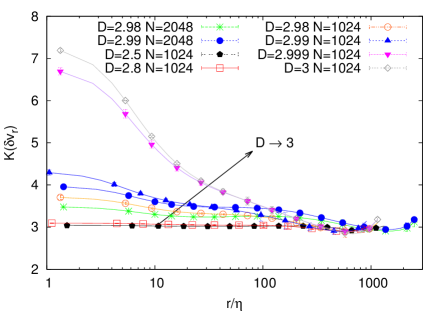
Figure 4: Lin-log plot of longitudinal velocity increment kurtosis $K(\delta v_{r})$ vs the scale separation normalised by the Kolmogorov scale, $r/\eta$. For all data sets, error bars are within the symbol width.

Additionally, phenomenological cascade models frisch would be unable to explain the results, as well.
In the light of our results, Fourier decimation can also be seen as a way to introduce a control parameter and modify the scaling properties of the system, similarly to what happens for NS equations stirred by a random, power-law forcing FNS77 ; FF78 ; prlnoi ; noiNJP04 ; pandit . In the latter case, perturbative or semianalytic calculations mou ; muratore give indications on the reasons why anomalous corrections should cancel out for specific values of the control pararameter. Also, in Ref.prlnoi it is numerically shown that when the random injection becomes the dominant scaling contribution in the inertial range, a transition to a Gaussian statistics is observed for the velocity increments. In the present case, however, the connections between the observed transition to a Gaussian behavior, and a possible renormalised perturbation theory are to be explored.

We acknowledge useful discussions with S. Musacchio and P. Perlekar, who collaborated with us in the first part of the work. DNS were done at CINECA (Italy), within the EU-PRACE Project Pra04, No.806. This work is part of the activity of the ERC AdG NewTURB, No.339032. We thank F. Bonaccorso and G. Amati for technical support. We thank the COST-Action MP1305 for support.

References

- (1) D. Biskamp, Magnetohydrodynamic Turbulence (Cambridge University Press, Cambridge, England 2008).
- (2) J. Pedlosky, Geophysical Fluid Dynamics, (Springer-Verlag, New York, 1987).
- (3) S. B. Pope, Turbulent Flows, (Cambridge University Press, Cambridge, England, 2000).
- (4) U. Frisch, Turbulence (Cambridge University Press, Cambridge, England, 1995).
- (5) R. H. Kraichnan, J. Fluid Mech. 47, 525 (1971).
- (6) R. H. Kraichnan, J. Fluid Mech. 62, 305 (1974).
- (7) C. Meneveau and J. Katz, Annu. Rev. Fluid Mech. 32, 1–32 (2000).
- (8) G. Falkovich and K.R. Sreenivasan, Phys. Today 59 No. 4, 43 (2006).
- (9) A.J. Chorin, Comm. Math. Phys. 83 517 (1982).
- (10) D. I. Pullin and P.G. Saffman, Annu. Rev. Fluid Mech. 30 51 (1998).
- (11) T. Passot, H. Politano, P.-L. Sulem, J. R. Angilella and M. Meneguzzi, J. Fluid Mech. 282, 313 (1995).
- (12) A. Tsinober, L. Shtilman and H. Vaisburd, Fluid Dyn. Res. 21, 477 (1997).
- (13) P. Chainais, P. Abry and J.-F. Pinton, Phys. Fluids 11, No 11, 3524 (1999).
- (14) B. Lüthi, A. Tsinober, and W. Kinzelbach, J. Fluid Mech. 528, 87 (2005).
- (15) K. Yoshimatsu, K. Anayama, and Y Kaneda, Phys. Fluids 27, 055106 (2015).
- (16) R. H. Kraichnan, J. Math. Phys. 2, 124 (1961).
- (17) S. A. Orszag, in Lectures on the Statistical Theory of Turbulence, in Fluid Dynamics, Proceedings of the Les Houches Summer School 1973, edited by R. Balian and J. L. Peube, (Gordon and Breach, New York).
- (18) C. De Dominicis and P. C. Martin, Phys. Rev. A 19, 419 (1979).
- (19) G. L. Eyink, Phys. Fluids 6, 3063 (1994).
- (20) L.Ts Adzhemyan, N.V. Antonov, A.N. Vasiliev, “The Field Theoretic Renormalization Group in Fully Developed Turbulence”, (Gordon and Breach, New York, 1989).
- (21) U. Frisch, A. Pomyalov, I. Procaccia, and S. S. Ray, Phys. Rev. Lett. 108, 074501 (2012).
- (22) V. S. Lvov, A. Pomyalov, and I. Procaccia, Phys. Rev. Lett. 89, 064501 (2002).
- (23) S. Grossmann, D. Lohse, and A. Reeh, Phys. Rev. Lett. 77,5369 (1996).
- (24) M. Meneguzzi, H. Politano, A. Pouquet, and M. Zolver, J. Comput. Phys. 132, 32 (1996).
- (25) F. De Lillo and B. Eckhardt, Phys. Rev. E 76, 016301 (2007).
- (26) L. Biferale, Annu. Rev. Fluid. Mech. 35, 441 (2003).
- (27) P. Giuliani, M.H. Jensen, and V. Yakhot, Phys. Rev. E 65, 036305 (2002).
- (28) M.H. Jensen, G. Paladin, A. Vulpiani, Phys. Rev. A 43, 798 (1991).
- (29) M. Farge, Annu. Rev. Fluid Mech. 24, (1992).
- (30) A. G. Lamorgese, D. A. Caughey, and S. B. Pope, Phys. Fluids 17, 015106 (2005).
- (31) H. A. Rose and P. L. Sulem, J. Phys. France 39, 441 (1978).
- (32) T. Ishihara, T. Gotoh and Y. Kaneda, Annu. Rev. Fluid Mech. 41, 165 (2009).
- (33) J. Harris, C. Connaughton and M.D. Bustamante, New J. Phys. 15, 083011 (2013).
- (34) L.Biferale, S. Musacchio, and F. Toschi, J. Fluid Mech. 730, 309 (2013).
- (35) D. Forster, D. R. Nelson, and M. J. Stephen, Phys. Rev. A 16, 732 (1977).
- (36) J. D. Fournier and U. Frisch, Phys. Rev. A 17, 747 (1978).
- (37) L. Biferale, A. S. Lanotte, and F. Toschi, Phys. Rev. Lett. 92, 094503 (2004).
- (38) L. Biferale, M. Cencini, A. S. Lanotte, M. Sbragaglia, and F. Toschi, New J. Phys. 6, 37 (2004).
- (39) A. Sain, Manu and R. Pandit, Phys. Rev. Lett. 81, 4377 (1998).
- (40) C.-Y. Mou and P. B. Weichman, Phys Rev. E 52, 3738 (1995).
- (41) C. Mejia-Monasterio, and P. Muratore-Ginanneschi, Phys. Rev. E 86, 016315 (2012).