†Department of Statistics, School of Mathematics, Statistics and computer Science,
College of Science, University of Tehran, P.O. Box 14155-6455, Tehran, Iran
‡Department of Statistics, Allameh Tabataba’i University, Tehran, Iran
Abstract
We introduce the problem of estimation of the parameters of a dynamically selected population in an infinite
sequence of random variables and provide its application in the statistical inference based
on record values from a non-stationary scheme.
We develop unbiased estimation of the parameters of the dynamically selected population
and evaluate the risk of the estimators. We provide comparisons with natural estimators and
obtain asymptotic results. Finally, we illustrate the applicability of the results using real data.
Keywords: Extreme value theory,
General record models, Partial maxima, Pfeifer model, Selected population, Uniformly minimum
variance unbiased estimator.
1 Introduction
The problem of estimating parameters of selected populations has wide practical
applications in estimation of experimental data in agriculture, industry and medicine.
Some of the real world applications of this theory are the
problem of estimating the average yield of a selected variety of plant with maximum yield (Kumar and Kar, 2001), estimating the average fuel efficiency of the
vehicle with minimum fuel consumption (Kumar and Gangopadhyay, 2005) and selecting the regimen with maximal efficacy or minimal toxicity from a
set of regimens and estimating a treatment effect for the selected regimen (Sill and Sampson, 2007).
The problem of estimation
after selection has received considerable attention by many
researches in the past three decades. Interested readers are referred to, for example, Gibbons et
al. (1977) for more details. Some other
contributions in this area include Sarkadi (1967), Dahiya (1974), Kumar
and Kar (2001), Misra et al. (2006a,b), Kumar et al. (2009) and Nematollahi and Motammed-Shariati (2012). For
a summary of results, as well as a list of references until 2006, see Misra et
al. (2006 a,b).
In this paper, we introduce and develop the problem of estimation
of the parameters of a dynamically selected population
from a sequence of infinite populations which
is not studied in the literature, according to the best of our knowledge.
Let be a sequence of random variables where
is drawn from population with corresponding cumulative
distribution function (cdf) and probability
density function (pdf) . The traffic volume trend, daily temperatures,
sequences of stock quotes, or sequences of
estimators of interior water volume in a dam reservoir are examples
of such sequences.
Suppose we want to estimate the parameter of the population
corresponding to the largest value of the sequence
yet seen, that is
where , with probability one, and for
or similarly the parameter of the population corresponding to the
smallest value of the sequence yet seen, that is
where , with probability one, and for
We want to estimate , and similarly the lower ones .
This happens for example, when we want to estimate the largest value of traffic volume
or stock quotes yet seen, the
temperature of the coldest day or the largest volume of the
coming water into the dam reservoir, up to now.
For simplicity, we denote by hereafter.
We may write
(1)
where
(4)
(5)
The statistics and are called upper and lower records, respectively.
In the sequence , the sequences of partial
maxima and upper record statistics are defined by and , respectively, where with
probability 1, and for
. The record statistics could be
viewed as the dynamic maxima of the original random variables. So, we call the
problem of estimating as the estimation of the parameter of a dynamically selected population.
There is a vast literature on records for iid as well as non-stationary random variables.
A thorough survey of available results,
until 1998, is given in the book of Arnold et al. (1998).
More recent articles on record values include, among others,
Amini and Balakrishnan (2013, 2015), Doostparast and Emadi (2013), Salehi et al. (2013),
Ahmadi and Balakrishnan (2013, 2010), Psarrakos and Navarro (2013),
Raqab and Ahmadi (2012), Zarezadeh and Asadi (2010), Kundu et al. (2009) and Baklizi (2008).
This problem is related to the so-called general record
model. The geometrically increasing
populations, the Pfeifer, the linear drift and the record models are some of the generally used record models.
The basics of non-stationary schemes for the record values are
due to Nevzorov (1985, 1986) and Pfeifer (1989, 1991),
who considered the so-called -scheme, that is the
sequences of independent random variables with distribution
, where is a
continuous cdf and ’s are positive parameters. Further
generalization of the -scheme was suggested by Ballerini and
Resnick (1987). Although non-stationary schemes could be employed in
the most general setting, the special case of improving populations is usually of special interest. Alternative
non-stationary schemes include geometrically increasing populations,
linear trend and Pfeifer models.
In all the above
models, strict assumptions are made on the sequence of parameters
. For instance, in record
model, the sequence of the parameters is assumed to be known or depend
on a fixed unknown parameter. In the linear drift model, a linearly
increasing population is assumed as the underlying population.
However, certain natural phenomena may behave otherwise. For example, an
earthquake is produced by a natural phenomenon which has a pivotal parameter that
varies based on an unknown model. In order to
predict extremely destructive earthquakes, a very important question
is on the value of the parameters which cause a
new record in the sequence of earthquakes?
This motivates us to study the problem of dynamic after-selection
estimation.
The rest of this paper is organized as follows. The theoretical results of the dynamic after-selection
problem, consisting unbiased estimation of the parameters of the
model as well as unbiased estimation of the risk of the estimators
are presented in Sections 2 and 3. In Section 4,
we compare the proposed estimators with some natural estimators.
Asymptotic distributional results for studying the limiting behavior
of the risks of the estimators
are studied in Section 5. Finally, a real
data example is considered in section 6 to illustrate the
applicability of the results.
2 Minimum variance unbiased estimation
Let , and be a random parameter (a function of and ). Suppose that
is estimated by . Following Lehmann (1951), the estimator is said to be risk unbiased for under the loss function , if it satisfies
In this section, we use the U-V method of Robbins (1988), to find Uniformly Minimum Variance Unbiased (UMVU) estimator of
under the two models 1 and 2, presented below.
Model 1: Let be a sequence of
independent absolutely continuous random variables with pdf
(8)
where is a complete sufficient statistic with the
Gamma)-distribution. Some well-known members of the
above family are:
1. Exponential(), with , and
;
2. Gamma(), with and ;
3. Normal(0,), with
, , and
;
4. Inverse Gaussian(), with , , and
;
5. Weibull(), with known , , , and
;
6. Rayleigh(), with , , and
.
To estimate in the family of distributions (8), we first consider the estimation of
under the Gamma()-distribution with pdf
(9)
By using the U-V
method of Robbins (1988), we have the following lemma (see also
Vellaisamy and Sharma, 1989).
Lemma 1
Let be a sequence of independent random variables
with densities defined in (9). Let
be a real-valued function such that for
(i)
(ii)
Then the functions
satisfy
The next result obtains the unbiased estimator of
, under the SEL function, for the Gamma() distribution with the pdf of as in (9).
Theorem 1
For the Gamma() distribution with the pdf of as in (9),
an unbiased estimator of
, under SEL function, which satisfies (7) with , is
(10)
where is the upper record value of the sequence .
Proof
From (1), (4) and Lemma 1, an unbiased
estimator of , under SEL function, based on
is given by
To find an unbiased estimator of under the Model 1 with the pdf of as in (8), let , and . Then, by replacing with in Theorem 1, an unbiased
estimator of , under the SEL function, for the general family (8), can be obtained as
(11)
where is the upper record value of the sequence .
For a monotone function (available in all of the above
examples, except in the normal distribution), can be obtained simply as for an increasing
and as for a decreasing . For example, for the
Rayleigh()-distribution, an unbiased estimator for
is
Model 2: For , consider
two families of distributions, the first with having the survival function
(12)
and the second with having the cdf
(13)
in which is a cdf, free of , and
. We assume to be known. These are called proportional hazard rate and proportional reversed hazard rate families, or simply models
in the context of record values. Some
well-known members of the above families are:
By making use of U-V method of Robbins (1988) for the family
(12), we have the following lemma.
Lemma 2
Let be a sequence of independent random variables
with survival function defined in (12). Let
be a real-valued function such that for
(i)
(ii)
in which is the hazard function of and is the
corresponding pdf of . Then the functions
satisfy
Proof
For one component problem (i.e., a single random variable , ), let . Then, we have
For the sequence , the result follows by a similar calculation.
The next result gives the unbiased estimator of
, under SEL function, for the general family (12).
Theorem 2
Assume to be known and let be the cumulative hazard function of . For the general family (12), an unbiased estimator of
, under the SEL function, is
(14)
Proof
From (1), (4) and Lemma 2, an unbiased estimator
of is given by
Remark 1
Similarly, for the family (13),
an unbiased estimator for , under the SEL function, is
where is the cumulative reversed hazard function of the known cdf .
Remark 2
Note that is a complete sufficient statistic
for . Hence, the above
unbiased estimators of are indeed UMVU estimators of
.
3 Estimation of the Risks
To compare the UMVU estimator with other estimators, we need to compute
the risk function of the proposed estimators.
Under the SEL function, the risk of an estimator is
The UMVU estimators obtained in Section 3 are functions of
. Suppose
we want to estimate the risk of an estimator of which
depend on only through and , i.e.
. Then, we have the following results, under
Models 1 and 2, respectively.
Theorem 3
Under the Model 1 and the SEL function, an unbiased estimator of the risk of an
estimator of is
Proof
From Lemma 1 with , we have
where
Therefore
Furthermore
Which completes the proof.
An immediate corollary of Theorem 3
is as follows.
Corollary 1
Under the Model 1 and the SEL function, an unbiased estimator of the risk of
is
Theorem 4
For the general family (12), and under the SEL function, an unbiased
estimator of the risk of an estimator of
is
Proof
From Lemma 2 and using similar argument as in the proof of Theorem 3, we have
Furthermore
This completes the proof.
An immediate
corollary of Theorem 4 is as follows.
Corollary 2
For the general family (12) and under the SEL function,
(i) an unbiased
estimator of the risk of
is
(ii) the risk of is
Remark 3
The results for the general family (13) can be obtained by
replacing with in Theorem
4 and Corollary 2.
Remark 4
Since is a complete sufficient statistic
for , the above
unbiased estimators of are indeed, UMVU
estimators of .
The following result presents the distribution
of the unbiased estimator in the family (12).
Lemma 3
In the general family (12), the following identities hold:
(i) For every and ,
(ii) For every , and ,
Proof Let and , . We only prove part (i). Part (ii) is proved in a simillar way.
Using the fact that and the lack of memory property of the exponential distribution,
Thus, a natural estimator for , for this family of
distributions is . For the general family with the survival
function (12), we have
which candidates as a natural estimator of .
So a risk comparison of the natural estimators with UMVUEs of
, for both families of distributions is considered.
The following Corollary of Theorem 4 states that, under Model 2, the UMVUE dominates the natural estimator.
Corollary 3
For the general family (12) and under the SEL function, we have
Proof
First, we have
Consequently,
This completes the proof.
However, under Model 1, no explicit results can be obtained for domination of the UMVUE or the natural estimator with respect to the other, since
we have similarly
To compare the UMVUE and the natural estimator under Model 1, we run a simulation study, which is described in the following section.
4.1 Simulation study
We assume . To compare the risks of the UMVUE
, with that of the natural estimator
, for
, , we consider three different models for the sequence of
parameters as follows:
Model 1 (An stochastic, positive error auto-regressive model):
Model 2 (An stochastic Geometrically increasing population):
Model 3 (White noise model):
The simulated bias and risks of the estimators are tabulated in Table 1. As one can observe
from Table 1, the simulated risks of are less than those of .
Also, biases and risks are increasing in , except the risks of , under the white noise
Model 3.
Table 1: Simulated bias and risk of the UMVUE and the natural estimator of under three different models from
gamma distribution for different values of and .
Model 1
2
3
4
0.5
Risk
9.440638
14.75326
18.54895
Bias
1.524951
4.747217
9.160673
Risk
23.1851
84.08421
209.7748
2
Risk
3.224838
6.856674
10.66222
Bias
0.5978639
1.782032
3.29696
Risk
3.886525
12.33907
27.96078
Model 2
2
3
4
0.5
Risk
2.224561
53.26235
1785.95
Bias
0.7864656
2.342428
6.334353
Risk
5.501025
94.40079
2499.64
2
Risk
0.5376576
2.314486
19.68881
Bias
0.3038626
0.72345
1.335166
Risk
0.6209572
2.658157
19.79643
Model 3
2
3
4
0.5
Risk
161.3311
146.8202
125.2359
Bias
13.682
30.34559
47.98977
Risk
685.7074
1851.813
3543.839
2
Risk
64.93679
74.52687
82.06017
Bias
7.023687
13.47608
19.60645
Risk
131.9781
297.2568
537.5641
5 Asymptotic results
From Corollary 2, the risk of the UMVUE of for the general family (12), , is
where is the upper record value form the sequence , with .
Hence, asymptotic joint distribution of and would be useful for computing the risks of the estimators. The following theorem
proposes the required asymptotic distribution.
Theorem 5
Let and be such that
as for all real , where is one of the three extreme value cdfs (see Resnick, 1987, p. 38). Then, for the family (12) with , and letting and , we have, for all ,
as , where is the corresponding pdf of .
Proof. Letting , and
is the order statistic of .
Using the independence of and under the model (Ballerini and Resnick, 1987), we have
Consequently, since satisfies the Von-Mises conditions (see Resnick, 1987) and , as , we have
Thus, the proof is complete.
When is standard exponential distribution, we have , and .
Therefore, letting and , as , we have
and consequently for each and , as , we have
However, and depend on the unknown . The following result solves this problem
using the fact that under the model, converges in law to the standard
normal distribution (see Nevzerov, 1995).
Theorem 6
Under the family (12) with , with the assumptions of Theorem
5, and letting , as , for fixed
, and , we have
where is the cdf of the standard normal distribution.
as , which is the upper Fréchet Höeffding bound; see, e.g., Fréchet (1951) or Nelsen (1999, p. 9).
The following Corollary, presents an approximate formula for the risk of UMVUE of , for the family (12).
Corollary 4
For the family (12), under the assumptions of Theorem 5, we have
The above double integral can be simplified by algebraic manipulations as
in which is the pdf of the standard normal distribution.
Thus, we have
as .
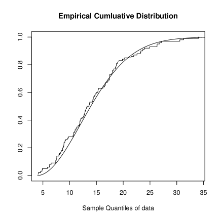
6 Rainfall data: an illustrative example
In this section, we utilize the data set which represents the
records of the amount of annual (January 1-December 31) rainfall in
inches recorded at Los Angeles Civic Center LACC during the 100-year
period from 1890 until 1989, presented by Arnold et al. [1998, p.
180].
A member of the model (Model 2) with survival function as in (12), that is the Rayleigh distribution with cdf
(16)
is well-fitted to the data.
The -value for two-sample Kolmogorov-Smirnov test is 0.3333. Figure 1 shows the empirical distribution function of the rainfall data and the cdf in (16). Thus, we take
to be the known cumulative hazard rate function of the base distribution .
Figure 1: Empirical cdf of the rainfall data.
Suppose that the only observations are the sequence of upper record values as follows:
12.69
12.84
18.72
21.96
23.92
27.16
31.28
34.04.
We consider two hypotheses:
(Stationary model) ;
(Non-stationary model) and s are independent.
Under , , with
probability 1. Hence, is the
UMVUE of . Also, ,
with unbiased estimator .
Under , and the
unbiased estimator of its risk is .
Figure 2 shows the values of and their
corresponding 3- region
under and .
Figure 2: Estimates path (solid line) and 3- regions (upper and lower dashed lines) of , under the stationary (straight lines) and non-stationary (zigzag lines) assumptions, for the rainfall data.
To test against using the record sequence we propose the scale invariant test statistic
(17)
Since, under , all s are equal, the null hypothesis is rejected for large values of .
We use the fact that under , the random variables
, are iid exponential, to deduce that under ,
(18)
where stands for the identically distributed and .
Deriving the exact distribution of is far from reach. However, one can estimate the distribution quantiles of using a Monté Carlo simulation study.
Table 2: The critical values of the test statistic (18)
n
0.01
0.025
0.05
0.1
2
8645.63
1368.24
326.02
64.61
3
19003.73
3113.96
723.25
164.76
4
27929.12
4681.26
1093.01
264.36
5
37018.72
6343.56
1529.97
355.73
6
49769.98
7707.69
2007.57
456.78
7
64315.21
9211.87
2388.29
563.19
8
70630.56
10801.06
2698.59
655.51
9
73372.31
11655.77
3131.44
747.15
10
92847.93
13727.53
3500.69
883.22
To generate random variables identically distributed as
, one may generate an iid sample form standard exponential, namely, , and return .
Table 2 presents the simulated values of -critical values of , , for , and , which
are generated using R.14.1 package with iterations. The hypothesis is rejected at level as
For the rainfall data we obtain , which is less than .
Therefore, is not rejected in favor of at level .
7 Concluding remarks
The problem of estimating parameters of the dynamically selected populations can be extended to the Bayesian
context. Moreover, the problem of unbiased estimation of the selected parameters under other loss functions is of interest.
The distributional models which are not members of studied families can be studied separately, specially the discrete distribution.
Another problem is to find the two stage (conditionally) unbiased estimators of the
parameters of the dynamically selected populations.
These problems are treated in an upcoming work, to appear in subsequent papers.
Acknowledgements
The authors thank the anonymous referee for his/her useful comments and suggestions on an earlier version of this manuscript which resulted in this improved version.
References
[1] Ahmadi J. and Balakrishnan N. (2010). Prediction of order statistics and record values from two independent sequences, Statistics,
44, 417 – 430.
[2] Ahmadi J. and Balakrishnan N. (2013). On the nearness of record values to order statistics from Pitman’s measure of closeness, Metrika, 76, 521 – 541.
[3] Amini M. and Balakrishnan N. (2013). Nonparametric Meta-Analysis of Independent Samples of Records. Computational Statistics & Data Analysis, 66, 70 – 81.
[4] Amini M. and Balakrishnan N. (2015). Pooled Parametric Inference for minimal repair systems. Computational Statistics, DOI: 10.1007/s00180-014-0552-8.
[5] Arnold B. C., Balakrishnan N. and Nagaraja H. N. (1998). Records, John Wiley & Sons, New York.
[6] Baklizi A. (2008). Likelihood and Bayesian estimation of using lower record values from the generalized exponential distribution, Computational Statistics & Data Analysis, 52, 3468 – 3473.
[7] Ballerini R. and Resnick S.I. (1987). Embedding sequences of successive maxima in extremal processes with
applications. Journal of Applied Probability, 24, 827 – 837.
[8] Dahiya, R. C. (1974). Estimation of the Mean of the Selected Population,
Journal of the American Statistical Association, 69, 226 – 230.
[9] Doostparast, M. and Emadi M. (2013). Evidential inference and optimal sample size determination
on the basis of record values and record times under random sampling scheme, Statistical Methods & Applications,
doi:10.1007/s10260-012-0228-x.
[10] Fréchet, M. (1951). Sur les tableaux de corrélation dont les marges sont données.
Annales de l’Université de Lyon Section A. (3), 14, 53 – 77.
[11] Gibbons, J. D., Olkin, I. and Sobel, M. (1977). Selecting and Ordering Populations. A New
Statistical Methodology. New York: John Wiley and Sons.
[12] Kumar S. and Kar A. (2001). Estimation quantiles of a selected exponential population. Statistics & Probability Letters, 52, 9 - 19.
[13] Kumar S. and Gangopadhyay A.K. (2005). Estimation parameters of a selected Pareto population. Statistical Methodology, 2, 121 - 130.
[14] Kumar S., Mahapatra A.K. and Vellaisamy P. (2009). Reliability estimation of the selected exponential populations. Statistics & Probability Letters, 79, 1372 - 1377.
[15] Kundu C., Nanda A. K. and Hu T. (2009). A note on reversed hazard rate of order statistics and record values, Journal of Statistical Planning and Inference, 139, 1257 – 1265.
[16] Lehmann, E.L. (1951). A general concept of unbiasedness. Annals of Mathematical Statistics, 22, 578-592.
[17] Misra N., Vander Meulen E.C. and Branden K.V. (2006a). On estimating the scale parameter of the selected gamma population under the scale invariant
squared error loss function. Journal of Computational and Applied Mathematics, 186, 268 - 282.
[18] Misra N. Vander Meulen E.C. and Brandan K.V. (2006b). On some inadmissibility results for the scale parameters of selected gamma populations. Journal of Statistical Planning and Inference, 136, 2340 - 2351.
[19] Nelsen, R. B. (1999). An Introduction to Copulas. Lecture Notes in Statistics.
Springer, New York.
[20] Nematollahi, N. and Motammed-Shariati, F. (2012). Estimation of the parameter of the selected
uniform population under the entropy loss function, Journal of Statistical Planning and Inference, 142, 2190 – 2202.
[21] Nevzorov V.B. (1985). On record times and inter-record times for sequences of non-identically distributed
random variables. Zap. Nauehn. Sere. LOMI., 142, 109 – 118.
[22] Nevzorov V.B. (1986). Two characterizations using records. Lecture Notes in Mathematics, 1233,
79 – 85.
[23] Nevzorov V. (1995). Asymptotic distributions of records in non-stationary schemes.
Journal of Statistical Planning and Inference, 45, 261 – 273.
[24] Pfeifer D. (1989). Extremal processes, secretary problems and the 1/e law, Journal of Applied Propagability, 27, 722 – 733.
[25] Pfeifer D. (1991). Some remarks on Nevzorov’s record model. Advances in Applied Propagability, 23, 823 – 834.
[26] Psarrakos, G. and Navarro, J. (2013). Generalized cumulative residual entropy and record values, Metrika, 76,623 – 640.
[27] Raqab M. Z. and Ahmadi J. (2012). Pitman closeness of record values from two sequences to population quantiles, Journal of Statistical Planning and Inference, 142, 855 – 862.
[28] Resnick, S. (1987). Extreme Values, Regular Variation, and Point
Processes., Springer-Verlag, New York.
[29] Robbins H. (1988). The U.V methods of estimation. In: Gupta, S.S., Berger, J.O. (Eds.), Statistical Decision Theory and Related Topics IV, vol.1. Springer -
Verlag, NewYork, pp. 265 - 270.
[30] Salehi M. Ahmadi J. and Balakrishnan, N. (2013). Prediction of order statistics and record values based on ordered ranked set sampling,
Journal of Statistical Computation and Simulation, doi = 10.1080/00949655.2013.803194.
[31] Sarkadi, K. (1967). Estimation after selection. Studia Scientarium Mathematicarum Hungarica, 2, 341–350.
[32] Sill, M. W. and Sampson, A. R. (2007).
Extension of a Two-Stage Conditionally Unbiased Estimator of the Selected Population to the Bivariate Normal Case,
Communications in Statistics - Theory and Methods,
36, 801 – 813.
[33] Vellaisamy P. and Sharma D. (1989). A note on the estimation of the mean of the selected gamma population. Communications in Statistics - Theory and Methods, 18, 555 – 560.
[34] Zarezadeh S. and Asadi M. (2010). Results on residual Rényi entropy of order statistics and record values, Information Sciences, 180, 4195 – 4206.