Hard-sphere melting and crystallization with event-chain Monte Carlo

Abstract

We simulate crystallization and melting with local Monte Carlo (LMC), event-chain Monte Carlo (ECMC), and with event-driven molecular dynamics (EDMD) in systems with up to one million three-dimensional hard spheres. We illustrate that our implementations of the three algorithms rigorously coincide in their equilibrium properties. We then study nucleation in the NVE ensemble from the fcc crystal into the homogeneous liquid phase and from the liquid into the homogeneous crystal. ECMC and EDMD both approach equilibrium orders of magnitude faster than LMC. ECMC is also notably faster than EDMD, especially for the equilibration into a crystal from a disordered initial condition at high density. ECMC can be trivially implemented for hard-sphere and for soft-sphere potentials, and we suggest possible applications of this algorithm for studying jamming and the physics of glasses, as well as disordered systems.

I Introduction

Crystallization and melting have long been central subjects in statistical physics. These processes connect microscopic nucleation with the macroscopic phenomena of domain growth and of phase transitions. A number of numerical methods and simulation techniques have been brought to bear on these subjects, following the pioneering computer simulations of hard-sphere systems by both Monte Carlo metropolis_1953 ; wood_1957 ; krauth_2006 and by molecular dynamics alder_1957 ; alder_1959 ; alder_1962 ; alder_1968 ; alder_2009 .

The hard-sphere system is trivial to describe. Nevertheless, equilibration in this simplest of all particle systems is a slow process, because of the large activation free energy for crystallization. Timescales are also especially large in the fluid-solid coexistence regime, because of the surface tension between coexisting phases. Specialized algorithms for equilibration have been developed to overcome these problems, and the melting and crystallization time scales provide useful benchmarks for their comparison.

A rejection-free hard-sphere “event-chain” Monte Carlo algorithm (ECMC) bernard_2009 has recently allowed to speed up equilibration for two-dimensional hard disks by roughly two orders of magnitude compared to the event-driven molecular dynamics alder_1959 ; isobe_1999 (EDMD) and to local Monte Carlo bernard_2012 ; engel_2013 (LMC). In ECMC, a randomly sampled starting sphere moves along a straight line until the latter collides with another sphere, which then moves in the same direction until it collides itself with yet another sphere. This continues until the spheres’ total displacement equals a certain fixed length $L_{c}$. ECMC breaks detailed balance (moves are in the $+x$, $+y$, and $+z$ directions only) yet satisfies global balance and ergodicity michel_2014 . It rigorously samples the equilibrium Boltzmann distribution. Considerable speedup was also demonstrated for the extension of ECMC to continuous potentials michel_2014 ; kapfer_2014 .

In this paper, we assess the speed of ECMC, EDMD, and LMC not by computing autocorrelation functions in equilibrium, but rather by the time scales associated with melting and crystallization in systems of many spheres at high density. We expect our observations to extend to subjects as dense packing, nucleation and jamming. We focus on the melting from the metastable solid branch to the stable liquid (that is, slightly below the liquid–solid coexistence interval) and also the nucleation processes from the metastable liquid branch towards the stable solid slightly above coexistence. The paper is organized as follows: Our model system and our methods are described in Section II, together with the observables on which we focus: The non-dimensional pressure and the local and global orientational order parameters. Results are summarized in Section III: We reproduce the phase diagram by ECMC and quantify the efficiencies of our three methods. We discuss the relative efficiency of ECMC and EDMD for the crystallization process. Concluding remarks are described in Section IV.

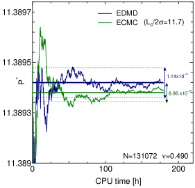
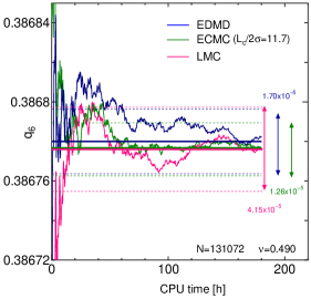
Figure 1: Pressure $P^{*}$ (left) and local order parameter $q_{6}$ (right) in the dense liquid at $\nu=0.490$, obtained from ECMC and EDMD for $N=131,072$ hard spheres. In ECMC, the pressure is computed using the excess displacement method of Eq. (2). In the right panel, the local order parameter of LMC is also shown.

II Model, algorithms, and observables

We consider $N$ monodisperse hard spheres of radius $\sigma$ in a cubic box of sides $L$ with periodic boundary conditions (PBC). The density (packing fraction) $\nu$ is given by $\nu=4/3N\pi\sigma^{3}/L^{3}$. We concentrate on melting and crystallization from the unstable to the stable phase, i.e., from the unstable crystalline branch to the liquid and from the unstable liquid branch to the crystal. For our melting runs, at density $\nu=0.490$ below the coexistence interval of liquid and solid phases, we prepare the initial configurations as perfect fcc crystals, corresponding to the stable phase at high densities (the free energy difference between fcc and hcp crystal have been discussed actively since the works of Ref. woodcock_1997 ; bolhuis_1997 ). The fcc initial conditions are compatible with the cubic simulation box.

For the crystallization runs at density $\nu=0.548$ above the coexistence interval, we start from a fluid initial configuration at a liquid-phase density $\nu=0.490$. In order to reach the higher target density, we repeatedly increase $\sigma$ slightly and remove all created overlaps by sliding overlapping pairs of spheres for a half length of overlap along their common symmetry axis. This is done until all pair overlaps have disappeared.

In EDMD, hard spheres evolve in continuous physical time through collisions, and the dynamics solves Newton’s classical equations of motion. We use an efficient sequential implementation isobe_1999 . LMC and ECMC are implemented very simply. For the former, the optimal displacement of spheres is determined by short LMC runs from the initial conditions so that the acceptance ratio is 1/2. For the latter, a single parameter, the chain length $L_{c}$, must be optimized for each density. A single event can be implemented very quickly in ECMC, as the motion is always in +x or +y, which decreases the CPU time per event. We consider systems with $N=2,048$, $131,072$ and $1,048,576$ spheres. Our calculations are mainly done on the Intel Xeon CPU E5-2680 2.80GHz, where we reach $\sim 3.15\times 10^{9}$ events/h of CPU time for ECMC and $\sim 4.62\times 10^{8}$ collisions/h for EDMD. For the LMC algorithm, $\sim 6.5\times 10^{9}$ trials/h are reached. All our comparisons of algorithms are in terms of CPU time. To be as fair as possible, the three algorithms were implemented following unified design principles. Furthermore, we used the same computer, the same language (Intel FORTRAN), and the same optimal option of compiler. An event-count would have produced similar results.

We track the time-evolution of the ordering/disordering of the system from the pressure and the local and global orientational order parameters. In EDMD, the nondimensional virial pressure is computed from the collision rate via the virial theorem:

$$P^{*}=\beta P(2\sigma)^{3}=\frac{6\nu}{\pi}\left[1-\frac{\beta m}{3T}\frac{1}{N}\sum_{\rm collisions}b_{ij}\right],$$ (1)

where $T$ is the total simulation time, and $\beta=1/m\left<v_{x}^{2}\right>$ is the inverse kinetic temperature (mass $m$ and mean-square $x$-component of velocity of spheres). The collision force $b_{ij}={\bf r}_{ij}\cdot{\bf v}_{ij}$ is defined between the relative positions and the relative velocities of the collision partners engel_2013 ; erpenbeck_1977 . In ECMC, the pressure $P^{*}$ can be evaluated from the mean excess chain displacement michel_2014 :

$$P^{*}=\frac{6\nu}{\pi}\left<\frac{x_{\text{final}}-x_{\text{initial}}}{L_{c}}\right>_{\text{chains}},$$ (2)

where $x_{\text{final}}$ and $x_{\text{initial}}$ are final and initial positions of each chain, respectively, taking into account the PBC. This convenient formula replaces the tedious extrapolation of the pair correlation function at contact $g_{2}(r=2\sigma)$ that was used previously and that must still be used for LMC. The comparison of the evolving pressure of EDMD (using Eq. (1)) and ECMC (using Eq. (2) in the liquid state at $\nu=0.490$ is shown in the left of Fig. 1. The pressures fluctuate around $P^{*}=11.3893$, and agree within very tight error bars.

Besides the pressure, we quantify the speed of melting and of crystallization via the time-dependent local $q_{6}$ and global $Q_{6}$ order parameters steinhardt_1983 :

$$q_{6} = \frac{1}{N}\sum_{i=1}^{N}\sqrt{\frac{4\pi}{13}\sum_{m=-6}^{m=6}\left|\frac{1}{n(i)}\sum_{j=1}^{n(i)}Y_{6,m}({\bf r}_{ij})\right|^{2}},$$ (3)

$$Q_{6} = \sqrt{\frac{4\pi}{13}\sum_{m=-6}^{m=6}\left|\frac{1}{Nn(i)}\sum_{i=1}^{N}\sum_{j=1}^{n(i)}Y_{6,m}({\bf r}_{ij})\right|^{2}},$$ (4)

where $n(i)$ is the number of nearest neighbors for each sphere $i$ and $Y_{6,m}({\bf r}_{ij})$ are the spherical harmonics with icosahedral symmetry for the distance vector ${\bf r}_{ij}$ between spheres $i$ and $j$. We detect nearest neighbors by the SANN algorithm of Meel et al.meel_2012 rather than by the Voronoi construction. On the right of Fig. 1, we again demonstrate that the equilibrium values for $q_{6}(\sim 0.38678)$ agree within tight error bars for LMC, ECMC and EDMD. Similar agreement was reached for the global order parameter $Q_{6}$. We note that perfect fcc configurations have an orientational order $Q_{6}=q_{6}\sim 0.575$, while for liquid configurations (including our disordered initial configurations) $Q_{6}$ approaches zero. In the dense liquid, the local order $q_{6}$ is non-zero because of the build-up of transient local crystal structures isobe_2012 .

III Results

III.1 Hard-sphere phase diagram

Figure 2: Hard-sphere equation of state obtained by ECMC after $\sim{\cal O}(10^{12})$ collisions. The snapshots in the coexistence interval at $N=1,048,576$ represent the local orientational order $q_{6}(i)$ for each sphere $i$ (liquid-like local order is represented in green - solid-like local order in blue). The equilibrium coexistence pressure for the infinite system is also shown. The densities $\nu=0.490$ and $\nu=0.548$, on which we concentrate in Sections III.2 and III.3, are indicated.

The fluid-solid coexistence in the $NVE$ ensemble (which, for hard spheres, corresponds to the common $NVT$ ensemble) for densities $\nu$ in the interval $0.494<\nu<0.545$ has been investigated for more than 50 years alder_1957 ; wood_1957 ; alder_1968 .

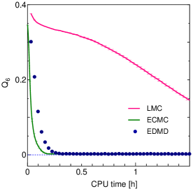
Figure 3: Melting at $\nu=0.490$ ($N=131,072$) from an fcc initial configuration into the stable liquid, tracked by the time evolution of the global $Q_{6}$ order parameter in LMC, EDMD, and ECMC with optimal chain length ($L_{c}/2\sigma=5.87$). Data averaged over 5 samples. Note that ECMC and EDMD are orders of magnitude faster than LMC.

Recently, various theoretical equations of states were compared with the results of a large-scale EDMD simulation on this system, bannerman_2010 with $N\sim 10^{6}$. The metastable fluid branch in the fluid-solid coexistence window was found stable against freezing on EDMD time scales up to $\sim{\cal O}(10^{9})$ collisions. To speed up the simulation, the replica exchange MC method was adapted to the hard-sphere case. To keep the acceptance rate at reasonable values, many replicas at finely spaced densities had to be used, and this approach proved restricted to quite small system sizes ($N=32$ and $N=108$). odriozola_2009 Fernandez et al. fernandez_2012 explored the coexistence of hard-sphere systems in equilibrium by tethered MC for relatively small system sizes $\sim{\cal O}(10^{3})$. In this method, the approach to equilibrium is accelerated by a biased field of two order parameters. The equilibrium pressure $P^{*}=11.5727(10)$ is obtained through extrapolation towards the infinite-size limit. We note that in three-dimensional hard spheres, the direct simulation remains difficult in the coexistence region, even for ECMC, whereas for the analogous two-dimensional hard disks, the equilibration of the coexisting hexatic and liquid phases by ECMC proved possible at all densities, for up to one million disks.bernard_2011

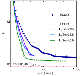
Figure 4: Crystallization at $\nu=0.548$ from a random initial configuration, tracked by the evolution of the pressure $P^{*}$ in EDMD and ECMC with different chain lengths $L_{c}$. Data averaged over $100$ samples for $N=131,072$ (left) and $5$ samples for $N=1,048,576$ (right). The inset in the left panel illustrates the influence of the parameter $L_{c}$ on the performance of ECMC.

Fig. 2 shows the hard-sphere equation of state from ECMC (final pressures after long runs with ($2\sim 3\times 10^{12}$) collisions). The pressure is averaged over $10^{10}$ collisions at the end of the simulation. The stable and unstable fluid pressures well agree with Hoover-Ree hoover_1968 and Carnahan-Starling extrapolation. carnahan_1969 Inside the coexistence interval, the final pressure depends on the initial configuration, as the metastable fcc solid or fluid initial configurations are preserved on the time-scale of the simulation. In the $NVE$ ensemble, the presence of interfaces of different topologies makes that the equation of state is non-monotonous, and the liquid-solid coexistence pressure curve is not flat in a finite system. As one increases the density from the liquid phase, the spherical or cylindrical droplets that can be seen in Fig. 2 generate an excess Laplace pressure. This is analogous to what was found in two-dimensional hard disks bernard_2011 ; mayer_1965 , which show droplets and stripes or in fluid-gas mixtures of the three-dimensional Lennard-Jones system Binder_AmJP , where spherical and cylindrical droplets as well as two-dimensional stripes are found.

Specifically, for $\nu<0.498$, simulations from arbitrary initial conditions converge to the same pressure since the system is completely liquid and nucleation barriers are low. In the region of $\nu=0.500\sim 0.514$, simulations from fcc initial configurations successfully create interfaces with different topologies, whereas simulations from fluid initial conditions remain on the fluid branch. The pressure at $\nu=0.498\sim 0.514$ decreases as $P^{*}=12.2\sim 11.5$, and agrees with the expected coexistence pressure. fernandez_2012 The phase coexistence at equilibrium can be seen clearly by the spatial distributions of the local $q_{6}$ order parameter, where the fcc crystal reduces to a droplet ($\nu=0.500\sim 0.502$) when started from an fcc crystal. For larger densities ($\nu=0.504\sim 0.512$) the remaining fcc phase has the form of a cylinder that reconnects through the PBC, surrounded by the liquid dominant phase created through melting (see the insets of Fig. 2). In the density interval $\nu=0.514\sim 0.530$, the fcc crystal and the liquid remain metastable on the available scales of simulation time. For $\nu=0.532\sim 0.543$, simulations from fluid initial conditions nucleate fcc droplets. At $\nu>0.543$, simulations from fluid initial condition drop down near the solid branch, however, relaxation is in progress at the value around slightly higher pressure than the solid branch, except for the case of $N=2,048$.

III.2 Melting from an fcc initial configuration at a fluid density

We now study the speed of melting into the equilibrium liquid phase at $\nu=0.490$ from an fcc crystalline initial configuration for $N=131,072$. From the global order parameter $Q_{6}$, as shown in Fig. 3, the initial fcc configuration ($Q_{6}\sim 0.575$) rapidly becomes unstable for the three algorithms and approaches the liquid branch, where the global orientational order approaches zero. Melting is much faster for ECMC and EDMD than for LMC. ECMC is found to be somewhat faster than EDMD.

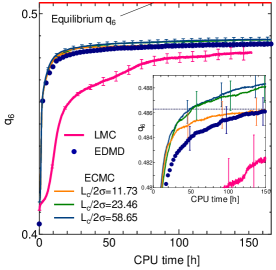
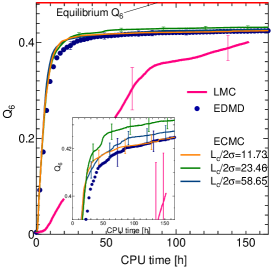
Figure 5: Crystallization at $\nu=0.548$ from a fluid initial configuration with $N=131,072$, tracked by the evolution of local $q_{6}$ and global $Q_{6}$ order parameters by LMC, EDMD and ECMC with different chain lengths $L_{c}$. Data averaged over $100$ samples.

III.3 Crystallization from a fluid initial condition at a solid density

In Fig. 4, we show the evolution toward crystallization of EDMD and of ECMC with different chain lengths $L_{c}$. Results are averaged over $100$ samples for $N=131,072$ (left of Fig. 4) and over $5$ samples for $N=1,048,576$ (right of Fig. 4). Results for three trial runs in which we changed the chain length $L_{c}$ are also shown Fig. 4. The efficiency of ECMC naturally depends on $L_{c}$. For both methods, the pressure remains somewhat above the configurational equilibrium pressure $P^{*}\sim 11.934$. The relative advantage of ECMC with optimal chain length is evident.

In Fig. 5 and Fig. 6, we show the evolution of the local $q_{6}$ and global $Q_{6}$ order parameters in crystallization runs of EDMD and ECMC with three chain lengths. The number of samples is again $100$ for $N=131,072$ and $5$ for $N=1,048,576$. In the early stage of relaxation, $q_{6}$ and $Q_{6}$ are increasing functions of CPU time. In the perfect fcc configuration, the local and global order parameters agree to $q_{6}=Q_{6}=0.57452$. Due to thermal fluctuations, actual numerical simulation at fcc equilibrium estimate the order parameters to $(q_{6},Q_{6})=(0.505,0.483)$ in $(N,\nu)=(1,048,576,0.548)$. Although the crystallization still proceeds, our final averaged $q_{6}$ and $Q_{6}$ reach around $0.488$ and $0.432$, respectively. The inconsistency between the fcc crystal structure and the (finite) simulation box may well be responsible for the reduction in order parameter.

Order parameters decay towards higher order in time, ECMC with optimal chain length $L_{c}/(2\sigma)=23.46$ needs $48.6$ CPU hours to reach at $q_{6}=0.4863$ in $N=131,072$, however, EDMD needs $165$ CPU hours. Both smaller and larger $L_{c}$ results in the inefficiency of relaxation. After $165$ hours, one quarter of ECMC simulations had almost reached the equilibrium state (i.e, $q_{6}>0.99\times{q_{6}}_{eq.}$) whereas for EDMD, only $10$ % had reached such values. The results for LMC are also shown in Fig. 5, and they show that it is much slower than ECMC and EDMD. For example, our LMC simulation on average reaches $q_{6}=48.25$ after ${\cal O}(10^{7})$ LMC sweeps corresponding to $152$ CPU hours. At this $q_{6}=48.25$, ECMC and EDMD needs only about $11$ and $28$ CPU hours, respectively. The decay of $Q_{6}$ has the same tendency as that of $q_{6}$, however, its values are lower than that of $q_{6}$. Since the whole system is slower to order than to establish local order, the global orientation also grows more slowly than the local orientation. In the larger case $N=1,048,576$, ECMC with optimized chain length and EDMD need $416$ and $1,000$ CPU hours to reach $q_{6}=0.4897$, respectively. Note that if chain length is not optimized, the performance of ECMC changes drastically and becomes comparable to or slower than that of EDMD. As for $q_{6}$ and $Q_{6}$, ECMC with optimal length is faster than that of EDMD for a certain factor depending on the target point, which will be discussed in Section III.4.

III.4 Relative Speed of ECMC and EDMD

To further quantify the equilibration speed of ECMC and EDMD, rather than the observables as a function of time ${\cal O}(t)$, we consider the elapsed CPU time ${\cal T}({\cal O})$ from the beginning of the simulation $t=0$ at which the observable ${\cal O}$ is reached. This allows us to define the relative efficiency $R_{s}$:

$$R_{s}({\cal O})={\cal T}_{\rm EDMD}({\cal O})/{\cal T}_{\rm ECMC}({\cal O}),$$ (5)

and analogously for any pair of algorithms, where ${\cal O}$ is an observable, in our case the pressure $P^{*}$, or the local and global order parameters $q_{6}$ and $Q_{6}$.

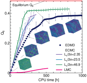
Figure 6: Crystallization at $\nu=0.548$ from a random initial configuration with $N=1,048,576$ tracked by the evolution of local $q_{6}$ and global $Q_{6}$ order parameters in LMC, EDMD and ECMC with different chain lengths $L_{c}$. Data averaged over $5$ samples. Note that LMC is much slower than the other two methods.

For the melting case (not shown) at $\nu=0.490$, $R_{s}$ for observables takes around $3.2$ ($t=0$) to $1$ at the end of simulation. EDMD is slightly slower than that of ECMC. This relative speed remains rather unchanged during the melting process. The situation changes drastically for the crystallization process. Fig. 7 shows $R_{s}$ as a function of normalized observables as $\hat{\cal O}=({\cal O}-{\cal O}_{\text{initial}})/({\cal O}_{\text{equil.}}-{\cal O}_{\text{initial}})$ at $\nu=0.548$ in the crystallization process, at which each data can be estimated by Fig. 4 - Fig. 6. ${\cal O}_{\text{initial}}$ and ${\cal O}_{\text{equil.}}$ are the values at $t=0$ and at the equilibrium, respectively. Those are obtained by independent runs at the perfect fcc crystal which are $q_{6}=0.505$, $Q_{6}=0.483$, and $P^{*}=11.934$. In all cases, $R_{s}({\cal O})$ is increasing function and growing drastically near the crystal (i.e., $\hat{\cal O}>0.8$) as a hockey stick curve. The relative efficiency $R_{s}$ depends rather weakly on system size. We did not compute variations precisely, as the running times ${\cal T}$ were only averaged over 5 samples for $N=1,048,576$. The different algorithmic complexity of our methods might marginally contribute to the size dependence of $R_{s}$: Our EDMD algorithm is implemented in $O(N\log N)$ per $N$ collisions and ECMC as $O(N)$ per $N$ collisions. At $q_{6}=0.47$, $R_{s}(q_{6})$ takes $1.33$ ($N=131,072$) and $1.49$ ($N=1,048,576$), respectively.

IV Conclusion

In this paper, we compared hard-sphere Monte Carlo and Molecular Dynamics algorithms, that coincide in their equilibrium properties. In large systems with up to one million spheres, we recovered the known phase diagram and especially the coexistence region. We quantified the approach towards equilibrium, namely towards the fcc crystal from the liquid-like initial configuration at packing $\nu=0.548$ or the stable liquid from an fcc initial configuration at packing $\nu=0.490$. We clearly showed that the EDMD and ECMC are orders of magnitude faster than the LMC algorithm for both the melting and the crystallization. ECMC needs optimization for chain length $L_{c}$, and we generally find that the individual chains should wrap a few times around the simulation box. The effect of the chain length is rather drastic, and $L_{c}$ must be optimized carefully. The optimal chain length for the crystallization process is estimated around $L_{c}/(2\sigma)\sim 25$ ($N=131,072$) and $50$ ($N=1,048,576$). With a fixed $L_{c}/(2\sigma)$, the actual chain length $\left<x_{\text{final}}-x_{\text{initial}}\right>/(2\sigma)$ can be obtained by trial and error before the production runs. It may also be estimated by the ECMC pressure formula, Eq. (2)), as

$$\frac{\left<x_{\text{final}}-x_{\text{initial}}\right>}{2\sigma}=\frac{P^{*}(L_{c}/(2\sigma))\pi}{6\nu}.$$ (6)

which is evolving during simulation according to pressure relaxation. In case of the optimal chain length $L_{c}/2\sigma=23.46\sim L_{x}/2$, the chain winds around $6$ times around the periodic box. While doing so, very few spheres get hit more than once.

We conclude that ECMC with well-chosen chain lengths is far superior to LMC, although it can be implemented just as easily kapfer_2013 ; kampmann_2015 . Even with respect to molecular dynamics, it performs very well. The clearest advantage of ECMC over EDMD shows up in the crystallization, that is, in the buildup of long-range correlations. We expect the ECMC algorithm and its extension to continuous potentials to be helpful to investigate jamming and to estimate accurate nucleation rate filion_2010 ; auer_2001 and to analyze the full scenario of nucleation and precursor crystallization granasy_2014 . Of particular interest might be that ECMC remains event-driven even for continuous potentials and very simple to implement. Molecular dynamics, on the other hand, must be implemented as a time-driven algorithm for continuous potentials. The discretization of the equations of motion then makes molecular dynamics rather awkward to implement.

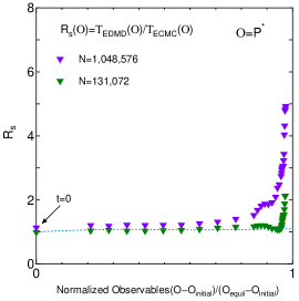
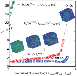
Figure 7: Relative speed $R_{s}$ (see Eq. (5)) of LMC, ECMC and EDMD as a function of normalized observables $\hat{\cal O}=({\cal O}-{\cal O}_{\text{initial}})/({\cal O}_{\text{equil.}}-{\cal O}_{\text{initial}})$, (left) ${\cal O}=P^{*}$ and (right) ${\cal O}=Q_{6}$ for $N=1,048,576$. As also shown in Fig. 6, both ECMC and EDMD are orders of magnitude faster than LMC. ECMC shows considerable advantage over EDMD in the later times of the evolution, when large-scale structures are built up.

- (1) N. Metropolis, A. W. Rosenbluth, M. N. Rosenbluth, A. H. Teller, and E. Teller, J. Chem. Phys. 21, 1087 (1953).
- (2) W. W. Wood and J. D. Jacobson, J. Chem. Phys. 27, 1207 (1957).
- (3) W. Krauth, Statistical Mechanics: Algorithms and Computations (Oxford University Press, Oxford, 2006).
- (4) B. J. Alder and T. E. Wainwright, J. Chem. Phys. 27, 1208 (1957).
- (5) B. J. Alder and T. E. Wainwright, J. Chem. Phys. 31, 459 (1959).
- (6) B. J. Alder and T. E. Wainwright, Phys. Rev. 127, 359 (1962).
- (7) B. J. Alder, W. G. Hoover, and D. A. Young, J. Chem. Phys. 49, 3688 (1968).
- (8) Y. Hiwatari and M. Isobe ed., The 50th Anniversary of the Alder Transition: — Recent Progress on Computational Statistical Physics — (Prog. Theor. Phys. Suppl., 178, Kyoto, 2009).
- (9) E. P. Bernard, W. Krauth, and D. B. Wilson, Phys. Rev. E 80, 056704 (2009).
- (10) M. Isobe, Int. J. Mod. Phys. C 10, 1281 (1999).
- (11) M. Engel, J. A. Anderson, S. C. Glotzer, M. Isobe, E. P. Bernard, and W. Krauth, Phys. Rev. E 87, 042134 (2013).
- (12) E. P. Bernard and W. Krauth, Phys. Rev. E 86, 017701 (2012).
- (13) M. Michel, S. C. Kapfer and W. Krauth, J. Chem. Phys. 140, 054116 (2014).
- (14) S. C. Kapfer and W. Krauth, Phys. Rev. Lett. 114, 035702 (2015).
- (15) L. V. Woodcock, Nature 385, 141 (1997).
- (16) P. B. Bolhuis, D. Frenkel, S. Mau, and D. Huse, Nature 388, 235 (1997).
- (17) J. J. Erpenbeck and W. W. Wood, in Modern Theoretical Chemistry Vol.6, Statistical Mechanics Part B, edited by B.J.Berne (Plenum, New York, 1977), Chap. 1, p. 1.
- (18) P. J. Steinhardt, D. R. Nelson, and M. Ronchetti, Phys. Rev. B 28, 784 (1983).
- (19) J. A. van Meel, L. Fillion, C. Valeriani, and D. Frenkel, J. Chem. Phys. 136, 234107 (2012).
- (20) M. Isobe and B. J. Alder, J. Chem. Phys. 137, 194501 (2012).
- (21) M. N. Bannerman, L. Lue, and L. V. Woodcock, J. Chem. Phys. 132, 084507 (2010).
- (22) G. Odriozola, J. Chem. Phys. 131, 144107 (2009).
- (23) L. A. Fernández, V. Martín-Mayor, B. Seoane, and P. Verrocchio, Phys. Rev. Lett. 108, 165701 (2012).
- (24) E. P. Bernard and W. Krauth, Phys. Rev. Lett. 107, 155704 (2011).
- (25) W. G. Hoover and F. H. Ree, J. Chem. Phys. 49, 3609 (1968).
- (26) N. F. Carnahan and K. E. Starling, J. Chem. Phys. 51, 635 (1969).
- (27) J. E. Mayer and W. W. Wood, J. Chem. Phys. 42, 4268 (1965).
- (28) K. Binder, B. J. Block, P. Virnau, and A. Troester, Am. J. Phys. 80, 1099 (2012).
- (29) S. C. Kapfer and W. Krauth, J. Phys.: Conf. Ser. 454, 012031 (2013).
- (30) T. A. Kampmann, H. H. Boltz, and J. Kierfeld, J. Comp. Phys. 281, 864 (2015).
- (31) L. Filion, M. Hermes, R. Ni, and M. Dijkstra, J. Chem. Phys. 133, 244155 (2010).
- (32) S. Auer and D. Frenkel, Nature 409, 1020 (2001).
- (33) L. Gránásy and G. I. Tóth, Nature Physics 10, 12 (2014).