Mean maps for cosmic web structures in cosmological initial conditions

Abstract

Halos, filaments, sheets and voids in the cosmic web can be defined in terms of the eigenvalues of the smoothed shear tensor and a threshold $\lambda_{\rm th}$. Using analytic methods, we construct mean maps centered on these types of structures for Gaussian random fields corresponding to cosmological initial conditions. Each map also requires a choice of shear at the origin; we consider three possibilities. We find characteristic sizes, shapes and other properties of the central objects in these mean maps and explore how these properties change with varying the threshold and smoothing scale, i.e. varying the separation of the cosmic web into different kinds of components. The mean maps become increasingly complex as the threshold $\lambda_{\rm th}$ decreases to zero. We also describe scatter around these mean maps, subtleties which can arise in their construction, and some comparisons between halos in the maps and collapsed halos at final times.

1 Introduction

The web of cosmological large scale structure is both strikingly evident in observations and simulations and difficult to characterize. Its existence has been known for several decades (Zel’dovich, Einasto & Shandarin, 1982; Shandarin & Zel’dovich, 1983; Einasto et al., 1984; Bond, Kofman & Pogosyan, 1996), and a huge number of different approaches have been used to study it since. Recent overviews of many of these directions can be found in the Proceedings of the Tallinn conference (2014).

These cosmological structures evolved via gravitational instability from initial conditions which have been characterized by measurements of the cosmic microwave background (e.g., Planck Collaboration (2013)). These early time initial conditions are well described by Gaussian random fields, which can also be classified into cosmic web structures. An assortment of different approximate methods can be used to estimate properties of the late time counterparts of the structures found in the initial conditions. Properties include the fraction of mass which will collapse into a certain type of cosmological structure, the number of such structures, etc. Classic works include Press & Schechter (1974); Bardeen, Bond, Kaiser & Szalay (1986); some textbook descriptions are found in Peacock (1998) and Mo, van den Bosch & White (2010). For instance, peaks in the initial conditions can be associated with collapsed halos at late times on average (Kaiser, 1984), and properties of the peaks can be connected to final time properties of the halos (for instance by tracing back particles in simulations to their early time configurations such as in, e.g., Dalal, White, Bond & Shirokov (2008); Robertson, et al (2009); Ludlow and Porciani (2011); Elia, Ludlow & Porciani (2012); Despali, Tormen & Sheth (2013); Borzyszkowski, Ludlow & Porciani (2014); Ludlow, Borzyszkowski & Porciani (2014)). Halos are the most studied cosmological structures, in part due to their close identification to galaxies (Blumenthal, Faber, Primack & Rees, 1984).

This note extends studies of cosmic structures within the specific cosmic web classification considered in Alonso, Eardley & Peacock (2014). (Their detailed particular definitions are in §2 below.) In that work, they compared analytic predictions for initial random Gaussian fields (equivalently, their values linearly extrapolated to final time) and measurements of fully evolved dark matter simulations at late times (redshift $z=0.1$). For some values of their parameters, including the primary one which we focus upon in this work, the volume fractions of the structures for Gaussian random fields and structures for fully evolved dark matter simulations counterparts at late times were comparable. The analytic mass fractions followed the same trends as found in the final time simulations, but were somewhat too high for sheets and too low for filaments. (Halos, which have the largest overdensities and thus might be expected to have the largest differences in the two methods, contribute a very small fraction to both the mass and volume fractions in this structure classification.)

This analytic classification of cosmological Gaussian initial conditions has further consequences, as the power spectrum also determines mean spatial properties around a given central point. We analyze these spatial properties in this note. We find mean properties of regions around different choices of origin, classified as halos, filaments, or sheets, regions we call mean halos, mean filaments and mean sheets. (The boundary around a “mean void” is more challenging to define as for many parameter choices the mean background is also a void, so that a boundary is not evident). The central shear values of these mean objects are an additional parameter which must be chosen. We explore three natural choices for these mean object central shear values, and measure sizes, shapes, shear profiles, and mean linearly extrapolated overdensities of the resulting mean halos, filaments and sheets. We also discuss scatter around these mean configurations, subtleties in their construction, and some possible relations between mean halos and final time collapsed halos. We consider structures in dark matter only.

Background is given in §2: the particular shear-based web classification we use, analytic estimates for average shear in different objects, the construction of mean maps and the measurement of some of their properties. In §3 we consider three choices of central shear, showing mean map examples for different objects and trends in their properties when changing the parameters defining the cosmic web. We also discuss scatter around the mean. In §4 we turn to possible connections of the mean halos to collapsed halos at late times. In §5 we summarize and conclude. The three appendices give details of the calculations (shear, Zel’dovich displacement and scatter), subtleties which arise in some interpretations of one of our construction methods and properties of mean maps corresponding to slightly different constraints at the origin used by Papai and Sheth (2013). The power spectrum used is for a $\Lambda$CDM universe with $(\Omega_{m},\Omega_{b}h^{2},h,\sigma_{8},n)=(0.31,0.022,0.68,0.83,0.96)$ (Planck Collaboration, 2013), calculated with the Eisenstein & Hu (1999) transfer function.

2 Definitions and methods

The cosmic web can be separated into halos (sometimes called nodes), filaments, sheets and voids. We will use the term halo and node interchangeably, as both terms are commonly used for these structures. There are many different web classifications based upon density, morphology, shear and beyond, some of which concentrate on just finding one particular type of structure (e.g. halos or voids) and others which classify an entire map. We use a classification of the latter sort, assigning a type of cosmic structure to every region based upon its shear.

2.1 Shear

We begin with details of our shear definition and classification. We follow Desjacques and Smith (2008); Papai and Sheth (2013) for definitions and for much of the analysis methodology below. The shear is defined on the initial Gaussian perturbations as

$$\xi_{ij}({\bf r})=\frac{1}{\sigma}\partial_{i}\partial_{j}\Phi({\bf r})\;.$$ (1)

Our potential $\Phi({\bf r})$ has the same spatial dependence as the Newtonian potential $\phi$ at early times but is time independent: $\Phi({\bf r})=\phi({\bf r},a)/4\pi Ga^{2}{\rho}_{b}D(a)$. Here $G$ is Newton’s constant, $\rho_{b}$ is the mean background density of the universe, and $D(a)$ is the linear growth factor describing how linear structure grows as the universe expands with scale factor $a$. The derivatives $\partial_{i}$ are with respect to the comoving coordinates ${\bf r}$. The potential $\Phi({\bf r})$ is related to the initial density perturbations evolved linearly to the present time, $\delta({\bf r})$, via the Poisson equation:

$$\sum_{i}\partial_{i}^{2}\Phi({\bf r})=\delta({\bf r})\;\;.$$ (2)

At times earlier than the present time the linearly evolved overdensity obeys

$$\delta_{L}({\bf r},a)=D(a)\delta({\bf r})\;.$$ (3)

The linearly evolved overdensity at the present time, $\delta({\bf r})$ at position ${\bf r}$ is defined in terms of (the linearly evolved to the present time) density via $\rho({\bf r})/\bar{\rho}-1$.

The factor $\sigma$ is the square root of the integral of the power spectrum $P(k)$ associated with $\delta({\bf r})$, smoothed on scale $R_{s}$

$$\sigma^{2}=\frac{1}{2\pi^{2}}\int dkk^{2}P(k)W_{R_{s}}^{2}(k)\;,$$ (4)

i.e., the root mean square fluctuations of the density contrast $\delta({\bf r})$. We use a Gaussian window function,

$$W_{R_{s}}(k)=e^{-\frac{1}{2}(kR_{s})^{2}}\;,$$ (5)

in part to connect more closely with Alonso, Eardley & Peacock (2014), as we use their parameters as a starting point below. One of the parameters of the classification is the smoothing scale $R_{s}$. We will show results from $R_{s}=4h^{-1}Mpc$, studied in depth by Alonso, Eardley & Peacock (2014), but note trends we saw for other cases we explored, $R_{s}=(0.5,1,2,8.9,10,19)\;h^{-1}Mpc$.

Again, to make the notation clear, because $D(a=1)=1$, $\delta({\bf r})$ equals the linearly evolved density perturbation today and $\sigma$ corresponds to its commonly used definition as the square root of the integral of the power spectrum linearly evolved to the present day. Some other approaches include $D(a)$ in the overdensity, and thus in $\Phi$. As the fluctuations $\sigma$ are associated with the overdensity, in our definition they have a factor of $D(a)$ as well, and so $\xi_{ij}$ remains time independent. This is one reason for introducing $\sigma$ into our definition of shear. Other definitions of shear also sometimes take out the trace, again not the case here. When the shear in numerical simulations is considered, Eq. 1 is often used as well, but with the the fully evolved nonlinear potential (determined by the evolved densities in the simulation), rather than its linearly evolved counterpart used in the analytic work in this note.

The potential $\Phi$ can also be used to find the Zel’dovich approximation to the displacement of initial positions at a later time. In the Lagrangian approach to structure formation, the final position ${\bf x}$ of an initial mass component with initial position ${\bf q}$ is related via the displacement ${\bf\Psi}({\bf q},t)$:

$${\bf x}={\bf q}+{\bf\Psi}({\bf q},t).$$ (6)

In the Zel’dovich approximation,

$${\bf\Psi}^{Z}=D(a)\nabla_{q}\Phi\;.$$ (7)

For the initial configuration, with coordinate ${\bf q}$, multiplying the linear final time density by $D(a)$ and taking $a$ small gives the initial density (which is linear because it is small, $\delta_{L}({\bf r},a)=D(a)\delta({\bf r})\sim 0$ as $a\to 0$ and ${\bf x}\to{\bf q}$).

The shear can thus be thought of either as a property of the linearly evolved final density perturbations, or as a property of positions at early times (which then change, using Eq. 6). We will discuss properties in both interpretations.

2.2 Cosmic web classification

The $3\times 3$ shear matrix $\xi_{ij}$ has three eigenvalues, traditionally ordered as $\lambda_{1}\geq\lambda_{2}\geq\lambda_{3}$. Their sum, the trace of the shear, is proportional to the density by Eq. 2,

$${\rm tr}\;\xi_{ij}=\sum_{i}\lambda_{i}(\bf r)=\frac{1}{\sigma}\delta(\bf r).$$ (8)

Halos, filaments, sheets and voids can then be defined as regions where (3,2,1,0) respectively of the $\lambda_{i}$ are above some threshold $\lambda_{\rm th}$. In one way of estimating later structure formation, an initial region is expected to collapse at late times if it linearly evolves to cross some overdensity threshold $\delta_{c}$. As the linearly evolved overdensity $\delta({\bf r})=\sigma\sum_{i}\lambda_{i}({\bf r})$, and regions classified here as halos might be expected to collapse at late times (this is an assumption), this relation suggests some minimum $\lambda_{i}$, i.e. nonzero $\lambda_{\rm th}$, for initial conditions. Note that this condition also means that the mean background, $\lambda_{i}=0$, is also classified as a void. There are thus two scales in this classification, the smoothing $R_{s}$ and the threshold $\lambda_{\rm th}$. Many different choices have been used in the literature.

The same eigenvalue classification is sometimes used for dark matter simulations, but (as mentioned above) using the shear associated with the fully evolved nonlinear potential, see, e.g., Hahn et al (2007); Forero-Romero et al (2009) and references therein. For example, in dark matter nonlinear simulations evolved to redshift zero, Hahn et al (2007) found $R_{s}=2h^{-1}Mpc$ and $\lambda_{\rm th}=0$ separates structure into these different classes in a way that matches visual estimates, while Forero-Romero et al (2009) considered $R_{s}=0.88h^{-1}Mpc$ and $\lambda_{\rm th}=0,0.2,0.4.,1.,2.$ and found improvements for $\lambda_{\rm th}>0$ based upon volume fractions and mass fractions.

One comparison between the above analytic and simulation approaches is by Alonso, Eardley & Peacock (2014). In both approaches, they measured the mass fraction and volume fraction in the four cosmic structures as a function of $\lambda_{\rm th}$, and for two values of $R_{s}$. They found reasonable correspondence of volume and mass fractions for filaments, sheets and voids between the analytically calculated linearly evolved perturbations and the numerically evolved fully nonlinear simulations. Given this, we looked for further characteristic properties of the cosmic web in the analytic construction and report these properties here. We focus for the most part on the parameters used in Alonso, Eardley & Peacock (2014).

We will use these definitions of halos, filaments, sheets and voids to analytically calculate mean configurations of each, for initial random Gaussian field configurations with different choices of $R_{s}$ and $\lambda_{\rm th}$. Unlike Press-Schechter theory where one changes the smoothing scale to consider different mass halos, here the one smoothing scale produces a separation of a full configuration into halos, filaments, sheets and voids, i.e. one smoothing scale completely classifies an entire map. Our mean objects correspond to one such specific smoothing scale and threshold.

2.3 Average shear eigenvalues

The analytic definition of halos, filaments, sheets and voids in terms of $\lambda_{\rm th}$ allows the calculation of volume and mass fractions in each type of object and the average value of each of the eigenvalues $\lambda_{1},\lambda_{2},\lambda_{3}$ in the Gaussian random field initial conditions.

The probability distribution for the ordered eigenvalues $\lambda_{1}\geq\lambda_{2}\geq\lambda_{3}$ of a Gaussian random field is (Doroshkevich, 1970)

$${p}({\lambda}_{1},{\lambda}_{2},{\lambda}_{3})=\frac{3375}{8\sqrt{5}\pi}e^{-3I_{1}^{2}-\frac{15}{2}I_{2}}({\lambda}_{1}-{\lambda}_{2})({\lambda}_{1}-{\lambda}_{3})({\lambda}_{2}-{\lambda}_{3})$$ (9)

where $I_{1}={\lambda}_{1}+{\lambda}_{2}+{\lambda}_{3}$ and $I_{2}={\lambda}_{1}{\lambda}_{2}+{\lambda}_{2}{\lambda}_{3}+{\lambda}_{1}{\lambda}_{3}$. Note that our $\lambda_{i}$ differ by a factor of $\sigma$ from that in Doroshkevich (1970) because we include $\sigma$ in our definition of shear, Eq. 1. Expressions for pairs of eigenvalues or individual eigenvalues are found in Lee and Shandarin (1998) and another interesting rewriting is in Alonso, Eardley & Peacock (2014).

The probability of the eigenvalues restricted by some condition $C$, given for example in terms of $\lambda_{\rm th}$, is given by

$$P(C)=\int_{C}d^{3}\lambda p(\lambda_{1},\lambda_{2},\lambda_{3})\;.$$ (10)

One case of interest for us is where the shear in the region $C$ obeys the constraints for a halo, filament, sheet or void in terms of $\lambda_{\rm th}$. The mean eigenvalues for this particular constraint $C$, which we will denote by $\bar{\lambda}_{i,CA}$, are

$$\begin{array}[]{l}{\rm halo}\\ {\rm filament}\\ {\rm sheet}\\ {\rm void}\end{array}\left.\begin{array}[]{l}\int_{\lambda_{\rm th}}^{\infty}d\lambda_{1}\int_{\lambda_{\rm th}}^{\lambda_{1}}d\lambda_{2}\int_{\lambda_{\rm th}}^{\lambda_{2}}d\lambda_{3}\\ \int_{\lambda_{\rm th}}^{\infty}d\lambda_{1}\int_{\lambda_{\rm th}}^{\lambda_{1}}d\lambda_{2}\int_{-\infty}^{\lambda_{\rm th}}d\lambda_{3}\\ \int_{\lambda_{\rm th}}^{\infty}d\lambda_{1}\int_{-\infty}^{\lambda_{\rm th}}d\lambda_{2}\int_{-\infty}^{\lambda_{2}}d\lambda_{3}\\ \int_{-\infty}^{\lambda_{\rm th}}d\lambda_{1}\int_{-\infty}^{\lambda_{1}}d\lambda_{2}\int_{-\infty}^{\lambda_{2}}d\lambda_{3}\end{array}\right\}\times p(\lambda_{1},\lambda_{2},\lambda_{3})\frac{\lambda_{i}}{P(C)}\;.$$ (11)

In this example, for each structure the corresponding normalization $P(C)$, Eq. 10, has the same integration limits as the the corresponding integral over $p(\lambda_{1},\lambda_{2},\lambda_{3}){\lambda_{i}}$ (it changes for different structures). For example, for a halo,

$$\bar{\lambda}^{\rm halo}_{i,CA}\equiv\frac{\int_{\lambda_{\rm th}}^{\infty}d\lambda_{1}\int_{\lambda_{\rm th}}^{\lambda_{1}}d\lambda_{2}\int_{\lambda_{\rm th}}^{\lambda_{2}}d\lambda_{3}p(\lambda_{1},\lambda_{2}\lambda_{3})\lambda_{i}}{\int_{\lambda_{\rm th}}^{\infty}d\lambda_{1}\int_{\lambda_{\rm th}}^{\lambda_{1}}d\lambda_{2}\int_{\lambda_{\rm th}}^{\lambda_{2}}d\lambda_{3}p(\lambda_{1},\lambda_{2}\lambda_{3})}$$ (12)

We use the notation $\bar{\lambda}_{i,CA}$ to indicate these constrained averages. It depends both upon $\lambda_{\rm th}$ and the type of structure (halo, filament, sheet or void). In practice, for any given $\lambda_{\rm th}$ we integrated these expressions numerically using mathematica.

Another constraint goes beyond restricting eigenvalues in terms $\lambda_{\rm th}$ for each structure, requiring the $\Phi$ from which they come to also correspond to extremal values of the potential ($\partial_{i}\Phi=0$). In this case the shear obeys conditions to be a halo, filament, sheet or void in terms of $\lambda_{\rm th}$, and its potential also obeys $\partial_{i}\Phi=0$. The measure for the volume average of points obeying this constraint is found in Bardeen, Bond, Kaiser & Szalay (1986), starting with the probability distribution for the random Gaussian fields $\Phi,\partial_{i}\Phi,\xi_{ij}$ times the constraint on $\partial_{i}\Phi$. They were interested in peaks and minima in particular, as their main interest was for halos and voids (they also had a restriction on $\Phi$, which we do not impose here, and thus it drops out of the expressions). Their initial measure for integrating the probability density over volume, shear and $\partial_{i}\Phi$ becomes an integral over the eigenvalues similar to that in Eq. 11, except with an additional measure factor $|\lambda_{1}\lambda_{2}\lambda_{3}|$ (from changing variables in the constraint $\delta_{D}(\partial_{i}\Phi({\bf r}))$ from $\partial_{i}\Phi$ to position and integrating over position).

$$\begin{array}[]{l}\int d^{3}r\int d^{6}\xi\int d^{3}\partial\Phi\delta({\bf r-r_{p}})p(\xi_{ij},\partial_{i}\Phi)\\ =\int d^{3}\lambda\int d^{3}\partial\Phi\delta({\partial\Phi})p({\lambda}_{1},{\lambda}_{2},{\lambda}_{3})|\lambda_{1}\lambda_{2}\lambda_{3}|\;.\end{array}$$ (13)

Here the integral again is over the values of $\lambda_{i}$ obeying the constraint to be a halo, filament, sheet or void. We will call the corresponding average shear values $\bar{\lambda}_{i,{\rm extr}}$. So, for example, for a halo, one has:

$$\bar{\lambda}^{\rm halo}_{i,{\rm extr}}\equiv\frac{\int_{\lambda_{\rm th}}^{\infty}d\lambda_{1}\int_{\lambda_{\rm th}}^{\lambda_{1}}d\lambda_{2}\int_{\lambda_{\rm th}}^{\lambda_{2}}d\lambda_{3}p(\lambda_{1},\lambda_{2}\lambda_{3})|\lambda_{1}\lambda_{2}\lambda_{3}|\lambda_{i}}{\int_{\lambda_{\rm th}}^{\infty}d\lambda_{1}\int_{\lambda_{\rm th}}^{\lambda_{1}}d\lambda_{2}\int_{\lambda_{\rm th}}^{\lambda_{2}}d\lambda_{3}p(\lambda_{1},\lambda_{2}\lambda_{3})|\lambda_{1}\lambda_{2}\lambda_{3}|}$$ (14)

These two kinds of average shear, $\bar{\lambda}_{i,CA}$ and $\bar{\lambda}_{i,{\rm extr}}$, are shown in Fig. 1 below for the 4 kinds of objects, as the dashed and solid lines, and are quite similar.

We will consider one other shear average below, that of the mean objects we construct. The eigenvalues of the average shear within these mean objects will be called $\bar{\lambda}_{i}$.

2.4 Mean shear maps: defining objects and characteristic properties

One can go beyond the analytic volume fractions, mass fractions and the constrained shear eigenvalue averages for each structure type by using the power spectrum. The power spectrum can be used to calculate mean spatial properties of the shear around any given central shear configuration. We make maps of these mean shear values around a given central shear value, and study properties of regions within them, in particular those regions sharing the same cosmic web classification as the central point.

We use the method of Papai and Sheth (2013), following Bardeen, Bond, Kaiser & Szalay (1986), to find the mean values of $\xi_{ij}({\bf r})$ (and thus $\lambda_{i}({\bf r})$) everywhere around a given configuration ${\xi}_{ij}(0)\equiv{\xi}_{ij}$ at the origin. Their calculation, for our case of interest, is summarized in Appendix §A. Denoting the constraint at the origin as $C_{0}$, we thus get a map $\langle\xi_{ij}({\bf r})|C_{0}\rangle$, a mean shear at every point. This shear map depends not only on $C_{0}$ as explicitly indicated, but also upon the linear power spectrum and smoothing. The shear eigenvalues at the origin corresponding to the origin constraint $C_{0}$ are denoted as $\lambda_{i}^{0}$.

Once the mean shear $\langle\xi_{ij}({\bf r})|C_{0}\rangle$ is known everywhere around a given central configuration, a choice of $\lambda_{\rm th}$ separates the mean map into halos, filaments, sheets or voids. If the origin constraint $C_{0}$ corresponds to a halo, the nearest points are usually also halo points, similarly for filaments, sheets and voids. We consider the central objects in the mean maps in the most detail. The central object in a mean map is the region sharing the same cosmic web classification (e.g. filament) as the origin and which are continuously connected to the origin via regions with this same classification. Far away from the origin, the correlations and thus the mean shear go to zero and the mean configuration becomes the mean background (again, this is a void region for $\lambda_{\rm th}>0$). In between the origin and mean background, depending upon parameters, several different types of structures may occur. For instance mean halos tend to have filaments and then sheets around them before reaching the mean background. Similarly, filaments tend to have sheets around them (and sometimes halos within, towards their ends). Voids do not always have a clear boundary because for $\lambda_{\rm th}>0$ they also can include the mean background.

Several quantities can be associated with these resulting mean map objects, such as volume, shape, and average values of shear $\bar{\lambda}_{i}$. All of these depend upon $C_{0}$, $\lambda_{\rm th}$ and $R_{s}$.

We report the volume of these mean objects in terms of the Lagrangian volume for a halo associated with the same window function and smoothing scale $R_{s}$, $V_{\rm halo\;Lag}$. This Lagrangian volume is found by by integrating the background average density at early times (as $\delta_{L}({\bf r},a)\to 0$) against the window function to give $M(R_{s})$ and then converting to $V_{\rm halo\;Lag}=M(R_{s})/\rho_{b}$. For our Gaussian window function, $V_{\rm halo\;Lag}=(2\pi)^{3/2}R_{s}^{3}$. The correspondence between shear and initial Gaussian perturbations means that one can view the volumes of objects in our maps as Lagrangian volumes as well, as their volume also directly gives their mass at early times.

For one choice of shear at the origin, $\lambda_{i}^{0}=\bar{\lambda}_{i,{\rm extr}}$, boundary conditions for the Zel’dovich displacement at the origin are also specified, as $\partial_{i}\Phi=0$. In this case we also calculate the mean linearly extrapolated Lagrangian displacement at late times given by Eq. 7. The mean displacement of the edges of the mean objects gives one way of estimating (using linear evolution) their final size.

An additional measurement we make is of the average of the linearly extrapolated Eulerian overdensity at final time in these mean objects, given by $\langle\delta\rangle=\sigma\sum_{i}\bar{\lambda}_{i}$. In simulations, this has been measured by running the clock backwards, starting with collapsed halo regions in nonlinear simulations. Particles in the final halo are tagged and then traced back in time, and the average of the shears of these particles in the initial conditions is used to calculate the linearly extrapolated Eulerian overdensity at final times. Despali, Tormen & Sheth (2013) found for lower final halo masses that on average $\delta_{\rm extrap}\sim\delta_{c}(1+0.2\sigma(R_{s}))$, and Dalal, White, Bond & Shirokov (2008) found similar trends for higher mass halos. We quote overdensities in terms of this reference $\delta_{\rm extrap}$ below.

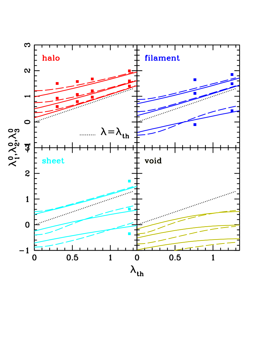
Figure 1: Average values of 3 constrained eigenvalues as a function of threshold $\lambda_{\rm th}$ for each kind of structure. The solid line is $\bar{\lambda}_{i,CA}$ and the dashed line is $\bar{\lambda}_{i,{\rm extr}}$, the dotted line is the threshold $\lambda_{\rm th}$. Eigenvalues for halos (red), filaments (blue), sheets (cyan), and voids (yellow, with black central lines for clarity) are shown at upper left, upper right, lower left, and lower right. These curves are also the central values $\lambda^{0}_{i}$ for two of the three mean map constructions in §3.1, $\lambda^{0}_{i}=\bar{\lambda}_{i,CA}$ for choice 2 and $\lambda^{0}_{i}=\bar{\lambda}_{i,{\rm extr}}$ for choice 3. The filled squares are for choice 1, where $\lambda^{0}_{i}$ is fixed to make the average shear $\bar{\lambda}_{i}$ within the central object satisfies $\bar{\lambda}_{i}=\bar{\lambda}_{i,CA}$. The mean maps hereon use the same colors (for voids, yellow alone) for each kind of structure.

To summarize, for central halo, filament and sheet regions in mean maps we will measure volume, shape (axes lengths), average shear eigenvalues within, $\bar{\lambda}_{i}$, linearly extrapolated average overdensity$\langle\delta\rangle$, and in some cases mean Zel’dovich linearly extrapolated displacement ${\bf\Psi}^{Z}$. Most of our focus is on the objects which include the origin (objects not connected to the origin will be discussed briefly in Appendix §B).

We show examples below of cross sections of these regions along the 3 pairs of spatial axes and of the three shear eigenvalues and linearly extrapolated overdensity along the 3 spatial axes.

3 Shear Map Examples

The mean maps for a given cosmology are determined by the choice of central shear $\langle\xi_{ij}|C_{0}\rangle=(\lambda^{0}_{1},\lambda^{0}_{2},\lambda^{0}_{3})$, the threshold defining the separation into different structures, $\lambda_{\rm th}$, the smoothing $R_{s}$, the window function and the power spectrum. We hold the window function (Gaussian) and power spectrum fixed and show results for $R_{s}=4h^{-1}Mpc$ (commenting on changes for other values). The threshold $\lambda_{\rm th}$ and central shears $C_{0}$ vary as indicated.

3.1 Choices for shear at origin, $\lambda^{0}_{i}$, of mean maps

To construct a mean map, a choice of shear at the origin, $C_{0}$, is required. Mean maps can be constructed for any choice of shear at the origin $C_{0}$, but for a given type of structure and $\lambda_{\rm th}$, we found three choices of particular interest, all motivated by the analytic calculations of average shear given some constraint. Two are associated with $\bar{\lambda}_{i,CA}$, found via Eq. 11, and one with $\bar{\lambda}_{i,{\rm extr}}$, which includes Eq. 13 in the calculation of the average shear eigenvalues. They all yield a value for $\lambda^{0}_{i}$, the shear at the origin as follows (implicitly for choice 1, explicitly for choices 2,3).

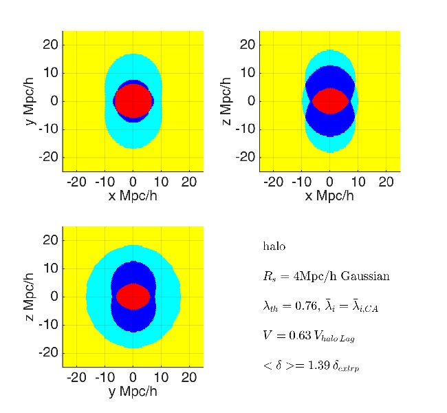
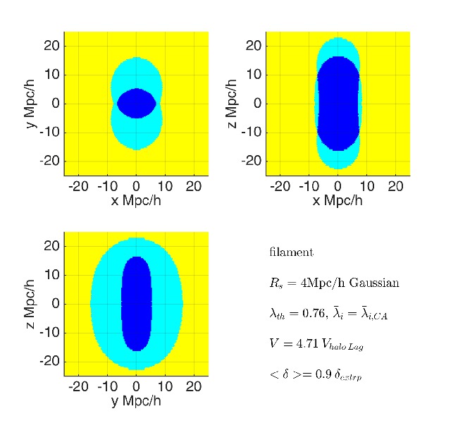
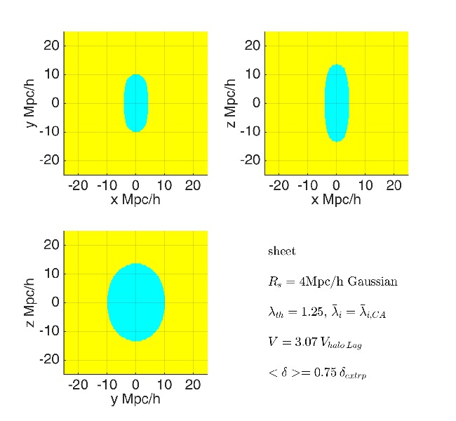
Figure 2: Cross sections of a central mean halo (top left), filament (top right) and sheet (bottom) along three pairs of axes. For each central object, $\lambda^{0}_{i}$ is calculated for the chosen $\lambda_{\rm th}$ (listed in each plot) using choice 1: the average eigenvalues $\bar{\lambda}_{i}=\bar{\lambda}_{i,CA}$ for the corresponding type of structure (halo, filament or sheet). At top left, the mean halo (red) is surrounded by a filament region (dark blue), then a sheet region (cyan) and finally a void (yellow, note mean background is also a “void”). The smoothing $R_{s}=4h^{-1}Mpc$ for all three, the threshold $\lambda_{\rm th}$ is as indicated. The largest eigenvalue is along $x$. For the central object in each, volume and linearly extrapolated overdensity $\langle\delta\rangle$ are also listed. )No mean void is illustrated, as shear corresponding to a void at the origin can smoothly transform to the mean background, which is also a void. It is thus difficult to define the volume of the void and find a central value using this choice, choice 1, for $\lambda^{0}_{i}$.)

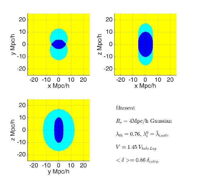
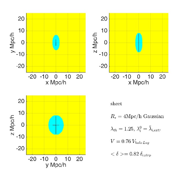
Figure 3: Cross sections analogous Fig. 2, but for central shear $\lambda^{0}_{i}=\bar{\lambda}_{i,{\rm extr}}$ (case 3 in §3.1). Colors, $R_{s}$, and $\lambda_{\rm th}$ as in Fig. 2. In addition, initial edge positions displaced using the mean Zel’dovich approximation, Eq. 7, are connected across the origin via black lines (if they do not go beyond the origin). No mean void is shown as the central configuration smoothly transitions to the mean background, which is also a void.

1.

$\bar{\lambda}_{i}=\bar{\lambda}_{i,CA}$ :
Origin shear choice 1 fixes $\lambda^{0}_{i}$ implicitly, by requiring that the average $\lambda_{i}$ within a particular mean object in the map, $\bar{\lambda}_{i}$, corresponds to $\bar{\lambda}_{i,CA}$ for the corresponding type of structure. That is, the mean object with shear $\lambda^{0}_{i}$ at the origin has average shear corresponding to the average analytic shear, Eq. 11 for that kind of structure. For example, for a halo in the mean map, $\bar{\lambda}^{halo}_{i}=\bar{\lambda}^{\rm halo}_{i,CA}$, where the left hand side is the average over the values in the mean map, and similarly for the corresponding filament (using $\bar{\lambda}^{\rm fil}_{i,CA}$, etc.). In practice, we change the central value of shear until the mean shears within the halo region centered at the origin (which changes in size and shape as the central shear changes), obeys Eq. 12. One possible interpretation is that this gives an “average” such object (e.g. halo), in a smoothed simulation. Practically, we could not always find solutions $\lambda^{0}_{i}$ satisfying the constraint $\bar{\lambda}_{i}=\bar{\lambda}_{i,CA}$ for all $\lambda_{\rm th}$ and all structures, in addition, other complications in this implicit definition can arise (Appendix §B). Our examples below are in the regime where the associated corrections from these possible complications seem small enough to be ignored and where we could find solutions.

2.

${\lambda}^{0}_{i}=\bar{\lambda}_{i,CA}$ :
Origin shear choice 2 sets the central shear $\lambda^{0}_{i}$ equal to the average shear $\bar{\lambda}_{i,CA}$ in Eq. 11 (similar to Papai and Sheth (2013), who used it for long distance properties at final times and whose work inspired this study). This means putting the average shear for a certain structure (for instance a halo) at the origin and then measuring properties of the object made up of the enclosing region of points sharing the same cosmic web classification. In more detail, for a halo, the origin would have shear eigenvalues $\lambda^{0}_{i}=\bar{\lambda}^{\rm halo}_{i,CA}$. Although slightly more complicated to interpret, these maps are much easier to construct, as the central shear is explicitly and immediately calculable. Mean properties around such a point might be interpreted as mean properties around an average point in the corresponding structures in a large map, rather than properties around the central point of a structure (i.e. the peak of a halo does not have average halo properties).

3.

${\lambda}^{0}_{i}=\bar{\lambda}_{i,extr}$ :
Origin shear choice 3 is the volume average of shears obeying some particular cosmic web constraint where in addition $\Phi$ is at an extrema, i.e. where $\partial_{i}\Phi=0$ for all $i$. This is reasonable to expect for a center of a halo or void (minimum or peak) and we can also consider this condition for the center of a filament or sheet. These $\lambda_{i}^{0}=\bar{\lambda}_{i,{\rm extr}}$ are calculated with the extra measure factor derived from Eq. 13. Intuitively, the mean objects corresponding to these central shear values, at least for halos and voids, might correspond to stacking objects in a map, centered on their extremal points (which is often the point used to define the center of such objects).

In Fig. 1 we show the central values for halos, filaments, sheets and voids for these three constructions, as a function of $\lambda_{\rm th}$. As central value 1 required implicit solving of an equation, only a few values are shown, as points (and again, we could not find solutions for all $\lambda_{\rm th}$ in this case, and the construction is ill-defined for voids). The solid line is for case 2, $\lambda^{0}_{i}=\bar{\lambda}_{i,CA}$, the integral in Eq. 11, the dashed line is for case 3, the volume average over extremal points, $\lambda^{0}_{i}=\bar{\lambda}_{i,extr}$. The central values are very similar for the three constructions.

3.2 Mean object cross sections

With these central values we can calculate the mean shear around the origin, and classify each region as halo, filament, sheet, or void. In Fig. 2, we show example cross sections of regions obeying constraint 1 for the central object, i.e. where $\bar{\lambda}_{i}$ within the central object is approximately equal to the corresponding $\bar{\lambda}_{i,CA}$, along the three pairs of axes. We use colors to distinguish between structures: red for halos, dark blue for filaments, cyan for sheets and yellow for voids. The mean background ($\lambda_{i}=0$) is also a void (yellow) for any $\lambda_{\rm th}>0$. (As voids comprise the eventual mean background into which these structures are found, and the majority of the volume, as noted earlier it was not clear how to impose $\bar{\lambda}_{i}=\bar{\lambda}_{i,CA}$ for their case. Thus no void example is shown.) As anticipated, the mean central halo (at top left, Fig. 2) is surrounded by a filament, then a sheet, and then eventually reaches mean density (which is a void), similarly the mean filament (at top right, Fig. 2) is surrounded by a sheet and then void and mean density, and so on. The mean filament does not extend between halos for this value of $\lambda_{\rm th}$ although as $\lambda_{\rm th}$ is lowered halos do eventually appear in the mean filament endpoints. The mean halo has comparable size in all three directions, the filament is extended in one direction compared to the other two, and the sheet has one direction much smaller than the other two, as expected. The larger directions are a few times larger than the smoothing scale $R_{s}$.

Fig. 2 also lists the mean extrapolated overdensity and volume for each central object. (By construction, for choice of origin 1, $\langle\delta\rangle=\sigma\sum_{i}\bar{\lambda}_{i,CA}$.) For the $\lambda_{\rm th}$ and $R_{s}$ here (0.762 and $4h^{-1}Mpc$ respectively), the halo volume is slightly smaller than expected for the Lagrangian region associated with a halo of mass $M(R_{s})$, and the extrapolated density is higher, $V\sim 0.6V_{\rm halo\;Lag},\delta\sim 1.4\delta_{\rm extrap}$.

The change in these quantities using a different choice of $\lambda^{0}_{i}$ can be seen in Fig. 3, where we show mean halo, filament and sheet maps for the same $R_{s}$ and $\lambda_{\rm th}$ values, but choice 3 for shear at the origin, $\lambda^{0}_{i}=\bar{\lambda}_{i,{\rm extr}}$. They are similar to their counterparts in Fig. 2, but slightly smaller, as is expected with their smaller values of $\lambda^{0}_{i}$ (see Fig 1). Choice 3 of shear at the origin also fixes $\partial\Phi=0$ at the origin, implying values for the mean Zel’dovich displacement for points in these structures. In Fig. 3, black lines along each axis connect the position of the initial edges, after they are shifted by their mean Zel’dovich displacements ($\nabla\Phi$). (No line is shown if the displacement crosses the origin. A displacement crossing the origin means that the estimates of the final edge values are well outside of the range of their validity.) Under these displacements, the mean halo contracts and the direction with the largest shear at early times becomes the most contracted at late times, as expected and seen as well in Despali, Tormen & Sheth (2013), see also Ludlow, Borzyszkowski & Porciani (2014); Robles, Dominguez-Tenreiro, Onorbe & Martinez-Serrano (2015). In addition, the mean filament and sheet both contract (only slightly in some directions), while the void, not shown, expands in all directions. As mentioned earlier, the final time estimate for the linear displacement of the initial region edges provides one (very rough) estimate of the mean region’s final size in the Lagrangian picture.

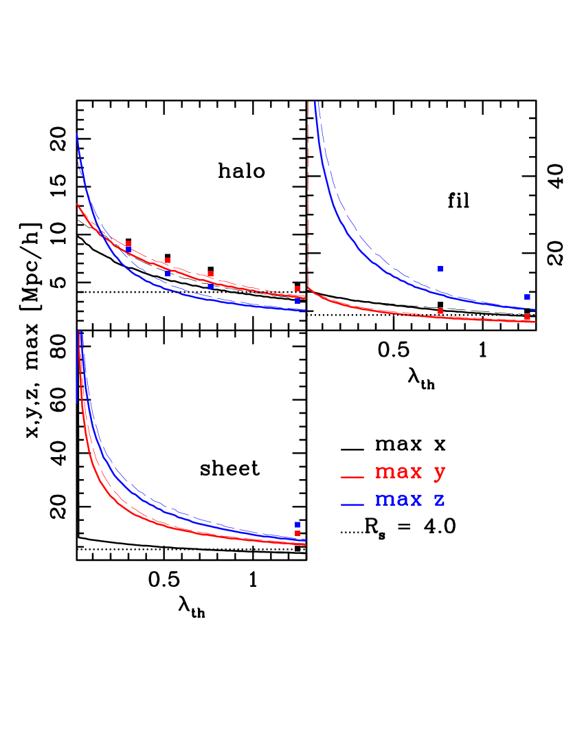
Figure 4: The extent of halos, filaments and sheets, along the $x,y,z$ axes when $\lambda^{0}_{i}=\bar{\lambda}_{i,CA}$ (heavy solid lines) and $\lambda^{0}_{i}=\bar{\lambda}_{i,{\rm extr}}$ (light dashed lines), as a function of $\lambda_{\rm th}$. Filled squares are counterparts for halos, filaments and sheets, at the thresholds shown, when $\bar{\lambda}_{i}=\bar{\lambda}_{i,CA}$, case 1. The smoothing scale $R_{s}=4h^{-1}Mpc$. The largest eigenvalue is along $x$. Examples of objects for case 1 and case 3 are shown in Fig. 2 and Fig. 3 respectively.

More generally, the shapes of the mean objects in these maps as the threshold $\lambda_{\rm th}$ changes can be seen in Fig. 4, for $R_{s}=4h^{-1}Mpc$ and our 3 choices of shear at the origin. (Note that as these are the maximum of each coordinate that the actual filament length is, for instance twice the maximum $z$ value.) Solid points give the extent along the 3 axes for values of $\lambda_{\rm th}$ where we solved choice 1 ($\bar{\lambda}_{i}=\bar{\lambda}_{i,CA}$), solid lines denote choice 2, mean maps centered on $\lambda^{0}_{i}\bar{\lambda}_{i,CA}$, and the lighter dashed lines are for choice 3, $\lambda^{0}_{i}=\bar{\lambda}_{i,{\rm extr}}$. We only sampled central values for condition 1 because it required solving an implicit equation for each $\lambda_{\rm th}$ and each different type of structure, and again, we could not always find a solution.

For a fixed smoothing scale (here $R_{s}$), raising the threshold $\lambda_{\rm th}$ in general raises the average shears within objects, $\bar{\lambda}_{i}$. As can be seen, this simultaneously decreases the volume of the associated mean region for any object beside a void. The shapes of halos, i.e. ratios of extent along different axes, change strongly as the threshold $\lambda_{\rm th}$ varies.

For choice 3 of shear at the origin, the trends of the mean Zel’dovich displacements of the edges of the mean objects could also be studied. We found that the halo edges contract for all $\lambda_{\rm th}$ and that as $\lambda_{\rm th}$ increases the displacements go through the origin and become negative, indicating the approximation is well beyond its range of validity. For filaments and sheets, although 2 or 1 of the edges are/is displaced quickly towards the origin even for small $\lambda_{\rm th}$, for the other edge or edges, as $\lambda_{\rm th}$ increases, the displacement either is small at first (although causing the displaced edge to move towards the origin), or causes the object to first expand (the two larger sheet axes) before again having the displaced edge move towards the origin. The mean Zel’dovich displaced position of the edges divided by the original position of the edges takes roughly the same form for all choices of smoothing we studied.

For many values of $\lambda_{\rm th}$ and $R_{s}$, the mean objects around average points resemble those in Figs. 2,3 above, albeit with different side lengths as just noted. However, as $\lambda_{\rm th}$ tends to zero, not only do central structures get much larger as seen in Fig. 4, but also qualitatively different behavior appears. Cross sections for the case $\lambda_{\rm th}=10^{-4}$ and case 2, $\lambda^{0}_{i}=\bar{\lambda}_{i,CA}$, are shown in Fig. 5. The mean maps are shown for a much larger range of scales, because unlike the two earlier cases shown in Figs. 2,3, where outside the central regions the shear quickly tends to a void, for this low $\lambda_{\rm th}$ non-void structures persist out to large distances. (We consider $\lambda_{\rm th}=10^{-4}$ rather than exactly zero as the functions used to calculate the shears have limited accuracy.) For this threshold, in part because voids and halos only comprise 8% of the total volume each, with sheets and filaments taking 42% each, the structures which are not the mean background (not voids) are extremely large. In addition, unlike Fig. 2, mean filaments have halos within their endpoints, mean sheets have filaments within their outskirts, mean voids have sheets outside of them, and so on, as can be seen. (The presence of halos within the ends of filaments is characteristic of individual filaments in simulations, which are often found by looking for bridges between halos, e.g. Colberg (2007).) Around mean halos, the filaments fan out and do not end within the scales ($\sim 800h^{-1}Mpc$) we consider in 2 directions. Increasing $\lambda_{\rm th}>0$, these extra embedded structures decrease in size and eventually disappear, smoothly transforming into objects similar to those shown in Fig. 2. For $R_{s}=4h^{-1}Mpc$ this transition happens around $\lambda_{\rm th}\sim 0.15$, for $R_{s}=10h^{-1}Mpc$ this happens at an only slightly larger $\lambda_{\rm th}\sim 0.17$. (As might be expected, this rich structure complicates using choice 1 to calculate $\lambda^{0}_{i}$, and is discussed in Appendix §B.) The scatter around this mean configuration is significant as well, as discussed in §3.3 below.

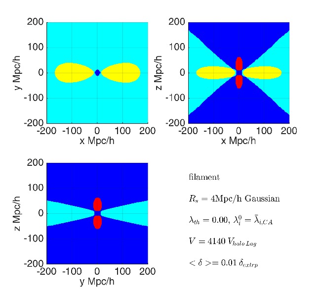
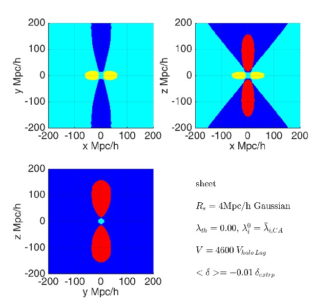
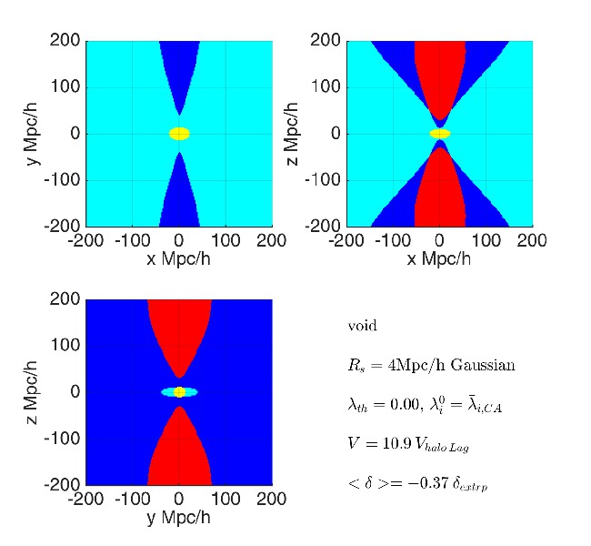
Figure 5: The extreme behavior for $\lambda_{\rm th}=10^{-4}$ of mean regions around $\lambda^{0}_{i}=\bar{\lambda}_{i,CA}$ (case 2) for a halo (top left) filament (top right), sheet (lower left) and void (lower right) for smoothing $R_{s}=4h^{-1}Mpc$. Colors are as in Fig.  2 and Fig. 3. The larger axes scales are used in order to capture the increased volume of non-void structures. The halos in filament edges and filaments in sheet edges visible for this $\lambda_{\rm th}$ decrease as $\lambda_{\rm th}$ increases, eventually disappearing for $\lambda_{\rm th}\sim 0.15$.

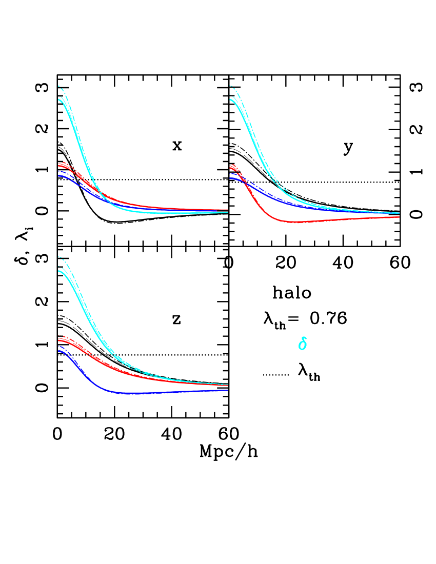
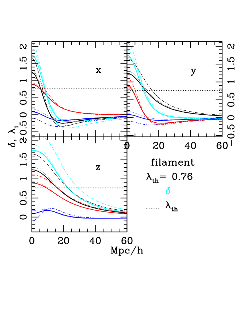
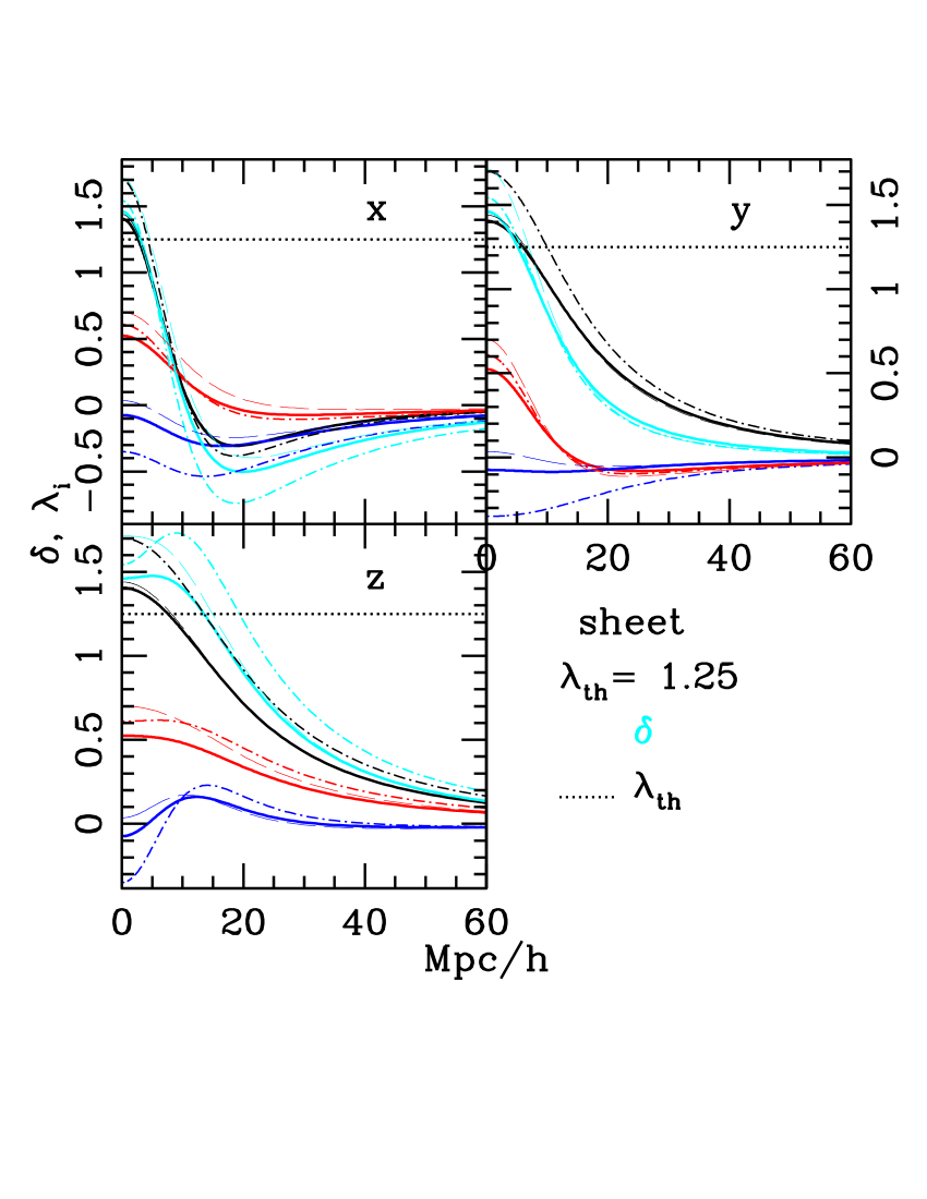
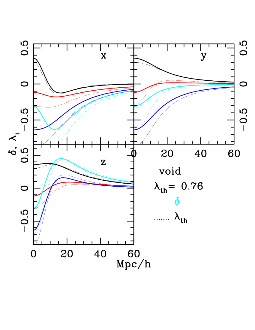
Figure 6: Shear eigenvalue profiles $\lambda_{i}(r)$ (black, blue, red) and linearly extrapolated overdensity $\delta$ (cyan) along $x$,$y$ and $z$ axes, for a halo (upper left panels), filament (upper right panels), sheet (lower left panels) and void (lower right panels). For the $\lambda_{\rm th}$ as in Fig. 2,3 (and $\lambda_{\rm th}=0.762$ for the void), profiles for our three cases of central shear are shown: (1) $\bar{\lambda}_{i}=\bar{\lambda}_{i,CA}$ (medium weight, dot-dashed lines), (2) $\lambda^{0}_{i}=\bar{\lambda}_{i,CA}$ (heavier solid lines) and (3) $\lambda^{0}_{i}=\bar{\lambda}_{i,{\rm extr}}$ (lighter dashed lines). The straight black dotted line is the threshold $\lambda_{\rm th}$ separating out the different structures (not visible for the void example at lower right).

3.3 Mean profiles along axes and scatter

Beyond shape, volume, extrapolated overdensity and mean Zel’dovich displacement of edges of each type of object, one can look at more details of the mean shear itself, for instance the shear values along any given axis. For the mean objects in Figs. 2,3, values along 3 axes for the 3 shear eigenvalues (and the linearly extrapolated overdensity $\delta=\sigma\sum_{i}\lambda_{i}$) are shown in Fig. 6. The dotted straight black line is the threshold $\lambda_{\rm th}$, crossing this means changing structure classificiation (e.g. from a halo to a filament). The profiles for voids with $\lambda^{0}_{i}$ corresponding to central shear choices 2 and 3 ($\lambda_{\rm th}=0.762$) are also shown, as these are explicitly calculable. Central shear choices 1, 2 and 3 correspond to line types dot-dashed, solid and dashed respectively. The different choices of shear at the origin give similar profiles for halos, but the filaments, sheets and voids show some large differences. The void profile, when calculable (i.e. choices 2 and 3 at the origin), has mass compensation at a distance away from the origin in the linearly extrapolated over density as expected. Note that the mean shears take a very long time to approach their eventual value of zero even though they fall below the threshold $\lambda_{\rm th}$ fairly quickly.

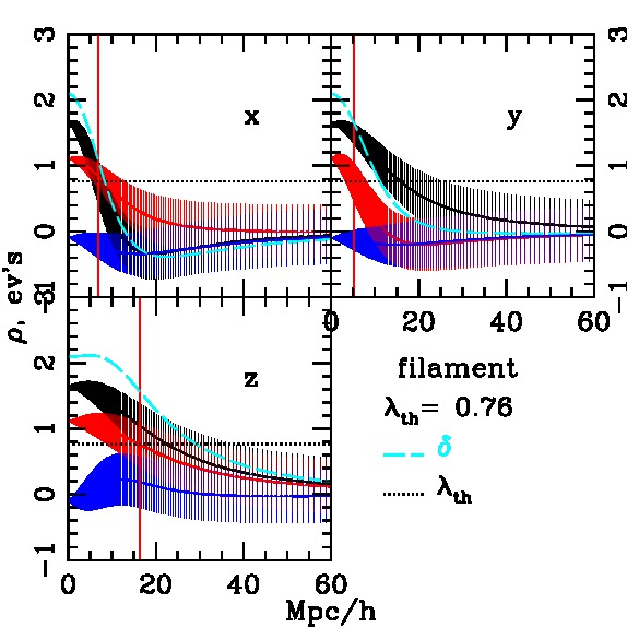
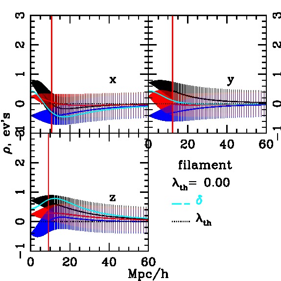
Figure 7: Example of scatter around the mean profiles for a filament with two different central values, $\lambda^{0}_{i}$ set using criterion 1, and $\lambda_{\rm th}=0.762$ at top, using criterion 2 with $\lambda_{\rm th}=10^{-4}$ at bottom. Cross sections for their mean maps are shown in Figs. 2,5 respectively. As a function of distance from the origin, as the smoothing $R_{s}=4h^{-1}Mpc$ for both, the scatter is the same for both examples. However, the effect on the classification of the regions differs because of the difference in the central values due to the difference in threshold $\lambda_{\rm th}$. The solid lines are the shear eigenvalue profiles $\lambda_{i}(r)$ (black, blue, red), and the filled regions show one sigma scatter along $x$, $y$ and $z$ axes. The top filament profile corresponds to the cross sections in Fig. 2 and the profile in Fig. 6, the lower to the filament cross section shown in Fig. 5. The dotted line again is the threshold $\lambda_{\rm th}$. The vertical solid red line is where the mean central filament transitions along that axis to a sheet. For low $\lambda_{\rm th}$, the scatter mixes different structures even at large distances from the origin.

One other scale in the system is the scatter, the variance of the shear around the mean values (calculated in Appendix §A, Eq. 18). The variance depends only on $R_{s}$, the window function, and the position relative to the constrained origin, independent of the central value of the mean configuration and the threshold $\lambda_{\rm th}$. It is simplest to interpret along the 3 axes, where it starts at zero at the origin (where the shear constraint is imposed) and then increases to a constant $\sim$0.2 at a distance $\sim 2R_{s}+1$ for one eigenvalue and at a larger distance, $\sim 4.4R_{s}+5.5$, for the other two. (Calling the matrix in Eq. 18 $C_{ij}$, where $i,j$ are each pairs of indices, the scatter shown is $1/\sqrt{(C^{-1})_{ii}}$ along $i$=11, 22 or 33 respectively.) The effect of this scatter on the classification of a given region depends upon the configuration at the origin and $\lambda_{\rm th}$. We show in Fig. 7 the shear eigenvalue profiles along each of the 3 axes both for the filament case seen in in Fig. 6), and for the filament configuration with $\lambda_{\rm th}\sim 0$, but now also show the envelope of the variance.

In both examples, far from the origin the mean value of shear approaches zero, while the scatter approaches its asymptotic value. At large distances, if $\lambda_{\rm th}$ is high, the configurations close to the mean do not scatter enough to change their classification from a void to anything else. As $\lambda_{\rm th}$ drops, a one-sigma fluctuation will mix many different kinds of structures even at large distances from the origin. Thus, for instance,in Fig. 5 of the cross sections for low $\lambda_{\rm th}$, beyond about 20 $h^{-1}Mpc$, the mean configurations are within one-sigma of all of the structures (e.g., the mean halo is within one-sigma of the mean filament, sheet and void).

Thus the different ways of constructing the mean maps, via different constraints $C_{0}$ at the origin, provide, for the same $\lambda_{\rm th}$, similar objects in size and shape. The mean central objects increase in size and change shape as the threshold $\lambda_{\rm th}$ is decreased, becoming very complicated as the threshold goes to zero. For very small $\lambda_{\rm th}$, the scatter strongly mixes the different structures even far from the origin. The scatter about the mean configurations is independent of the central value and approaches its asymptotic limit at larger distances from the origin as $R_{s}$ increases.

4 Collapsed Halo Interpretation

In general, any smoothing $R_{s}$, and any threshold $\lambda_{\rm th}$ can be used to define halos, filaments, sheets and voids. One can also ask how objects in the smoothed map, such as halos, are related to other ways of defining such objects (e.g. via gravitational collapse at later times).

As halos are the most well studied collapsed objects, we investigated correspondences between our mean halos defined using $\bar{\lambda}_{i}=\bar{\lambda}_{i,CA}$ and final collapsed halos such as are identified in numerical dark matter simulations. Initial conditions for halos and their final properties have been extensively studied in Dalal, White, Bond & Shirokov (2008); Robertson, et al (2009); Ludlow and Porciani (2011); Elia, Ludlow & Porciani (2012); Despali, Tormen & Sheth (2013); Borzyszkowski, Ludlow & Porciani (2014); Ludlow, Borzyszkowski & Porciani (2014). Final collapsed halos can be characterized by their mass and the measured linearly extrapolated overdensity of their initial regions. We checked whether we could find, for each $R_{s}$, a $\lambda_{\rm th}$ such that our mean halo map overdensities matched $\delta_{\rm extrap}(R_{s})$ from Despali, Tormen & Sheth (2013) and $V_{\rm halo\;Lag}=M(R_{s})/\rho_{b}$. We considered all three origin choices in §3.1.They gave similar results: for smaller $R_{s}$, fixing $\langle\delta\rangle$ to the value matching $R_{s}$ gave a $\lambda_{\rm th}$ driven close to zero, or even below, and the Lagrangian volumes were much larger than that associated with $M(R_{s})$, and for larger $R_{s}$ the opposite happened. For $R_{s}=4h^{-1}Mpc$, for cases 1,2,3 respectively we found that $\lambda_{\rm th}=(0.37,0.48,0.43)$ and $V=(2.1,0.57,1.0)M(R_{s})/\rho_{b}$. (This can be compared to the average mass for $R_{s}$ and above at this scale, $M_{+}(R_{s})\sim 1.5M(R_{s})$.) Given the approximations involved and the difficulty in taking into account the higher mass halos, this might be a close enough agreement. In summary, only for one smoothing scale $R_{s}$ did it seem possible to find a $\lambda_{\rm th}$ where the mean halo had its volume close to the Lagrangian volume $M(R_{s})/\rho_{b}$, for our 3 choices of mean object centers.

Initial condition halos do not always give final halos, and not all halos at final times are tagged as halos in the initial conditions, for reasons which have been studied in detail in e.g. Dalal, White, Bond & Shirokov (2008); Robertson, et al (2009); Ludlow and Porciani (2011); Elia, Ludlow & Porciani (2012); Despali, Tormen & Sheth (2013); Borzyszkowski, Ludlow & Porciani (2014); Ludlow, Borzyszkowski & Porciani (2014). For instance, external tidal fields might destroy a initial local peak, or a peak might form at a later time due to a merger.

If we take this choice of threshold as a preferred one for smoothing $R_{s}=4h^{-1}Mpc$, because it gives a better connection to collapsed halos (of one fixed mass) at late times, then we also can consider the characteristic sizes for other objects for this smoothing, from Fig. 4. However, this lack of direct connection to collapsed halos (of one fixed mass) is not necessarily surprising. The mean objects we find for each kind of structure should be more characteristic of the smoothed map than, e.g., for halos, the collapsed objects which can form after full nonlinear evolution.

For modified constraints on both $\lambda_{\rm th}$ and $\delta$ and taking $\lambda^{0}_{i}=\bar{\lambda}_{i,CA}$, Papai and Sheth (2013) compared the analytically predicted density anisotropy at large, i.e. close to linear, distances to that produced by a stack of numerically simulated halos, finding rough agreement. Properties of the mean objects for the origin constraints considered by Papai and Sheth (2013) are given in the Appendix §C.

5 Summary and Discussion

A spatial distribution of Gaussian random fields can be classified into halos, filaments, sheets and voids using a smoothing scale $R_{s}$ and threshold $\lambda_{\rm th}$. These can be associated with linearly evolved initial conditions or with the initial conditions themselves for structure formation. Many smoothing scales and thresholds have been chosen for use in different contexts. The comparison of fractions of volume and mass in the different structures has shown some agreement between analytic calculations of initial Gaussian random fields (specifically their linearly extrapolated values at the present time) and numerical simulations of the full nonlinear evolution (e.g., Alonso, Eardley & Peacock (2014)).

We explored further properties of cosmic structures in the Gaussian random field configurations, for the same classification and parameters used by Alonso, Eardley & Peacock (2014). We used the properties of Gaussian random fields, combined with the power spectrum, to calculate properties of mean halos, filaments, sheets and voids with three choices of central shears $\lambda^{0}_{i}$. These central shears are related either to the mean shears for each type of object, or to the volume average of the extremal shear values for each object. For low $\lambda_{\rm th}$ the mean structures are very complicated, while at larger $\lambda_{\rm th}$ the mean structures centered at the origin smoothly transition to the mean background through the sequence halo to filament to sheet to void. The mean halo has approximately similar extent in all three directions, the mean filament has one larger direction and the mean sheet is small along one direction and larger along the other two. We showed examples of mean structures at large and small $\lambda_{\rm th}$ and discussed trends of their shapes with changes in threshold and in smoothing. One method of choosing the central shear was an implicit condition, which we could not always solve. When the central point is taken to be an extremal point ($\lambda_{i}^{0}=\bar{\lambda}_{i,{\rm extr}}$), there is a natural value for the Zel’dovich displacement at the origin and thus one can also calculate the mean Zel’dovich displacement of the edge points of the mean objects, giving a final linear approximation to the size of each of these objects. For some $\lambda_{\rm th}$, the estimated Zel’dovich change in the mean filaments and sheets is small, while the mean filament and sheets are large relative to the smoothing scale (and sometimes the nonlinear scale), suggesting that these characteristic sizes might persist in the nonlinear maps in some form as well.

We also characterized the scatter around the mean configurations, which tends to a constant at a small multiple of $R_{s}$, the smoothing. The effect of scatter on the classification of structures around the mean background depends in part on $\lambda_{\rm th}$, we showed as an example the scatter for mean filaments for two values of $\lambda_{\rm th}$.

There is not a clear identification of the mean halos with collapsed halos or collapsed halos above some mass. Matching the expected average linearly extrapolated overdensity for a given smoothing $R_{s}$ implies a threshold $\lambda_{\rm th}$, and leads to a Lagrangian volume (final estimated mass) which is too small (large) relative to $M(R_{s})$ for large (small) $R_{s}$, although there might be a sweet spot near $R_{s}\sim 4h^{-1}Mpc$. These estimates were only approximate as different mass definitions are used in the quantities being compared.

As these mean objects are an additional characterization of initial Gaussian random field configurations and smoothed maps, it would be very interesting to compare them to mean objects in simulations with the same smoothing and threshold, both at initial and at late (fully evolved) times. This comparison is nontrivial. Although the division of halo, filament, sheet and void regions is direct in simulations, as are their volume and mass fractions, the separation into specific distinct objects, e.g. different filaments, is not immediate. Splitting halo, filament, sheet and void regions into objects so that their stack gives our mean objects might be a natural way of defining such individual objects in the full map, but presumably additional assumptions will be required. The stacking might be most naturally associated with doing a volume average over extremal points as in our choice 3 of origin shear.

This work is in a different direction than the extremely interesting research on finding the probability distribution of initial conditions which are consistent with a given final measured nonlinear configuration (e.g. the line of study pursued in Jasche, Leclercq & Wandelt (2015); Leclercq, Jasche & Wandelt (2015a, b, c)) although both kinds of studies involve cosmic web classifications of initial conditions and their inferred counterparts at late times.

Several free parameters appeared in the construction, including the threshold $\lambda_{\rm th}$, the smoothing $R_{s}$ and the central values $\lambda^{0}_{i}$. We chose a few different $\lambda^{0}_{i}$, however others are possible. Connections to other natural scales in the initial conditions would be interesting to further pursue as well, such as those discussed in Shandarin (2009) and Pogosyan et al (2009).

JDC thanks J. Peacock, A. Pontzen and J. Whitehouse for suggestions, and especially M. White for numerous discussions. We thank N. Dalal, V. Desjacques, F. Leclercq, M. Neyrinck and the anonymous referee for helpful comments on the draft.

Appendix A Shear calculation details

The mean shear $\langle\xi_{ij}({\bf r})|C_{0}\rangle$ surrounding the origin with fixed boundary conditions $\langle\xi_{ij}|C_{0}\rangle=\lambda^{0}_{i}\delta_{ij}$ can be calculated as described in Papai and Sheth (2013) (based in part upon Bardeen, Bond, Kaiser & Szalay (1986)). Their focus was on $\langle\delta({\bf r})|C_{0}\rangle$, for only one of the boundary conditions $C_{0}$ which we consider, so we give more details for completeness. A more general angle-averaged probability distribution $P(\vec{\xi}(r_{1}),\vec{\xi}(r_{2}),r)$ was found by Desjacques and Smith (2008).

Defining $\vec{\xi}({\bf r})=(\xi_{11}({\bf r}),\xi_{22}({\bf r}),\xi_{33}({\bf r}),\xi_{12}({\bf r}),\xi_{23}({\bf r})$,
$\xi_{13}({\bf r}))$, and $\vec{\xi}\equiv\vec{\xi}(0)$, Papai and Sheth (2013) use the Gaussianity of $p(\vec{\xi}(r)|\vec{\xi})$ to get

$$\langle\vec{\xi}({\bf r})|\vec{\xi}\rangle=\langle\vec{\xi}({\bf r})\vec{\xi}\rangle\langle\vec{\xi}\otimes\vec{\xi}\rangle^{-1}\vec{\xi}\;.$$ (15)

which for conditions $C_{0}$ at the origin then give

$$\langle\vec{\xi}({\bf r})|C_{0}\rangle=\langle\vec{\xi}({\bf r})\vec{\xi}\rangle\langle\vec{\xi}\otimes\vec{\xi}\rangle^{-1}\langle\vec{\xi}|C_{0}\rangle\;.$$ (16)

The Zel’dovich displacement mean value, shown for central shear choice 3 in Fig. 3 can also be calculated analogously to that for $\vec{\xi}({\bf r})$ when the displacement at the origin is fixed to be zero (as it is for choice 3 of central shear):

$$\langle\Psi^{Z}_{i}({\bf r})|C_{0}\rangle=\langle\Psi^{Z}_{i}({\bf r})\vec{\xi}\rangle\langle\vec{\xi}\otimes\vec{\xi}\rangle^{-1}\langle\vec{\xi}|C_{0}\rangle\;.$$ (17)

The variance of $\vec{\xi}({\bf r})-\langle\vec{\xi}({\bf r})|C_{0}\rangle$ is (Bardeen, Bond, Kaiser & Szalay, 1986):

$$\langle\vec{\xi}\otimes\vec{\xi}\rangle-\langle\vec{\xi}({\bf r})\vec{\xi}\rangle\langle\vec{\xi}\otimes\vec{\xi}\rangle^{-1}\langle\vec{\xi}|\vec{\xi}({\bf r})\rangle\;.$$ (18)

which is zero at the origin (where there is a fixed constraint) and then increases, asymptotically reaching $\langle\vec{\xi}\otimes\vec{\xi}\rangle$.

These give the mean value of the shear, Zel’dovich displacement when $\partial_{i}\Phi=0$ at the origin, and scatter at position ${\bf r}$ when the shear at the origin is set by the boundary condition $C_{0}$, which we explore in the body of this paper. The three central shear values $\lambda^{0}_{i}$ which we consider are in §3.1.

To evaluate Eq. 16, Eq. 17 and Eq. 18, we follow Papai and Sheth (2013) in choosing the shear at the origin to be diagonal $\vec{\xi}(0)\equiv\vec{\xi}=\vec{\xi}_{D}=(\xi_{11},\xi_{22},\xi_{33})$, and substitute $\langle\xi_{D}\otimes\xi_{D}\rangle^{-1}$:

$$\begin{array}[]{l}\langle\xi_{ij}({\bf r})|C_{0}\rangle=\\ (6\langle\xi_{ij}({\bf r})\xi_{11}\rangle-3/2\langle\xi_{ij}({\bf r})\xi_{22}\rangle-3/2\langle\xi_{ij}({\bf r})\xi_{33}\rangle)\langle\xi_{11}|C_{0}\rangle\\ +(-3/2\langle\xi_{ij}({\bf r})\xi_{11}\rangle+6\langle\xi_{ij}({\bf r})\xi_{22}\rangle-3/2\langle\xi_{ij}({\bf r})\xi_{33}\rangle)\langle\xi_{22}|C_{0}\rangle\\ +(-3/2\langle\xi_{ij}({\bf r})\xi_{11}\rangle-3/2\langle\xi_{ij}({\bf r})\xi_{22}\rangle+6\langle\xi_{ij}({\bf r})\xi_{33}\rangle)\langle\xi_{33}|C_{0}\rangle\;.\\ \end{array}$$ (19)

The expression for $\Psi^{Z}_{i}$ can be found by replacing $\xi_{ij}({\bf r})$ by $\Psi^{Z}_{i}({\bf r})$.

For the scatter, Eq. 18,

$$\begin{array}[]{l}\langle(\xi_{ij}({\bf r})-\langle\xi_{ij}({\bf r})|C_{0}\rangle)(\xi_{kl}({\bf r})-\langle\xi_{kl}({\bf r})|C_{0}\rangle)\rangle=\\ (6\langle\xi_{ij}({\bf r})\xi_{11}\rangle-3/2\langle\xi_{ij}({\bf r})\xi_{22}\rangle-3/2\langle\xi_{ij}({\bf r})\xi_{33}\rangle)\langle\xi_{11}|\xi_{kl}({\bf r})\rangle\\ +(-3/2\langle\xi_{ij}({\bf r})\xi_{11}\rangle+6\langle\xi_{ij}({\bf r})\xi_{22}\rangle-3/2\langle\xi_{ij}({\bf r})\xi_{33}\rangle)\langle\xi_{22}|\xi_{kl}({\bf r})\rangle\\ +(-3/2\langle\xi_{ij}({\bf r})\xi_{11}\rangle-3/2\langle\xi_{ij}({\bf r})\xi_{22}\rangle+6\langle\xi_{ij}({\bf r})\xi_{33}\rangle)\langle\xi_{33}|\xi_{kl}({\bf r})\rangle\\ +15(\langle\xi_{ij}({\bf r})\xi_{12}\rangle\langle\xi_{12}\xi_{kl}({\bf r})\rangle\\ +\langle\xi_{ij}({\bf r})\xi_{13}\rangle\langle\xi_{13}\xi_{kl}({\bf r})\rangle+\langle\xi_{ij}({\bf r})\xi_{23}\rangle\langle\xi_{23}\xi_{kl}({\bf r})\rangle)\end{array}$$ (20)

This is independent of the value at the origin, and the threshold $\lambda_{\rm th}$.

The correlations $\langle\xi_{ij}({\bf r})\xi_{mm}\rangle$ are

$$\begin{array}[]{ll}\langle\xi_{ij}({\bf r})\xi_{mm}\rangle&=\Psi_{1}(r)\hat{r}_{i}\hat{r}_{j}\hat{r}_{m}^{2}\\ &+\Psi_{3}(r)(2\hat{r}_{i}\hat{r}_{m}\delta_{jm}+2\hat{r}_{j}\hat{r}_{m}\delta_{im}\\ &+\hat{r}_{i}\hat{r}_{j}+\hat{r}_{m}^{2}\delta_{ij})\\ &+\Psi_{5}(r)(\delta_{ij}+2\delta_{im}\delta_{jm})\;,\end{array}$$ (21)

for $mm=11,22,33$, and

$$\frac{1}{\sigma}\langle\Psi^{Z}_{i}({\bf r})\xi_{mn}\rangle=\Psi_{4}(r)\hat{r}_{i}\hat{r}_{m}\hat{r}_{n}+\Psi_{2}(r)(\hat{r}_{i}\delta_{mn}+\hat{r}_{m}\delta_{in}+\hat{r}_{n}\delta_{im})\;.$$ (22)

The basis functions $\Psi_{i}(r)$ depend on the primordial matter power spectrum $\Delta_{\delta}^{2}(k)=k^{3}P_{L}(k)/(2\pi^{2})$. We use a power spectrum for a $\Lambda$CDM universe with $(\Omega_{m},\Omega_{b}h^{2},h,\sigma_{8},n)=(0.31,0.022,0.68,0.83,0.96)$ (Planck Collaboration, 2013), calculated with the Eisenstein & Hu (1999) transfer function. For the $\Psi_{i}(r)$ associated with $\xi_{ij}$ (appendix of Desjacques (2008)),

$$\begin{array}[]{ll}\Psi_{1}(r)&=\frac{1}{\sigma^{2}}\int_{0}^{\infty}d\ln k\Delta_{\delta}^{2}(k)W_{R}(k)^{2}j_{4}(kr)\\ \Psi_{3}(r)&=\frac{1}{\sigma^{2}}\int_{0}^{\infty}d\ln k\Delta_{\delta}^{2}(k)W_{R}(k)^{2}[-\frac{1}{7}j_{2}(kr)-\frac{1}{7}j_{4}(kr)]\\ \Psi_{5}(r)&=\frac{1}{\sigma^{2}}\int_{0}^{\infty}d\ln k\Delta_{\delta}^{2}(k)W_{R}(k)^{2}[\frac{1}{15}j_{0}(kr)\\ &+\frac{2}{21}j_{2}(kr)+\frac{1}{35}j_{4}(kr)]\;.\\ \end{array}$$ (23)

These are shown in Fig. 8 for smoothing $R_{s}=4h^{-1}Mpc$, the case considered in most detail in this note. There are features at scales a few times $R_{s}$.

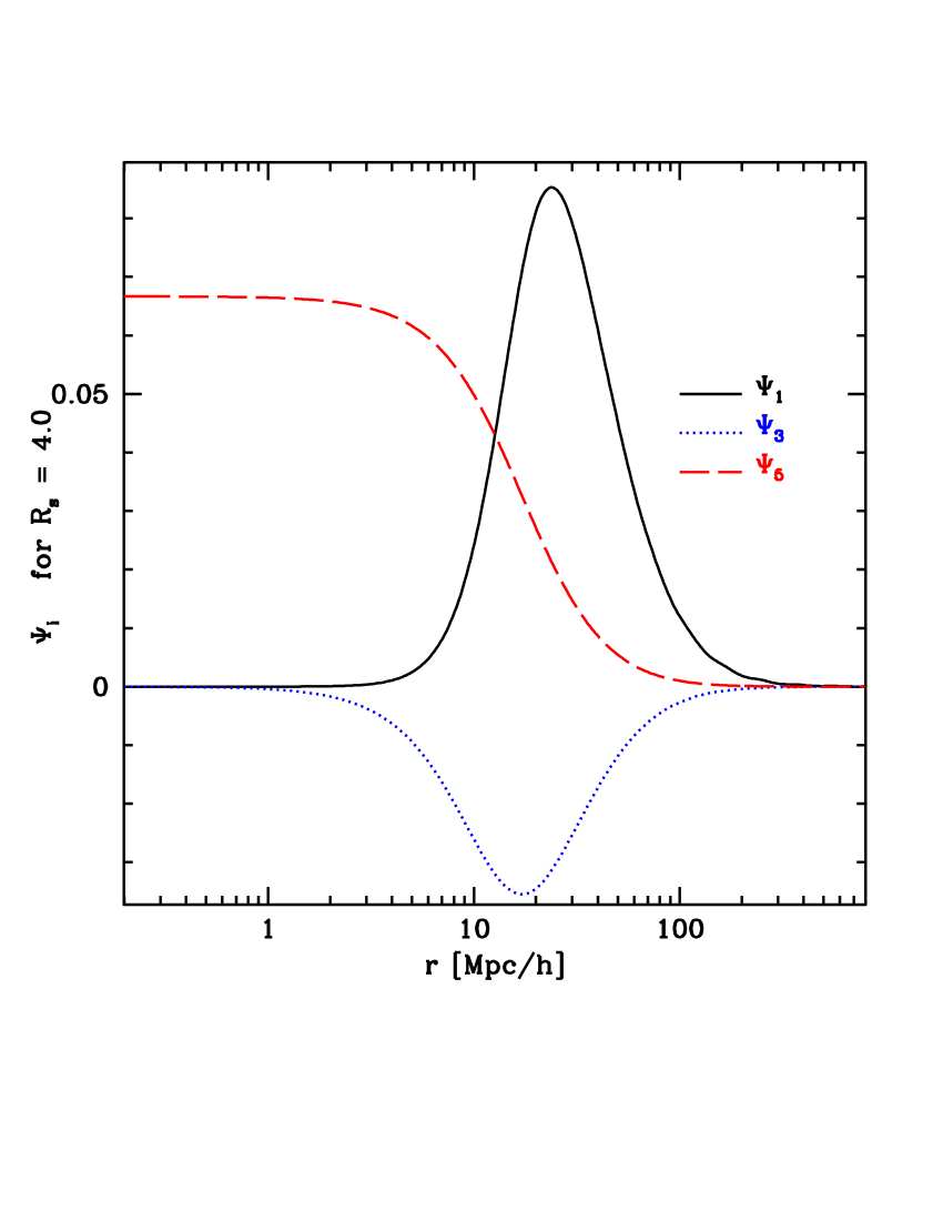
Figure 8: The three kernel functions $\Psi_{1},\Psi_{3},\Psi_{5}$ (Eq. 23) used to calculate the mean shear properties, for a Gaussian window function with smoothing $R_{s}=4h^{-1}Mpc$. The natural scale is about 10-20 $h^{-1}Mpc$ comoving, larger than the $R_{s}$ in part due to the softness of the cutoff in the window function.

For $\Psi^{Z}_{i}$’s correlations, the associated basis functions are (e.g., White (2014)):

$$\begin{array}[]{lll}\Psi_{2}(r)&=&\frac{1}{\sigma^{2}}\int_{0}^{\infty}d\ln k\Delta_{\delta}^{2}(k)\frac{W_{R}(k)^{2}}{k}(-\frac{1}{5}j_{1}(kr)-\frac{1}{5}j_{3}(kr))\\ \Psi_{4}(r)&=&\frac{1}{\sigma^{2}}\int_{0}^{\infty}d\ln k\Delta_{\delta}^{2}(k)\frac{W_{R}(k)^{2}}{k}j_{3}(kr)\;.\\ \end{array}$$ (24)

These are used to calculate the mean displaced edges of the cosmological structures shown as solid black lines in Fig. 3.

Appendix B Subtleties in fixing $\bar{\lambda}_{i}=\bar{\lambda}_{i,CA}$

Method 1 of assigning $\lambda^{0}_{i}$ (in §3.1) constrains its value implicitly by requiring the average shear in a mean object of a certain kind, centered at the origin, to be equal to the mean value of shear for that kind of object in Eq. 11. In addition to not always being able to solve this constraint by systematic trial and error, there are also conceptual subtleties with this approach, although there is an intuitive appeal to requiring the average of the shear within the central mean object in our construction to be the analytically calculated average of the shear within that type of object, $\bar{\lambda}_{i,CA}$. One complication was already noted for voids, as constructing a mean void volume is challenging when there is no boundary between a mean “void” configuration and the mean background, i.e. no mean void “size”. In practice, restricting to halos, filaments and sheets, we took objects centered on each kind of structure and calculated the average shear within these objects for a given $\lambda_{\rm th}$. We then varied the central shear until the mean shear within each object was the one given by Eq. 11 for that object.

However, the mean maps often have more than just the central type of object and the void structure in them; all four structures can be present in a mean map centered on any one type of structure. So when one calculates the mean shear in the mean objects of a certain structure, one possible way is to include the contributions from all the different maps where that structure appears. That is all regions with that given structure, even if not part of the central object, should be included as well. If the average in the mean maps is chosen to include the contributions from these other regions, the calculation of mean shear becomes more complicated.

We give an example by showing how adding these regions to calculate the mean shear can affect the calculation of mean shear for filaments. Generally, a mean halo at the origin also has filament regions around it. So in addition to the mean filament region around the origin, when the origin is a filament, the mean of filament shears including other regions would include the shear contribution from filament regions around the mean central halo, calculated for the same threshold. The relative contributions of these filaments in the different maps, filaments around mean halos, around central mean filaments, (and sheets and voids in some cases), can be estimated if one breaks down the volume fraction for each kind of object into contributions from each configuration: i.e. filaments when there is a mean halo at center, when there is a mean filament at center and when there is a mean sheet at center. This is

$$\begin{array}[]{ll}V_{\rm tot}f_{Vf}=&N_{\rm halo}\bar{V}_{\rm fil\in halo}+N_{\rm fil}\bar{V}_{\rm fil}+N_{\rm sheet}\bar{V}_{\rm fil\in sheet}\\ &+N_{\rm voids}\bar{V}_{\rm fil\in voids}\;.\end{array}$$ (25)

Here the volume fractions $f_{Vh},f_{Vf},f_{Vs},f_{Vv}$ of each structure are available from Eq. 11, and $\bar{V}_{\rm fil\in halo}$ is the filament volume associated with each mean halo, etc., found by constructing the mean halo, etc. and measuring the volume. These volumes depends upon the central shears which one is trying to find. This is especially challenging if contributions to the mean filamentary shear are large from any mean map besides that centered on the mean filament, and gets even more self-referential once filaments appear in the outskirts of sheets or halos appear in the outskirts of filaments, i.e. the last two terms $\bar{V}_{\rm fil\in sheet},\bar{V}_{\rm fil\in voids}\neq 0$.

For some $\lambda_{\rm th}$ these additional terms $N_{\rm halo}\bar{V}_{\rm fil\in halo}+N_{\rm sheet}\bar{V}_{\rm fil\in sheet}+N_{\rm voids}\bar{V}_{\rm fil\in voids}$ seem small. Then the calculation ignoring these other terms, that is, averaging the filament shear only over the mean object centered on the origin which is a filament, seems justified even in this more complicated interpretation (and similarly for sheets and halos in their respective cases). For filaments these other terms can be estimated for size by the following method. For $\lambda_{\rm th}$ large enough, the mean halo structure only appears when it is the central object, so $\lambda^{0}_{i}$ can be found for the mean halo by imposing $\lambda^{0}_{i}=\bar{\lambda}_{i,CA}$ for a mean halo centered at the origin. Also, again for $\lambda_{\rm th}$ large enough, $\bar{V}_{\rm fil\in sheet}=\bar{V}_{\rm fil\in voids}=0$. Then filaments only appear around the central mean halo and as the central mean filament. So we have:

$$\begin{array}[]{ll}V_{\rm tot}f_{Vh}&=N_{\rm halo}\bar{V}_{\rm halo}\\ V_{\rm tot}f_{Vf}&=N_{\rm halo}\bar{V}_{\rm fil\in halo}+N_{\rm fil}\bar{V}_{\rm fil}\;.\end{array}$$ (26)

and the filamentary volume around the mean halo, $\bar{V}_{\rm fil\in halo}$ is determined by the mean halo, already in hand. As we also know $f_{Vh}/f_{Vf}$, we can constrain

$$\frac{N_{\rm halo}V_{\rm fil\in halo}}{N_{\rm fil}V_{\rm fil}}=\frac{V_{\rm fil\in halo}}{\frac{f_{Vf}}{f_{Vh}}V_{\rm halo}-V_{\rm fil\in halo}}\;.$$ (27)

This can be used to see if the fraction of mean filament shear due to filaments around halos is large relative to that due to a filament centered at the origin. For $R_{s}=4h^{-1}Mpc$ halos and $\lambda_{\rm th}=0.762$, $V_{\rm fil\in halo}\sim 2V_{\rm halo}$ and $f_{Vf}/f_{Vh}=1/72$, giving a fraction of filament volume due to filaments around halos of about 1/35, which we thus neglected in calculating the filament central value shown in Fig. 2. Repeating the argument for sheets, for this threshold and smoothing, the relatively large sheet to filament volume fraction $f_{Vs}/f_{Vf}\sim 1/14$, combined with the large $\bar{V}_{\rm sheet\in fil}$, makes $\bar{V}_{\rm sheet\in fil}$ too large to reasonably neglect in this interpretation. In Fig. 2 we thus considered instead $\lambda_{\rm th}=1.25$ to impose $\bar{\lambda}_{i}=\bar{\lambda}_{i,CA}$ in a sheet configuration. (For the other scale studied in detail by Alonso, Eardley & Peacock (2014), $R_{s}=10h^{-1}Mpc$, filament contributions around halos and the filament to halo fraction (1/12) were both too large for their $\lambda_{\rm th}=0.261$ to permit neglect of $\bar{V}_{\rm fil\in halo}$.) One could include these subleading contributions directly instead of going to regimes where they can be neglected, as well, in some cases, when halos are not found in filament edges, and filaments are not found in sheet edges. It would be interesting to further explore this interpretation, although the issues with voids might make it difficult to push it very far.

This mean halo/filament/sheet interpretation and argument also gives a characteristic mean halo, filament and sheet volume and an expression for $N_{\rm fil}$ in terms of the number of halos, the volume fractions of filaments and halos and the mean volumes of filaments and halos. For the simplest case, for instance, $N_{\rm fil}=\frac{N_{\rm halo}}{V_{\rm fil}}(\frac{f_{Vf}}{f_{Vh}}V_{\rm halo}-V_{\rm fil\in halo})$, and analogously for sheets.

$M(R_{s})/h^{-1}M_{\odot}$	$R_{s}/h^{-1}Mpc$	$\lambda_{\rm th}$	V $\rho_{b}$ $h^{-1}M_{\odot}$	x, y, z max	$\langle\delta\rangle$	$\lambda^{0}_{i}$ $\bar{\lambda}_{i}$
halo 1.0e+14	4.2	0.54	4.70e+13	5.52 6.67 4.36	2.03	1.35, 0.93, 0.65 1.22 0.85 0.58
halo 5.0e+14	7.2	0.81	9.74e+13	5.93 7.00 5.65	1.79	1.63, 1.20, 0.92 1.53 1.14 0.86
halo 1.0e+15	9.0	0.98	1.03e+14	5.52 6.36 6.22	1.74	1.84, 1.39, 1.09 1.77 1.35 1.04
void 1.0e+14	4.2	0.00	1.20e+13	4.06 3.13 2.59	-2.88	-0.77, -1.30, -1.84 -0.74 -1.26 -1.77
void 5.0e+14	7.2	0.00	1.52e+13	3.97 3.36 2.98	-2.83	-1.36, -1.90, -2.42 -1.33 -1.87 -2.38
void 1.0e+15	9.0	0.00	1.69e+13	3.97 3.52 3.13	-2.82	-1.75, -2.28, -2.81 -1.72 -2.25 -2.77

Table 1: Properties for halos (top) and voids (bottom) for objects using the smoothing scales $R_{s}$ and thresholds $\lambda_{\rm th},\delta$ of Papai and Sheth (2013). These objects have both a $\lambda_{\rm th}$ and $\delta$ constraint at the origin. For halos, $\lambda_{\rm th}=0.41/\sigma(R_{s})$, $\delta>1.686/\sigma(R_{s})$. For voids, $\lambda_{\rm th}=0$, $\delta<-2.8/\sigma(R_{s})$. The mass of the mean halo volumes tends to be smaller than that associated with the smoothing scale.

Appendix C Stacked halos and voids with a different $\lambda^{0}_{i}$ constraint

This method for calculating mean shear was used by Papai and Sheth (2013) to find the mean shear due to a given configuration at the origin. They took the origin to correspond to 1) the sum of all halos with mass above some smoothing scale and 2) all voids associated with a smoothing scale, at large distances and final times. To find the central values of shear, they imposed conditions both on the eigenvalues of the shear individually and on their sum (the density). We give here properties of the mean configuration maps for their boundary conditions at the origin. Note that we consider the mean smoothed values given their boundary conditions (that is we smooth the shear both at the origin and at the position it is being measured).

They chose $\lambda^{0}_{i}=\bar{\lambda}_{i,RS}$, where the latter was found by integrating Eq. 11 with either their halo or void constraints but with an additional constraint in the measure, a step function in the density. For halos, $\lambda_{\rm th}(\sigma)=0.41/\sigma$ and $\sum_{i}\lambda_{i}>1.686/\sigma$, for voids, $\lambda_{\rm th}(\sigma)=0$ and $\sum_{i}\lambda_{i}<-2.8/\sigma$. This is analogous to our choice of central shear 2, except for the additional density constraint. In addition, voids and halos have different thresholds $\lambda_{\rm th}$.

For the comparison with simulations, as $R_{s}$ increases, $\sigma(R_{s})$ decreases and $\lambda_{\rm th}$ increases, so halos with a larger smoothing (higher mass) will also obey the constraints for a lower $R_{s}$ (this was used in this note in §4). Thus for halos, Papai and Sheth (2013) interpret the resulting shear at the origin $\lambda^{0}_{i}$ as due to the sum of halos with mass associated with $R_{s}$ and above. They take simulated halos with masses corresponding to $R_{s}$ and above in a numerical simulation, stack them, and compare measured and analytically predicted anisotropies in density at large distances, finding reasonable agreement.

They consider masses $10^{14},5\times 10^{14},10^{15}h^{-1}M_{\odot}$, from which we find $R_{s}$. In Table 1, we show halo and void configurations they used, with the corresponding $R_{s},\lambda_{\rm th}$, volume ($\sim M$), shape, average $z=0$ (Eulerian) overdensity, and $\lambda^{0}_{i}$, $\bar{\lambda}_{i}$. We use a Gaussian window function.

Interestingly, for these constraints, the central value of shear and the average value in the halo or void volume are very close. The density cut is a stringent constraint on the shear and the average density in the regions is close to the minimum (maximum for voids) imposed density. The associated volumes for the halos correspond to smaller masses than the Lagrangian volumes of the halos associated with $R_{s}$.

References

- Alonso, Eardley & Peacock (2014) Alonso, D., Eardley, E., Peacock, J.A., 2014, arXiv:1406.4159
- Bardeen, Bond, Kaiser & Szalay (1986) Bardeen, J.M., Bond, J.R., Kaiser, N., Szalay, A.S., 1986, ApJ, 304, 15
- Blumenthal, Faber, Primack & Rees (1984) Blumenthal, G. R., Faber, S. M., Primack, J. R., Rees, M. J., 1984, Nature, 311, 517
- Bond, Kofman & Pogosyan (1996) Bond J. R., Kofman L., Pogosyan D., 1996, Nature, 380, 603
- Borzyszkowski, Ludlow & Porciani (2014) Borzyszkowski, M., Ludlow, A.D., Porciani, C., 2014, MNRAS, 445, 4124
- Colberg (2007) Colberg, J. M., 2007, MNRAS, 375, 337
- Dalal, White, Bond & Shirokov (2008) Dalal, N., White, M., Bond, J.R., Shirokov, A., 2008, ApJ, 687, 12
- Desjacques (2008) Desjacques, V., 2008, MNRAS, 388, 638
- Desjacques and Smith (2008) Desjacques, V., Smith, R.E., 2008, PRD78, 023527
- Despali, Tormen & Sheth (2013) Despali, G., Tormen, G., Sheth, R.K., 2013, MNRAS, 431, 1143
- Doroshkevich (1970) Doroshkevich, A.G., 1970, Astrophysics, 6, 320
- Einasto et al. (1984) Einasto, J., Klypin, A.A., Saar, E., Shandarin, S.F., 1984, MNRAS, 206, 529
- Eisenstein & Hu (1999) Eisenstein, D., Hu, W., 1999, ApJ, 511, 5
- Elia, Ludlow & Porciani (2012) Elia, A., Ludlow, A.D., Porciani, C., 2012, MNRAS, 421, 3472
- Forero-Romero et al (2009) Forero-Romero, J.E., Hoffman, Y., Gottlober, S., Klypin, A., Yepes, G., 2009, MNRAS, 396, 1815
- Hahn et al (2007) Hahn, O., Porciani, C., Carollo, C. M., Dekel, A., 2007, MNRAS, 375, 489
- Hoffman et al (2012) Hoffman, Y., Metuki, O., Yepes, G., Gottlober, S., Forero-Romero, J.E., Libeskind, N.I., Knebe, A., 2012, MNRAS, 425, 2049
- Jasche, Leclercq & Wandelt (2015) Jasche, J., Leclercq, F., Wandelt, B.D., 2015, JCAP, 1, 36
- Kaiser (1984) Kaiser, N., 1984, ApJL, 284, 9
- Lam, Sheth & Desjacques (2009) Lam, T.Y., Sheth, R.K., Desjacques, V., 2009, MNRAS, 399, 1482
- Leclercq, Jasche & Wandelt (2015a) Leclercq, F., Jasche, J., Wandelt, B., 2015a, JCAP, 6, 15
- Leclercq, Jasche & Wandelt (2015b) Leclercq, F., Jasche, J., Wandelt, B., 2015b, JCAP, 5, 26
- Leclercq, Jasche & Wandelt (2015c) Leclercq, F., Jasche, J., Wandelt, B., 2015c, A&A Letters, 576, 17
- Lee and Shandarin (1998) Lee, J., Shadarin, S.F., 1998, ApJ, 500, 14
- Ludlow, Borzyszkowski & Porciani (2014) Ludlow, A.D., Borzyszkowski,M., Porciani, C., 2014, MNRAS, 445, 4110
- Ludlow and Porciani (2011) Ludlow, A.D., Porciani, C., 2011, MNRAS,413,1961
- Mo, van den Bosch & White (2010) Mo, H., van den Bosch, F., White, S.D.M., 2010, “Galaxy Formation and Evolution”, Cambridge University Press, Cambridge
- Papai and Sheth (2013) Papai, P., Sheth, R.K., 2013, MNRAS, 429, 1133
- Peacock (1998) Peacock, J. A., 1998, “Cosmological Physics”, Cambridge University Press, Cambridge
- Pillepich, Porciani & Hahn (2010) Pillepich, A., Porciani, C., Hahn, O., 2010, MNRAS, 402, 191
- Planck Collaboration (2013) Planck Collaboration, 2013, A& A, 571, 16
- Press & Schechter (1974) Press, W.H., Schechter, P., 1974, ApJ, 187, 425
- Pogosyan et al (2009) Pogosyan, D., Pichon, C., Gay, C., Prunet, S., Cardoso, J.F., Sousbie, T., Colombi, S., 2009, MNRAS, 396, 635
- Robertson, et al (2009) Robertson, B.E., Kravtsov, A.V., Tinker, J., Zentner, A.R., 2009, ApJ 696, 636
- Robles, Dominguez-Tenreiro, Onorbe & Martinez-Serrano (2015) Robles, S., Dominguez-Tenreiro, R., Onorbe, J., Martinez-Serrano, F.J., 2015, arXiv: 1504.06297
- Shandarin & Zel’dovich (1983) Shandarin, S.F., Zel’dovich, Ia. B., 1983, Comments on Astrophysics, 10, 33
- Shandarin (2009) Shandarin, S., 2009, JCAP, 02, 031
- Shen, Abel, Mo & Sheth (2006) Shen, J., Abel, T., Mo, H.J., Sheth, R.K., 2006, ApJ, 645, 783
- Tallinn conference (2014) “Proceedings of IAUS 308: The Zel’dovich Universe: Genesis and Growth of the Cosmic Web”, to appear.
- Tinker et al (2008) Tinker, J., Kravtsov, A.V., Klypin, A., Abazajian, K., Warren, M., Yepes, G., Gottlober, S., Holz, D.E., 2008, ApJ, 688, 709
- White (2001) White M., 2001, A&A, 367, 27
- White (2014) White, M., 2014, MNRAS, 439, 3630
- Zel’dovich, Einasto & Shandarin (1982) Zel’dovich, Ia.B., Einasto, J., Shandarin, S.F., 1982, Nature, 300, 407