New Geometric Algorithms
for Fully Connected Staged Self-Assembly

Abstract

We consider staged self-assembly systems, in which square-shaped tiles can be added to bins in several stages. Within these bins, the tiles may connect to each other, depending on the glue types of their edges. Previous work by Demaine et al. showed that a relatively small number of tile types suffices to produce arbitrary shapes in this model. However, these constructions were only based on a spanning tree of the geometric shape, so they did not produce full connectivity of the underlying grid graph in the case of shapes with holes; self-assembly of fully connected assemblies with a polylogarithmic number of stages was left as a major open problem. We resolve this challenge by presenting new systems for staged assembly that produce fully connected polyominoes in $\mathcal{O}(\log^{2}n)$ stages, for various scale factors and temperature $\tau=2$ as well as $\tau=1$. Our constructions work even for shapes with holes and use only a constant number of glues and tiles. Moreover, the underlying approach is more geometric in nature, implying that it promises to be more feasible for shapes with compact geometric description.

1 Introduction

In self-assembly, a set of simple tiles form complex structures without any active or deliberate handling of individual components. Instead, the overall construction is governed by a simple set of rules, which describe how mixing the tiles leads to bonding between them and eventually a geometric shape.

The classic theoretical model for self-assembly is the abstract tile-assembly model (aTAM). It was first introduced by Winfree [15, 13]. The tiles used in this model are building blocks, which are unrotatable squares with a specific glue on each side. Equal glues have a connection strength and may stick together. The glue complexity of a tile set $T$ is the number of different glues on all the tiles in $T$, while the tile complexity of $T$ is the number of different tile types in $T$. If an additional tile wants to attach to the existing assembly by making use of matching glues, the sum of corresponding glue strengths needs to be at least some minimum value $\tau$, which is called the temperature.

A generalization of the aTAM called the two-handed assembly model (2HAM) was introduced by Demaine et al. [4]. While in the aTAM, only individual tiles can be attached to an existing intermediate assembly, the 2HAM allows attaching other partial assemblies. If two partial assemblies (“supertiles”) want to assemble, then the sum of the glue strength along the whole common boundary needs to be at least $\tau$.

In this paper we consider the staged tile assembly model introduced in [4], which is based on the 2HAM. In this model the assembly process is split into sequential stages that are kept in separate bins, with supertiles from earlier stages mixed together consecutively to gain new supertiles. We can either add a new tile to an existing bin, or we pour one bin into another bin, such that the content of both gets mixed; afterwards, unassembled parts get removed. The overall number of stages and bins of a system are the stage complexity and the bin complexity. Demaine et al. [4] achieved several results summarized in Table 1. Most notably, they presented a system (based on a spanning tree) that can produce arbitrary polyomino shapes $P$ in $\mathcal{O}(\mbox{\em diameter})$ many stages, $\mathcal{O}(\log N)=\mathcal{O}(\log n)$ bins and a constant number of glues, where $N$ is the number of unit squares, called pixels, whose union forms $P$, $n$ is the size of the bounding box, i.e., a smallest square containing $P$, and the diameter is measured by the maximum length of a shortest path between any two pixels in the adjacency graph of the pixels in $P$; this can be as big as $N$. The downside is that the resulting supertiles are not fully connected. For achieving full connectivity, only the special case of monotone shapes was resolved by a system with $\mathcal{O}(\log n)$ stages; for hole-free shapes, Demaine et al. [4] were able to give a system with full connectivity, scale factor 2, but $\mathcal{O}(n)$ stages. This left a major open problem: designing a staged assembly system with full connectivity, polylogarithmic stage complexity and constant scale factor for general shapes.

Our results. We show that for any polyomino, even with holes, there is a staged assembly system with the following properties, both for $\tau=2$ and $\tau=1$.

1. polylogarithmic stage complexity,

2. constant glue and tile complexity,

3. constant scale factor,

4. full connectivity.

See Table 1 for an overview. The main novelty of our method is to focus on the underlying geometry of a constructed shape $P$, instead of just its connectivity graph. This results in bin complexities that are a function of $k$, the number of vertices of $P$: while $k$ can be as big as $\Theta(n^{2})$, $n$ can be arbitrarily large for fixed $k$, implying that our approach promises to be more suitable for constructing natural shapes with a clear geometric structure.

Lines and Squares	Glues	Tiles	Bins	Stages	$\tau$	Scale	Conn.	Planar
Line [4]	3	6	7	$\mathcal{O}(\log n)$	1	1	full	yes
Square — Jigsaw techn. [4]	9	$\mathcal{O}(1)$	$\mathcal{O}(1)$	$\mathcal{O}(\log n)$	1	1	full	yes
Square — $\tau=2$ (Sect. 3.1)	4	$\mathcal{O}(1)$	$\mathcal{O}(1)$	$\mathcal{O}(\log n)$	2	1	full	yes
Arbitrary Shapes	Glues	Tiles	Bins	Stages	$\tau$	Scale	Conn.	Planar
Spanning Tree Method [4]	2	16	$\mathcal{O}(\log n)$	$\mathcal{O}(diameter)$	1	1	partial	no
Monotone Shapes [4]	9	$\mathcal{O}(1)$	$\mathcal{O}(n)$	$\mathcal{O}(\log n)$	1	1	full	yes
Hole-Free Shapes [4]	8	$\mathcal{O}(1)$	$\mathcal{O}(N)$	$\mathcal{O}(N)$	1	2	full	no
Shape with holes (Sect. 3.2)	$\color[rgb]{0,0,0}6\color[rgb]{0,0,0}$	$\mathcal{O}(1)$	$\mathcal{O}(k)$	$\mathcal{O}(\log^{2}n)$	2	3	full	no
Hole-Free Shapes (Sect. 3.2)	$\color[rgb]{0,0,0}6\color[rgb]{0,0,0}$	$\mathcal{O}(1)$	$\mathcal{O}(k)$	$\mathcal{O}(\log n)$	2	3	full	no
Hole-Free Shapes (Sect. 4.1)	$18$	$\mathcal{O}(1)$	$\mathcal{O}(k)$	$\mathcal{O}(\log^{2}n)$	1	4	full	no
Shape with holes (Sect. 4.2)	$20$	$\mathcal{O}(1)$	$\mathcal{O}(k)$	$\mathcal{O}(\log^{2}n)$	1	6	full	no

Table 1: Overview of results from [4] and this paper. The number of pixels of $P$ is denoted by $N\in\mathcal{O}(n^{2})$, $n$ is the side length of a smallest bounding square, while $k$ is the number of vertices of the polyomino, with $k\in\Omega(1)$ and $k\in\mathcal{O}(N)$. The diameter is the maximum of all shortest paths between any two pixels in the adjacency graph of the corresponding shape.

Related work. As mentioned above, our work is based on the 2HAM. There is a variety of other models, e.g., see [2]. A variation of the staged 2HAM is the Staged Replication Assembly Model by Abel et al. [1], which aims at reproducing supertiles by using enzyme self assembly.  Another variant is the Signal-passing Tile Assembly Model introduced by Padilla et al. [10].

Other related geometric work by Cannon et al. [3] and Demaine et al. [5] considers reductions between different systems, often based on geometric properties. Fu et al. [8] use geometric tiles in a generalized tile assembly model to assemble shapes. Fekete et al. [7] study the power of using more complicated polyominoes as tiles.

Using stages has also received attention in DNA self assembly. Reif [12] uses a stepwise model for parallel computing. Park et al. [11] consider assembly techniques with hierarchies to assemble DNA lattices. Somei et al. [14] use a stepwise assembly of DNA tiles. Padilla et al. [9] include active signaling and glue activation in the aTAM to control hierarchical assembly of Robinson patterns. None of these works considers complexity aspects.

2 The Staged Assembly Model

In this section, we present basic definitions common to most assembly models, followed by a description of the staged assembly model, and finally we define various metrics to measure the efficiency of a staged assembly system. Staged assembly systems were introduced by Demaine et al. [4]. As we use their basic definitions, we quote the corresponding framework (mostly verbatim) for self-containedness of this paper.

Polyominoes.

A polyomino $P$ is a polygon with axis-parallel edges of integer length. (See Figure 1.) A vertex of $P$ is a reflex vertex, if its interior angle is $3\pi/2$. Every polyomino can be decomposed into a set of unit squares, called pixels; without loss of generality, we assume they are centered at points from $\mathbb{Z}^{2}$; as described below, this means they correspond to tile positions in a configuration. The degree of a pixel is the number of (vertically or horizontally) adjacent pixels in the polyomino. A pixel is a boundary pixel if at least one of the eight (axis parallel or diagonal) neighbor positions is not occupied by a pixel in $P$. A boundary pixel $p$ is an ordinary boundary pixel if precisely two (say, $p^{\prime}$ and $p^{\prime\prime}$) of its four vertical or horizontal neighbor pixels in $P$ are boundary pixels, and the positions of $p$, $p^{\prime}$, $p^{\prime\prime}$ are collinear; a boundary pixel is a corner pixel of $P$ if is not an ordinary boundary pixel. The corner set of a polyomino is the set of all corner pixels along all boundaries.

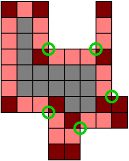
Figure 1: A polyomino, its reflex vertices (indicated by green circles), its corner pixels (dark red) and its ordinary boundary pixels (light red).

Tiles and tile systems.

A (Wang) tile $t$ is a non-rotatable unit square defined by the ordered quadruple $\langle\mathop{\rm north}\nolimits(t),\mathop{\rm east}\nolimits(t),\mathop{\rm south}\nolimits(t),\mathop{\rm west}\nolimits(t)\rangle$ of glues on the four edges, also called sides, of the tile. Each glue is taken from a finite alphabet $\Sigma$, which includes a special “null” glue denoted null. For simplicity of bounds, we do not count the ${\rm null}$ glue in the glue complexity $g=|\Sigma|-1$.

A tile system is an ordered triple $\langle T,G,\tau\rangle$ consisting of the tileset $T$ (a set of distinct tiles), the glue function $G:\Sigma^{2}\rightarrow\{0,1,\dots,\tau\}$, and the temperature $\tau$ (a positive integer). It is assumed that $G(x,y)=G(y,x)$ for all $x,y\in\Sigma$ and that $G({\rm null},x)=0$ for all $x\in\Sigma$. Indeed, in all of our constructions $G(x,y)=0$ for all $x\neq y$, and each $G(x,x)\in\{1,2,\dots,\tau\}$. The tile complexity of the system is $|T|$.

Configurations.

A configuration, which we also call an assembly, is a function $C:\mathbb{Z}^{2}\rightarrow T\cup\{{\rm empty}\}$, where ${\rm empty}$ is a special tile that has the ${\rm null}$ glue on each of its four edges. The shape of a configuration $C$ is the set of positions $(i,j)$ that do not map to the ${\rm empty}$ tile. The shape of a configuration can be disconnected, corresponding to several distinct supertiles.

Adjacency graph and supertiles.

Define the adjacency graph $G_{C}$ of a configuration $C$ as follows. The vertices are coordinates $(i,j)$ such that $C(i,j)\neq{\rm empty}$. There is an edge between two vertices $(x_{1},y_{1})$ and $(x_{2},y_{2})$ if and only if $|x_{1}-x_{2}|+|y_{1}-y_{2}|=1$. A set of vertices $\{(x_{1},y_{1}),...,(x_{k},y_{k})\}$ are collinear if $x_{1}=\dots x_{k}$ or $y_{1}=\dots=y_{k}$. A vertex of a configuration $C$ is a vertex $(i,j)$ of $G_{C}$ if there are $x,y\in\{-1,1\}$ such that $C(i+x,j),C(i,j+y)={\rm empty}$ and $C(i-x,j),C(i,j-y)\neq{\rm empty}$. A vertex $C(i,j)$ of $C$ is reflex if $C(i,j)$ is adjacent to one position that is the empty tile.

A supertile is a maximal connected subset $G^{\prime}$ of $G_{C}$, i.e., $G^{\prime}\subseteq G_{C}$ such that, for every connected subset $H$, if $G^{\prime}\subseteq H\subseteq G_{C}$, then $H=G^{\prime}$. For a supertile $S$, let $|S|$ denote the number of nonempty positions (tiles) in the supertile. We call $|S|$ the size of $S$. Throughout this paper, we informally refer to (lone) tiles as a special case of supertiles.

If every two adjacent tiles in a supertile share a positive strength glue type on abutting edges, the supertile is fully connected. All provided assembly systems in this paper are fully connected.

Staged assembly systems.

For any two supertiles $X$ and $Y$, the combination set $C^{\tau}_{(X,Y)}$ of $X$ and $Y$ is defined to be the set of all supertiles obtainable by placing $X$ and $Y$ adjacent to each other (without overlapping) such that, if we list each newly coincident edge $e_{i}$ with edge strength $s_{i}$, then $\sum s_{i}\geq\tau$.

A bin is a pair $(S,\tau)$, where $S$ is a set of initial supertiles whose tile types are contained in a given set of tile types $T$, and $\tau$ is a temperature parameter. For a bin $(S,\tau)$, the set of produced supertiles $P^{\prime}_{(S,\tau)}$ is defined recursively as follows: (1) $S\subseteq P^{\prime}_{(S,\tau)}$ and (2) for any $X,Y\in P^{\prime}_{(S,\tau)}$, $C^{\tau}_{(X,Y)}\subseteq P^{\prime}_{(S,\tau)}$. The set of terminally produced supertiles of a bin $(S,\tau)$ is $P_{(S,\tau)}=\{X\in P^{\prime}\mid Y\in P^{\prime}$, $C^{\tau}_{(X,Y)}=\emptyset\}$. The set of supertiles $P$ is uniquely produced by bin $(S,\tau)$ if each supertile in $P^{\prime}$ is of finite size.

We can create a bin of a single tile type $t\in T$, we can merge multiple bins together into a single bin, and we can split the contents of a given bin into multiple new bins. In particular, when splitting the contents of a bin, we assume the ability to extract only the unique terminally produced set of supertiles $P$, while filtering out additional partial assemblies in $P^{\prime}$.

An $r$-stage $b$-bin mix graph $M$ consists of $rb+1$ vertices, $m_{*}$ and $m_{i,j}$ for $1\leq i\leq r$ and $1\leq j\leq b$, and an arbitrary collection of edges of the form $(m_{r,j},m_{*})$ or $(m_{i,j},m_{i+1,k})$ for some $i,j,k$.

A staged assembly system is a $3$-tuple $\langle M_{r,b},\{T_{i,j}\},\{\tau_{i,j}\}\rangle$, where $M_{r,b}$ is an $r$-stage $b$-bin mix graph, each $T_{i,j}$ is a set of tile types, and each $\tau_{i,j}$ is an integer temperature parameter. Given a staged assembly system, for each $1\leq i\leq r$, $1\leq j\leq b$, we define a corresponding bin $(R_{i,j},\tau_{i,j})$, where $R_{i,j}$ is defined as follows:

1. $R_{1,j}=T_{1,j}$ (this is a bin in the first stage);

2. For $i\geq 2$, $\displaystyle R_{i,j}=\Big{(}\bigcup_{k:\ (m_{i-1,k},m_{i,j})\in M_{r,b}}P_{(R_{(i-1,k)},\tau_{i-1,k})}\Big{)}\cup T_{i,j}$.

3. $\displaystyle R_{*}=\bigcup_{k:\ (m_{r,k},m_{*})\in M_{r,b}}P_{(R_{(r,k)},\tau_{r,k)})}$.

The set of terminally produced supertiles for a staged assembly system are defined as $P_{(R_{*},\tau_{*})}$. A staged assembly system uniquely produces the set of supertiles $P_{(R_{*},\tau_{*})}$ if in each bin the terminal supertiles are unique.

Throughout this paper, we assume that, for all $i,j$, $\tau_{i,j}=\tau$ for some fixed global temperature $\tau$, and we denote a staged assembly system as $\langle M_{r,b},\{T_{i,j}\},\tau\rangle$.

The following metrics are considered: The tile complexity $|\bigcup T_{i,j}|$, the bin complexity $b$, the stage complexity $r$, and the temperature $\tau$.

A staged assembly system is planar if supertiles have obstacle-free paths to reach their mates in every possible sequence of attachments. In a fully connected supertile, every two adjacent tiles have the same positive-strength glue along their common edge. Otherwise the supertile is partially connected.

3 Fully Connected Constructions for $\tau=2$

In the following, we consider fully connected assemblies for temperature $\tau=2$. We start by an approach for squares (Section 3.1). In Section 3.2 we describe how to extend this basic idea to assembling general polyominoes.

3.1 $n\times n$ Squares, $\tau=2$

For $\tau=2$ assembly systems, it is possible to develop more efficient ways for constructing a square. The construction is based on an idea by Rothemund and Winfree [13], which we adapt to staged assembly. Basically, it consists of connecting two strips by a corner tile, before filling up this frame; see Figure 2.

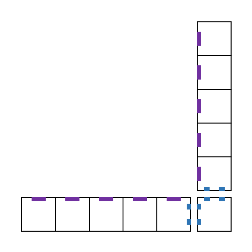
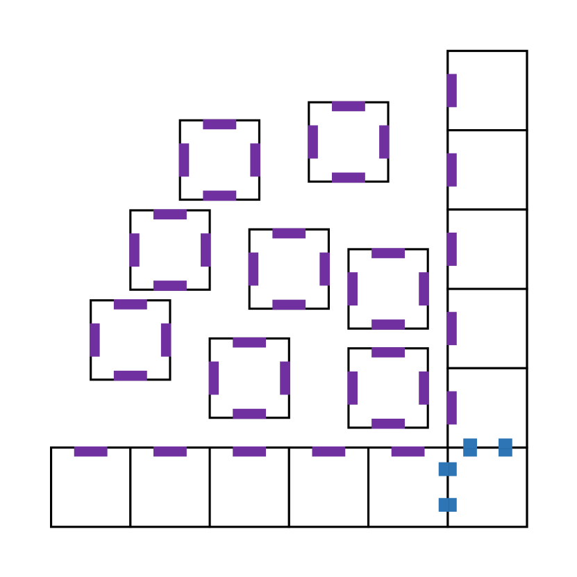
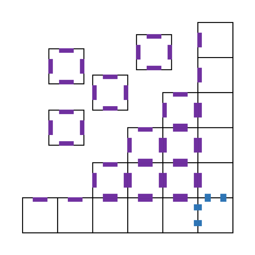
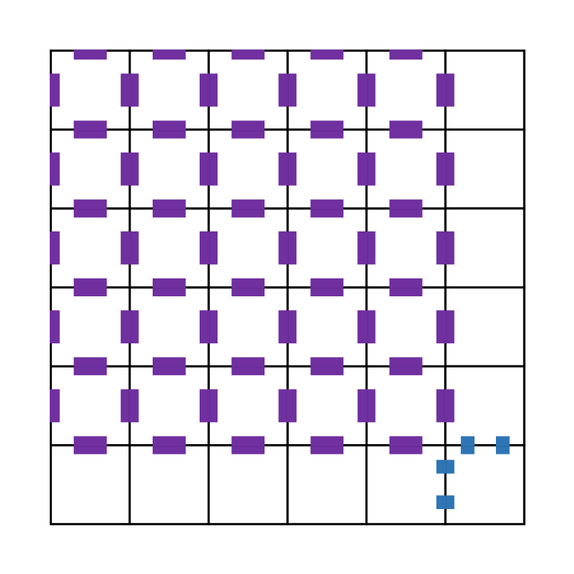
Figure 2: Construction of fully connected square using $\tau=2$ and a frame.

Theorem 3.1.

There exists a $\tau=2$ staged assembly system that assembles a fully connected $n\times n$ square with $\mathcal{O}(\log n)$ stages, $4$ glues, $14$ tiles and $7$ bins.

Proof.

The construction is an easy result of combining a known construction for lines by staged assembly with filling in squares in the aTAM with temperature $\tau=2$, as follows. First we construct the $1\times(n-1)$ strips with strength-2 glues. We know from [4] that a strip can be constructed in $\mathcal{O}(\log n)$ stages, three glues, six tiles and seven bins. Because both strips are perpendicular, they do not connect. Therefore, we can use all seven bins to construct both strips in parallel. For each strip we use tiles such that the edge toward the interior of the square has a strength-1 glue. In the next stage we mix the single corner tile with the two strips. Finally, we add a tile type with strength-1 glues on all sides. When the square is filled, no further tile can still connect, as $\tau=2$.

Overall, we need $\mathcal{O}(\log n)$ stages with four glues (three for the construction, one for filling up the square), 14 tiles (six for each of the two strips, one for the corner tile, one for filling up the square) and seven bins for the parallel construction of the two strips. ∎

3.2 Polyominoes with or without Holes, $\tau=2$

Our method for assembling a polyomino $P$ at $\tau=2$ generalizes the approach for building a square that is described in Section 3.1. The key idea is to scale $P$ by a factor of 3, yielding $P^{3}$; for this we first build a frame called the backbone, which is a specific spanning tree based on the union of all boundaries of $P^{3}$. This backbone is then filled up in a final stage by applying a more complex version of the flooding approach of Theorem 3.1. In particular, there is not only one flooding tile, but a constant set $S$ of such distinct tiles.

3.2.1 Definition and construction of the backbone.

In the following, we consider a scaled copy $P^{3}$ of a polyomino $P$, constructed by replacing each pixel by a $3\times 3$ square of pixels. We define the backbone of $P^{3}$ as follows; see Figure 3 for an illustration.

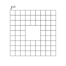
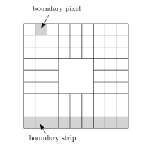
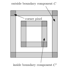
(a) 3-scaled polyomino $P^{3}$.	(b) Boundary pixels and strips.	(c) Outside and inside
		boundary components.
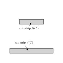
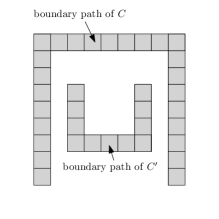
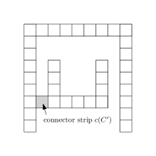
(d) Cut strip of $C$ and $C^{\prime}$.	(e) Boundary paths.	(f) Connector strip $c(C^{\prime})$.

Figure 3: Stepwise construction of the backbone of a 3-scaled polyomino $P^{3}$.

Definition 3.2.

A pixel of $P^{3}$ is a boundary pixel of $P^{3}$, if one of the pixels in its eight (axis-parallel or diagonal) neighbor pixels does not belong to $P^{3}$. A boundary strip of $P^{3}$ is a maximal set of boundary pixels that forms a contiguous (vertical or horizontal) strip, see Figure 3(b). A boundary component $C$ is a maximal connected component of boundary pixels.

Because of the scaling, an inside boundary component corresponds to precisely one inside boundary of $P^{3}$ (delimiting a hole), while the outside boundary component corresponds to the exterior boundary of $P^{3}$, see Figure 3(c). Furthermore, each boundary component $C$ has a unique decomposition into boundary strips: a circular sequence of boundary strips that alternate between vertical and horizontal, with consecutive strips sharing a single (“corner”) pixels.

Definition 3.3.

For an inside boundary component $C^{\prime}$, its cut strip $\ell(C^{\prime})$ is the leftmost of its topmost strips; for the outside boundary component, its cut strip $\ell(C)$ is the leftmost of its bottommost strips, see Figure 3(d).

A boundary path of the outside boundary component $C$ consists of the union of all its strips, with the exception of $\ell(C)$; for an inside boundary component $C^{\prime}$, it consists of $C^{\prime}\setminus\ell(C^{\prime})$; see Figure 3(e). Furthermore, the connector strip $c(C^{\prime})$ for an inside boundary component $C^{\prime}$ is the contiguous horizontal set of pixels of $P^{3}$ extending to the left from the leftmost bottommost pixel of $C^{\prime}$ and ending with the first encountered other boundary pixel of $P^{3}$; see Figure 3(f). Note that no tile of the boundary path is part of the connector strip. Then the backbone of $P^{3}$ is the union of all boundary paths and the connector strips of inside boundary components.

By construction, the backbone has a canonical decomposition into boundary strips and connector strips; furthermore, a pixel in the backbone of $P^{3}$ has degree three if and only if this pixel is adjacent to a pixel of a connector strip. For $h$ holes, only $2h$ pixels in the backbone can have degree three.

Overall, this yields a hole-free shape that can be constructed efficiently.

Lemma 3.4.

Let $k$ be the number of vertices of a $3$-scaled polyomino $P^{3}$. The corresponding backbone can be assembled in $\mathcal{O}(\log^{2}n)$ stages with $3$ glues, $\mathcal{O}(1)$ tiles and $\mathcal{O}(k)$ bins.

Proof.

The main idea is to give a hierarchical tree decomposition of the backbone $T$ into subtrees, all the way down to single pixels. Assembling the backbone is then performed in a bottom-up fashion from the tree decomposition. To this end, subtrees in the decomposition are split into smaller pieces by the removal of appropriate pixels. An important invariant is that each subtree is separated from the rest of the backbone by at most two pixels; when assembling the backbone in a bottom-up fashion from the tree decomposition, this ensures that a constant number of glues at the separating pixels suffices for assembling the whole backbone.

For decomposing the backbone, we observe that it consists of two types of components: strips and corner pixels; see Figure 4(b). By construction of the backbone, the degree of corner pixels is two or three, corresponding to the number of adjacent strips.

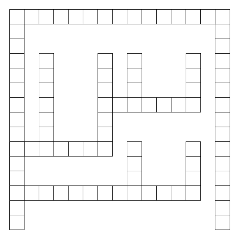
(a) A backbone of a scaled polyomino $P^{3}$.

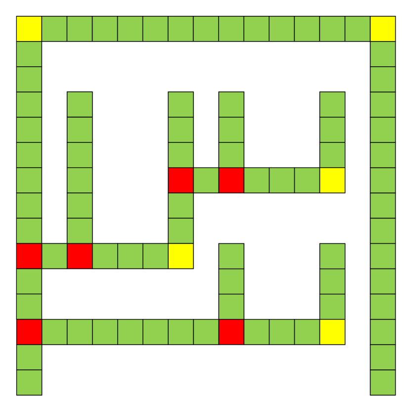
(b) A backbone decomposed into strips (green) and corner pixels of degree two (yellow) and degree three (red).

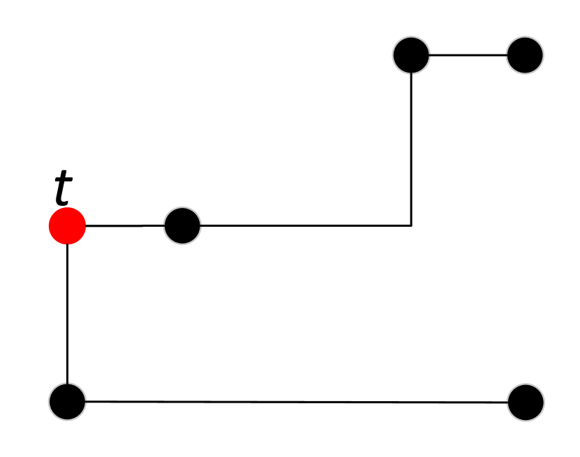
(c) Tree $T_{P}$ of degree-three pixels in the backbone. The red node is a tree median $t$ in $T_{P}$.

Figure 4: Example of a backbone, its decomposition by corner pixels, the corresponding tree $T_{P}$ of degree-3 pixels.

There are three levels of the decompostion, corresponding to splitting the tree by removal of (I) degree-three coner pixels (shown red in Figure 4(c)), (II) degree-two corner pixels (shown yellow in the figure) and (III) non-corner pixels (shown green in the figure). These splits are completely hierarchical: the level-I decomposition is carried out with respect to degree-three corner pixels until only pixels with degree two are left in all components, as shown in Figure 4; in level II, these components are further decomposed with respect to the corner pixels of degree two, such that only strips remain, i.e., subtrees without corner vertices that are shown green in Figure 4 (b). At the third and lowest level, the straight strips are decomposed until just individual pixels are left.

There are two key properties of the decomposition: (A) bounded tree depth, which ensures a small number of stages, and (B) bounded separation degree of subtrees, which ensures a small number of glues. The key ingredient for (A), a polylogarithmic recursion depth for all three decomposition levels, is that the splitting pixels are chosen such that the sizes of the split components are balanced. In particular, we ensure that the size of components is at most half of the size of the original component after at most two splits. This can be obtained by choosing among the pixels of the appropriate decomposition type one that is a (tree or path) median of a remaining backbone piece, i.e., a pixel whose removal leaves each connected component with at most half the number of vertices of the original tree. Performing this splitting operation recursively yields a recursion depth of at most $\mathcal{O}(\log k)$. In order to achieve (B), each subtree is separated from the rest of the backbone by the removal of at most two pixels from the rest of the backbone, special care is only necessary at level I, as subtrees in levels II and III do not have any vertices of degree higher than two; at level I, the property is achieved by a further subdivision into level I(a) (decomposition by removing a subtree median) and level I(b) (decomposition by removing a subpath median). Further details are described below.

Level I decomposition. Consider a tree $T_{P}$ whose vertices are the pixels of degree three in the backbone; two vertices are adjacent if their degree-three pixels can be connected by a path in the backbone that does not contain any other degree-three pixel (see Figure 4(c)). Because the backbone is hole-free, $T_{P}$ is a tree with maximum degree three. We decompose $T_{P}$ recursively as follows. Initially, we choose a vertex $t$ (see Figure 4(c)) that splits $T_{P}$ into connected components that each have at most half the number of nodes, i.e., a tree median resulting in subtrees of sizes at most $\lceil|T_{P}|/2\rceil$. The further decomposition of a nontrivial subtree $T^{\prime}_{P}$ of $T_{P}$ depends on its separation degree, which is the number of degree-three pixels that separate $T^{\prime}_{P}$ from the rest of $T_{P}$.

Level I(a) decomposition. If $T^{\prime}_{P}$ has separation degree one, i.e., it is separated from the rest of $T_{P}$ by a single degree-three vertex, we split $T^{\prime}_{P}$ into further pieces by removing a tree median of $T^{\prime}_{P}$; see Figure 5 (a). The resulting subtrees have separation degree one or two, and each piece has size at most $\lceil|T^{\prime}_{P}|/2\rceil$.

Level I(b) decomposition. If $T^{\prime}_{P}$ has separation degree two, it is separated from the rest of $T_{P}$ by two degree-three vertices, say, $v_{1}$ and $v_{2}$; see Figure 5 (b). If the path between $v_{1}$ and $v_{2}$ is a single edge in $T_{P}$, $T^{\prime}_{P}$ does not contain any further vertices, and we can proceed to level II. If there is a nontrivial path $W$ in $T^{\prime}_{P}$ between $v_{1}$ and $v_{2}$, we split $T^{\prime}_{P}$ by picking a path median of $W$. This results in three new subtrees; two of them (say, ${T^{\prime}_{P}}^{(1)}$ and ${T^{\prime}_{P}}^{(2)}$) have separation degree two, one (say, ${T^{\prime}_{P}}^{(3)}$) has separation degree 1. Clearly, ${T^{\prime}_{P}}^{(i)}\leq\lceil|T^{\prime}_{P}|/2\rceil$ for $i=1,2$. As ${T^{\prime}_{P}}^{(3)}$ has separation degree 1, its next decomposition will be level I(a), ensuring that its components will have size at most $\lceil|T^{\prime}_{P}|/2\rceil$ after this second split.

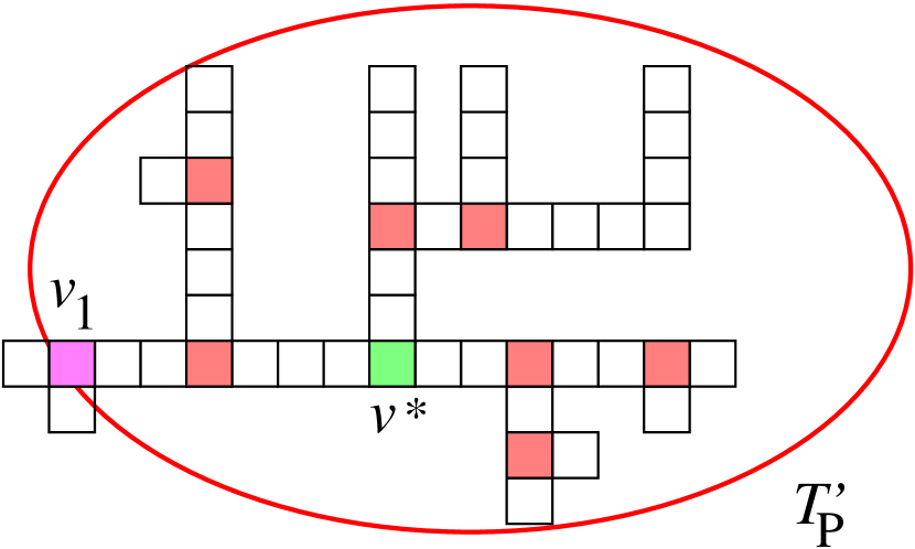
(a) Decomposition of level I(a): Subtree $T^{\prime}_{P}$ has one separation vertex ($v_{1}$, shown in purple). The next decomposition step is performed by splitting at the tree median, $v^{*}$.

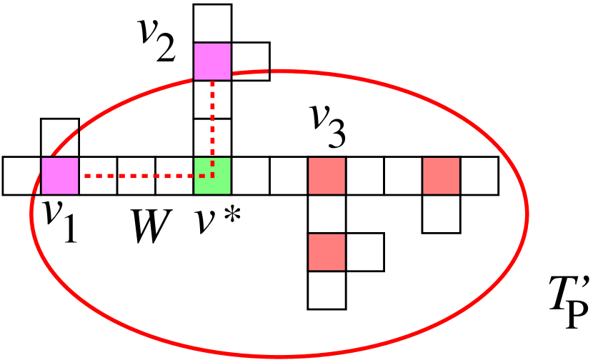
(b) Decomposition of level I(b): Subtree $T^{\prime}_{P}$ has two separation vertices ($v_{1}$ and $v_{2}$, shown in purple), connected by path $W$. The next decomposition step is performed by splitting at the path median, $v^{*}$, instead of the tree median $v_{3}$.

Figure 5: Decomposition step of level I.

By induction it follows that this recursion has a depth of $\mathcal{O}(\log|T_{P}|)=\mathcal{O}(\log k)\subseteq\mathcal{O}(\log n)$. Because each node has a degree of $3$, it follows that the width of the recursion tree is $\mathcal{O}(k)$, so a bin complexity of $\mathcal{O}(k)$ is guaranteed for assembling all level-I components.

Assembling the subtrees of the level-I decomposition can be ensured with just three glue types, as follows; see Figure 6. A degree-3 pixel $p$ is adjacent to three level-I components, say, $T_{1}$, $T_{2}$, $T_{3}$; at most two of them ($T_{1}$ and $T_{2}$) have separation degree two, so at most five connections are involved when attaching the components to $p$. Because supertiles are not rotatable, we can separate the consideration for horizontal connections from the one for vertical connections. At most four of the five connections are in the same orientation, and only if these belong to the components with separation degree two, as shown in Figure 6. By attaching component $T_{1}$ in one stage, we can also use the involved glue type $g_{1}$ for the connection of component $T_{2}$ that is not adjacent to $p$ in a separate, second stage, when there are no more exposed glues of type $g_{1}$ at $T_{1}$ or $p$. Thus, three glue types are sufficient to ensure a unique assembly.

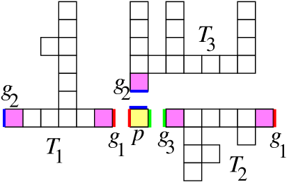
Figure 6: Assembling level-I components with three glues. In a first stage, $T_{1}$ gets assembled with pixel $p$ using glue $g_{1}$, leaving no exposed connections with glue type $g_{1}$ at $p$ or $T_{1}$. In a second stage, $T_{2}$ gets attached to $p$ using glue $g_{3}$. Because tiles and supertiles are non-rotatable, using glue type $g_{2}$ for T₃ does not interfere with the horizontal connections.

Level II. At the second level, we use corner pixels of degree two for further tree decomposition. We remove a pixel $t$ of degree two that separates $P_{W^{\prime}}$ into two subpolyominoes that both have almost the same number of corner pixels of degree two. Thus, the decomposition tree has again logarithmic height: now a node represents a corner pixel of degree $2$, while an edge corresponding to a straight line between two of them. By the same argument as above, we obtain a stage complexity of $\mathcal{O}(\log k)$ and a bin complexity of $\mathcal{O}(k)$ for all iterations of the second step.

As we use a new bin, we are allowed to use the same glues as for putting together the level-I pieces. None of these assembly steps is more complex than for level I, so we again conclude that three glues suffice.

Level III. We assemble the straight lines between connection pixels of degree $2$. For each strip, we reuse three glue types from the second step. For every type of strip (as defined above) we take six bins to build $1\times 2^{\ell}$ strips for some $\ell\in\mathbb{N}$. To build a specific strip, we proceed as follows. Let $m$ be the length of the strip; we build such a strip in one additional bin as in [4]. The individual segments for the strip are used from the bins for building strip types. Thus, we need $\mathcal{O}(\log m)$ stages for one strip; due to parallelism, this takes $\mathcal{O}(\log n)$ stages for assembling all straight strips.

For the overall backbone assembly, we use three glues, $\mathcal{O}(1)$ tiles and $\mathcal{O}(k)$ bins within $\mathcal{O}(\log n\cdot\log k)$ stages: we split at tree medians $\mathcal{O}(\log k)$ times, and use $\mathcal{O}(\log n)$ stages for each strip. ∎

Now we can establish our main result for $\tau=2$. The main idea is to construct the backbone using strength 2 for each glue in the construction of Lemma 3.4 and then flooding it by a specifically designed set of tiles $S$ with glues of strength 1, which is illustrated in Figure 7; see Figure 8 for the assembly process of flooding. These additional tiles are attached in a cooperative manner, i.e., by making use of two strength-1 glues for each attachment. Similar to the construction of Theorem 3.1, this ensures that precisely the pixels of the original polyomino are filled in.

Theorem 3.5.

Let $P$ be an arbitrary polyomino with $k$ vertices. Then there is a $\tau=2$ staged assembly system that constructs a fully connected version of $P$ in $\mathcal{O}(\log^{2}n)$ stages, with $6$ glues, $\mathcal{O}(1)$ tiles, $\mathcal{O}(k)$ bins and scale factor $3$.

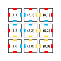
Figure 7: Glue chart for $3\times 3$ tiles for filling up the shape. The set $S$ of flooding tiles consists of the nine tiles shown in the figure. Blue glue $\stackrel{{\scriptstyle\wedge}}{{=}}g_{4}$, yellow glue $\stackrel{{\scriptstyle\wedge}}{{=}}g_{5}$ and red glue $\stackrel{{\scriptstyle\wedge}}{{=}}g_{6}$.

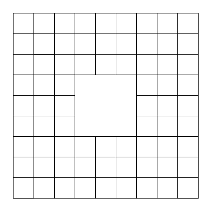
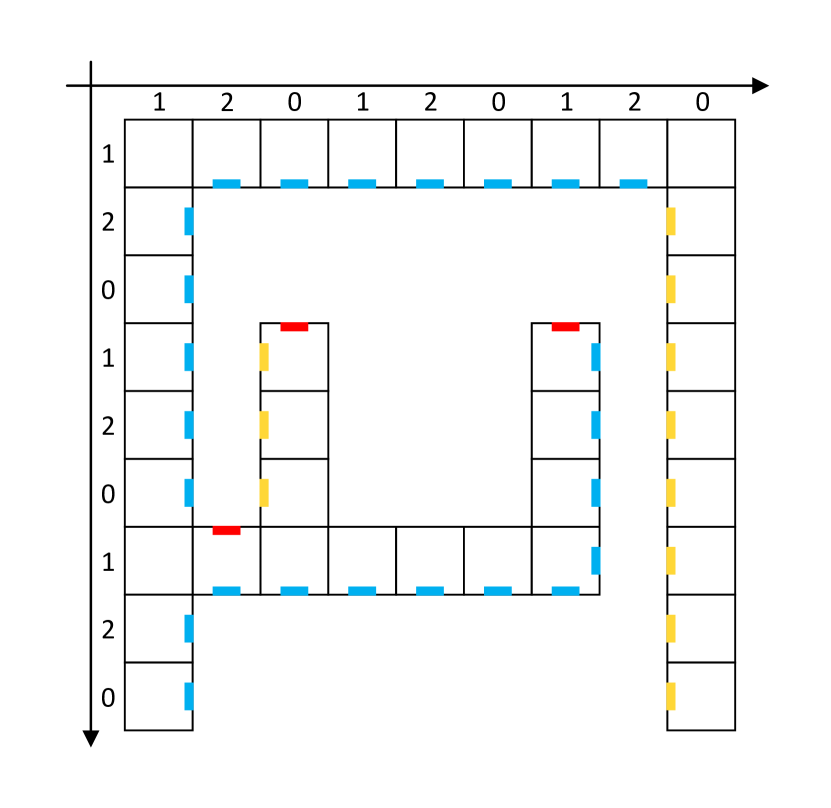
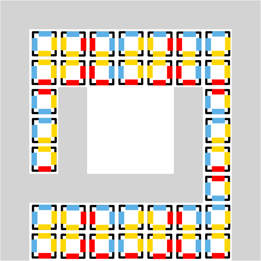
Figure 8: (Left) A polyomino $P^{3}$, obtained by scaling a polyomino $P$ with one hole by a factor of 3. (Middle) The backbone of $P^{3}$ with strength-1 glues assigned to the inside edges; note the coordinates modulo 3 and their correspondence to the glue chart. (Right) Filling up the backbone (shaded in grey) with the flooding tiles to assemble the polyomino.

Proof.

We assemble a polyomino $P^{3}$, obtained by scaling a polyomino $P$ by a factor of 3. Because of the scaling, all relevant coordinates of $P^{3}$ are multiples of 3. After assembling the backbone $B(P^{3})$ of $P^{3}$ (according to Lemma 3.4, making use of strength-2 glues $g_{1}$, $g_{2}$ and $g_{3}$), we consider the inside edges of $B(P^{3})$, which are the edges of pixels of $B(P^{3})$ that are incident to pixels in $P^{3}\setminus B(P^{3})$. Now the following is straightforward to verify from the construction of the backbone; refer to Figure 8 (Middle).

• All inside edges facing east separate pixels at $x$-coordinates 1 and 2 modulo 3, with the backbone pixel at 1 modulo 3.

• All inside edges facing south separate pixels at $y$-coordinates 1 and 2 modulo 3, with the backbone pixel at 1 modulo 3.

• All inside edges facing west separate pixels at $x$-coordinates 2 and 0 modulo 3, with the backbone pixel at 0 modulo 3.

• All inside edges facing north separate pixels at $y$-coordinates 0 and 1 modulo 3, with the backbone pixel at 1 modulo 3.

Now we specify the set of flooding tiles $S$; the idea is similar to the flooding tiles of Rothemund and Winfree [13] described in our Theorem 3.1. The mechanism is illustrated in Figure 7 and Figure 8.

$S$ consists of the set of nine tile types, shown in Figure 7. In addition to the three strength-2 glues used for assembling the backbone, we use three additional strength-1 glue types ($g_{4}$, $g_{5}$, $g_{6}$) that are assigned to the edges of tiles from $S$. Note the assignment modulo 3, corresponding to $x$- and $y$-coordinates as follows.

• A pixel of type $(1,1)$ gets glue type $g_{4}$ (east), $g_{4}$ (south), $g_{6}$ (west), $g_{6}$ (north).

• A pixel of type $(1,2)$ gets glue type $g_{4}$ (east), $g_{5}$ (south), $g_{6}$ (west), $g_{4}$ (north).

• A pixel of type $(1,0)$ gets glue type $g_{4}$ (east), $g_{6}$ (south), $g_{6}$ (west), $g_{5}$ (north).

• A pixel of type $(2,1)$ gets glue type $g_{5}$ (east), $g_{4}$ (south), $g_{4}$ (west), $g_{6}$ (north).

• A pixel of type $(2,2)$ gets glue type $g_{5}$ (east), $g_{5}$ (south), $g_{4}$ (west), $g_{4}$ (north).

• A pixel of type $(2,0)$ gets glue type $g_{5}$ (east), $g_{6}$ (south), $g_{4}$ (west), $g_{5}$ (north).

• A pixel of type $(0,1)$ gets glue type $g_{6}$ (east), $g_{4}$ (south), $g_{5}$ (west), $g_{6}$ (north).

• A pixel of type $(0,2)$ gets glue type $g_{6}$ (east), $g_{5}$ (south), $g_{5}$ (west), $g_{4}$ (north).

• A pixel of type $(0,0)$ gets glue type $g_{6}$ (east), $g_{6}$ (south), $g_{5}$ (west), $g_{5}$ (north).

Furthermore, pixels in the backbone get glues assigned to their inside edges, as follows.

• All inside edges facing east or south get strength-1 glue $g_{4}$.

• All inside edges facing west get strength-1 glue $g_{5}$.

• All inside edges facing north get strength-1 glue $g_{6}$.

Note that this assignment of $g_{4}$, $g_{5}$, $g_{6}$ to backbone pixels already happens when assembling the backbone, as described in Lemma 3.4; because these glues only face east/south, west, and north, respectively, and tiles and supertiles cannot be rotated, no bonding with these glues is possible between backbone pixels.

For filling the polyomino, we mix the nine kinds of flooding pixels (as shown in Figure 7) with the backbone supertiles in one bin. Now it is straightfoward to verify by induction that every pixel in $P^{3}\setminus B(P^{3})$ will get attached to the backbone by a cooperative sequence of assembly steps that each use two strenth-1 bonds; this is completely analogous to the technique described in our Theorem 3.1, with glues $g_{4}$, $g_{5}$ and $g_{6}$ being compatible at each step because of their coordinates modulo 3. Also analogous to the construction of squares in our Theorem 3.1, the converse holds: A pixel $p=(p_{x},p_{y})\not\in B(P^{3})$ can only be attached in this manner if first backbone pixels (say, $q$ and $r$) encountered when traveling from $p$ in two axis-parallel direction are met at inside edges, i.e., only when $p$ belongs to $P^{3}$. (See Figure 9.) This property only holds for pixels in $P^{3}$, implying that precisely $P^{3}$ gets assembled.

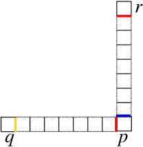
Figure 9: Attaching a pixel $p\not\in B(P^{3})$ to the backbone by a sequence of flooding tiles is only possible if the first backbone pixels encountered when traveling from $p$ in two axis-parallel direction are met at inside edges, i.e., only when $p$ belongs to $P^{3}$.

Overall, we have three glue types for building the backbone and three glue types for the flooding tiles for building the interior of the polyomino. Hence, we use a total of six glue types and $\mathcal{O}(1)$ tile types.

In total, we need $\mathcal{O}(\log^{2}n)$ stages, six glues, $\mathcal{O}(1)$ tiles and $\mathcal{O}(k)$ bins to assemble a fully connected polyomino, scaled by a factor 3 from the target shape. ∎

As noted before, the number of degree-3 corner pixels depends on the number of holes. We can describe the overall complexity in terms of $h$, the number of holes. For the special case of hole-free shapes, we can skip some steps, reducing the necessary number of stages. In particular, Corollary 3.6 follows from Theorem 3.5.

Corollary 3.6.

The stage complexity of Theorem 3.5 can be quantified in the the number of holes $h$ such we get a stage complexity of $\mathcal{O}(\log^{2}\,h+\log\,n)$. In particular, Theorem 3.5 gives a staged self-assembly system for hole-free shapes with $\mathcal{O}(\log\,n)$ stages, six glues, $\mathcal{O}(1)$ tiles, $\mathcal{O}(k)$ bins and a scale factor of 3.

4 Fully Connected Constructions for $\tau=1$

In this section we describe approaches for assembling fully connected polyominoes at temperature $\tau=1$.

4.1 Hole-Free Polyominoes, $\tau=1$

We present a system for building hole-free polyominoes. The main idea is based on [4], i.e., splitting the polyomino into strips. Each of these strips gets assembled piece by piece; if there is a component that can attach to the current strip, we create it and attach it.

Our geometric approach partitions the polyomino into rectangles and uses them to assemble the whole polyomino. Even for complicated shapes with many vertices, this number of rectangles is never worse than quadratic in the size of the bounding box; in any case we get a large improvement of the stage complexity.

We first consider a building block, see Figure 10. Originally a rectangle, its shape gets modified by tabs and pockets that fit together like key and lock. This is based on the jigsaw technique of [4], whose idea is to use the geometric shape for ensuring unique assembly. In our case tabs are $1\times 1$ or $1\times 2$ rectangles that are attached to the considered rectangle and pockets are $1\times 1$ or $1\times 2$ rectangles that are missing from the boundary of the considered rectangle.

Lemma 4.1.

A $2n\times 2m$ rectangle (with $n\geq m$) with at most two tabs at top and left side and at most two pockets at each bottom or right side (see Figure 10) can be assembled with $\mathcal{O}(\log n)$ stages, $9$ glues, $\mathcal{O}(1)$ tiles and $\mathcal{O}(1)$ bins at $\tau=1$.

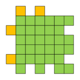
Figure 10: A rectangular shape (green) with tabs on top and left side (orange), and pockets on bottom and right side.

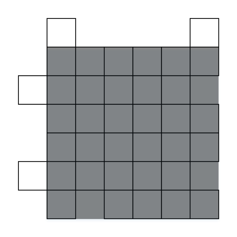
(a) Shaded in black is the original rectangle without tabs and pockets.

(b) Partition of the original rectangle into width-2 rectangles

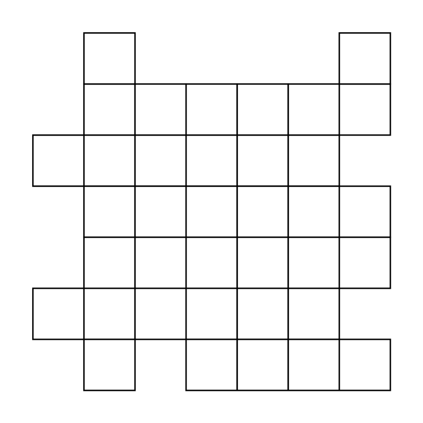
(c) The modified rectangle with tabs and pockets.

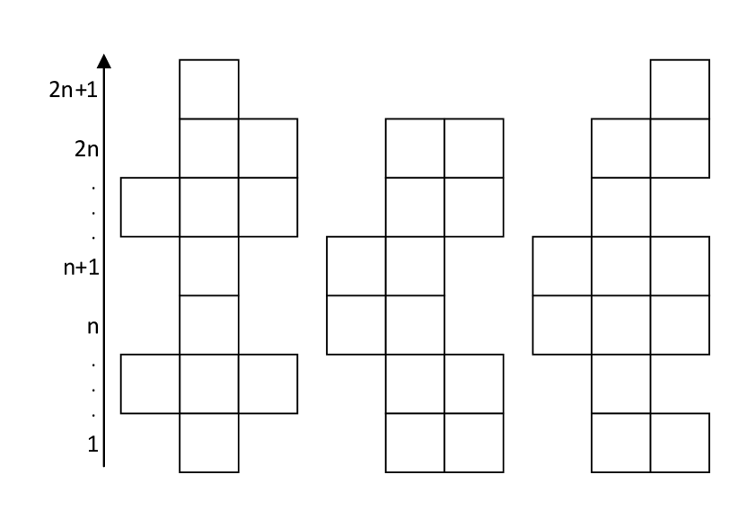
(d) Adding bulges, tabs and pockets to the width-2 rectangles. Note the coordinate labels for the rows.

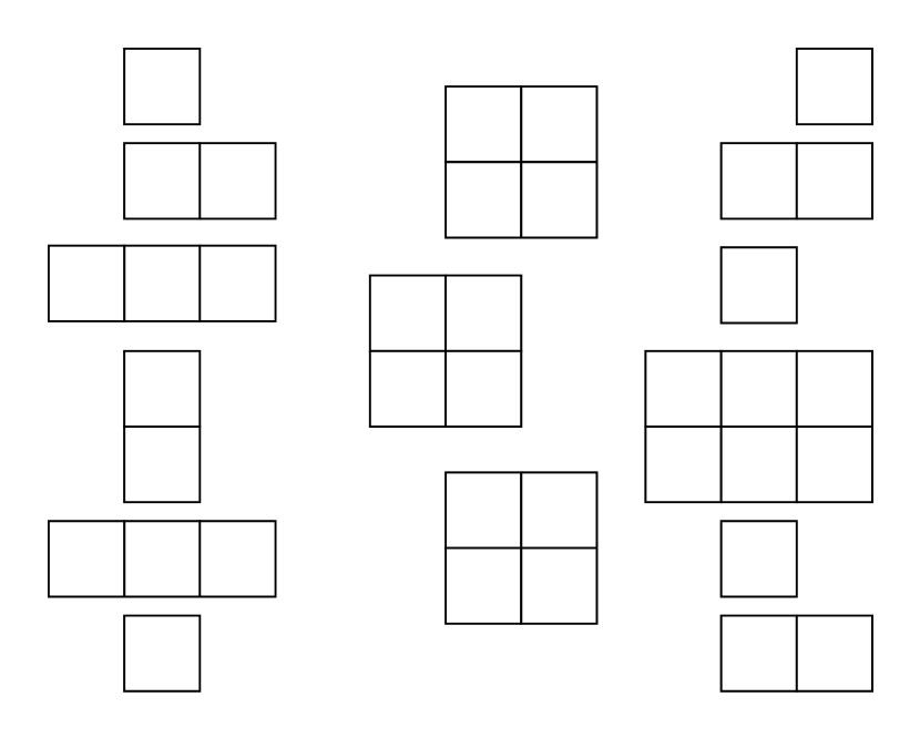
(e) Cutting the components horizontally. The left and the right component have tabs and pockets, the middle component has none.

Figure 11: Stepwise decomposition of a modified rectangle. The union of the dark shaded pixels indicates the initial rectangle whose shape is extended and reduced by tabs and pockets.

Proof.

Refer to Figure 11 for the overall construction. First consider the $2n\times 2m$ rectangle without any tabs or pockets (shaded dark in Figure 11(a)), which we partition into (vertical) rectangles of width 2 (see Figure 11(b)). Analogously, the modified rectangle shown in Figure 11(c) gets dissected into components, i.e., pieces that are joined by bulges in rows $n$ and $n+1$, in addition to the tabs and pockets from the shape we need to build (see Figure 11(d)). For assembly, we use glues on their sides like they are used in the jigsaw technique of [4]. Now every component has a maximum width of 3, even with the tabs. This allows us to use nine glues to create each component with attached tabs and pockets as follows.

A component without a tab or pocket (e.g., the middle component in Figure 11(e)) is cut between the $(n-1)$st and the $n$th row, as well as between the $(n+1)$st and the $(n+2)$nd row. Then we have two strips of width 2 and one $2\times 2$ square. The square can be assembled by brute force with desired glues on its sides. The strips can also be decomposed recursively like a $1\times n$ strip with desired glues on the sides. Thus, for this kind of component, nine glues suffice and the component is built within $\mathcal{O}(\log n)$ stages. Note that we need $\mathcal{O}(1)$ bins to store every possible component of this kind, i.e., they use one out of three possible glue triples on each side (compare to square assembly in [4]). Because the left side of a component uses completely different glue types than the right side, a component will never attach to itself.

A component with tabs and/or pockets (e.g., the left or right component in Figure 11(e)) is cut between rows, such that only components without tabs and pockets and at most four components with tabs and pockets exists. Note that the four components are either single tiles or lines of length at most three. The other components are either strips of width two or similar to the components above. Hence, we need at most $\mathcal{O}(\log n)$ stages to build the biggest component. Then we assemble all components by successively putting together pairs. We observe that this kind of component appears at most six times. Thus, we need six bins to store the components of this kind. Again the nine glues suffice.

Now we have all components in $\mathcal{O}(1)$ bins, so we can assemble the components in a pairwise fashion to the desired polyomino within $\mathcal{O}(\log n)$ stages. Overall, nine glues suffice, so we have $\mathcal{O}(1)$ tiles. ∎

Theorem 4.2.

Let $P$ be a hole-free polyomino with $k$ vertices. Then there is a $\tau=1$ staged assembly system that constructs a fully connected version of $P$ in $\mathcal{O}(\log^{2}n)$ stages, with $18$ glues, $\mathcal{O}(1)$ tiles, $\mathcal{O}(k)$ bins and scale factor $4$.

Proof.

We cut the polyomino $P$ with horizontal lines, such that all cuts go through reflex vertices of $P$, leaving a set of rectangles. If $V_{r}$ is the set of reflex vertices of the polyomino, we have at most $|V_{r}|=:k_{r}$ cuts and therefore $\mathcal{O}(k)$ rectangles. Consider the rectangle adjacency tree, i.e., a graph whose vertices are the rectangles and an edge connects two vertices if the corresponding rectangles have a side in common. Note that the resulting adjacency graph is a tree because $P$ has no holes. As shown in Figure 12(a), we find a rectangle $R$ that forms a tree median in the rectangle adjacency tree, i.e., a rectangle that splits the tree into connected components that each have at most half the number of rectangles.

Recursing over this splitting operation yields a tree decomposition of depth $\mathcal{O}(\log k)$. On the pieces, we use a scale factor of 2 for employing a jigsaw decomposition corresponding to [4].

(a) A splitting rectangle (orange) whose removal partitions the polyomino into components (green).

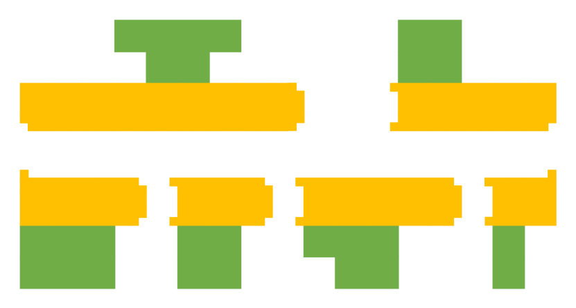
(b) Decomposition of the splitting rectangle.

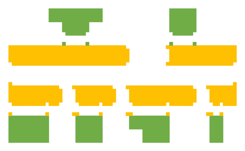
(c) Further decomposition of the resulting connected components.

Figure 12: Splitting operation by a median rectangle and further disassembly.

When considering a single split, the polyomino without $R$ decomposes into a number of connected components, corresponding to the green pieces in Figure 12(a). To assemble all of these components into the original polyomino, we employ another scale factor of 2, allowing us to split $R$ in half with a horizontal line, as shown in Figure 12(b). Each half is further subdivided vertically into jigsaw components, such that each component can connect to a part of $R$ independently from the others, as shown in Figure 12(c). For our purpose, we place the cuts for this subdivision such that they run along the leftmost side where a component of the chosen rectangle and its adjacent rectangle meet. When all components have been attached to some part of $R$, we can assemble both halves of $R$ and then put these two together. Doing this for all rectangles produces $\mathcal{O}(k_{r})$ new components. Hence, our decomposition tree has at most $\mathcal{O}(k_{r})=\mathcal{O}(k)$ leaves, where the leafs are rectangles that need $\mathcal{O}(\log n)$ stages for construction. This yields $\mathcal{O}(\log k\log n)$ stages overall; the rectangle components consume $\mathcal{O}(k)$ bins. Similar to assembling a square, we need nine glues to uniquely assemble all rectangles to the correct polyomino.

By construction, every rectangle component, i.e., a leaf of the decomposition tree, has at most four adjacent rectangle components, because we decompose a chosen rectangle until all of the rectangle components have at most four adjacent rectangles; its size is $2w\times 2h$ for some width $w$ and height $h$. The four adjacent components are all connected at different sides, so the left and upper side each have two tabs, while the right and lower side have two pockets. Thus, we can use the approach of Theorem 4.1 to assemble all rectangles with $9$ additional glues and $\mathcal{O}(1)$ bins for each rectangle component.

Overall, we have $\mathcal{O}(\log n)$ stages to assemble the $\mathcal{O}(k)$ rectangles with $\mathcal{O}(1)$ bins for each rectangle, plus $\mathcal{O}(\log^{2}n)$ stages to assemble the polyomino from the rectangles, for a total of $\mathcal{O}(\log^{2}n)$ stages and $\mathcal{O}(k)$ bins. For the rectangles we need nine glues, along with nine glues for the remaining assembly, for a total of 18 glues, with $\mathcal{O}(1)$ tile types. The overall scale factor is 4. ∎

With respect to later application in Theorem 4.4, we remark that the construction of Theorem 4.2 hinges on sufficient vertical thickness of the constructed polyomino; the scale factor is only used to guarantee this thickness.

Corollary 4.3.

Let $Q$ be a hole-free polyomino with $k$ vertices, such that $Q$ has vertical thickness at least 4, i.e., every maximal connected set of pixels in $Q$ with the same $x$-coordinate contains at least four elements. Then there is a $\tau=1$ staged assembly system that constructs a fully connected version of $Q$ in $\mathcal{O}(\log^{2}n)$ stages, with $18$ glues, $\mathcal{O}(1)$ tiles, $\mathcal{O}(k)$ bins.

The construction is identical to the one of Theorem 4.2; note that no scaling is necessary, as the vertical thickness suffices to allow the required horizontal splitting.

4.2 Polyomino with Holes, $\tau=1$

In this section we give staged assembly systems with temperature $\tau=1$ for arbitrary polyominoes that may have holes.

Theorem 4.4.

Let $P$ be an arbitrary polyomino with $k$ vertices. Then there is a $\tau=1$ staged assembly system that constructs in $\mathcal{O}(\log^{2}n)$ stages, with $20$ glues, $\mathcal{O}(1)$ tiles, $\mathcal{O}(n)$ bins a fully connected supertile $P^{6}$ that arises from $P$ by a scale factor of $6$.

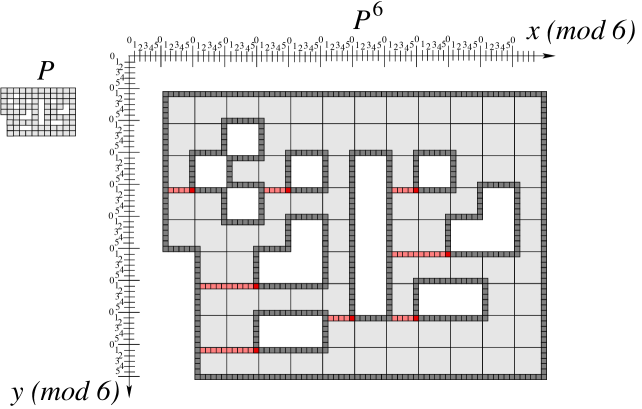
(a) An unscaled polymino $P$, the scaled $P^{6}$ and the construction of $S_{1}$. Bridges are shown in red.

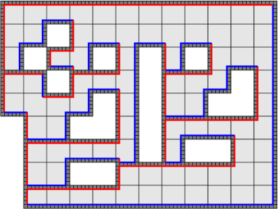
(b) The final pieces $S_{1}$ (dark grey) and $S_{2}$ (light grey), whith blue and red glue along the common boundary.

Figure 13: Partitioning $P^{6}$ into $S_{1}$ and $S_{2}$.

Proof.

From a high-level point of view, the approach constructs two supertiles $S_{1}$ and $S_{2}$ separately and finally glues them together, see Figure 13 for the overall construction. The first supertile $S_{1}$ consists of the boundaries of all holes, the boundary of the whole polyomino, and connections between these boundaries. The second supertile $S_{2}$ is composed of the rest of the polyomino. The scale factor of 6 guarantees that after removing the boundary pieces connected into $S_{1}$, $S_{2}$ is hole-free and has a thickness of 4, which allows employing the approach of Theorem 4.2 in the version of Corollary 4.3.

Partition of $P^{6}$ into $S_{1}$ and $S_{2}$: $S_{1}$ consists of all boundary pixels of $P^{6}$, connected by additional connections (“bridges”), such that the remainder $S_{2}=P^{6}\setminus S_{1}$ is connected and with vertical thickness four. To this end, consider the set of connected components of boundary pixels of $P^{6}$; one of them (say, $C_{0}$) contains the outside boundary, while the inside components (say, $C_{1},\ldots,C_{k}$) surround holes. Because of the scaling, every boundary pixel has $x$-cooordinate 0 or 1 (modulo 6) or $y$-cooordinate 0 or 1 (modulo 6). For each inside component $C_{i}$, consider its bottommost $p_{i}$ of the leftmost pixels. Because of the scaling, its $y$-coordinate is 1 modulo 6. For each inside component $C_{i}$, we add pixels to the left of $p_{i}$ until we hit a pixel of another boundary, say, $C_{j_{i}}$, thereby building a bridge $B_{i}$ from $C_{i}$ to $C_{j_{i}}$. Considering the coordinates of boundary pixels modulo 6, we conclude that no pixel of a bridge $B_{i}$ can be adjacent to a pixel of a boundary component other than $C_{i}$ and $C_{j_{i}}$. Therefore, the set of bridges induces a directed tree, with $C_{0}$ as the root node. As a consequence, the complement $S_{2}=P^{6}\setminus S_{1}$ is hole-free. Furthermore, the horizontal pieces of $S_{1}$ have $y$-coordinates 0 and 1 modulo 6, so $S_{2}$ has vertical thickness at least 4: Any pixel at the lower end of a boundary has $y$ coordinate 1 modulo 6, while a pixel at the upper end of a boundary has $y$ coordinate 0 modulo 6, so any vertical cut through $S_{2}$ must contain at least four pixels with $y$-coordinates 2, 3, 4, 5 modulo 6.

Assembling $S_{2}$. Because $S_{2}$ is hole-free and has vertical thickness 4, we can apply the approach of Theorem 4.2. During the construction of $S_{2}$, we guarantee that each northern and western face of the boundary of $S_{2}$ is marked by the red glue and each face from the eastern or southern boundary of $S_{2}$ by the blue glue, see Figure 13(b). To guarantee that these two additional glues do not interfere with the self-assembly of $S_{2}$, red and blue are not used in the approach from Theorem 4.2. Overall, we need $\mathcal{O}(\log^{2}(n))$ stages, $20$ glues and $\mathcal{O}(k)$ bins for the construction of $S_{2}$.

Assembling $S_{1}$. By construction of $S_{1}$, the bridges induce a tree between the boundary components. Hence, we can again use a median-based decomposition, i.e., recursively choose a boundary component that splits the tree into components that have at most half the numbers of components. Each boundary $C_{i}$, in turn, is again split into two chains that both contain at most half the number of pixels of $C_{i}$, see Figure 14. At the cutting pixels, we use two different glues for a unique attachment. For the staged self-assembly of the remaining chains, we apply the approach that is used to self-assemble strips in logarithmically many stages [4]. In particular, we split each chain recursively in the middle and mark the cutting pixels by a third glue type that is not used by both end pixels of the chain, see Figure 14. Finally, a fourth glue is needed for the attachment of a bridge $B_{i}$ to its parent component $C_{i}$ in the tree decomposition. This bridge, including its exit pixel at the other component $C_{j_{i}}$, can be constructed by applying the same approach that is used to construct the boundary components. Analogously to the construction of $S_{2}$, we mark the boundary of $S_{1}$ by red and blue, but now in the opposite direction: Each northern and western face of the boundary of $S_{1}$ is marked by the blue glue; each face from the eastern or southern boundary of $S_{1}$ is marked by the red glue, see Figure 13(b) and Figure 14. Again, red and blue are not allowed to be used for the construction of the supertile for $S_{1}$. Overall, we need $\mathcal{O}(\log^{2}(n))$ stages, $6$ glues and $\mathcal{O}(k)$ bins for the construction of $S_{2}$.

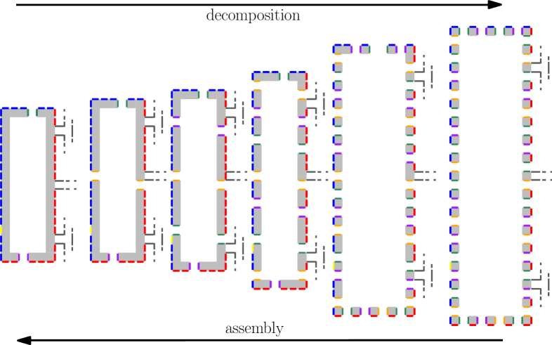
Figure 14: Recursive separation of a circle from $S_{2}$.

Putting together $S_{1}$ and $S_{2}$. Finally, it is straightforward to see that the geometry of $S_{1}$ and $S_{2}$ implies that they can only attach to each other in the canonical manner, making use of the red and blue glue, as shown in Figure 13(b).

Overall glue and stage complexity. As $S_{1}$ and $S_{2}$ are assembled in different bins and because all these glues bond after the construction of $S_{1}$ and $S_{2}$ we are allowed to make use of 6 glues from the construction of $S_{2}$ for the construction of $S_{1}$. Hence, overall we need $2+\max\{18,6\}=20$ glues for the construction of $P$. Thus, we obtain a total glue complexity of $20$, stage complexity $\mathcal{O}(\log^{2}(n))$, bin complexity $\mathcal{O}(k)$ with a scale factor of $6$. All bonds use temperature $\tau=1$.

∎

5 Future Work

Our new methods have the same stage and bin complexity as previous work on stage assemblies [4] and use just a small number of glues. Because the bin complexity is in $\mathcal{O}(k)$ for a polyomino with $k$ vertices, we may need many bins if the polyomino has many vertices. Hence, all our methods are excellent for shapes with a compact geometric description. This still leaves the interesting challenge of designing a staged assembly system with similar stage, glue and tile complexity, but a better bin complexity for polyominoes with many vertices, e.g, for $k\in\Omega(n^{2})$.

Another interesting challenge is to develop a more efficient system for an arbitrary polyomino. Is there a staged assembly system of stage complexity $o(\log^{2}n)$ without increasing the other complexities?

References

- [1] Z. Abel, N. Benbernou, M. Damian, E. D. Demaine, M. L. Demaine, R. Flatland, S. D. Kominers, and R. Schweller. Shape replication through self-assembly and RNAse enzymes. In ACM-SIAM Symposium on Discrete Algorithms (SODA), pages 1045–1064, 2010.
- [2] G. Aggarwal, Q. Cheng, M. H. Goldwasser, M.-Y. Kao, P. M. de Espanes, and R. T. Schweller. Complexities for generalized models of self-assembly. SIAM Journal on Computing, 34(6):1493–1515, 2005.
- [3] S. Cannon, E. D. Demaine, M. L. Demaine, S. Eisenstat, M. J. Patitz, R. T. Schweller, S. M. Summers, and A. Winslow. Two hands are better than one (up to constant factors). In Symposium on Theoretical Aspects of Computer Science (STACS), pages 172–184, 2013.
- [4] E. D. Demaine, M. L. Demaine, S. P. Fekete, M. Ishaque, E. Rafalin, R. T. Schweller, and D. L. Souvaine. Staged self-assembly: Nanomanufacture of arbitrary shapes with glues. Natural Computing, 7(3):347–370, 2008.
- [5] E. D. Demaine, M. L. Demaine, S. P. Fekete, M. J. Patitz, R. T. Schweller, A. Winslow, and D. Woods. One tile to rule them all: Simulating any tile assembly system with a single universal tile. In International Colloquium on Automata, Languages and Programming (ICALP), pages 368–379, 2014.
- [6] E. D. Demaine, S. P. Fekete, C. Scheffer, and A. Schmidt. New geometric algorithms for fully connected staged self-assembly. In 21st International Conference on DNA Computing and Molecular Programming (DNA’21), pages 104–116, 2015.
- [7] S. P. Fekete, J. Hendricks, M. J. Patitz, T. A. Rogers, and R. T. Schweller. Universal computation with arbitrary polyomino tiles in non-cooperative self-assembly. In ACM-SIAM Symposium on Discrete Algorithms (SODA), pages 148–167, 2015.
- [8] B. Fu, M. J. Patitz, R. T. Schweller, and R. Sheline. Self-assembly with geometric tiles. In International Colloquium on Automata, Languages and Programming (ICALP), pages 714–725. 2012.
- [9] J. E. Padilla, W. Liu, and N. C. Seeman. Hierarchical self assembly of patterns from the robinson tilings: DNA tile design in an enhanced tile assembly model. Natural Computing, 11(2):323–338, 2012.
- [10] J. E. Padilla, M. J. Patitz, R. T. Schweller, N. C. Seeman, S. M. Summers, and X. Zhong. Asynchronous signal passing for tile self-assembly: Fuel efficient computation and efficient assembly of shapes. International Journal of Foundations of Computer Science, 25(4):459–488, 2014.
- [11] S. H. Park, C. Pistol, S. J. Ahn, J. H. Reif, A. R. Lebeck, C. Dwyer, and T. H. LaBean. Finite-size, fully addressable DNA tile lattices formed by hierarchical assembly procedures. Angewandte Chemie, 118(5):749–753, 2006.
- [12] J. H. Reif. Local parallel biomolecular computation. In DNA-Based Computers, volume 3, pages 217–254, 1999.
- [13] P. W. K. Rothemund and E. Winfree. The program-size complexity of self-assembled squares (extended abstract). In ACM Symposium on Theory of Computing (STOC), pages 459–468, 2000.
- [14] K. Somei, S. Kaneda, T. Fujii, and S. Murata. A microfluidic device for DNA tile self-assembly. In 11th International Conference on DNA Computing and Molecular Programming (DNA 11), pages 325–335. 2006.
- [15] E. Winfree. Algorithmic self-assembly of DNA. PhD thesis, California Institute of Technology, 1998.