Obliquity or precession paces deglaciations over the last 2 million years: a Bayesian approach

Abstract

Milankovitch proposed that the orbital eccentricity, precession and obliquity of the Earth can influence the climate by modulating the summer insolation at high latitudes in the Northern hemisphere. Despite a great success of the Milankovitch theory in explaining the climate change over the Pleistocene, it is inconclusive with regard to which combination of orbital elements drove or paced the sawtooth $\sim$100-kyr glacial-interglacial cycles over the late Pleistocene. To explore the roles of different orbital elements in pacing the Pleistocene deglaciations, we model the ice-volume variations over the Pleistocene by combining simple ice-volume models with different orbital elements. The Bayesian formalism allows us to compare these models and we find that obliquity plays a dominant role in pacing the glacial cycles over the whole Pleistocene while precession only becomes important in pacing major deglaciations after the transition from the 100-kyr dominant to the 41-kyr dominant glacial-interglacial cycles (mid-Pleistocene transition). Unlike the traditional Milankovitch theory that the insolation at the summer solstice at $65^{\circ}$N drives the climate change, our results confirm previous studies that the climate response to the insolation is interconnected in multiple spatial and temporal scales. We also conclude that the mid-Pleistocene transition was shew with a time scale of about 100 kyr and the mid-point of the transition is about 710 kyr. We find that the geomagnetic field and orbital inclination variations are unlikely to pace the Pleistocene deglaciations. Our results are consistent with Milankovitch’s theory but also indicate a rather rapid change of the response of the climate system to the Northern hemisphere summer insolation during the mid-Pleistocene transition.

Keywords: Glacial cycles; Mid-Pleistocene; Obliquity; Precession; Orbital forcing; Hypothesis test

1 Introduction

Roughly over the past 2.5 Myr (the Pleistocene), the semi-periodic glaciation cycles dominate terrestrial climate change, mainly documented by climate records in the deep sea sediments and ice cores. Much of the variability of the climate change over the Pleistocene was claimed to be driven by the summer insolation (i.e. incoming solar radiation) at $65^{\circ}$N, which is the so-called Milankovitch’s theory (milankovitch41). Milankovitch also proposed that the climate change over different time scales are caused by the climate response to different orbital elements, including eccentricity, obliquity and precession. These orbital variations can potentially influence the climate and thus are one type of climate forcing, i.e. orbital or Milankovitch forcing. Many previous studies have confirmed the correlation between Milankovitch forcing and the Pleistocene climate change by spectral analyses of two paleoclimatic time series derived from deep-sea sediments (hays76; shackleton73; kominz79). by analyzing the power spectrum of the climate variations by his conclusion by studying the , the ice-volume variations over the past 2 Myr have periods around 23 kyr and 41 kyr which can be can be explained by The summer insolation at modulated by the change of eccentricity, precession and obliquity of the Earth’s orbit. can be explained by a linear response of the climate system to the insolation ( modulated by precession, obliquity and eccentricity of the Earth’s orbit (hays76; berger78; imbrie92). These About 0.8 Myr ago (the mid-Pleistocene period), the pattern of climate changes shifted from 41-kyr dominant to 100-kyr dominant glacial-interglacial cycles. The non-100-kyr variations in the climate change can also be successfully explained by the classical Milankovitch theory which claims that the summer insolation at high latitudes is associated with terrestrial climate change (milankovitch41).

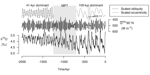
Figure 1: The $\delta^{18}$O record (solid) stacked by lisiecki05 compared with obliquity (dashed) and eccentricity (dotted) calculated by laskar04 over the past 2 Myr. The grey bar represents the MPT extending from -1250 kyr to -700 kyr (clark06). The $\delta^{18}$O variations are dominated by 41-kyr and 100-kyr cycles before and after the MPT, respectively.

However, there are two types of difficulties in explaining the 100-kyr cycles based on Milankovitch theory: the transition from the 100-kyr world to the 41-kyr world and the forcings and response mechanisms of generating 100-kyr sawtooth variations (see imbrie93, huybers07 and lisiecki10 for details). On the one hand, the onset of 100-kyr power at the mid-Pleistocene transition (MPT) without a corresponding change in the insolation forcing. On the other hand, a linear climate response to the $\sim$100-kyr eccentricity variations is not significant enough to generate the 100-kyr power in the climate change, particularly in ice volume variations. In addition, the 400-kyr dominant period in eccentricity variations does not appear in changes in the late Pleistocene ice volume (imbrie80). Further, the eccentricity cycles and the 100-kyr climatic variations are anti-correlated, notably in marine isotope stage (MIS) 11 (imbrie93; parrenin03).

Different forcings and response mechanisms are proposed to solve the above problems. For example, the $\sim$100-kyr sawtooth glacial-interglacial cycles are claimed to be caused by eccentricity modulated precession (raymo97; lisiecki10), obliquity cycle skipping (huybers05; liu08), or internal oscillations phase-locked by Milankovitch forcing (saltzman84; tziperman06). The MPT is attributed either to an abrupt change of the climate system (raymo97; paillard98; honisch09; clark06) or a variable climate response to Milankovitch forcing (saltzman93; huybers09; lisiecki10; imbrie11). Apart from the above mechanisms based on Milankovitch forcings, there are also other studies proposing the glacial cycles are caused by the accretion of interplanetary dust when the Earth crosses the invariant plane (muller97) or by the cosmic ray influx modulated by the geomagnetic paleointensity (or GPI; christl04; courtillot07).

The above models always consist of two components: forcings and climate responses. Our current work aims to compare different forcings based on a simple scenario of climate response for the Pleistocene glacial terminations. We adopt the simple response/pacing model given by huybers05 and combine it with different forcings to predict the glacial terminations which are identified from different $\delta^{18}$O records (huybers07; huybers11). Unlike most conceptual models, these models do not try to describe the physical mechanisms of the climate response to external forcings. They aim instead to investigate the roles of different external forcings in determining some key features in proxy variations such as glacial terminations. These conceptual models are also called statistical models (crucifix12).

Instead of using p-values to reject null hypotheses (huybers05; huybers11), we properly compare all models/hypotheses on an equal footing in the Bayesian framework. Through assessing the overall plausibility of models, the Bayesian inference favors simple models which can explain the data without fine-tuning their parameters rather than complex models which can be highly tuned to over-fit the noise contaminated data (see kass95; spiegelhalter02; bailer-jones09 for details).

This paper is organized as follows. We introduce the 100-kyr problem and our approach to compare different climate forcings in section 1. Then we choose different stacked $\delta^{18}O$ records and derive glacial terminations from them in section 2. In section 3, we summarize the Bayesian inference method and introduce the evidence or Bayes factor as a metric for model comparison. In section 4, we build models based on orbital elements and GPI proxies to predict the Pleistocene glacial terminations. In section 5, these models are compared using the Bayesian method for different data sets and time scales. We perform a test of sensitivity of the results to model parameters and time scales in section 6. Finally, we discuss the results and conclude in section 7.

2 Data

2.1 $\delta^{18}$O with depth-derived age model

The climate of the past can be reconstructed from proxies such as isotopes which are recorded in ice cores, deep-sea sediments, etc.. For example, air bubbles in ice cores are atmosphere samples from the past and can be analyzed for CO₂ concentrations. These are sensitive to the temperature of the atmosphere, so the history of Earth’s surface temperature can be reconstructed from ice core records. The longest ice core can trace the climate history back to about 800 kyr (augustin04). In order to reconstruct the climate change over the last 2 Myr, the $\delta^{18}$O proxy (i.e. the ratio between ¹⁸O and ¹⁶O relative to a standard isotope composition) recorded in foraminifera fossils (include species of benthos and plankton) in ocean sediment cores is used due to its sensitivity to the deep ocean temperature and ice volume in the past.

To calibrate $\delta^{18}$O measurements and assign ages to depths (or age model) of sediment cores, researchers either assume a constant globally averaged sedimentation rate or a constant phase relationship between $\delta^{18}$O measurements and an insolation forcing based on Milankovitch theory (see huybers04 for details). The former is called depth-derived age model (huybers04; huybers07) which are always used to test Milankovitch theory (huybers05; lisiecki10; huybers11). On the contrary, the later calibration method is named “orbital tuning” (imbrie84; martinson87; shackleton90) and is not appropriate for testing theories related to Milankovitch forcings because it assumes a link between $\delta^{18}$O variations and orbital forcings.

huybers07 (hereafter H07) have stacked and averaged twelve benthic and five planktic $\delta^{18}$O records to generate three $\delta^{18}$O global records: average of all $\delta^{18}$O records (“HA” data set); average of the benthic records (“HB” data set) and average of the planktic records (“HP” data set). Apart from these three data sets, we also use the orbital-tuned benthic $\delta^{18}O$ stacked by lisiecki05 (defined as “LR04” data set) despite its orbital assumptions. In addition, the LR04 record is re-calibrated by H07 to generate a tuning-independent LR04 data set (defined as “LRH” data set and refer to the supplementary material of H07 for details).

All the above $\delta^{18}$O records over the past 2 Myr are normalized and shown in Figure 2. We can see that the sawtooth 100-kyr glacial-interglacial cycles become significant over the late Pleistocene while 40-kyr cycles dominate the climate change over the early Pleistocene. All records show gradual glaciations and abrupt deglaciations over the late Pleistocene. Hereafter, in the context without mentioning the MPT, the late Pleistocene means a period ranging from -1 Myr to 0 Myr, and the early Pleistocene means a period ranging from -2 Myr to -1 Myr.

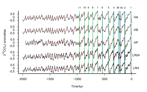
Figure 2: The $\delta^{18}$O data sets with ages determined by extended depth-derived age-model (H07) and the corresponding identified deglaciation events (red error bars). The error bars denote one sigma error in the times of deglaciation events. The DD terminations are denoted by dashed lines while the ML/MS terminations are denoted by dotted lines. The 11 terminations are denoted by numbers and termination 3 is split into two events.

2.2 Identification

Instead of using the full $\delta^{18}$O times series, we identify the deglaciation events or glacial terminations from each time series because our goal is to find the plausible forcing which can determine or pace the timing of these features. Following H07, a deglaciation event is identified when a local maximum and the following minimum have a difference in ice volume larger than one standard deviation of the whole ice volume. The time and time uncertainty of a deglaciation event is the mid-point and half width in time of the maximum-minimum pair, respectively. In order to identify sustained events in all data sets, the $\delta^{18}$O records are first filtered with moving-average (or “Hamming”) filters: HA and HB are filtered with a 7 kyr filter, HP and LRH are filtered with a 11 kyr filter, and LR04 is filtered with a 9 kyr filter, respectively. As a result, there are 20 deglaciation events during early Pleistocene period and 16 deglaciation events during late Pleistocene period for HA, 20 and 16 for HB, 21 and 16 for HP, 20 and 17 for LR04, 20 and 16 for LRH. The age uncertainties of these deglaciation events are denoted by error bars in Figure 2.

However, H07’s method cannot efficiently identify the major late-Pleistocene deglaciation events which have the termination features defined by broecker84; raymo97b because it identifies all Pleistocene deglaciations with one method, disregarding the difference between early and late Pleistocene terminations. This is evident from the excessive number of late-Pleistocene deglaciation events compared with the 11 major terminations extensively studied in the literature. To distinguish the terminations identified using H07’s method and these 11 terminations, we define major or well-studied glacial terminations as the 11 late-Pleistocene deglaciations which are frequently studied in literatures and with the specific termination characteristics given by (broecker84). Among these terminations, termination 3 is usually split into two events: 3a and 3b, and thus the major terminations actually contain 12 events (see Fig. 2).

The times of the 12 terminations from different literatures are collected by huybers11 in his supplementary material. Based on his Table S2, we define another three data sets of terminations:

• DD: termination times and corresponding uncertainties estimated from the depth-derived timescale in H07,

• MS: each termination with time and time uncertainty respectively equal to the median and standard deviation of different termination times for each event given in the literature,

• ML: termination times the same as those in the MS data set but with larger uncertainties by adding the time uncertainties of the depth-derived time scales in quadrature with the corresponding uncertainties in the MS data set.

The above three sets of major terminations are shown by vertical bars in Figure 2.

Finally, we define three hybrid data sets particularly for climate models which predict the climate change over the last 2 Myr and the MPT. Considering that the HA data set is a stack of both benthic and planktic records, we combine the early-Pleistocene deglaciation events identified from the HA data set and late-Pleistocene terminations from the DD, ML and MS data sets to generate HADD, HAML, HAMS data sets, respectively.

Before using these terminations to test models in section 5, each termination is treated as a Gaussian probability distribution with the mean and standard deviation equal to the time and time uncertainty of the termination respectively. Thus the terminations in a data set are treated as a Gaussian sequence which will be interpreted from a Bayesian perspective in the following section.

3 Bayesian inference

A Bayesian method is used to compare different models for different data sets, with advantages of proper accounting for model complexities and data uncertainties. The posterior probability is calculated according to the Bayes’ rule:

$$P(M|D)=\frac{P(D|M)P(M)}{P(D)},$$ (1)

where $P(M|D)$ is the posterior of model M given data D, $P(D|M)$ is the marginalized likelihood or evidence, $P(M)$ is the prior of model M, and $P(D)$ is a normalization factor. Model M has parameters $\boldsymbol{\theta}$, and thus the above formulae can be rewritten as

$$P(M|D)=\frac{\int P(D|\boldsymbol{\theta},M)P(\boldsymbol{\theta}|M)P(M)d\boldsymbol{\theta}}{P(D)}.$$ (2)

Assuming a constant $P(M)$, the posterior ratio of two models, $M_{1}$ and $M_{2}$, is

$$\frac{P(M_{1}|D)}{P(M_{2}|D)}=\frac{P(D|M_{1})}{P(D|M_{2})}=\frac{\int P(D|\boldsymbol{\theta_{1}},M_{1})P(\boldsymbol{\theta_{1}}|M_{1})d\boldsymbol{\theta_{1}}}{\int P(D|\boldsymbol{\theta_{2}},M_{2})P(\boldsymbol{\theta_{2}}|M_{2})d\boldsymbol{\theta_{2}}}.$$ (3)

The above posterior or evidence ratio is also named Bayes factor. The integral of above equations, $P(D|\boldsymbol{\theta},M)$, is the likelihood and $P(\boldsymbol{\theta}|M)$ is the parameter prior probability distribution of model M. If different priors of model $M_{1}$ and $M_{2}$ are adopted for reasons such as the Occam’s razor, a ratio $P(M_{1})/P(M_{2})$ is expected to be included in the above formulae of Bayes factor. To derive the Bayes factor, the likelihood and evidence are calculated as follows.

To account for age uncertainties of terminations, we interprete the measured data using a measurement model (see bailer-jones11; bailer-jones11b for details) which is

$$P(t_{j}|\sigma_{j},\tau_{j})=\frac{1}{\sqrt{2\pi}\sigma_{j}}e^{(t_{j}-\tau_{j})^{2}/2\sigma_{j}^{2}},$$ (4)

where $t_{j}$ is the measured time of termination $j$ with corresponding measurement uncertainty $\sigma_{j}$, and $\tau_{j}$ is the true termination time. Followingbailer-jones11; bailer-jones11b, we consider the data to be $D_{j}=t_{j}$ rather than $D_{j}=(t_{j},\sigma_{j})$ and implicitly condition on the measurement uncertainty, $\sigma_{j}$. Thus the likelihood appeared in Eqn. 2 is $P(D|\sigma,\boldsymbol{\theta},M)$ instead, where $\sigma=\{\sigma_{j}\}$. The measurement model for data $D=\{t_{j}\}$ is actually the normalized Gaussian sequence defined in section 2.

If the data $D$ contain N events which have independent times of occurrence and time uncertainties, the probability of observing the data $D=\{t_{j}\}$ or likelhood is

$$P(D|\sigma,\boldsymbol{\theta},M) = \prod\limits_{j}P(t_{j}|\sigma_{j},\boldsymbol{\theta},M)$$

$$= \prod\limits_{j}\int_{\tau_{j}}P(t_{j}|\sigma_{j},\tau_{j})P(\tau_{j}|\boldsymbol{\theta},M)d\tau_{j},$$

where $P(t_{j}|\sigma_{j},\boldsymbol{\theta},M)$ is the likelihood for event $j$ or event likelihood, which is a convolution of the measurement model $P(t_{j}|\sigma_{j},\tau_{j})$ and the predicted probability of the occurrence time for one event $P(\tau_{j}|\boldsymbol{\theta},M)$. In the following section, we will define $P(\tau_{j}|\boldsymbol{\theta},M)$ as a Gaussian function and thus $P(\tau|\boldsymbol{\theta},M)$ ($\tau={\tau_{j}}$) is a series of Gaussions (see the lower panel of Fig. 5). Thus the event likelihood is actually a convolution between a Gaussian probability distribution in a Gaussian sequence and another Gaussian sequence which are illustrated in the lower panel of Fig. 5.

The evidence is obtained by marginalizing the likelihood over the prior distribution

$$P(D|\sigma,M)=\int_{\boldsymbol{\theta}}P(D|\sigma,\boldsymbol{\theta},M)P(\boldsymbol{\theta}|M)d\boldsymbol{\theta}.$$ (6)

The evidence can be calculated using Monte Carlo methods through sampling from the parameter prior probability distribution, $P(\boldsymbol{\theta}|M)$, calculating the likelihood $P(t|\boldsymbol{\theta},M)$ for each, and averaging all likelihoods.

Based on the criterion given by kass95, if the evidence ratio (or Bayes factor) of model 1 and model 2 are larger than a factor of 10, we conclude that model 1 is better favored than model 2. Unlike using p-value as a metrics to assess the plausibility of a model, Bayesian inference can properly take into account the complexity of a model by marginalizing the likelihood over the prior. In contrast to the frequentist statistics, Bayesian inference can appropriately account for timing errors of the climate data and the parameter uncertainties in the model. This method is already applied in many solar-terrestrial studies (feng13; feng14).

4 Models

The “sawtooth” variations of the global ice volume (also present in other climate proxies) and the significant 100-kyr cycles over the late Pleistocene require a non-linear response of the climate system to Milankovitch forcings which include precession, obliquity and eccentricity. This can be modeled by simple conceptual models which combine different feedback mechanisms such as ice-albedo feedback (tziperman03) and CO₂ feedback (saltzman90). Another modeling approach is to construct a differential model of ice volume with some parameters changing with thresholds of the ice volume (gildor00; tziperman03; ashkenazy04) or the Milankovitch forcing (paillard98; parrenin03). These models can explain the sawtooth structure and even MPT to various degrees of success through transitions between different equilibria or bifurcations generated from the non-linear climate system.

However, each of these methods adopts a different climate mechanism to generate a non-linear climate response to forcings. Each assumes a dependence or independence of the climate change on Milankovitch forcings, either the summer insolation at 65^∘ N (i.e. classical Milankovitch theory) or combinations of orbital elements, over the Pleistocene. Here, we test these assumptions as huybers05 and huybers11 did, but now, within a Bayesian framework. To do this, we (1) introduce different climate forcings (section 4.1); (2) predict the 100-kyr sawtooth structure and the MPT by response or pacing models which truncate a linearly increasing ice volume with a threshold modulated by different forcings (section 4.2); (3) identify glacial terminations from these pacing models and compare them with the terminations derived from the data (section 4.3). In sum, we define different forcing models, include them into pacing models from which we generate termination models to predict terminations derived from the data, and compare termination models in a Bayesian framework (section 3).

4.1 Forcing models

The solar insolation influences the climate by heating the lower atmosphere, changing the ice volume through modifying by the ice accumulation rate, and modulating the CO₂ concentration in the atmosphere by altering the rate of CO₂ dissolution in the ocean (saltzman90). These climate changes are claimed to be more sensitive to the summer insolation at high latitudes because the temperature in continental areas is critical for ice melting in the Northern Hemisphere summer (milankovitch30). The summer insolation at high latitudes depends on the geometry of the Earth’s orbit and the inclination of Earth’s spin axis, and thus depends on eccentricity, precession and obliquity.

However, the climate response to these three semi-periodic orbital variables has different time scales, and insolation variations at different latitudes and seasons vary differently with these orbital elements. It is therefore necessary to combine these orbital variables to form a compound forcing model (imbrie80; huybers11; crucifix13). The forcing models based on normalized time-varying eccentricity ($f_{\rm E}(t)$), precession ($f_{\rm P}(t)$), obliquity ($f_{\rm T}(t)$) and combinations thereof are described as follows

$$\begin{array}[]{l}\displaystyle f_{\rm E}(t)=e(t)\\ \displaystyle f_{\rm P}(t)=e(t)\sin(\omega(t)-\phi)\\ \displaystyle f_{\rm T}(t)=\epsilon(t)\\ \displaystyle f_{\rm EP}(t)=\alpha^{1/2}f_{\rm E}(t)+(1-\alpha)^{1/2}f_{\rm P}(t)\\ \displaystyle f_{\rm ET}(t)=\alpha^{1/2}f_{\rm E}(t)+(1-\alpha)^{1/2}f_{\rm T}(t)\\ \displaystyle f_{\rm PT}(t)=\alpha^{1/2}f_{\rm P}(t)+(1-\alpha)^{1/2}f_{\rm T}(t)\\ \displaystyle f_{\rm EPT}(t)=\alpha^{1/2}f_{\rm E}(t)+\beta^{1/2}f_{\rm P}(t)+(1-\alpha-\beta)^{1/2}f_{\rm T}(t),\end{array}$$ (7)

where $e(t)$, $\epsilon(t)$ and $e(t)\sin(\omega(t)-\phi)$ are the time-varying eccentricity, obliquity and precession index, respectively. The precession index is also called climatic precession because it directly relates to insolation. In the precession index, $\omega(t)$ is the angle between perihelion and the moving vernal equinox, and $\phi$ is a free parameter controlling the phase of precession. We adopt the variations of these three orbital elements over the past 2 Myr as calculated by laskar04. Finally, $\alpha$ and $\beta$ are contribution factors which determine the relative contribution of each component in the compound models: $0\leq\alpha\leq 1$ and $0\leq\beta\leq 1$. All variables in compound models are normalized to zero-mean and unit variance before combination. Apart from these models, we also model the classical Milankovitch forcing (i.e. daily-averaged insolation at 65^∘N on July 21) as

$$f_{\rm Ins}(t)=\bar{Q}_{\rm day}(e(t),e(t)sin(\omega(t)-\phi),\epsilon(t)).$$ (8)

$\bar{Q}_{\rm day}$ can be calculated from the values of orbital elements given by laskar04.

Although conceptual models based on Milankovitch forcing achieve a great success in explain the precession and obliquity related cycles in the climate change over the Pleistocene (hays76; imbrie84; imbrie93), the 100-kyr problem (see section 1) has motivated scientists to propose other climate forcings, such as cosmic rays (svensmark97; kirkby04), Earth’s orbital inclination with respect to the invariant plane (muller97), the geomagnetic field (courtillot07; knudsen08) and solar activity (sharma02). Here we build two forcing models based on the variations of Earth’s orbital inclination and geomagnetic field paleointensity (GPI). We ignore the cosmic ray forcing and solar activity forcing because the history of cosmic ray influx and the solar activity cannot be accurately reconstructed from the concentrations of cosmogenic isotopes such as ¹⁰Be over a time scale longer than 1 Myr (bard06).

Although the orbital inclination relative to the invariant plane also has a $\sim$100-kyr variance, it is not included into Milankovitch theory because it cannot directly change the insolation at the top of Earth’s atmosphere. However, muller97 proposed that the insolation at the Earth’s surface can be modulated by an increase in the amount of interplanetary dust or meteoroids when the Earth crosses the invariant plane. To test this hypothesis, we model the inclination-based forcing as

$$f_{\rm Inc}(t)=\eta(t),$$ (9)

where $\eta(t)$ is orbital inclination. We will use the orbital inclination calculated by quinn91 and adapted for climatic usage by muller97.

The geomagnetic field on the Earth can influence the climate through changing cosmic-ray induced nucleation of clouds (courtillot07). We model this forcing as

$$f_{\rm G}(t)=G(t),$$ (10)

where $G(t)$ is the normalized GPI time series. We will use the GPI record collected by channell09.

All forcing models and corresponding prior distributions over their parameters (defined as “forcing parameters”) are shown in Table 1. For the precession model, we set $\phi=0$ to treat precession according to the classical Milankovitch theory that a high summer insolation in the Northern Hemisphere tend to trigger a deglaciation. Because we don’t have any prior knowledge about the value of contribution factors, compound models have uniform prior distributions over the interval of $[0,1]$ for these contribution factors. Following huybers05 and huybers11, we adopt positive contribution factors because eccentricity, precession and tilt contribute positively to the daily average insolation at summer solstice. However, we will test this by reversing the sign of the variations of these orbital elements and assigning time lags to different forcing models in section 6. In Table 1, all parameters are treated as dimensionless variables after setting the time unit as 1 kyr and the ice volume unit as unit 1. Fig. 3 shows the normalized forcing models with a single component. All forcing models will be included in pacing models and corresponding termination models in the following sections. Hereafter, for each forcing model, the corresponding pacing and forcing models share the same name which is shown in the first column of Table 1.

Table 1: The termination models and corresponding forcing models and the uniform prior distributions over forcing parameters. Except for the Periodic model, all termination models without any trend component have common parameters which vary uniformly within the following intervals: $0<b<0.1$, $0<v_{0}<90\gamma$, $90\gamma<h_{0}<130\gamma$ and $15\gamma<a<35\gamma$, where $\gamma$ can be either 0.4 or 1. For the periodic model, $a$ is zero and $h_{0}$ has a uniform prior distribution over $70\gamma<h_{0}<110\gamma$.

Termination models	Description	Forcing models	Uniform prior distribution over forcing parameters
Periodic	100-kyr pure periodic model	None	None
Eccentricity	Eccentricity	$f_{\rm E}(t)$	None
Precession	Precession	$f_{\rm P}(t)$	$\phi=0$
Tilt	Tilt or obliquity	$f_{\rm T}(t)$	None
EP	Eccentricity plus Precession	$f_{\rm EP}(t)$	$0\leq\alpha\leq 1$, $\phi={\rm 0}$
ET	Eccentricity plus Tilt	$f_{\rm ET}(t)$	$0\leq\alpha\leq 1$
PT	Precession plus Tilt	$f_{\rm PT}(t)$	$0\leq\alpha\leq 1$, $\phi=0$
EPT	Eccentricity plus Precession plus Tilt	$f_{\rm EPT}(t)$	$0\leq\alpha,\beta\leq 1$ and $\alpha+\beta\leq 1$, $\phi=0$
Insolation	Insolation	$f_{\rm Ins}(t)$	None
Inclination	Inclination	$f_{\rm Inc}(t)$	None
GPI	Geomagnetic paleointensity	$f_{\rm G}(t)$	None

Figure 3: Normalized single-component forcing models. The values of eccentricity, precession and obliquity are simulated by laskar04, the orbital inclination relative to the invariant plane is from muller97, and the GPI record is from channell09.

4.2 Pacing models

We use the deterministic model adapted from the stochastic model introduced by huybers05 to model the ice volume at time $t$ as

$$v_{t}=v_{t-1}+\eta_{t}\quad\quad\text{and if }v_{t}>h_{t}\text{ then terminate},$$ (11)

with

$$h_{t}=h_{0}-af_{t},$$ (12)

where $v_{t}$ is the ice volume which increases by a value of $\eta_{t}$ until it passes a threshold $h_{t}$ which is modulated by a climate forcing $f_{t}$. The increment $\eta_{t}$ is 1 ice-volume unit when the threshold is not passed; otherwise, the increment has such a value that the ice volume can linearly decrease to 0 over 10 kyr. Here we define the Periodic model as pacing models with a constant threshold which is not modulated by any forcing model. This model predict a pure periodic glacial cycles with a single period of $(h_{0}+10)$ kyr.

The above pacing model does not aim to physically model the nonlinear climate response to Milankovitch forcing, but just to reproduce the sawtooth structure with a simple function. The predicted time of glaciation termination is determined by the initial ice-volume $v_{0}$ and the threshold $h_{t}$. A pure periodic pacing model is generated by adopting a constant threshold, $h_{t}=h_{0}$ (see Fig. 4). Other pacing models are generated by modulating the threshold by different forcing models (see Eqn. 12). These pacing models have common pacing parameters: initial ice volume $v_{0}$, threshold constant $h_{0}$ and forcing modulation factor $a$. Because the time step and ice-volume increment are constants, the average period of semi-periodic ice-volume variations is determined by $h_{0}$ if the threshold is not modulated by forcings. This relationship between $h_{0}$ and the average period in ice volume variations is clearly illustrated by the $h_{0}$-determined saw-tooth peroidic variations in Fig. 4. When forcings are added onto the constant threshold, the average period of ice volume variations would decrease by an amount of $\sim a$ ice volume units, due to the effect that the ice volume accumulation tend to terminate at forcing maxima. To be specific, the average period of ice volume anomalies is $\sim(h_{0}+10-a)$ kyr.

Considering the linear relationship between $h_{0}$, $a$ and periods in ice volume variations, a hyperparameter $\gamma$ is required to change the prior distributions of $h_{0}$ and $a$ to allow a reproduction of $\sim$41-kyr cycles over the early Pleistocene and $\sim$100-kyr cycles over the late Pleistocene. Thus we define uniform prior distributions of $v_{0}$, $h_{0}$ and $a$ over the following intervals: $0<v_{0}<90\gamma$, $90\gamma<h_{0}<130\gamma$ and $15\gamma<a<35\gamma$, where $\gamma=0.4$ when we model $\sim$41-kyr cycles and $\gamma=0.4$ when we model $\sim$100-kyr cycles. The range of $v_{0}$ is just the range of the ice-volume variation while the mean values of the prior distributions of $h_{0}$ and $a$ with $\gamma=1$ are the optimal values obtained by huybers11. In section 6, we will change these prior distributions to check whether our results are sensitive to them.

Figure 4: A schematic view of different trend functions for $h_{0}$: constant (red), linear (green) and sigmoid trend (other colors). Examples of pacing models with constant threshold $h_{0}=30$ and $h_{0}=90$ are shown in grey lines here.

However, because the threshold constant $h_{0}$ can only model variations with one period, the pacing model defined by Eqn. 11 and 12 is not capable to model the climate change over both the early and late Pleistocene and thus the MPT within a single set of parameters (see Fig. 4). To predict the whole Pleistocene climate change, we will introduce another two versions of the pacing model defined by Eqn. 11 by replacing the threshold constant $h_{0}$ in Eqn. 12 with functions of time.

Many studies have suggested various mechanisms which may be involved in climate change before and after the MPT (about 0.8$\sim$1 Myr ago) (saltzman84; maasch90; ghil94; raymo97; paillard98; clark99; tziperman03; ashkenazy04). However, H07 suggests that a simple model with a threshold modulated by obliquity and a linear trend can explain changes in glacial variability over the last 2 Myr without invoking complex mechanisms. To investigate this scenario and assess the role of different orbital elements in triggering the MPT, we build another version of the pacing model defined in Eqn. 11 in which we replace the threshold constant $h_{0}$ with a linear trend, i.e.

$$h_{0}=a_{T}t+b_{T},$$ (13)

where $a_{T}$ and $b_{T}$ are the slope and intercept of the trend respectively. The pacing parameters in this new pacing model have uniform prior distributions over the following intervals: $0<v_{0}<36$, $0<a_{T}<0.1$, $106<b_{T}<146$ and $10<a<30$, with the mean values of pacing parameters except for $v_{0}$ equal to the optimal values adopted in H07. An example of this trend model is shown in Fig. 4.

To enable the occurrence of an abrupt MPT, we introduce another version of the pacing model with a sigmoid trend which is

$$h_{0}=0.6h_{1}/(1+e^{-(t-t_{0})/\tau})+0.4h_{1},$$ (14)

where $h_{1}$ is a scaling factor, $t_{0}$ denotes the transition time and $\tau$ represent the time scale of transition. The uniform priors of the pacing parameters of this new pacing model are: $0<v_{0}<36$, $90<h_{1}<130$, $10<\tau<500$ and $700<t_{0}<1250$ according to the range of MPT time given by clark06. In the above equation, the factors $0.6h_{1}$ and $0.4h_{2}$ is used to rescale the trend model such that the ice volume threshold including a sigmoid trend allows both $\sim$41 kyr and $\sim$100 kyr ice-volume variations. From Eqn. 14, it is evident that a sigmoid trend with $\tau=0$ is a piecewise constant trend (or step function) and a sigmoid trend becomes a linear trend when $\tau\rightarrow\infty$. To visualize the effect of various parameters in determining the shape of a sigmoid trend, Fig. 4 shows three examples of the sigmoid trend model with different parameter sets.

4.3 Termination models

Like the identification of deglaciation events in different data sets in section 2.2, we identify terminations from pacing models using H07’s method. Like we did in section 2, we Gaussianize these terminations using Gaussian probability distributions with means and standard deviations equal to the termination times and their uncertainties, respectively. These Gaussian sequences are called “termination models”, aiming to predict the probability of the occurrence of a termination at a given time. In section 5.1, we will calculate evidences based on a convolution of the Gaussian sequences of terminations identified from data sets and models (see Eqn. 3).

Considering possible random contributions from the climate system to the termination times, we add a background to each termination model. The background is represented by the background fraction $b=H_{b}/(H_{b}+H_{g})$, where $H_{b}$ is the amplitude of the background and $H_{g}$ is the difference between the maximum and minimum of a normalized Gaussian sequence (or a termination model without background). This procedure is illustrated in Fig. 5: a forcing model (Eqn. 7 – 9) modulates the ice volume threshold (Eqn. 12) of the pacing model (Eqn. 11) from which a termination model is derived and compared with a Gaussian sequence of terminations identified from a data set. With the above procedure, we generate termination models from pacing models with their thresholds depending on different forcing models. In addition, we define a simple reference model, i.e. the uniform model, which predicts a uniform probability distribution over the termination time. In section 5, we will calculate evidences for all models relative to the values of this reference model.

Modeling the ice volume variations using termination models has several strengths: i) it predicts the significant events – glacial terminations – in $\delta^{18}$O with few parameters; ii) it is specially designed for statistical analysis of glacial terminations; iii) it efficiently accounts for the pacing effect of different forcings with only one forcing modulation parameter $a$. The plausibility of a termination model is strongly related to the plausibility of the forcing model and pacing model associated with it. If a termination model is favored by the data, the corresponding pacing model and forcing model are also very likely favored.

The lower panel in Fig. 5 shows an example of the termination model which is derived from the PT forcing model with specified parameters. By varying the parameters of a termination model according to corresponding prior distributions, we can generate a sample of model predictions and calculate their evidences using the method described in section 3. We will give the results in the next section.

Figure 5: A pacing model (upper panel) and corresponding termination model (lower panel). The upper panel shows the scaled $\delta^{18}$O in the HA data set (black line) and a pacing model (red line). The pacing model is defined by Eqn. 11 with its threshold modulated by the PT forcing model (see Eqn. 12; grey line). The pacing model has the following parameters: $v_{0}=25$, $h_{0}=110$, $a=25$, $\phi=0$, $\lambda_{P}=0$, $\lambda_{T}=0$ and $\alpha=0.5$. The lower panel shows Gaussian sequences of terminations identified from the data (black line) and the pacing model with $b=0$ (red line).

5 Model comparison

5.1 Evidence

Following the method defined by Eqn. 3, we calculate the likelihood of each termination model by convolving the termination model, i.e. a Gaussian sequence of terminations, with a Gaussian sequence of terminations derived from a data set. Through marginalizing the likelihood over the parameter prior distributions of each termination model, we calculate the evidence for each termination model for data sets with three different time scales: -1 Myr to 0 Myr, -2 Myr to -1 Myr and -2 Myr to 0 Myr. The first time scale is chosen to model the $\delta^{18}$O variations over the same time scale with huybers11. However, in many previous studies, the onset of strong 100-kyr power is claimed to occur 0.8 Myr ago. We will check if our results are sensitive to the change of the time scale of late Pleistocene in Section 6.

5.1.1 Late Pleistocene

Although the $\delta^{18}$O responses to forcings over the late Pleistocene (-1 to 0 Myr) are dominated by 100-kyr cycles, the deglaciation events identified using H07’s method (in the data sets HA, HB, HP, LR04 and LRH) contains many minor deglaciation events which may be better explained by models which predict $\sim$40 kyr cycles. Thus we choose both $\gamma=1$ and $\gamma=0.4$ for all termination models to predict 100-kyr and 40-kyr cycles in $\delta^{18}$O variations over the last 1 Myr, respectively.

Using the method described in section 3, we calculate and show the evidence ratio (or Bayes factor) and maximum likelihood ratio between each termination model and the uniform model in Table 2. Comparing evidences in each column, we find that the HA, HB, LR04 and LRH data sets favor the models with tilt component and with $\gamma=0.4$. Although compound models such as EPT and Insolation sometimes have evidences slightly higher than the Tilt model, precession and eccentricity may not be necessary to explain the terminations identified from these data sets according to the Occam’s razor which increases the prior of simple models, i.e. $P(M)$ (see Eqn. 1).

In addition, the HP data set favors the PT model with $\gamma=1$ (i.e. with a period around 100-kyr). This can be caused by a mismatch between the terminations identified in HP and the terminations identified in other data sets. For example, nearby the time of termination 6 shown in Figure 2, two terminations are identified in HP while only one termination is identified in other data sets. In particular, the discrepancy between HP and other data sets becomes larger before 0.8 Myr ago, which indicates a more ambiguous definition of terminations before the late Pleistocene particularly for planktic $\delta^{18}$O records. Considering this discrepancy, we will choose terminations which occur only over the last 0.8 Myr (a more conservative time scale of late Pleistocene) and calculate evidences for the models again in section 6. Despite this discrepancy, for all the data sets containing minor terminations, tilt is a common factor in the preferred models.

For terminations identified from the DD, ML and MS data sets, the PT and Insolation models with $\gamma=1$ rather than $\gamma=0.4$ are best favored because these data sets only contain major terminations which occur with a $\sim$100-kyr time interval. This means precession can be combined with tilt to pace the major terminations better than tilt or precession alone. Because the EPT model and the Insolation model, i.e. a fitted EPT model, does not have evidence as high as the PT model has, the eccentricity component seems to be unlikely to pace the glacial terminations directly. But eccentricity can determine the glacial terminations indirectly through modulating the amplitude of the precession maxima (i.e. $e\sin{\omega}$). A similar conclusion has been drawn using the p-value to reject null hypothesis by huybers11. However, the rejection of null hypothesis may not validate the alternative hypothesis because there may be yet other hypotheses which fit the data better. Bayesian inference is more appropriate for model comparison not only because it treats all models equally, but also because it accounts for model complexity using a marginalized likelihood, i.e. the evidence (see Eqn. 6).

We conclude that the combination of precession and tilt paces the major glacial terminations while only tilt is necessary to pace both the major and minor terminations over the past 1 Myr.

Table 2: The evidences and maximum likelihoods of the various termination models relative to the values for the uniform model from -1 to 0 Myr (late Pleistocene). For each model and data set, the evidence is shown on the left and the maximum likelihood is shown on the right. The prior of each model (see Table 1) is sampled with 100, 000 points. The priors of the first 11 models are determined by $\gamma=1$ while the priors of the last 11 models are determined by $\gamma=0.4$. For each data, all models are compared in the corresponding column. Note that the data sets on the left side of the double vertical line are deglaciation events identified using H07’s method while the data sets on the right are terminations extensively studied in the literature.

	Termination model	HA		HB		HP		LR04		LRH		DD		ML		MS
$\gamma=1$	Periodic	0.066	21	0.072	32	0.52	400	0.03	12	0.10	90	1.4	500	0.64	160	0.30	140
	Eccentricity	0.061	4.4	0.067	5.6	0.090	17	0.11	7.9	0.040	16	0.31	88	1.2	67	0.55	83
	Precession	1.4	380	1.4	410	2.9	$2.1\times 10^{3}$	0.42	74	0.57	210	9.6	$9.0\times 10^{3}$	14	$8.3\times 10^{3}$	12	$4.3\times 10^{3}$
	Tilt	1.6	$1.2\times 10^{3}$	1.5	$1.1\times 10^{3}$	1.3	$1.9\times 10^{3}$	0.34	160	0.43	470	3.0	$5.1\times 10^{3}$	2.7	$1.4\times 10^{3}$	7.4	$1.2\times 10^{4}$
	EP	1.3	480	1.3	550	2.0	$2.0\times 10^{3}$	0.42	81	1.3	340	2.7	$7.7\times 10^{3}$	5.2	$1.1\times 10^{3}$	4.7	$5.3\times 10^{3}$
	ET	2.5	$1.0\times 10^{3}$	2.2	$1.0\times 10^{3}$	2.6	$2.6\times 10^{3}$	1.2	380	0.71	840	6.4	$1.3\times 10^{4}$	21	$8.6\times 10^{4}$	69	$2.2\times 10^{5}$
	PT	20	$3.2\times 10^{3}$	17	$2.7\times 10^{3}$	100	$6.4\times 10^{3}$	10	810	15	$1.1\times 10^{3}$	120	$1.3\times 10^{4}$	220	$6.4\times 10^{4}$	740	$2.0\times 10^{5}$
	EPT	16	$4.4\times 10^{3}$	13	$3.1\times 10^{3}$	13	$5.7\times 10^{3}$	5.0	910	5.2	$1.1\times 10^{3}$	19	$1.5\times 10^{3}$	47	$7.4\times 10^{4}$	170	$3.9\times 10^{5}$
	Insolation	32	$4.7\times 10^{3}$	27	$3.6\times 10^{3}$	69	$4.6\times 10^{3}$	10	680	17	$2.6\times 10^{3}$	130	$1.9\times 10^{4}$	450	$1.1\times 10^{5}$	$1.2\times 10^{3}$	$2.3\times 10^{5}$
	Inclination	0.0047	2.0	0.0051	2.2	0.018	10	0.012	7.7	0.0094	3.4	0.035	13	0.018	4.1	0.022	11
	GPI	0.12	37	0.12	36	0.19	62	0.019	3.6	0.090	25	0.38	120	0.16	31	0.073	11
$\gamma=0.4$	Periodic	14	$3.1\times 10^{3}$	10	$2.1\times 10^{3}$	0.32	26	17	$3.9\times 10^{3}$	2.5	340	0.49	30	1.1	150	3.4	690
	Eccentricity	0.67	270	0.98	240	0.37	240	0.72	400	0.84	180	1.0	550	3.0	750	2.0	$2.5\times 10^{3}$
	Precession	1.5	570	1.9	980	0.18	50	2.4	920	0.79	300	1.5	96	1.2	43	2.5	300
	Tilt	220	$1.3\times 10^{4}$	170	$1.4\times 10^{4}$	3.8	100	220	$9.9\times 10^{3}$	59	$5.2\times 10^{3}$	10	480	22	960	79	$9.1\times 10^{3}$
	EP	1.3	280	1.7	430	0.67	93	2.4	$2.8\times 10^{3}$	0.94	180	2.0	180	2.7	560	5.1	$1.7\times 10^{3}$
	ET	150	$2.5\times 10^{4}$	130	$1.3\times 10^{4}$	1.6	87	240	$2.9\times 10^{4}$	22	$4.3\times 10^{3}$	7.0	$8.0\times 10^{3}$	26	$5.1\times 10^{3}$	100	$2.2\times 10^{4}$
	PT	170	$3.9\times 10^{4}$	140	$3.7\times 10^{4}$	3.4	510	400	$8.9\times 10^{4}$	94	$1.3\times 10^{4}$	14	880	38	$2.3\times 10^{3}$	210	$2.5\times 10^{4}$
	EPT	240	$3.2\times 10^{4}$	230	$4.2\times 10^{4}$	2.5	120	730	$9.3\times 10^{4}$	83	$1.5\times 10^{4}$	18	$1.4\times 10^{3}$	71	$4.7\times 10^{3}$	540	$2.5\times 10^{5}$
	Insolation	170	$1.6\times 10^{4}$	152	$1.4\times 10^{4}$	5.7	570	410	$2.8\times 10^{4}$	97	$8.7\times 10^{3}$	21	$1.6\times 10^{3}$	29	$1.5\times 10^{3}$	160	$2.2\times 10^{4}$
	Inclination	0.72	$1.3\times 10^{3}$	0.81	560	0.61	100	1.7	430	1.4	350	4.2	670	2.7	410	2.6	$1.4\times 10^{3}$
	GPI	0.022	3.7	0.019	6.8	0.039	12	0.082	24	0.026	7.4	0.20	71	0.29	48	0.16	31

5.1.2 Early Pleistocene

For terminations from -2 Myr to -1 Myr, we do not model the DD, ML and MS data sets because major terminations over this time scale have not been identified. Moreover, we do not calculate evidences for models with $\gamma=1$ because the $\sim$40 kyr cycles are significant in all data sets (see Fig. 2). As a result, we use $\gamma=0.4$ to define prior distributions for each pacing model such that corresponding termination model can predict $\sim$40 kyr cycles in the deglaciation events. The evidences and maximum likelihoods are shown in Table 3. We find that the Tilt model is best favored by all data sets. Given that the combination of tilt with other elements does not give a higher evidence, the other orbital elements must not play a main role in pacing the deglaciation events over the early Pleistocene. However, this does not indicate a priori penalization of complex models in a Bayesian framework because a more complex (multi-component) model could in principle get a higher evidence if supported by the data.

Table 3: Same as Table 2 but for data extending from 2 to 1 Myr ago. The DD, ML and MS data sets are not included because they do not exist over this time scale. For all models, only $\gamma=0.4$ is used due to the obvious 40-kyr dominant $\delta^{18}$O variations over this time scale (see Fig. 2).

Termination model	HA		HB		HP		LR04		LRH
Periodic	2.5	200	2.6	190	1.4	92	3.2	390	2.1	150
Eccentricity	0.53	120	0.49	210	0.16	26	0.49	110	0.65	61
Precession	1.0	270	1.0	260	0.61	160	0.44	150	1.0	240
Tilt	22	$1.3\times 10^{3}$	21	$1.3\times 10^{3}$	11	170	14	590	18	870
EP	0.55	340	0.51	280	0.24	91	0.18	67	0.49	140
ET	5.9	$1.2\times 10^{3}$	5.5	$1.7\times 10^{3}$	3.9	260	5.1	370	6.2	930
PT	9.3	$2.9\times 10^{3}$	9.0	$6.3\times 10^{3}$	4.3	390	6.1	420	9.7	920
EPT	5.0	$1.0\times 10^{3}$	4.8	$1.1\times 10^{3}$	2.3	400	3.3	450	6.0	640
Insolation	10	910	10	960	4.7	480	3.9	340	9.1	690
Inclination	0.30	59	0.29	55	0.041	8.1	0.12	11	0.14	13

5.1.3 Whole Pleistocene

For the time scale of the last 2 Myr, we use the hybrid data sets HADD, HAML and HAMS, which combine the H07-identified events in the HA data set from -2 Myr to -1 Myr and the well-studied terminations in the DD, ML and MS data sets over the last 1 Myr. To model graduate and rapid MPT, we include a linear trend and a sigmoid trend into the threshold of each pacing model (see Eqn. 13 and 14), and the corresponding pacing parameters are given in section 4.2. Considering the existence of minor deglaciation events in hybrid data sets we also calculate evidences for models without any trend and set $\gamma=0.4$ to predict ice volume variations with $\sim$40-kyr period. The evidences and maximum likelihoods for the above models and data sets are shown in Table 4.

Table 4: Same as Table 2 but for data extending over the last 2 Myr. Three sets of models are given: termination models with a linear trend defined in Eqn. 13 (upper 10 models), with a sigmoid trend defined in Eqn. 14 (middle 10 models), and without any trend but with $\gamma=0.4$ (lower 10 models). The GPI model is not included because the corresponding GPI record only has a length of 1.5 Myr. Note that the data sets on the left side of the double lines are terminations identified with H07’s method while the data sets on the right side are hybrid deglaciation events combining events in HA from -2 to -1 Myr and the well-studied terminations in the last 1 Myr.

	Termination model	HA		HB		HP		LR04		LRH		HADD		HAML		HAMS
Linear trend No $\gamma$	Periodic	$8.9\times 10^{-4}$	7.1	$1.0\times 10^{3}$	6.5	$1.1\times 10^{-3}$	12	$1.2\times 10^{-3}$	2.3	$9.7\times 10^{-4}$	2.5	0.050	$2.5\times 10^{3}$	0.013	920	$3.3\times 10^{-3}$	81
	Eccentricity	$1.6\times 10^{-3}$	1.2	$1.6\times 10^{-3}$	1.7	$9.1\times 10^{-4}$	0.74	$4.9\times 10^{-3}$	3.4	$2.7\times 10^{-3}$	2.0	0.0051	2.5	0.012	7.7	$8.2\times 10^{-3}$	5.9
	Precession	0.17	$1.4\times 10^{3}$	0.17	860	0.14	$2.1\times 10^{3}$	0.057	400	0.10	430	8.8	$1.6\times 10^{5}$	4.1	$1.5\times 10^{4}$	6.8	$3.8\times 10^{4}$
	Tilt	33	$8.9\times 10^{4}$	33	$1.2\times 10^{5}$	54	$5.8\times 10^{4}$	6.8	$1.5\times 10^{4}$	21	$3.5\times 10^{4}$	$2.2\times 10^{3}$	$3.5\times 10^{7}$	$4.9\times 10^{3}$	$8.7\times 10^{6}$	$2.4\times 10^{4}$	$3.4\times 10^{7}$
	EP	0.026	350	0.040	$1.1\times 10^{3}$	0.013	92	$7.2\times 10^{-3}$	28	0.013	50	0.17	$2.4\times 10^{3}$	0.35	$1.5\times 10^{4}$	0.31	$7.0\times 10^{3}$
	ET	40	$2.5\times 10^{5}$	27	$1.3\times 10^{5}$	17	$1.4\times 10^{5}$	2.8	$1.6\times 10^{4}$	11	$8.2\times 10^{4}$	910	$1.5\times 10^{7}$	840	$7.8\times 10^{6}$	$3.3\times 10^{3}$	$7.2\times 10^{7}$
	PT	380	$4.7\times 10^{5}$	310	$3.3\times 10^{-5}$	130	$2.2\times 10^{5}$	11	$5.7\times 10^{4}$	78	$7.2\times 10^{4}$	$3.8\times 10^{3}$	$9.2\times 10^{6}$	$9.9\times 10^{3}$	$4.9\times 10^{7}$	$4.1\times 10^{4}$	$3.2\times 10^{8}$
	EPT	89	$5.1\times 10^{5}$	74	$3.9\times 10^{5}$	30	$1.3\times 10^{5}$	3.1	$1.8\times 10^{4}$	18	$8.9\times 10^{4}$	446	$2.6\times 10^{6}$	$1.5\times 10^{3}$	$3.2\times 10^{7}$	$5.3\times 10^{3}$	$2.7\times 10^{7}$
	Insolation	9.4	$3.0\times 10^{4}$	10	$6.0\times 10^{4}$	7.9	$3.1\times 10^{4}$	1.3	$6.1\times 10^{3}$	3.0	$6.7\times 10^{3}$	260	$7.1\times 10^{6}$	460	$2.3\times 10^{6}$	$1.4\times 10^{3}$	$1.5\times 10^{7}$
	Inclination	$4.5\times 10^{-4}$	1.5	$5.0\times 10^{-4}$	5.1	$5.5\times 10^{-4}$	0.79	$4.5\times 10^{-4}$	2.5	$7.3\times 10^{-4}$	7.9	0.0023	5.3	$1.8\times 10^{-3}$	6.0	0.0018	3.3
Sigmoid trend No $\gamma$	Periodic	0.15	$2.8\times 10^{3}$	0.15	$1.7\times 10^{3}$	0.37	$4.3\times 10^{3}$	0.031	550	0.048	270	27	$5.0\times 10^{5}$	110	$7.8\times 10^{6}$	13	$1.7\times 10^{5}$
	Eccentricity	0.060	920	0.069	890	0.096	710	0.015	74	0.036	120	0.44	$5.2\times 10^{3}$	0.63	$4.3\times 10^{3}$	0.34	$5.1\times 10^{3}$
	Precession	0.73	740	1.1	$1.0\times 10^{4}$	0.68	$3.1\times 10^{3}$	0.12	980	0.68	$1.7\times 10^{4}$	36	$3.7\times 10^{5}$	38	$7.3\times 10^{5}$	30	$2.0\times 10^{5}$
	Tilt	160	$1.2\times 10^{6}$	160	$2.5\times 10^{6}$	29	$1.5\times 10^{5}$	21	$9.1\times 10^{4}$	48	$6.6\times 10^{5}$	580	$4.9\times 10^{6}$	590	$2.2\times 10^{7}$	$1.8\times 10^{3}$	$2.5\times 10^{7}$
	EP	0.18	940	0.24	$2.1\times 10^{3}$	0.23	500	0.038	960	0.15	680	12	$7.8\times 10^{5}$	2.5	$3.6\times 10^{4}$	2.0	$3.6\times 10^{4}$
	ET	98	$3.8\times 10^{5}$	170	$4.9\times 10^{6}$	32	$3.2\times 10^{5}$	41	$2.2\times 10^{5}$	70	$1.3\times 10^{6}$	$1.6\times 10^{3}$	$2.8\times 10^{7}$	$2.3\times 10^{3}$	$6.0\times 10^{7}$	$6.1\times 10^{3}$	$2.3\times 10^{8}$
	PT	$3.1\times 10^{3}$	$1.0\times 10^{7}$	$2.8\times 10^{3}$	$8.9\times 10^{6}$	300	$6.6\times 10^{5}$	320	$8.6\times 10^{5}$	$4.1\times 10^{4}$	$2.0\times 10^{8}$	$1.7\times 10^{4}$	$8.1\times 10^{7}$	$4.1\times 10^{4}$	$2.0\times 10^{8}$	$2.2\times 10^{5}$	$4.8\times 10^{8}$
	EPT	550	$8.6\times 10^{6}$	510	$5.3\times 10^{6}$	61	$4.7\times 10^{5}$	110	$1.9\times 10^{6}$	220	$1.2\times 10^{6}$	$8.9\times 10^{3}$	$3.5\times 10^{8}$	$1.0\times 10^{4}$	$1.2\times 10^{8}$	$4.7\times 10^{4}$	$3.2\times 10^{8}$
	Insolation	190	$6.2\times 10^{6}$	144	$2.1\times 10^{6}$	47	$4.7\times 10^{5}$	58	$2.3\times 10^{5}$	230	$1.7\times 10^{6}$	$1.0\times 10^{4}$	$6.2\times 10^{8}$	$9.7\times 10^{3}$	$1.2\times 10^{8}$	$2.7\times 10^{4}$	$8.7\times 10^{8}$
	Inclination	$2.3\times 10^{-3}$	6.1	$2.9\times 10^{-3}$	6.5	$6.8\times 10^{-4}$	3.7	$5.8\times 10^{-4}$	1.7	$1.6\times 10^{-3}$	22	0.027	220	0.011	85	$8.4\times 10^{-3}$	210
No trend $\gamma=0.4$	Periodic	560	$1.8\times 10^{5}$	320	$9.6\times 10^{4}$	7.1	920	990	$3.9\times 10^{5}$	70	$2.2\times 10^{4}$	18	$4.8\times 10^{3}$	0.83	$2.5\times 10^{3}$	240	$1.0\times 10^{5}$
	Eccentricity	0.21	880	0.27	470	0.081	170	0.30	830	0.27	800	0.25	580	0.83	$2.5\times 10^{3}$	0.48	730
	Precession	0.54	$2.0\times 10^{3}$	0.55	$1.4\times 10^{3}$	0.14	100	1.6	$2.3\times 10^{4}$	0.81	520	2.3	$1.4\times 10^{3}$	1.8	$1.7\times 10^{3}$	5.2	$6.6\times 10^{3}$
	Tilt	$1.3\times 10^{4}$	$2.1\times 10^{6}$	$9.2\times 10^{3}$	$1.6\times 10^{6}$	75	$1.7\times 10^{3}$	$1.6\times 10^{4}$	$1.7\times 10^{6}$	$1.8\times 10^{3}$	$2.5\times 10^{5}$	160	$1.3\times 10^{4}$	720	$4.8\times 10^{4}$	$3.7\times 10^{3}$	$3.2\times 10^{5}$
	EP	0.26	600	0.27	570	0.16	220	0.71	$4.1\times 10^{3}$	0.42	$1.3\times 10^{3}$	0.84	$1.5\times 10^{3}$	0.65	$1.2\times 10^{3}$	1.7	$8.0\times 10^{3}$
	ET	$2.6\times 10^{3}$	$1.8\times 10^{6}$	$1.9\times 10^{3}$	$5.4\times 10^{5}$	18	$3.1\times 10^{3}$	$4.2\times 10^{3}$	$2.0\times 10^{6}$	400	$1.0\times 10^{5}$	44	$1.8\times 10^{4}$	170	$9.2\times 10^{4}$	820	$5.8\times 10^{5}$
	PT	$6.7\times 10^{3}$	$3.5\times 10^{6}$	$5.0\times 10^{3}$	$3.9\times 10^{6}$	28	$8.8\times 10^{3}$	$6.3\times 10^{3}$	$3.3\times 10^{6}$	$1.3\times 10^{3}$	$8.0\times 10^{5}$	110	$1.7\times 10^{5}$	430	$2.4\times 10^{5}$	$3.5\times 10^{3}$	$4.1\times 10^{6}$
	EPT	$3.5\times 10^{3}$	$2.4\times 10^{6}$	$2.9\times 10^{3}$	$4.5\times 10^{6}$	13	$6.4\times 10^{3}$	$5.1\times 10^{3}$	$5.6\times 10^{6}$	690	$5.5\times 10^{5}$	140	$6.1\times 10^{5}$	470	$6.4\times 10^{5}$	$4.0\times 10^{3}$	$8.9\times 10^{6}$
	Insolation	$7.2\times 10^{3}$	$7.9\times 10^{6}$	$6.5\times 10^{3}$	$6.0\times 10^{6}$	69	$4.0\times 10^{4}$	$3.9\times 10^{3}$	$3.6\times 10^{6}$	$1.6\times 10^{3}$	$1.7\times 10^{6}$	260	$4.0\times 10^{5}$	390	$4.3\times 10^{5}$	$3.3\times 10^{3}$	$2.5\times 10^{6}$
	Inclination	0.21	240	0.23	450	0.027	34	0.2	570	0.21	220	0.85	620	0.77	600	0.74	$1.0\times 10^{3}$

For the HA, HB and LR04 data sets, the Tilt model with $\gamma=0.4$ is best favored, and other combinations with the tilt component and $\gamma=0.4$ also give comparative evidences. However, the PT model with a sigmoid trend is the best favored for the HP and LRH data sets and also gives high evidences for the HA, HB and LR04 data sets. In addition, for all of the above data sets, the Precession and Eccentricity models have rather low evidences and the Periodic model has evidences not as high as models with tilt component. All of these results indicate a major role of tilt and a minor role of precession in pacing the Pleistocene deglaciations comprising both major and minor late-Pleistocene terminations. Additionally, for all the above data sets, the Insolation model with $\gamma=0.4$ has high evidences but not higher than other models with tilt component, which means that the deglaciations may not be paced by a daily-averaged insolation at a specific day and latitude as Milankovitch suggested. We will investigate this further in section 6.

For the HADD, HAML and HAMS data sets, the PT model with a threshold modulated by a sigmoid trend are best favored and those compound models with tilt component also have high evidences. Considering that the Tilt model has higher evidences than the Precession model, the whole Pleistocene deglaciations may be mainly paced by tilt while precession only plays a minor role. This is consistent with the results for the data sets with minor late-Pleistocene deglaciations. Thus the role of precession in pacing major deglaciations is probable to intensify the late-Pleistocene glaciations which are resonant with the $\sim$100 eccentricity cycles in precession. Because the EPT and Insolation models have evidences around 10 times lower than the PT model with a linear or a sigmoid trend, eccentricity may not directly pace terminations over the whole Pleistocene. In addition, the PT model with a sigmoid trend is more favored than the PT model with a linear trend, which indicates that the MPT may not be as gradual as claimed by (huybers07). We will discuss this in details in section 6.

According to the evidences shown in Table 2, 3 and 4, the Inclination and GPI models are not favored and even worse than the uniform model. That means the geomagnetic paleointensity does not pace glacial cycles over the last 2 Myr despite a possible link between the GPI and climate changes (courtillot07). In contrast to the conclusion of muller97, there is no evidence for a cause-effect link between the orbital inclination and climate changes, particularly the ice volume change.

5.2 Discrimination power

To validate our method as an effective inference tool to select out the true model, we check the discrimination ability/power for each model by generating data from the models and then applying the full analysis (all models) to these data. The data are simulated from all models with common parameters: $h_{0}=110\gamma$, $a=25\gamma$, $b=0$ and $v_{0}=45\gamma$, where $\gamma=1$ over the last 1 Myr and $\gamma=0.4$ from -2 to -1 Myr. For the Periodic model with constant threshold, the values of $h_{0}$ and $a$ are different (recall that period $\sim h_{0}+a+10$), namely $90\gamma$ and 0 respectively. Other parameters in corresponding forcing models are fixed as: $\alpha=0.5$ for compound models with two components, $\alpha=0.3$ and $\beta=0.2$ for the EPT model and $\phi=0$ for models with the precession component.

Bayes factors and relative maximum likelihoods for simulated data over the last 1 Myr are shown in Table 5. We see that all models based on a single orbital element are correctly selected,, although those models combining the correct single orbital element with other elements may also give comparative evidences. Incorrect models, in contrast, generally receive much lower Bayes factors. For the PT-simulated data set, the PT model is correctly discriminated from the Insolation model, which is actually a fitted EPT model. In addition, although the ET model may not be corrected selected out when its evidence is close to the evidences for the EP, PT, EPT and Insolation models, the ratios of the Bayes factors are small. The much larger ratios between them for the real data validate our inference of the ET model. We see that, the EP model is not more favored than the Eccentricity model even though it is the true model. However the Eccentricity model is never found to be better favored than others for all real data sets and time scales. Thus this test of discrimination power does support the validity of our conclusion that the PT model is best favored by the 11 major terminations over the late Pleistocene.

Table 5: Same as Table 2 but for simulated data extending over the last 1 Myr. The data sets simulated from termination models with $\gamma=1$ are represented by the column names. The evidence and maximum likelihood for each true model are underlined.

	Periodic		Eccentricity		Precession		Tilt		EP		ET		PT		EPT		Insolation		Inclination		GPI
Periodic	$2.8\times 10^{3}$	$4.1\times 10^{6}$	2.6	$5.7\times 10^{3}$	58	$6.8\times 10^{4}$	14	$1.3\times 10^{5}$	1.3	$4.6\times 10^{3}$	66	$1.4\times 10^{5}$	3.0	$3.9\times 10^{3}$	320	$1.4\times 10^{6}$	1.5	690	130	$1.9\times 10^{5}$	14	$1.8\times 10^{4}$
Eccentricity	0.052	23	$3.3\times 10^{4}$	$3.4\times 10^{6}$	7.2	$9.0\times 10^{4}$	0.29	6.9	$1.5\times 10^{4}$	$2.1\times 10^{6}$	910	$2.0\times 10^{6}$	1.1	130	$2.9\times 10^{3}$	$3.0\times 10^{6}$	1.0	61	0.011	24	0.33	$8.9\times 10^{3}$
Precession	0.29	600	$1.5\times 10^{3}$	$4.4\times 10^{5}$	$3.4\times 10^{4}$	$2.0\times 10^{7}$	0.82	$1.3\times 10^{3}$	290	$8.8\times 10^{5}$	$1.2\times 10^{3}$	$4.8\times 10^{5}$	13	$4.2\times 10^{5}$	$7.4\times 10^{3}$	$2.1\times 10^{6}$	6.4	$3.9\times 10^{3}$	0.41	850	5.1	$4.8\times 10^{4}$
Tilt	18	$8.5\times 10^{4}$	5.2	$1.1\times 10^{3}$	0.034	26	$1.7\times 10^{4}$	$1.1\times 10^{7}$	2.6	480	350	$3.8\times 10^{4}$	140	$6.9\times 10^{4}$	$1.3\times 10^{3}$	$3.6\times 10^{5}$	2.2	$8.5\times 10^{3}$	0.067	140	5.5	$4.5\times 10^{4}$
EP	0.086	230	$3.0\times 10^{4}$	$2.5\times 10^{6}$	$1.3\times 10^{4}$	$1.8\times 10^{7}$	0.42	640	$1.3\times 10^{4}$	$8.1\times 10^{6}$	$3.0\times 10^{3}$	$1.8\times 10^{6}$	7.7	$6.9\times 10^{4}$	$6.9\times 10^{3}$	$3.0\times 10^{6}$	3.6	$2.0\times 10^{3}$	0.089	49	0.85	$1.3\times 10^{4}$
ET	0.61	$1.3\times 10^{3}$	$3.3\times 10^{3}$	$2.5\times 10^{6}$	3.0	$5.7\times 10^{3}$	310	$6.0\times 10^{6}$	$2.2\times 10^{3}$	$1.3\times 10^{6}$	$6.4\times 10^{3}$	$4.7\times 10^{6}$	390	$4.7\times 10^{6}$	$1.1\times 10^{4}$	$4.5\times 10^{6}$	91	$1.6\times 10^{5}$	0.031	18	12	$8.5\times 10^{4}$
PT	0.77	$3.2\times 10^{3}$	180	$1.9\times 10^{6}$	270	$1.9\times 10^{6}$	$1.1\times 10^{3}$	$1.0\times 10^{7}$	37	$4.4\times 10^{4}$	$1.0\times 10^{4}$	$2.0\times 10^{6}$	$7.6\times 10^{4}$	$1.6\times 10^{7}$	$1.7\times 10^{4}$	$3.8\times 10^{6}$	$5.9\times 10^{3}$	$1.4\times 10^{7}$	1.5	$7.0\times 10^{3}$	13	$1.7\times 10^{4}$
EPT	0.20	130	$6.7\times 10^{3}$	$1.9\times 10^{6}$	340	$2.6\times 10^{6}$	110	$4.3\times 10^{6}$	$1.6\times 10^{3}$	$6.1\times 10^{6}$	$1.4\times 10^{4}$	$5.5\times 10^{6}$	$5.1\times 10^{3}$	$1.2\times 10^{7}$	$5.1\times 10^{4}$	$6.6\times 10^{6}$	$2.9\times 10^{3}$	$1.6\times 10^{7}$	0.29	450	3.5	$1.4\times 10^{4}$
Insolation	0.32	590	310	$3.3\times 10^{5}$	51	$1.4\times 10^{5}$	9.6	$2.2\times 10^{3}$	67	$5.0\times 10^{3}$	$1.4\times 10^{4}$	$1.5\times 10^{6}$	$2.5\times 10^{4}$	$1.2\times 10^{7}$	$2.9\times 10^{4}$	$3.6\times 10^{6}$	$7.9\times 10^{3}$	$1.6\times 10^{7}$	0.66	200	4.2	$3.0\times 10^{3}$
Inclination	0.027	3.1	0.075	52	3.7	86	$3.0\times 10^{-3}$	1.8	0.046	19	0.057	56	0.031	18	0.063	110	0.27	230	$4.0\times 10^{4}$	$1.0\times 10^{7}$	0.18	460
GPI	19	$1.3\times 10^{5}$	0.084	$1.8\times 10^{3}$	0.97	440	0.59	$1.5\times 10^{4}$	0.017	60	$7.6\times 10^{-3}$	30	0.026	38	0.016	240	0.011	9.3	2.6	$4.8\times 10^{3}$	$8.0\times 10^{3}$	$3.5\times 10^{6}$

The Bayes factors and relative maximum likelihood for models applied to simulated data from 2 to 1 Myr ago are shown in Table 6. We find that the correct model is always identified with the largest Bayes factor. Yet we do see, for example, that for data from the PT model, the Insolation model and EPT models have similar evidences. However, as the PT model is not as fine tuned as the Insolation model and has fewer adjustable parameters than the EPT model, we would invoke the principle of parsimony (Occam’s razor) to select the PT model.

Table 6: Same as Table 2 but for simulated data extending from -2 to -1 Myr. The data sets simulated from termination models with $\gamma=0.4$ are represented by the column names. The evidence and maximum likelihood are underlined for each true model.

	Periodic		Eccentricity		Precession		Tilt		EP		ET		PT		EPT		Insolation		Inclination		GPI
Periodic	$2.4\times 10^{5}$	$1.1\times 10^{8}$	1.0	460	1.0	$8.7\times 10^{3}$	120	$3.5\times 10^{4}$	2.6	$1.6\times 10^{3}$	7.4	$1.6\times 10^{3}$	4.8	$5.3\times 10^{3}$	11	$4.5\times 10^{3}$	4.9	680	0.39	96	29	$1.0\times 10^{4}$
Eccentricity	8.2	$7.3\times 10^{4}$	$2.3\times 10^{4}$	$1.4\times 10^{8}$	460	$2.5\times 10^{6}$	0.44	370	330	$1.7\times 10^{6}$	220	$3.4\times 10^{5}$	1.2	$1.4\times 10^{3}$	38	$1.6\times 10^{5}$	3.7	$1.4\times 10^{4}$	0.78	570	1.7	$2.1\times 10^{3}$
Precession	160	$3.6\times 10^{5}$	$6.3\times 10^{3}$	$1.2\times 10^{7}$	$2.6\times 10^{5}$	$3.1\times 10^{8}$	1.8	$2.9\times 10^{3}$	830	$1.4\times 10^{6}$	4.3	$8.4\times 10^{3}$	240	$2.6\times 10^{5}$	7.1	$1.9\times 10^{4}$	$7.8\times 10^{3}$	$7.6\times 10^{7}$	6.8	$1.5\times 10^{3}$	120	$1.3\times 10^{5}$
Tilt	1.4	$3.3\times 10^{4}$	7.2	$2.7\times 10^{4}$	45	$1.3\times 10^{5}$	$6.8\times 10^{4}$	$1.7\times 10^{8}$	0.14	$1.4\times 10^{3}$	41	$4.4\times 10^{4}$	640	$8.5\times 10^{5}$	280	$1.7\times 10^{5}$	60	$2.8\times 10^{5}$	0.35	220	0.68	$4.8\times 10^{3}$
EP	32	$3.2\times 10^{5}$	$2.7\times 10^{4}$	$5.4\times 10^{7}$	$2.2\times 10^{4}$	$1.5\times 10^{8}$	0.70	$1.0\times 10^{3}$	$6.8\times 10^{4}$	$1.5\times 10^{8}$	23	$1.7\times 10^{5}$	71	$2.1\times 10^{5}$	190	$1.6\times 10^{5}$	$1.6\times 10^{3}$	$6.2\times 10^{6}$	2.0	$2.1\times 10^{3}$	45	$2.4\times 10^{5}$
ET	12	$3.3\times 10^{5}$	$7.3\times 10^{3}$	$4.2\times 10^{7}$	$1.8\times 10^{3}$	$4.5\times 10^{6}$	$4.2\times 10^{3}$	$3.7\times 10^{7}$	4.1	$3.8\times 10^{4}$	$1.3\times 10^{4}$	$9.2\times 10^{7}$	$1.8\times 10^{3}$	$1.1\times 10^{6}$	$3.0\times 10^{3}$	$1.6\times 10^{5}$	320	$1.7\times 10^{6}$	2.1	810	0.24	$1.7\times 10^{3}$
PT	110	$2.1\times 10^{5}$	110	$4.8\times 10^{5}$	$4.4\times 10^{3}$	$6.4\times 10^{7}$	760	$1.8\times 10^{7}$	22	$6.0\times 10^{5}$	52	$5.4\times 10^{4}$	$3.1\times 10^{5}$	$2.1\times 10^{8}$	$1.7\times 10^{3}$	$3.0\times 10^{6}$	$1.3\times 10^{4}$	$6.3\times 10^{7}$	0.54	$2.3\times 10^{3}$	0.26	$2.2\times 10^{3}$
EPT	29	$1.4\times 10^{5}$	$4.7\times 10^{3}$	$1.6\times 10^{7}$	$1.7\times 10^{4}$	$4.9\times 10^{7}$	120	$5.1\times 10^{5}$	$1.3\times 10^{3}$	$4.4\times 10^{7}$	$2.2\times 10^{3}$	$3.3\times 10^{7}$	$1.4\times 10^{5}$	$6.0\times 10^{7}$	$5.0\times 10^{4}$	$8.6\times 10^{7}$	$8.6\times 10^{3}$	$4.6\times 10^{7}$	2.5	$6.9\times 10^{3}$	1.4	$2.5\times 10^{4}$
Insolation	540	$4.7\times 10^{5}$	140	$7.3\times 10^{5}$	$5.8\times 10^{3}$	$3.7\times 10^{7}$	6.2	$9.3\times 10^{3}$	1.9	$4.6\times 10^{4}$	67	$1.2\times 10^{5}$	$1.4\times 10^{5}$	$5.5\times 10^{7}$	$4.8\times 10^{3}$	$3.3\times 10^{7}$	$4.8\times 10^{4}$	$1.4\times 10^{8}$	0.53	$1.2\times 10^{3}$	0.24	840
Inclination	14	$2.4\times 10^{4}$	0.40	$1.4\times 10^{3}$	0.23	190	0.018	22	0.22	$1.2\times 10^{3}$	0.88	$3.4\times 10^{3}$	1.1	$1.4\times 10^{3}$	2.0	$1.5\times 10^{3}$	0.057	28	250	$2.5\times 10^{6}$	6.9	$8.6\times 10^{4}$
GPI	1.5	$1.8\times 10^{4}$	0.15	83	$1.5\times 10^{-3}$	31	0.043	260	1.8	660	0.24	140	0.033	150	0.078	43	0.18	170	0.027	59	$8.4\times 10^{5}$	$2.0\times 10^{8}$

Given the ability of the Bayesian inference method for model comparison, we conclude that tilt (or obliquity) is the main “pace-maker” of the deglaciations over the last 2 Myr while precession may pace the deglaciations over the late Pleistocene. This indicates that precession becomes important in pacing terminations after the MPT. Other climate forcings, including GPI and inclination forcing, are very unlikely to pace the deglaciations over the Pleistocene.

6 Sensitivity test

We perform a sensitivity test to check how sensitive the evidences of the models are to the choices of time scales and model priors.

First, we change the time of the onset of the 100-kyr cycles. We calculate the evidences and maximum likelihoods for all termination models for all data sets over the last 0.8 Myr (as opposed to the last 1 Myr as before) and show them in Table 7. In this new list of models, we have added another GPI model based on a GPI data set from guyodo99 (G99), using the method of modeling the GPI record from channell09 (C09). We find that the combination of obliquity and precession still pace the well-studied or main terminations (DD, ML and MS) better than obliquity alone. Thus our conclusion is robust to the change of the late-Pleistocene time span.

Table 7: Same with Table 2, but for terminations over the last 0.8 Myr.

	Termination model	HA		HB		HP		LR04		LRH		DD		ML		MS
$\gamma=1$	Periodic	0.33	130	0.38	150	0.98	110	0.10	29	0.41	130	2.8	$1.9\times 10^{3}$	1.5	380	1.0	400
	Eccentricity	0.17	26	0.18	30	0.61	99	0.24	27	0.16	19	0.40	56	2.9	380	1.7	420
	Precession	1.3	250	1.5	310	3.8	580	0.62	140	1.6	280	9.0	$1.7\times 10^{4}$	11	$1.2\times 10^{4}$	12	$6.9\times 10^{3}$
	Tilt	2.0	540	1.7	510	1.5	500	0.70	120	1.3	370	4.5	960	1.8	820	4.6	590
	EP	2.0	460	2.1	430	5.1	$1.4\times 10^{3}$	0.76	120	2.3	510	3.8	$2.1\times 10^{3}$	6.6	$8.8\times 10^{3}$	6.4	$1.0\times 10^{4}$
	ET	2.5	480	2.2	430	3.4	840	2.4	450	1.6	330	6.5	$4.0\times 10^{3}$	26	$2.9\times 10^{4}$	87	$2.4\times 10^{5}$
	PT	11	720	10	710	12	920	6.6	510	8.3	580	26	$1.1\times 10^{4}$	58	$1.7\times 10^{4}$	120	$4.0\times 10^{4}$
	EPT	8.4	720	7.4	590	5.3	790	6.0	770	7.1	720	7.6	$9.5\times 10^{3}$	22	$9.7\times 10^{3}$	50	$4.8\times 10^{4}$
	Insolation	14	710	12	560	14	770	8.4	560	13	610	27	$3.6\times 10^{3}$	83	$3.0\times 10^{4}$	150	$4.0\times 10^{4}$
	Inclination	0.012	1.7	0.012	2.1	0.018	2.5	0.018	4.0	0.013	1.9	$9.8\times 10^{-3}$	1.9	$7.2\times 10^{-3}$	1.2	$6.2\times 10^{-3}$	1.3
	GPI(G99)	0.16	18	0.17	23	0.097	18	0.020	3.0	0.21	26	0.094	28	0.065	7.8	0.059	15
	GPI(C09)	2.5	120	2.5	110	3.3	260	0.20	14	2.9	170	7.3	880	2.6	290	1.1	150
$\gamma=0.4$	Periodic	1.7	200	1.3	140	0.30	17	6.4	$1.2\times 10^{3}$	1.2	92	0.44	26	0.98	84	2.8	520
	Eccentricity	0.58	94	0.82	140	0.47	77	0.84	140	0.78	140	0.98	300	2.4	230	1.7	520
	Precession	0.86	250	1.1	260	0.51	270	1.6	520	0.99	300	0.82	130	0.80	110	1.3	320
	Tilt	30	$1.1\times 10^{3}$	24	990	2.9	71	78	$2.5\times 10^{3}$	17	640	2.7	220	6.9	130	20	540
	EP	1.6	100	2.5	280	1.2	120	2.3	300	2.1	180	1.4	320	4.2	760	6.5	$4.1\times 10^{3}$
	ET	12	$1.1\times 10^{3}$	11	760	1.4	78	60	$7.7\times 10^{3}$	7.0	390	2.3	710	9.2	$1.6\times 10^{3}$	23	$8.8\times 10^{3}$
	PT	23	$1.1\times 10^{3}$	21	860	1.9	270	71	$7.5\times 10^{3}$	18	880	3.1	280	7.9	320	29	$4.0\times 10^{3}$
	EPT	17	$1.3\times 10^{3}$	17	$1.2\times 10^{3}$	2.1	200	110	$9.5\times 10^{3}$	13	840	4.3	470	17	$1.4\times 10^{3}$	63	$8.6\times 10^{3}$
	Insolation	18	970	17	900	2.9	370	52	$6.1\times 10^{3}$	15	670	4.2	240	8.4	390	31	$3.3\times 10^{3}$
	Inclination	1.7	360	2.0	340	1.1	110	1.7	330	1.9	300	3.0	290	1.6	90	1.4	310
	GPI(G99)	0.17	23	0.15	22	0.040	2.9	0.32	62	0.16	24	0.38	120	0.67	130	0.52	110
	GPI(C09)	0.38	34	0.30	35	0.13	9.1	0.83	67	0.37	45	1.4	260	1.6	160	0.85	79

We also change the prior distributions over some model parameters and keep others fixed. We apply this sensitivity test to the ML, HA and HAML data sets with time spans of -1 to 0 Myr, -2 to -1 Myr and -2 to 0 Myr, respectively The values of $\gamma$ and the types of trend are fixed for different data sets such that the corresponding models can better explain the periodicity in the data. The above three data sets, time spans and corresponding $\gamma$ are listed in the first column of Table 8. For all models, we change priors as follows:

• $\lambda=0\rightarrow-10\leq\lambda\leq 10$: Accounting for the possible time lags between the cause and effect. Here, $\lambda$ represents the time lag(s) of any model listed in Table 1, and $\lambda$ can be integers varying from -10 to 10 with a time unit of 1 kyr. For models with single component, a single time lag is assigned to these models by shifting the corresponding time series to the past (positive lag) or to the future (negative lag). For compound models, each component is shifted independently. A positive lag means that the model leads the data while a negative lag means the model lags the data. The motivation for this is that, the orbital inclination is claimed to force the climate with a time lag (muller97).

• $90\gamma<h_{0}<130\gamma\rightarrow 80\gamma<h_{0}<140\gamma\text{ and }100\gamma<h_{0}<120\gamma$: Changing the prior distribution of $h_{0}$ is equivalent to changing the prior distribution of the period of the pacing models and the corresponding termination models because the period is about $h_{0}+a+10$. However, the above changes only apply to models with $a\neq 0$ while the prior distribution of the Periodic model ($a=0$) is changed from $70\gamma<h_{0}<110\gamma$ to $60\gamma<h_{0}<120\gamma$ and $80\gamma<h_{0}<100\gamma$. For models with a sigmoid trend, the prior distribution of $h_{1}$, rather than $h_{0}$, is changed from $90<h_{1}<130$ to $80<h_{1}<140$ and $100<h_{1}<120$

• $15\gamma<a<35\gamma\rightarrow 5\gamma<a<45\gamma\text{ and }20\gamma<a<30\gamma$: these changes do not apply to the Periodic model because $a=0$ for this model.

• $0<b<0.1\rightarrow 0<b<0.2\text{ and }0<b<0.05$: Varying the prior distribution over the contribution fraction of the background, $b$, in the termination models.

• $\phi=0\rightarrow-\pi<\phi<\pi$: The phase of the precession is closely related to the season of the insolation that forces the climate change. A varying phase enables a contribution of other season’s insolation to the evidence of a termination model.

The evidences and maximum likelihoods for models with the above changes of priors are shown in Table 8. For the ML data set over the last 1 Myr, the Insolation and PT model are always better favored than the Tilt model for all changed priors. In addition, the PT and Insolation model without time lags are more favored than corresponding models with lags. This indicates that the Tilt and Precession pace the climate change without significant time lags. Over the early Pleistocene, the Tilt model is always best favored by the HA data set. The evidences of the EPT model vary a lot but are never higher than the Tilt model. For the HAML data set over the last 2 Myr, the model combining a sigmoid trend and the PT forcing is the most favored for all changed priors. Moreover, the evidence for the PT model increases after shrinking the range of background fraction $b$, which suggests a high signal to noise ratio for the obliquity signal in the climate change over the past 2 Myr.

To specify the role of precession in pacing the major late-Pleistocene deglaciations, we show the likelihood distribution over the contribution factor of precession, $\alpha$, and the precession phase, $\phi$, in the PT model for the ML data set over the last 1 Myr in the left panel of Fig. 6. It is evident that the main pace-maker under this model is the summer insolation in the Northern hemisphere which is dominated by precession with phase ranging from -50 to 50 degree. Although a fairly small contribution factor, $\alpha<0.1$, is strongly disfavored, $\alpha$ can be adjusted in a broad range to favor the data. This indicates that insolation is a multi-spatial pace-maker because $\alpha$ determines the combination of tilt and precession and thus the latitudinal insolation. That means, the main terminations over the last 1 Myr are more likely to be paced by the insolation over the whole Northern summer and at multi-latitudes in the Northern Hemisphere than by the insolation at a specific spatial and temporal point. This is consistent with huybers11’s conclusion that “the climate systems are thoroughly interconnected across temporal and spatial scales”.

Figure 6: Likelihood distributions for the PT model with $\gamma=1$ for the ML data set (left) and for the PT model with a sigmoid trend for the HAML data set (right). Left panel: the likelihood distribution over the contribution factor of precession ($\alpha$) and precession phase ($\phi$) over the last 1 Myr. Right panel: the likelihood distribution over the transition time ($t_{0}$) and transition time scale ($\tau$) over the past 2 Myr. The point with the maximum likelihood is denoted with a cross. For each panel, the logarithm scale of likelihoods is shown by the color bar, which is truncated slightly to highlight the regions with high likelihoods. The samples for both likelihood distributions have $10^{6}$ points.

Given that the PT model with a sigmoid trend are more favored than all models without a sigmoid trend, we confirm that the MPT is not gradual and can not be well modeled using a linear trend proposed by H07. We now find the optimized transition time scale $\tau$ and transition time $t_{0}$ based on the likelihood distribution over these two parameters for the PT model with a sigmoid trend. For the HAML data set extrending over the past 2 Myr and the PT model with a sigmoid trend, we marginalize the likelihood over parameters except for $t_{0}$ and $\tau$ and show the likelihood in logarithm scale in color in the right panel of Fig. 6. We see that the region around $\tau=100$ kyr and $t_{0}=-710$ kyr have high likelihoods than other regions. That means the MPT is a rather rapid transition which is consistent with the findings of (honisch09; mudelsee97; tziperman03; martinez11) but seems to be inconsistent with the results of H07 and raymo04; liu04; medina05; blunier98. This discrepancy may be superficial because we only model termination times which represent only one feature in $\delta^{18}$O variations. Thus we only conclude that the MPT is rapid in the transition from 40-kyr to 100-kyr glacial-interglacial cycles rather than in the transition of the average frequency, mean, standard deviation, time derivative and skewness of $\delta^{18}$O records (see H07 for details). In this context, we further conclude that the transition time scale is about 100 kyr. Although the transition time may be model and data dependent, we find that the mid-point of the MPT is around 710 kyr ago based on our analysis of the HAML data set. This transition time is rather late compared with the mid-point of the MPT, $\sim$900 kyr, given by clark06. Our value is based on the Bayesian inference for termination models which model the whole Pleistocene. In contrast, clark06 obtain the time of occurrence of the MPT using a frequentist approach, i.e. the time-frequency spectrogram which is obtained by dividing the Pleistocene into different time bins and calculate the power spectrogram for each. The above apparent or intrinsical discrepancies may all or partly be caused by different statistics used to analyze the proxy data.

Finally, we change the sign of the forcing modulation factor $a$ to model possible anti-correlations between forcing models and the data over the late Pleistocene. We find that the previously disfavored models are still disfavored while the previously favored models have much lower evidences now.

We conclude that our inference about the role of different orbital elements in pacing the climate change over the past 2 Myr is robust to these changes of model priors.

Table 8: The evidences and maximum likelihoods relative to the uniform model for changed prior distributions and different data sets. The priors are sampled using 100,000 points for each model. Each column name denotes a changed prior distribution over a common parameter. Note that the column with the name “None” gives the reference evidences and maximum likelihoods for models without any change in priors. The first column gives the value of $\gamma$ (or threshold with a trend), the time scale and the data set for each set of models. Some models are not relevant for certain prior changes and thus the corresponding positions in the table are denoted by “—”.

	Models	None		$\lambda\neq 0$		$80\gamma<h_{0}<140\gamma$		$100\gamma<h_{0}<120\gamma$		$10\gamma<a<40\gamma$		$20\gamma<a<30\gamma$		$0<b<0.2$		$0<b<0.05$		$-\pi<\phi<\pi$
$\gamma=1$ age: -1$\sim$0 Myr data set: ML	Periodic	0.64	160	—	—	0.50	180	0.99	160	0.65	170	0.65	180	0.98	170	0.30	160	—	—
	Eccentricity	1.2	67	1.4	150	1.1	78	1.3	75	1.2	121	1.1	50	2.0	50	0.36	44	—	—
	Precession	14	$8.3\times 10^{3}$	13	$2.0\times 10^{4}$	13	$6.8\times 10^{3}$	6.5	$1.0\times 10^{4}$	12	$7.5\times 10^{3}$	13	660	11	$8.7\times 10^{3}$	16	$9.0\times 10^{3}$	7.8	$1.1\times 10^{4}$
	Tilt	2.7	$1.4\times 10^{3}$	1.4	$2.1\times 10^{3}$	11	$1.9\times 10^{4}$	1.7	$1.2\times 10^{3}$	9.1	$1.2\times 10^{4}$	1.1	190	3.1	$1.1\times 10^{3}$	1.7	$1.5\times 10^{3}$	—	—
	EP	5.2	$1.1\times 10^{3}$	5.3	$1.1\times 10^{4}$	9.5	$9.3\times 10^{3}$	3.9	780	6.0	$1.6\times 10^{3}$	4.2	$2.0\times 10^{3}$	6.2	$8.4\times 10^{3}$	3.8	$4.1\times 10^{3}$	4.0	990
	ET	21	$8.6\times 10^{4}$	8.9	$1.1\times 10^{4}$	48	$1.2\times 10^{5}$	9.7	$4.1\times 10^{3}$	26	$1.1\times 10^{5}$	14	$5.4\times 10^{3}$	17	$7.9\times 10^{4}$	22	$9.7\times 10^{4}$	—	—
	PT	220	$6.4\times 10^{4}$	22	$8.7\times 10^{4}$	170	$7.8\times 10^{4}$	210	$4.9\times 10^{4}$	170	$8.1\times 10^{4}$	250	$7.8\times 10^{4}$	140	$7.0\times 10^{4}$	250	$6.8\times 10^{4}$	57	$1.4\times 10^{5}$
	EPT	47	$7.4\times 10^{4}$	17	$2.9\times 10^{4}$	86	$6.3\times 10^{4}$	25	$1.1\times 10^{4}$	50	$1.3\times 10^{5}$	48	$1.4\times 10^{5}$	36	$7.1\times 10^{4}$	51	$2.2\times 10^{5}$	20	$2.0\times 10^{5}$
	Insolation	450	$1.1\times 10^{5}$	150	$1.4\times 10^{5}$	330	$1.1\times 10^{5}$	190	$1.4\times 10^{5}$	330	$1.1\times 10^{5}$	680	$1.3\times 10^{5}$	260	$1.2\times 10^{5}$	680	$1.4\times 10^{5}$	—	—
	Inclination	0.018	4.1	0.015	7.1	0.032	30	0.0067	3.0	0.016	4.0	0.019	4.3	0.084	7.8	0.0017	0.73	—	—
	GPI	0.16	31	0.14	74	0.48	560	0.041	12	0.16	87	0.11	28	0.36	26	0.057	70	—	—
$\gamma=0.4$ age: -2$\sim$-1 Myr data set: HA	Periodic	2.5	200	—	—	2.0	190	1.5	91	2.5	200	2.5	200	2.1	200	2.9	200	—	—
	Eccentricity	0.53	120	0.65	130	0.53	160	0.50	150	0.54	210	0.54	110	0.60	120	0.48	130	—	—
	Precession	1.0	270	0.86	280	0.93	270	1.2	240	1.2	240	0.86	250	1.0	230	1.0	270	1.1	560
	Tilt	22	$1.3\times 10^{3}$	9.0	$1.5\times 10^{3}$	31	$1.1\times 10^{3}$	6.3	$2.2\times 10^{3}$	23	$1.6\times 10^{3}$	21	$1.1\times 10^{3}$	16	$1.1\times 10^{3}$	27	$1.6\times 10^{3}$	—	—
	EP	0.55	340	0.71	360	0.83	490	0.33	200	0.52	260	0.71	230	0.59	210	0.56	250	0.62	330
	ET	5.9	$1.2\times 10^{3}$	3.0	$2.1\times 10^{3}$	15	$1.3\times 10^{3}$	1.5	$1.2\times 10^{3}$	6.2	$2.7\times 10^{3}$	5.5	$1.7\times 10^{3}$	4.6	$5.8\times 10^{3}$	6.8	$2.4\times 10^{3}$	—	—
	PT	9.3	$2.9\times 10^{3}$	6.0	$2.2\times 10^{3}$	20	$1.2\times 10^{3}$	2.4	$1.5\times 10^{3}$	12	$3.5\times 10^{3}$	7.3	$1.6\times 10^{3}$	6.9	$1.4\times 10^{3}$	11	$2.2\times 10^{3}$	11	$2.0\times 10^{3}$
	EPT	5.0	$1.0\times 10^{3}$	2.7	$1.1\times 10^{3}$	16	810	0.74	840	5.2	$1.1\times 10^{3}$	3.9	760	3.8	820	6.4	850	4.4	790
	Insolation	10	910	4.1	830	13	880	3.5	780	11	980	7.8	890	7.4	910	13	950	—	—
	Inclination	0.30	59	0.31	54	0.23	60	0.48	59	0.27	62	0.32	41	0.49	57	0.18	59	—	—
Sigmoid trend age: -2$\sim$0 Myr data set: HAML	Periodic	110	$7.8\times 10^{6}$	—	—	29	$3.4\times 10^{5}$	6.1	$1.2\times 10^{5}$	33	$1.2\times 10^{6}$	23	$2.3\times 10^{5}$	25	$6.2\times 10^{5}$	69	$1.3\times 10^{6}$	—	—
	Eccentricity	0.63	$4.3\times 10^{3}$	1.2	$1.7\times 10^{4}$	0.71	$4.3\times 10^{3}$	0.13	700	0.55	$1.6\times 10^{3}$	0.66	$4.3\times 10^{3}$	1.0	$3.6\times 10^{3}$	0.46	$3.7\times 10^{3}$	—	—
	Precession	38	$7.3\times 10^{5}$	18	$8.7\times 10^{4}$	15	$1.7\times 10^{5}$	36	$2.5\times 10^{5}$	33	$4.9\times 10^{5}$	27	$1.6\times 10^{5}$	22	$1.2\times 10^{5}$	35	$3.6\times 10^{5}$	14	$1.3\times 10^{5}$
	Tilt	590	$2.2\times 10^{7}$	220	$5.2\times 10^{6}$	350	$1.4\times 10^{6}$	390	$5.1\times 10^{6}$	460	$3.4\times 10^{6}$	560	$8.0\times 10^{6}$	300	$1.8\times 10^{6}$	480	$8.8\times 10^{6}$	—	—
	EP	2.5	$3.6\times 10^{4}$	2.6	$9.7\times 10^{4}$	2.6	$5.6\times 10^{4}$	1.3	$3.9\times 10^{4}$	2.2	$2.5\times 10^{4}$	16	$1.3\times 10^{6}$	2.5	$1.1\times 10^{4}$	3.5	$9.9\times 10^{4}$	2.8	$6.8\times 10^{4}$
	ET	$2.3\times 10^{3}$	$6.0\times 10^{7}$	660	$1.2\times 10^{7}$	$1.8\times 10^{3}$	$1.4\times 10^{7}$	700	$3.7\times 10^{6}$	$1.6\times 10^{3}$	$4.2\times 10^{7}$	$1.7\times 10^{3}$	$2.2\times 10^{7}$	600	$2.5\times 10^{6}$	$2.4\times 10^{3}$	$4.7\times 10^{7}$	—	—
	PT	$4.1\times 10^{4}$	$2.0\times 10^{8}$	$3.2\times 10^{3}$	$3.4\times 10^{7}$	$3.0\times 10^{4}$	$1.3\times 10^{8}$	$6.7\times 10^{4}$	$1.5\times 10^{8}$	$4.6\times 10^{4}$	$2.3\times 10^{8}$	$4.0\times 10^{4}$	$1.4\times 10^{8}$	$2.1\times 10^{4}$	$1.0\times 10^{8}$	$7.7\times 10^{4}$	$2.2\times 10^{8}$	$1.1\times 10^{4}$	$8.6\times 10^{7}$
	EPT	$1.0\times 10^{4}$	$1.2\times 10^{8}$	$1.9\times 10^{3}$	$2.9\times 10^{7}$	$6.8\times 10^{3}$	$1.3\times 10^{7}$	$8.9\times 10^{3}$	$4.8\times 10^{7}$	$1.2\times 10^{4}$	$1.8\times 10^{8}$	$1.0\times 10^{4}$	$1.4\times 10^{8}$	$7.8\times 10^{3}$	$1.2\times 10^{8}$	$1.9\times 10^{4}$	$1.4\times 10^{8}$	—	—
	Insolation	$9.7\times 10^{3}$	$1.2\times 10^{8}$	$1.8\times 10^{3}$	$1.3\times 10^{8}$	$5.8\times 10^{3}$	$1.0\times 10^{8}$	$5.8\times 10^{3}$	$5.8\times 10^{7}$	$1.0\times 10^{4}$	$1.1\times 10^{8}$	$8.4\times 10^{3}$	$7.9\times 10^{7}$	$5.9\times 10^{3}$	$7.8\times 10^{7}$	$1.7\times 10^{4}$	$1.9\times 10^{8}$	—	—
	Inclination	0.77	600	0.010	67	0.037	310	$4.3\times 10^{-3}$	33	0.011	66	0.011	120	0.089	65	$9.7\times 10^{-4}$	27	—	—

7 Discussion and Conclusion

With a robust Bayesian inference method, we confirm the dominant role of obliquity (tilt) in pacing the glacial terminations over the last 2 Myr. This is consistent with the result of H07 that the bundle of obliquity cycles can explain the variation of the 100-kyr power in the climate over the course of Pleistocene. However, unlike H07, the model with obliquity alone can model Pleistocene deglaciations, comprising of both minor and major deglaciations, better than the model combining obliquity with a trend. Thus, considering both minor and major terminations over the Pleistocene, obliquity alone is enough to explain at least the times of terminations before and after the MPT without re-parameterizing the model as done by H07 and raymo97; paillard98; ashkenazy04; paillard04; clark06.

Performing model comparisons for models and data sets over different time scales, we observe that precession becomes important in pacing the $\sim$100-kyr glacial-interglacial cycles after the MPT. Based on the likelihood distribution for the precession-tilt (or PT) model, we also confirm the conclusion drawn by huybers11 that the climate response to the precession-obliquity dominant insolation is interconnected in multiple spatial and temporal scales.

Through the comparison between models with a linear trend and models with a sigmoid trend, we find that the glacial terminations over the whole Pleistocene can be paced by a combination of precession, obliquity and a sigmoid trend. Based on the likelihood distribution of the PT model with a sigmoid trend, the MPT has a time scale of $\sim$100 kyr and a mid-point of $\sim$710 kyr. Thus the MPT seems to be caused by rapid internal changes in the climate system, and certain climate response modes may be switched in this process (paillard98; parrenin03; ashkenazy04; clark06).

In addition, the inclination forcing and geomagnetic forcing are very unlikely to cause climate changes over the last 2 Myr. This has at least weaken, if not exclude, the hypothesis that the Earth’s orbital inclination relative to the invariant plane can influence the climate through Earth’s accumulation of more interplanetary dust during the cross of the invariant plane (muller97). Our results also weaken the hypothesis connecting the geomagnetic paleointensity with climate changes over 100-kyr time scales (channell09). If the geomagnetic intensity does not cause climate changes, the cosmic ray influx and the solar activity can only cause climate changes through primordial variations rather than through the modulation from GPI.

Our conclusion based on model inference for different forcing models is robust to some changes of parameters, priors, time scales and data sets. The main uncertainty in our work comes from the identification of glacial terminations over the whole Pleistocene, which is the only part of the time series we use. In future work, a more sophisticated Bayesian method (e.g. the method introduced by bailer-jones12) will be employed to compare more complex conceptual models for the full time series of climate proxies. Using this model inference approach, we may learn more about the mechanisms involved in the climate response to Milankovitch forcings.